Detecting subtle macroscopic changes in a finite temperature classical scalar field with machine learning

Abstract

The ability to detect macroscopic changes is important for probing the behaviors of experimental many-body systems from the classical to the quantum realm. Although abrupt changes near phase boundaries can easily be detected, subtle macroscopic changes are much more difficult to detect as the changes can be obscured by noise. In this study, as a toy model for detecting subtle macroscopic changes in many-body systems, we try to differentiate scalar field samples at varying temperatures. We compare different methods for making such differentiations, from physics method, statistics method, to AI method. Our finding suggests that the AI method outperforms both the statistical method and the physics method in its sensitivity. Our result provides a proof-of-concept that AI can potentially detect macroscopic changes in many-body systems that elude physical measures.

I Introduction

Over the past decade, the world has witnessed a remarkable explosion of advances in artificial intelligence (AI) [1, 2], from winning world championships in Go [3, 4] and generating realistic images [5, 6, 7] to chatbots achieving superhuman performance in many standardized metrics [8, 9]. Accompanying this AI revolution, a significant amount of research has been dedicated to applying AI to scientific challenges within the physical sciences domain, including but not limited to, statistical physics, astrophysics, particle physics, condensed matter physics, and chemistry [10]. Within these fields, AI has shown immense potential in recognizing patterns in complex high-dimensional data and has even contributed to scientific discoveries [11, 12].

Statistical physics was one of the first fields to intersect with AI. Even in AI’s early years, statistical physics made a mark on its development [13, 14, 15, 16, 17, 18]. In recent years, there has been a renewed intersection of these two domains. This reunion has seen applications of statistical physics in studying artificial neural networks[19] and using AI to address challenges in statistical physics [10]. Efforts have been made using AI to detect phase transitions [20, 21, 22]and to accelerate physical simulations [23, 24]. Specifically, there is a growing interest in leveraging AI techniques to understand the behavior of many-body systems [25, 26, 27, 28, 29, 30]. Although machine learning algorithms can easily detect the abrupt changes in system configurations near phase boundaries, there’s a debate surrounding the necessity of AI in such cases, since traditional methods measuring order parameters can also detect these changes. It becomes particularly intriguing to understand up to what limit can one detect changes in macroscopic quantities, like order parameters, from observing microscopic configurations in stochastic systems. Identifying subtle changes in many-body systems proves much more challenging than pinpointing phase transitions due to microscopic fluctuations sometimes overshadowing even macroscopic changes. Detecting such subtle macroscopic changes is of relevance to the study of non-equilibrium many-body systems, where order parameters are sometimes unknown, and researchers rely solely on observing the microscopic configurations of the system [31, 32, 33, 34]. Examples of these non-equilibrium many-body systems extend from the classical to the quantum realm, encompassing diverse systems like soap bubble rafts [35], crumpled sheets of paper [36], DNA self-assembly [37, 38], many-body localized systems [39, 40], and quantum many-body scars [41].

In this paper, we study the sensitivity of physical quantities when a many-body system undergoes macroscopic changes, such as temperature variations. We adopt a (classical) 2-dimensional scalar field at finite temperature discretized on a lattice as a coarse-grained toy example of a many-body system, examining its configuration alterations under varied temperatures. We focus on the two-point correlation function as an example of physical quantity [42], using its values from different samples to identify temperature changes in the scalar field. We also propose using an autoencoder’s latent space to detect temperature changes in scalar field samples, and compare its accuracy with the two-point correlation function. Our result suggests that while the two-point function can identify subtle temperature variations, our AI method offers higher sensitivity, outperforming traditional physical measurements in detecting subtle macroscopic changes in the scalar field. Our result provides a proof-of-concept that AI can potentially detect macroscopic changes in many-body systems that elude physical measures. Generative models of scalar fields has also been studied in the context of lattice field theories [43, 44, 45, 46], but with a different focus than the present work.

The organization of the paper is as follows: In Section II.1, we present the details of our lattice simulation of the classical $\phi^{4}$ scalar field in 2D and discuss how to compute the two-point correlation function numerically for the scalar field. In Section II.2, we set up the problem we are trying to study. In Section II.3, we present details of our autoencoder and discuss its latent representations. Then, in Section A.3, we discuss how to use the latent space, correlation function, and Principal Component Analysis (PCA) for classification of sampled configurations from the scalar field at different temperatures. Lastly, in Section A.1.1, we discuss the finite-size effects of the two-point correlation function.

II Methods

II.1 $\phi^{4}$ scalar field in 2D

The scalar field is widely used in various areas of physics, applicable to describe diverse phenomena ranging from temperature and pressure, electric potential in electrostatics, and Newtonian gravitational potential, to the Standard Model in particle physics [47, 48]. In our study, we primarily focus on the classical scalar field in the context of statistical mechanics. Let us consider a scalar field with $\phi^{4}$ interaction in contact with a heat bath at finite temperature $T$. The Hamiltonian is given by

$$H=\frac{1}{2}m^{2}\phi^{2}+\frac{1}{2}\left(\partial_{\mu}\phi\right)^{2}+\text{{\hbox{\lambda\phi^{4}}}},$$ (1)

where $m$ represents the mass of the scalar $\phi$ and $\lambda$ is the interaction strength. From the perspective of statistical mechanics, the mass term $m^{2}\phi^{2}/2$ describes tendency of the scalars to achieve different values, and the the kinetic term $\left(\partial_{\mu}\phi\right)^{2}/2$ describes the cooperativity among the scalars to achieve the same value.

II.1.1 Two-point correlation function

To detect macroscopic changes in scalar configurations, it is useful to consider the two-point correlation function, which measures the level of correlation among scalars at a fixed distance. For instance, in the case of configurations of ferro- and antiferromagnetic materials, it helps to determine whether the spins are more likely to align with or repel their neighbors. Consider the value of the scalar field at position $x$ and another position distance $d$ away from it; then the two-point correlation function is given by

$$C_{d}:=\left\langle\phi(x)\phi(x+d)\right\rangle,$$ (2)

where $\left\langle\cdot\right\rangle$ refers to averaging over different thermal realizations. In our study, we discretize the space to a 2D lattice, as our system is translationally-invariantand, we also perform average over spatial location $x$ and lattice sites distance $d$ away from $x$. To normalize our measurements, we divide the results by $C_{0}=\left\langle\phi^{2}(x)\right\rangle$, which is the self-correlation. At high temperatures, the system is dominated by thermal fluctuations and, consequently, tends to become more disordered. Therefore, at high temperatures, there is less correlation between the scalars, resulting in a smaller value for the two-point correlation function. In the extreme case, as the temperature approaches infinity $(T\to\infty)$, the $C_{d}/C_{0}$ approaches zero. On the other hand, as the temperature approaches zero $(T\to 0)$, thermal fluctuation is absent and the scalars is domniated by the interactions in Eq.1, $C_{d}/C_{0}$ approaches a finite value. This suggests an extremely high level of cooperativity among the scalars.

II.2 Problem setup

Between the temperature range $(0,\infty)$, there is a phase transition from a low-temperature phase to a high-temperature phase for the scalar field. This transition illustrates a shift from the most ordered state to the most disordered state and can be observed by analyzing the values of the two-point correlation function Eq.2. However, differentiating subtle macroscopic changes in the same phase is more difficult than detecting different phases in the presence of noise. Therefore, a question arises: can we determine, based on samples of the scalar field, whether these samples were prepared at the same or different temperatures? It is relatively easy for experimenters to distinguish samples from different phases, either through visual inspection or by measuring order parameters. However, distinguishing samples prepared at nearby temperatures is challenging, as the correlation function values will also tend to be close. In such situations, we propose the use of AI tools to make such judgments based on scalar field samples prepared at the two temperatures. In this study, we compare three families of methods for detecting temperature changes in the scalar field: AI methods such as autoencoders (see in Section II.3 and Appendix), traditional statistical methods such as t-distributed Stochastic Neighbor Embedding (t-SNE, see Section II.3.1 and Appendix A.3.2), and Principal Component Analysis (see Appendix A.3.1), and physical measurements such as the two-point correlation function.

The problem setup is as follows: We prepare two sets of scalar field samples from different temperatures, and the task is to determine whether two randomly drawn samples are from the same or different temperatures, and to quantify the rate of successful differentiation.

To build up the dataset, we perform Monte-Carlo simulation (see Appendix A.1.1) of the scalar field on a 2D lattice (lattice size $N=28\times 28$), for twenty different temperature points chosen unifromly on a log scale from $10^{-4}$ to 1. Then, we fix one set of the data $\mathcal{D}_{h}$ as the configuration of the highest temperature $T_{h}=1$, and another set of data $\mathcal{D}_{l}$ as configurations of a lower temperature $T_{l}$ chosen from the remaining temperatures. Then, for a pair of samples randomly drawn from $\mathcal{D}_{h}\cup\mathcal{D}_{l}$, our task is to determine whether they are from the same or different temperatures ($T_{h}$ or $T_{l}$).

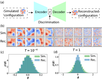
Figure 1: Learning scalar field configuration with autoencoder. (a) schematics of the autoencoder. (b) reconstructed scalar field configuration at different temperatures. (c)-(d) the distribution of simulated vs reconstructed scalar field configurations at (c) $T=10^{-4}$ and (d) $T=1$.

II.3 Autoencoder

The autoencoder is an artificial neural network that is trained to reconstruct its input data in order to learn a compressed representation of the data [14, 2, 49]. It offers a more flexible and computationally efficient approach to dimensionality reduction. We treat the scalar field configurations as pixel intensities and task the autoencoder with reconstructing the configuration of our $\phi^{4}$ scalar field (see schematics in Fig.1 (a)). We use convolutional layers in the autoencoder (see Appendix A.2.1), which promise better reconstruction quality compared to fully-connected layers.

Before attempting to answer the classification question in Sec.II.2, we first show that our autoencoder is capable of capturing the statistics of the scalar field configurations. Fig.1 (b) shows the learning outcomes at different temperatures (5 pairs of random examples at each temperature: top row is simulation, bottom row is reconstruction from autoencoder). The temperature on the right five subfigures is high ($T=1$), and the temperature on the left five subfigures is relatively low ($T=10^{-4}$). For $T=10^{-4}$, the reconstruction quality is high, and the reconstructed configurations almost perfectly resemble the simulated ones. However, for $T=1$ there are still noticeable discrepancies from the simulation, and a possible cause for this discrepancy might be due to the fact that convolutional layers tend to introduce more correlation into the configuration than is present in the simulation in this high temperature phase.

In Fig.1 (c)-(d), we show the distribution of all 300 pairs of simulated and reconstructed configurations at $T=10^{-4}$ and $T=1$. We can see that for $T=10^{-4}$, the two distributions match fairly well, while at $T=1$ there are stronger discrepancies, which agree with our observation in Fig.1 (b).

II.3.1 t-SNE embedding

The latent space in the convolutional autoencoder captures the most salient features of the data in low dimensions. In the convolutional autoencoder described above, although the latent space has only two neurons, the convolutional layers still make the latent space $2\times 7\times 7=98$ dimensional and therefore difficult to interpret by humans. In the following, we use t-SNE embedding [50] to perform dimensionality reduction of the latent space into 2-dimensional (see Appendix A.3.2). Each input configuration becomes a single point in the two-dimensional t-SNE embedded latent space. The data from high-temperature configurations $\mathcal{D}_{h}$ and low-temperature configurations $\mathcal{D}_{l}$ are observed as two distinct groups of points in the embedded space. The goal is to classify these points based on their latent space positions. To achieve this, we can train a binary classifier using the logistic regression algorithm [51] (see Appendix A.3). After the completion of training, the classifier is capable of discerning whether a pair of novel configurations belong to identical or distinct temperatures through examining their positions in the latent space. In the following, we detail this approach which allows for efficient and effective binary classification based on the latent representations of the input configurations.

II.4 Novelty detection: is the temperature same or different?

Logistic regression is a binary classification algorithm that uses a linear decision surface to distinguish two classes of input patterns. Specifically, we treat the latent space points $\boldsymbol{z}^{\mu}$ ($\mu=1,...,300$) as the input for binary classification (see Appendix.A.3). Given data in $\mathcal{D}_{h}$ and $\mathcal{D}_{l}$, we assign the latent representations for samples in $\mathcal{D}_{h}$ with the label $y^{\mu}=+1$ (after passing $\boldsymbol{x}^{\mu}$ from $D_{h}$ through the autoencoder, we obtain $z^{\mu}$ in the latent space and assign $y^{\mu}=1$), and for $\mathcal{D}_{l}$ with the label $y^{\mu}=-1$. For these two classes of $z^{\mu}$, we perform logistic regression to classify them as shown in (Fig.2), and determine the number of correctly classified points. Based on the percentage of correct classification, we can assign a score (see Fig.2).

II.4.1 Comparison with statistical methods

Is the AI method really necessary? We compare our AI method with directly using traditional statistical methods like Principal Component Analysis (PCA) [52] and t-SNE on the raw data, and show that the AI method indeed outperforms such traditional methods. After dimensionality reduction by PCA or t-SNE on the raw data, we perform binary classification as above. Based on the percentage of correct classifications, we can assign scores to PCA (red line in Fig.2(a)) and t-SNE (purple line in Fig.2(a)).

II.4.2 Novelty detection with correlation function value

Additionally, for every scalar field configuration in $D_{h}$ and $D_{l}$, we can measure its $C_{d}/C_{0}$ value (Eq.2, we focus on $d=4$). Now we have two different groups of $C_{d}/C_{0}$ values which form two different histograms in the distribution of $C_{d}/C_{0}$ (Fig.2(d)). Then we can perform binary classification on these values and classify which $C_{d}/C_{0}$ values belong to which dataset ($D_{h}$ or $D_{l}$). The score of $C_{d}/C_{0}$ is shown in the green line in Fig.2(a). Additionally, we report the Receiver-Operator-Characteristic (ROC) curve (see Appendix A.3.3) for the novelty detection result of the convolutional autoencoder and the correlation function (Fig.2(b)).

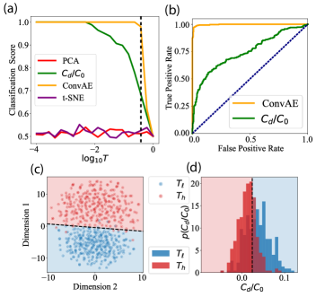
Figure 2: Differentiating temperatures of scalar field sample using different methods. (a) The accuracy score of t-SNE, convolutional autoencoder, PCA, and correlation function as a function of $\mathcal{D}_{l}$’s temperature $T_{l}$. (b)-(d): Example ROC curve (b), t-SNE embedding of the autoencoder latent space (c), and distribution of $C_{d}/C_{0}$ at $T_{l}=0.40$ (corresponds to the dashed line in (a)) (b) The ROC curve of fully-connected autoencoder (yellow line) and $C_{d}/C_{0}$ (green line), dashed line shows the result of a random classifier. (c) The t-SNE embedding of the autoencoder latent space in Section II.3.1. There are two cluster of points with temperature $T_{h}=1$ (red points) and $T_{l}=0.40$ (blue points), and we can see that the points from different datas have little overlap among the decision surface, indicating a good classification result. (d) The distribution of $C_{d}/C_{0}$ values. Red histograms ($T=1$) corresponds to measurements of data from $D_{h}$ and blue histograms ($T=0.40$) corresponds to measurements of datas from $D_{l}$. There is significant overlap between this two clusters, representing a not ideal classification result.

Fig.2(a) shows three curves representing accuracy scores, which indicate the percentage of correct classifications for distinguishing data from $\mathcal{D}_{h}$ or $\mathcal{D}_{l}$ of scalar field configurations. These classifications are obtained using the autoencoder method (the AI method), the principle component analysis method (the statistical method), and the two-point correlation function method (the physics method) under different $T_{l}$ values. In this case, the high-temperature sample ($\mathcal{D}_{h}$) is always set at a temperature of $T_{h}=10^{0}$. We take 20 uniformly distributed points in log space from $[10^{-4},10^{0}]$ and set each of them as the $T_{l}$ for comparison.

The scores $1$ and $0.5$ are two special reference points. A score of $1$ means that our classification is $100\%$ correct, while a score of $0.5$ means that we are guessing blindly and the correctness is equivalent to chance ($50\%$ for binary classification). For the green and yellow lines, there is a relatively stable score within a certain temperature range, followed by a sharp decrease to score $0.5$ as the temperature approaches a certain point for both methods. However, the reduction occurs earlier for the two-point correlation method (around $T=10^{-2}$) compared to the convolutional autoencoder method (around $T=10^{-1.8}$). Additionally, the green line decreases sharply within the temperature range of $[10^{-2},10^{0}]$, and the yellow line falls similarly only when $T\apprge 10^{-0.4}=0.6$. Generally, there is a trend of declining correctness as the temperature increases. Both the PCA method and t-SNE method shows a relatively uniform fluctuation in the score, centered around $0.5$ and oscillating within a range of no more than $0.15$. This is much lower compared to the scores of the convolutional autoencoder method and the two-point correlation function method. We only utilize the first and second principal components for the PCA and t-SNE classification for visualization purposes. However, as shown in the figure, the score is only $0.5$, indicating that two dimensions are not sufficient for these methods.

To show the effectiveness of the convolutional autoencoder, we fix $T_{l}=10^{-0.4}$ to make comparison of the methods’ performance, as shown in Fig.2(b)-(d). In Fig.2(b), there is a ROC curve (see Appendix A.3.3) evaluating the performances of two-point correlation function method and convolutional autoencoder under the temperature such that $T_{h}=10^{0}$ and $T_{l}=10^{-0.4}$. Here, the diagonal (in dashed line) between the coordinate axises refers to the rate of correct classification when making blinding guess, and the ROC curves of convolutional autoencoder and that of two-point correlation function method are shown in yellow and green, respectively. In the diagram, the Area Under the Curve (AUC, also see Appendix.A.3.3) for the curve of convolutional autoencoder is 0.997, which is significantly higher than the AUC for the curve of two-point correlation function, which is 0.748. This gives strong support to our conclusion that convolutional autoencoder is a much better classifier than correlation function in this context.

In Fig.2(c), the points line above the dashed line of the plot are all data from $D_{h}$ (in red) with $T=1,$ and below are from $D_{l}$ with $T=10^{-0.6}$ (in blue). The dotted line represents logistic regression performed on these two classes of points. As the temperature increases, the red points and blue points in the latent space get closer. If the temperature continues to increase, those points will eventually merge together. This is also why, as the temperature increases, it becomes more difficult for the convolutional autoencoder to correctly classify, and the scores decrease sharply.

In Fig.2(d), the histograms show the distribution of values of the correlation function for samples in $D_{h}$ (in red) with $T=1,$ and $D_{l}$ with $T=10^{-0.6}$ (in blue). There is also a decision surface in between the two histograms to separate the $C_{d}/C_{0}$ values from the $D_{h}$ and $D_{l}$ data. The points to the left of the decision surface belong to $D_{h}$ and the points to the right belong to $D_{l}$. As we can see, there is a significant overlap between the two histograms, and the classification fails in this overlap region, resulting in a lower classification score.

The PCA score shows a relatively uniform fluctuation around 0.5, which is essentially equal to chance, indicating that the first two principal components alone are insufficient for correct classification. Since a linear autoencoder is equivalent to PCA, when comparing the classification performance of the two-dimensional embedded latent space of the (nonlinear) autoencoder, we conclude that nonlinearity is necessary for this task. Thus, we cannot use traditional methods like PCA for this classification task while requiring good visualization of the decision process (2-dimensional). Similarly, performing t-SNE directly on the original data yields poor classification results. This justifies our use of AI methods (autoencoder) over traditional statistical methods (PCA and t-SNE). In conclusion, we find that autoencoder-based classification of different temperatures outperforms both statistics methods (PCA and t-SNE) and physical metrics (correlation function).

III Conclusion and discussion

III.1 Conclusion

In this paper, we study the problem of differentiating between different temperatures in scalar field samples, serving as a toy model for detecting subtle macroscopic changes in a many-body system. We used a convolutional autoencoder (AI method), PCA and t-SNE (statistical methods), and the two-point correlation function (physics method) to distinguish samples of scalar field configurations with increasingly close temperatures. Additionally, we also attempted to compress the high-dimensional configuration of the scalar field and reconstruct it from the low-dimensional latent space of an autoencoder. Based on the results we have collected, we show that the autoencoder is able to capture realistic statistics of the scalar field, similar to physical simulations. We also demonstrate that both the latent space of the autoencoder and the two-point correlation function can be used to perform classification of different temperatures for the scalar field, while the AI method (convolutional autoencoder) outperforms the physical method (two-point correlation) as well as the statistical methods (PCA and t-SNE).

Our study can still be further optimized in a number of ways. The statistics of the high-temperature phase of the scalar field system can potentially be better captured by improving the structure of the autoencoder. Furthermore, while we focus only on a scalar field at equilibrium, we can couple the scalar field to an external source to drive the system out of equilibrium, which would be of interest for more realistic non-equilibrium many-body systems. We can also extend our method to more sophisticated models, such as vector fields (multiple component fields), and use the AI method we presented to differentiate other physical quantities such as magnetization, free energy, and dissipation. Finally, it would also be interesting to explore whether our results can be applied to detect macroscopic changes in experimental many-body systems.

Appendix A Correlation function scaling

A.1 Scalar field simulation

A.1.1 Monte-Carlo simulation

To obtain the massive scalar field system in equilibrium, we utilize the Metropolis-Hastings algorithm. This algorithm employs Monte Carlo methods to update the configuration of these scalars $\phi$ with random samples obtained from the Boltzmann distribution $P$ determined by the Hamiltonian $H$ of the field

$$P(\phi)=e^{-\beta H(\phi)}.$$ (3)

Here, $\beta$ stands for the inverse temperature defined as $1/K_{B}T$, where $K_{B}$ refers to Boltzmann constant, and $T$ refers to temperature of the system.

To start our simulation, we initialize a random configuration of scalars $\phi$ that follows a normal distribution. We then calculate the Hamiltonian of this configuration, denoted as $H[\phi]$ (Eq.1), along with its associated probability $P(\phi)$ (Eq.3). During each Monte-Carlo sweep, we randomly propose a new configuration $\phi^{\prime}$ drawn from normal distribution, and calculate the Hamiltonian of the current configuration $H[\phi^{\prime}]$ and its associated probability $P(\phi^{\prime})$.

If $\triangle H<0$, the new configuration $\phi^{\prime}$ is always accepted and used as the new $\phi$ for the next sweep.

If $\triangle H>0$, by contrast, our acceptance is determined by $r$, the acceptance probability is calculated as

$$r=\frac{P(\phi^{\prime})}{P(\phi)}=e^{\beta(H[\phi^{\prime}]-H[\phi])}\equiv e^{\beta(\triangle H)},$$ (4)

where $\triangle H=H[\phi^{\prime}]-H[\phi]$.

Throughout all the simulations conducted in this paper, we choose $m^{2}=0.1$ and $\lambda=0.01$. For each temperature ($20$ of them) used in the current study, we perform $300$ independent realizations of the scalar field simulation.

A.1.2 Finite size effects

In this section, we study potential finite size effects on the two-point correlation function (Eq.2). We simulate the scalar field in Eq.1 for different lattice sizes and report the measured $C_{d}/C_{0}$ in Fig.3.

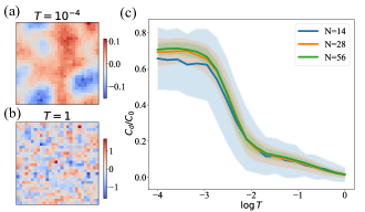
Figure 3: Differentiating sample temperatures among different methods. (a) typical configuration of $\phi$ in a low-temperature($T=10^{-4}$) phase. (b) typical configuration of $\phi$ in a high-temperature ($T=10^{0}$) phase. (c) Average value of two-point correlation function for $\phi$ in different temperatures($T\in[10^{-4},10^{0}]$) for three different sizes of the system($N=14,28,56$), one standard deviation is included as shade.

In Fig.3 (a)-(b), we show the configurations of the highest and lowest temperatures of the scalar field we studied. When comparing Fig.3(a) with Fig.3(b) , it is evident that the phase shown in (a) is more ordered than (b). There are many large areas with similar colors, indicating similar scalar values between neighboring scalars in these areas. This is because at low temperature ($T=10^{-4}$), there are negligible random noises compared to the system at high temperature $(T=10^{0})$, and cooperativity dominates the interactions between scalars. Additionally, a much smaller range of $\phi$ values is observed in the lower temperature phase. In contrast, the pattern in Fig.3 (b) appears to be very chaotic, with the values of most neighboring scalars varying much more, leading to fewer coherent areas.

In Fig.3(c), we show values of the two-point correlation function (Eq.2) for $N=14,28,56$ when the temperature changes in the range of $[10^{-4},10^{0}]$. Solid lines are the mean value and shades correspond to one standard deviation. Initially (at around $T=10^{-4}$), the mean correlation value is higher for larger sizes. However, although the value still increases with increasing size at the same temperature, the difference between the three lines in the vertical section becomes negligible as $T$ increases. Furthermore, the phase-transition temperatures for these three conditions are similar to the others, occurring at approximately $T=10^{-2.5}$. Therefore, we conclude that within the purpose of this study, the effect of different sizes $N$ can be neglected when using $C_{d}/C_{0}$ for differentiating different scalar field temperatures. Thus, we fixed $N=28$ for all other simulations performed in this paper.

A.2 Autoencoder

The autoencoder consists of an encoder $g(\boldsymbol{x}^{\mu})=\boldsymbol{z}^{\mu}$, which compresses the input data $\boldsymbol{x}^{\mu}$ into a latent feature representation $\boldsymbol{z}^{\mu}$, and a decoder $f(\boldsymbol{z}^{\mu})=f(g(\boldsymbol{x}^{\mu})):=\tilde{\boldsymbol{x}}^{\mu}$ that decompresses the latent feature representation into a reconstructed output $\tilde{\boldsymbol{x}}^{\mu}$. The reconstruction quality is commonly assessed using a loss function that measures the disparity between the original input and the reconstructed output. We use the mean-square error (MSE) between the input $\boldsymbol{x}^{\mu}$ and the output $\boldsymbol{\tilde{x}}^{\mu}$ as the loss function for the autoencoder.

Overfitting arises when a model excessively fits the training data, leading to worse performance on unseen data. To avoid overfitting, we introduce an additional $L_{2}$ regularization into the loss function, which discourages the model from acquiring overly intricate patterns within the training data and encourages sparsity of the latent feature output:

$$L=\frac{1}{P}\overset{P}{\underset{\mu=1}{\sum}}||\boldsymbol{x}^{\mu}-\tilde{\boldsymbol{x}}^{\mu}||^{2}+\gamma\underset{i}{\sum^{M}}||\boldsymbol{\theta}_{i}^{2}||,$$ (5)

where $P$ represents the number of data in the dataset ($P=300$), $\boldsymbol{x}^{\mu}$ and $\tilde{\boldsymbol{x}}^{\mu}$ represent the original input and reconstructed output for the $\mu^{th}$ observation, $\boldsymbol{\theta}_{i}$ represents the $i^{th}$ parameters (weights and biases) in the functions $f$ and $g$. Using the sum of the squared difference between the original input and the reconstructed output for the $\mu^{th}$ observation means that the reconstructed outputs are encouraged to be close to the original inputs. For regularization terms added to mitigate the overfitting problem, $\gamma$ is a regularization parameter that controls the trade-off between the reconstruction error and the penalty term. As $\gamma$ approaches zero, the weight of the $L_{2}$ regularization term becomes very small and has almost no penalizing effect on the parameters. This makes the model focus more on reducing the loss function itself and less on the sparsity of the parameters. When $\gamma$ tends to infinity, the weight of the $L_{2}$ regularization item becomes very large, which leads to a stronger tendency to choose a sparse feature model. $\gamma$ can be arbitrary, and it is usually a small number (as regularization and reconstruction compete with each other, we typically pick $\gamma=10^{-6}$ to ensure good reconstruction quality).

A.2.1 Convolutional Autoencoder

In the following, we outline the architecture of the autoencoder used for such reconstruction tasks. Fig.1(a) illustrates the general structure of an autoencoder, which consists of two main parts: the encoder and the decoder.

Encoder: The encoder starts with an input layer, which expects images of shape $28\times 28\times 1$. It then applies a series of layers to this input: (1) a convolutional layer with 32 filters, each of size $3\times 3$ (with linear activation); (2) a max pooling layer with a pool size of $2\times 2$; (3) a convolutional layer with 32 filters, each of size $3\times 3$ (with ReLU activation); (4) a max pooling layer with a pool size of $2\times 2$; (5) a dense layer with 2 units (with ReLU activation). This layer represents the bottleneck layer, which is the encoded version of the input.

Decoder: The decoder takes the output of the encoder and applies a series of layers to reconstruct the original input: (1) a transposed convolutional (deconvolutional) layer with 32 filters, each of size $3\times 3$ and a stride of 2 (with ReLU activation); (2) a transposed convolutional layer with 32 filters, each of size $3\times 3$ and a stride of 2 (with ReLU activation); (3) a convolutional layer with 1 filter of size $3\times 3$ (with linear activation). This layer reconstructs the original input from the encoded representation.

We use the same padding throughout all the convolutional layers.

A.3 Binary classification

For a given input sample $\boldsymbol{x}^{\mu}$, we use the sigmoid function $\sigma$ as our classifier, and the predicted output $\hat{y}^{\mu}$ is calculated as follows:

$$\hat{y}^{\mu}=\sigma(\boldsymbol{w}^{T}\boldsymbol{x}^{\mu})=\frac{1}{1-e^{-\boldsymbol{w}^{T}\boldsymbol{x}^{\mu}}}.$$ (6)

To generate the maximum-margin solution within our capacity, we use cross-entropy as our loss function under the condition where the weight will be the most robust and generalizable to other similar inputs

$$\mathcal{L}=\frac{1}{P}\underset{\mu}{\sum}\left[y^{\mu}\ln\hat{y}^{\mu}+(1-y^{\mu})\ln(1-\hat{y}^{\mu})\right],$$ (7)

where $P$ refers to the number of data samples $\boldsymbol{x}^{\mu}$, and $\mu$ indexes the data. $y^{\mu}$ and $\hat{y}^{\mu}$ refer to the actual and predicted outputs for the $\mathord{\mu}^{th}$ input data $\boldsymbol{x}^{\mu}$, respectively.

We use gradient descent $\frac{\partial\mathcal{L}}{\partial\overrightarrow{w}}$ based on the loss function $\mathcal{L}$ to update the weight, which is given by

$$\frac{\partial\mathcal{L}}{\partial\overrightarrow{w}}=\frac{1}{p}\underset{\mu}{\sum}\left(\hat{y}^{\mu}-y^{\mu}\right)\boldsymbol{x}^{\mu}.$$ (8)

Our classification result is a binary distribution as a function of $\hat{y}^{\mu}$. Given data $\boldsymbol{x}^{\mu}$, the probability of the true label $y^{\mu}$ being equal to 1 is $\hat{y}^{\mu}$

$$P(y^{\mu}=1\mid\boldsymbol{x}^{\mu})=\hat{y}^{\mu},$$ (9)

and given data $\boldsymbol{x}^{\mu}$, the probability of true label $y^{\mu}$ equals to $-1$ is $1-\hat{y}^{\mu}$

$$P(y^{\mu}=-1\mid\boldsymbol{x}^{\mu})=1-\hat{y}^{\mu}.$$ (10)

A.3.1 Principal Component Analysis (PCA)

PCA is used to analyze large datasets with high dimensions, improving data interpretability while retaining the maximum amount of information and enabling multidimensional data display. It aims to find a projection of the data onto directions that maximize the variance of the original dataset. The PCA algorithm can reduce the dimensionality of data to provide a clearer understanding and visualization. Additionally, the PCA algorithm is fast and does not require parameter tuning or optimization. However, its disadvantage is that it is based solely on covariance ($2^{nd}$ order statistics) and is limited to linear projections. PCA can also be used to denoise and compress data, as well as identify informative variables that better explain the data.

Given a dataset $\left\{\boldsymbol{x}^{\mu}\right\}_{\mu=1}^{P}$, we subtract the mean $\left\langle\boldsymbol{x}\right\rangle$ from the data, resulting in $\left\{\boldsymbol{x}^{\mu}-\left\langle\boldsymbol{x}\right\rangle\right\}_{\mu=1}^{P}.$ Then, we find the principal components $\boldsymbol{e}_{i},i=1,...,N$ of the dataset. We then project the data onto the first $M$ principal directions ($M=2$ in the main text) and add back the mean to obtain the reconstructed data,

$$\tilde{\boldsymbol{x}}^{\mu}=\sum_{i=1}^{M}\left(\boldsymbol{x}^{\mu}-\left\langle\boldsymbol{x}\right\rangle\right)^{T}\boldsymbol{e}_{i}+\left\langle\boldsymbol{x}\right\rangle$$ (11)

A.3.2 t-distributed Stochastic Neighbor Embedding (t-SNE)

t-SNE is a statistical method , an embedding model (data is usually embedded in two or three dimensions) for reducing high-dimensional data and visualizing data. Basically, it transfers the distance of high-dimensional data points to probability distribution and models a similar low-dimensional data using these distances.

Assume we have a $N$ dimension data $\boldsymbol{x}_{1-N}$. Firstly, the t-SNE algorithm constructs a probability distribution over high-dimensional object pairs so that points that are dissimilar are allocated a lower probability, while objects that are similar are assigned a greater probability. Then, we generate the same amount of low-dimensional data at random $y_{1-N}$.

For each high-dimensional data point $x_{i}$, we define a conditional probability distribution $p_{j\mid i}$, where $i\neq j$

$$p_{j\mid i}=\frac{\exp(-\parallel x_{i}-x_{j}\parallel^{2}/2\sigma_{i}^{2})}{\sum_{k\neq i}\exp(-\parallel x_{i}-x_{k}\parallel^{2}/2\sigma_{i}^{2})},$$ (12)

and set $p_{i\mid i}=0$. Note that $\underset{j}{\sum}p_{j\mid i}=1$ for all $i$. Then we define the similarity of high-dimensional data as $p_{ij}$

$$p_{ij}=\frac{p_{j\mid i}+p_{i\mid j}}{2N}.$$ (13)

For low-dimensional data $y_{1-N}$, we similarity define a $q_{ij}$

$$q_{ij}=\frac{(1+\parallel y_{j}-y_{i}\parallel^{2})^{-1}}{\sum_{k}\sum_{l\neq k}(1+\parallel y_{k}-y_{l}\parallel^{2})^{-1}}.$$ (14)

We would like to measure the difference between two probability distributions (high-dimensional distribution $p_{ij}$ and low-dimensional distribution $q_{ij}$), with respect to the location of data points. Here we use Kullback–Leibler divergence (KL divergence) to calculate the difference. We use KL divergence as the lost function $L$,

$$L=KL(p\parallel q)=\sum_{i,j}p_{i,j}\log\frac{p_{i,j}}{q_{i,j}}.$$ (15)

Finally, we use gradient descent to minimize the KL divergence and update low-dimensional data to make it as similar as the high-dimensional data as possible until the algorithm converges.

After these steps, the t-SNE algorithm maps data from a high-dimensional space to a low-dimensional space, which forms clusters in low-dimensional data and preserves a local atlas of high-dimensional data.

A.3.3 Receiver Operating Characteristic (ROC) curve

The ROC (Receiver Operating Characteristic) curve is a graphical representation that showcases the diagnostic ability of a binary classifier system. It is created by plotting the TPR (true positive rate) against the FPR (false positive rate) at various classification thresholds. For models with fixed thresholds, data that has been classified can result in four different scenarios, namely $TP$ (True Positive), $TN$ (True Negative), $FP$ (False Positive,Type I error), and $FN$ (False Negative,Type II error).

The $TPR$ is the ratio of correctly classified positive instances to all positive instances ($P$), which means the number of real positive cases in the data:

$$TPR=\frac{TP}{P}=\frac{TP}{TP+FN}.$$ (16)

The $FPR$ is the ratio of incorrectly classified negative instances to all negative instances, which means the number of real negative cases in the data:

$$FPR=\frac{FP}{N}=\frac{FP}{FP+TN}.$$ (17)

The ROC curve provides a comprehensive picture of the classifier’s performance by illustrating the trade-off between the true positive rate and the false positive rate. In an ideal scenario, the TPR is 1 and the FPR is 0, implying a perfect classifier that makes no false predictions. This ideal situation is represented by a point on the top-left corner of the ROC curve.

The area under the ROC curve (AUC) is used as a measure of the classifier’s performance. The AUC ranges from 0 to 1, with a higher value indicating better discrimination ability. An AUC of 0.5 signifies that the classifier performs no better than random guessing, while an AUC of 1 represents a perfect classifier. On the contrary, when the value is 0, the result is exactly the opposite of the answer.

The ROC curve provide a simple and intuitive way to compare and select the best model among multiple candidates. A model with a higher AUC is generally preferred as it demonstrates better predictive accuracy. Moreover, it offer a visual representation of the classifier’s quality and help choose an optimal classification threshold based on the desired trade-off between the true positive rate and the false positive rate.

References

- [1] Yann LeCun, Yoshua Bengio, and Geoffrey Hinton. Deep learning. nature, 521(7553):436–444, 2015.
- [2] Ian Goodfellow, Yoshua Bengio, and Aaron Courville. Deep learning. MIT press, 2016.
- [3] David Silver, Aja Huang, Chris J Maddison, Arthur Guez, Laurent Sifre, George Van Den Driessche, Julian Schrittwieser, Ioannis Antonoglou, Veda Panneershelvam, Marc Lanctot, et al. Mastering the game of go with deep neural networks and tree search. nature, 529(7587):484–489, 2016.
- [4] David Silver, Julian Schrittwieser, Karen Simonyan, Ioannis Antonoglou, Aja Huang, Arthur Guez, Thomas Hubert, Lucas Baker, Matthew Lai, Adrian Bolton, et al. Mastering the game of go without human knowledge. nature, 550(7676):354–359, 2017.
- [5] Jascha Sohl-Dickstein, Eric Weiss, Niru Maheswaranathan, and Surya Ganguli. Deep unsupervised learning using nonequilibrium thermodynamics. In International conference on machine learning, pages 2256–2265. PMLR, 2015.
- [6] Jonathan Ho, Ajay Jain, and Pieter Abbeel. Denoising diffusion probabilistic models. Advances in neural information processing systems, 33:6840–6851, 2020.
- [7] Robin Rombach, Andreas Blattmann, Dominik Lorenz, Patrick Esser, and Björn Ommer. High-resolution image synthesis with latent diffusion models. In Proceedings of the IEEE/CVF conference on computer vision and pattern recognition, pages 10684–10695, 2022.
- [8] Ashish Vaswani, Noam Shazeer, Niki Parmar, Jakob Uszkoreit, Llion Jones, Aidan N Gomez, Łukasz Kaiser, and Illia Polosukhin. Attention is all you need. Advances in neural information processing systems, 30, 2017.
- [9] Sébastien Bubeck, Varun Chandrasekaran, Ronen Eldan, Johannes Gehrke, Eric Horvitz, Ece Kamar, Peter Lee, Yin Tat Lee, Yuanzhi Li, Scott Lundberg, et al. Sparks of artificial general intelligence: Early experiments with gpt-4. arXiv preprint arXiv:2303.12712, 2023.
- [10] Giuseppe Carleo, Ignacio Cirac, Kyle Cranmer, Laurent Daudet, Maria Schuld, Naftali Tishby, Leslie Vogt-Maranto, and Lenka Zdeborová. Machine learning and the physical sciences. Reviews of Modern Physics, 91(4):045002, 2019.
- [11] John Jumper, Richard Evans, Alexander Pritzel, Tim Green, Michael Figurnov, Olaf Ronneberger, Kathryn Tunyasuvunakool, Russ Bates, Augustin Žídek, Anna Potapenko, et al. Highly accurate protein structure prediction with alphafold. Nature, 596(7873):583–589, 2021.
- [12] Hanchen Wang, Tianfan Fu, Yuanqi Du, Wenhao Gao, Kexin Huang, Ziming Liu, Payal Chandak, Shengchao Liu, Peter Van Katwyk, Andreea Deac, et al. Scientific discovery in the age of artificial intelligence. Nature, 620(7972):47–60, 2023.
- [13] John J Hopfield. Neural networks and physical systems with emergent collective computational abilities. Proceedings of the national academy of sciences, 79(8):2554–2558, 1982.
- [14] Geoffrey E Hinton and Ruslan R Salakhutdinov. Reducing the dimensionality of data with neural networks. science, 313(5786):504–507, 2006.
- [15] Daniel J Amit, Hanoch Gutfreund, and Haim Sompolinsky. Storing infinite numbers of patterns in a spin-glass model of neural networks. Physical Review Letters, 55(14):1530, 1985.
- [16] Hyunjune Sebastian Seung, Haim Sompolinsky, and Naftali Tishby. Statistical mechanics of learning from examples. Physical review A, 45(8):6056, 1992.
- [17] Andreas Engel. Statistical mechanics of learning. Cambridge University Press, 2001.
- [18] Elizabeth Gardner. The space of interactions in neural network models. Journal of physics A: Mathematical and general, 21(1):257, 1988.
- [19] Yasaman Bahri, Jonathan Kadmon, Jeffrey Pennington, Sam S Schoenholz, Jascha Sohl-Dickstein, and Surya Ganguli. Statistical mechanics of deep learning. Annual Review of Condensed Matter Physics, 11:501–528, 2020.
- [20] Juan Carrasquilla and Roger G Melko. Machine learning phases of matter. Nature Physics, 13(5):431–434, 2017.
- [21] Akinori Tanaka and Akio Tomiya. Detection of phase transition via convolutional neural networks. Journal of the Physical Society of Japan, 86(6):063001, 2017.
- [22] Evert PL Van Nieuwenburg, Ye-Hua Liu, and Sebastian D Huber. Learning phase transitions by confusion. Nature Physics, 13(5):435–439, 2017.
- [23] Dmitrii Kochkov, Jamie A Smith, Ayya Alieva, Qing Wang, Michael P Brenner, and Stephan Hoyer. Machine learning–accelerated computational fluid dynamics. Proceedings of the National Academy of Sciences, 118(21):e2101784118, 2021.
- [24] Frank Noé, Alexandre Tkatchenko, Klaus-Robert Müller, and Cecilia Clementi. Machine learning for molecular simulation. Annual review of physical chemistry, 71:361–390, 2020.
- [25] Giuseppe Carleo and Matthias Troyer. Solving the quantum many-body problem with artificial neural networks. Science, 355(6325):602–606, 2017.
- [26] Weishun Zhong, Jacob M Gold, Sarah Marzen, Jeremy L England, and Nicole Yunger Halpern. Machine learning outperforms thermodynamics in measuring how well a many-body system learns a drive. Scientific Reports, 11(1):9333, 2021.
- [27] Hsin-Yuan Huang, Richard Kueng, Giacomo Torlai, Victor V Albert, and John Preskill. Provably efficient machine learning for quantum many-body problems. Science, 377(6613):eabk3333, 2022.
- [28] Keith T Butler, Daniel W Davies, Hugh Cartwright, Olexandr Isayev, and Aron Walsh. Machine learning for molecular and materials science. Nature, 559(7715):547–555, 2018.
- [29] Weishun Zhong, Jacob M Gold, Sarah Marzen, Jeremy L England, and Nicole Yunger Halpern. Quantifying many-body learning far from equilibrium with representation learning. arXiv preprint arXiv:2001.03623, 2020.
- [30] Weishun Zhong. Non-equilibrium physics: from spin glasses to machine and neural learning. arXiv preprint arXiv:2308.01538, 2023.
- [31] Zackery A Benson, Anton Peshkov, Nicole Yunger Halpern, Derek C Richardson, and Wolfgang Losert. Experimentally measuring rolling and sliding in three-dimensional dense granular packings. Physical Review Letters, 129(4):048001, 2022.
- [32] Sayantan Majumdar, Louis C Foucard, Alex J Levine, and Margaret L Gardel. Mechanical hysteresis in actin networks. Soft matter, 14(11):2052–2058, 2018.
- [33] Joseph D Paulsen, Nathan C Keim, and Sidney R Nagel. Multiple transient memories in experiments on sheared non-brownian suspensions. Physical review letters, 113(6):068301, 2014.
- [34] Zijun Li and Jiming Yang. Dynamical phase transition in random walk subject to random drives. arXiv preprint arXiv:2209.08605, 2022.
- [35] Srimayee Mukherji, Neelima Kandula, AK Sood, and Rajesh Ganapathy. Strength of mechanical memories is maximal at the yield point of a soft glass. Physical review letters, 122(15):158001, 2019.
- [36] Jordan Hoffmann, Yohai Bar-Sinai, Lisa M Lee, Jovana Andrejevic, Shruti Mishra, Shmuel M Rubinstein, and Chris H Rycroft. Machine learning in a data-limited regime: Augmenting experiments with synthetic data uncovers order in crumpled sheets. Science advances, 5(4):eaau6792, 2019.
- [37] Weishun Zhong, David J Schwab, and Arvind Murugan. Associative pattern recognition through macro-molecular self-assembly. Journal of Statistical Physics, 167:806–826, 2017.
- [38] Constantine Glen Evans, Jackson O’Brien, Erik Winfree, and Arvind Murugan. Pattern recognition in the nucleation kinetics of non-equilibrium self-assembly. arXiv preprint arXiv:2207.06399, 2022.
- [39] Jirawat Tangpanitanon, Supanut Thanasilp, Ninnat Dangniam, Marc-Antoine Lemonde, and Dimitris G Angelakis. Expressibility and trainability of parametrized analog quantum systems for machine learning applications. Physical Review Research, 2(4):043364, 2020.
- [40] Weishun Zhong, Xun Gao, Susanne F Yelin, and Khadijeh Najafi. Many-body localized hidden born machine. arXiv preprint arXiv:2207.02346, 2022.
- [41] Maksym Serbyn, Dmitry A Abanin, and Zlatko Papić. Quantum many-body scars and weak breaking of ergodicity. Nature Physics, 17(6):675–685, 2021.
- [42] James P Sethna. Statistical mechanics: entropy, order parameters, and complexity, volume 14. Oxford University Press, USA, 2021.
- [43] Kai Zhou, Gergely Endrődi, Long-Gang Pang, and Horst Stöcker. Regressive and generative neural networks for scalar field theory. Physical Review D, 100(1):011501, 2019.
- [44] Javad Komijani and Marina K Marinkovic. Generative models for scalar field theories: how to deal with poor scaling? arXiv preprint arXiv:2301.01504, 2023.
- [45] Jan M Pawlowski and Julian M Urban. Reducing autocorrelation times in lattice simulations with generative adversarial networks. Machine Learning: Science and Technology, 1(4):045011, 2020.
- [46] Luigi Del Debbio, Joe Marsh Rossney, and Michael Wilson. Efficient modeling of trivializing maps for lattice 4 theory using normalizing flows: a first look at scalability. Physical Review D, 104(9):094507, 2021.
- [47] Mark Srednicki. Quantum field theory. Cambridge University Press, 2007.
- [48] Mehran Kardar. Statistical physics of fields. Cambridge University Press, 2007.
- [49] Dor Bank, Noam Koenigstein, and Raja Giryes. Autoencoders. Machine Learning for Data Science Handbook: Data Mining and Knowledge Discovery Handbook, pages 353–374, 2023.
- [50] Geoffrey E Hinton and Sam Roweis. Stochastic neighbor embedding. Advances in neural information processing systems, 15, 2002.
- [51] Scott Menard. Applied logistic regression analysis. Number 106. Sage, 2002.
- [52] Jonathon Shlens. A tutorial on principal component analysis. arXiv preprint arXiv:1404.1100, 2014.