Model Predictive Control for Aggressive Driving Over Uneven Terrain

Abstract

Terrain traversability in off-road autonomy has traditionally relied on semantic classification or resource-intensive dynamics models to capture vehicle-terrain interactions. However, our experiences in the development of a high-speed off-road platform have revealed several critical challenges that are not adequately addressed by current methods at our operating speeds of 7–10 m/s. This study focuses particularly on uneven terrain geometries such as hills, banks, and ditches. These common high-risk geometries are capable of disabling the vehicle and causing severe passenger injuries if poorly traversed. We introduce a physics-based framework for identifying traversability constraints on terrain dynamics. Using this framework, we then derive two fundamental constraints, with a primary focus on mitigating rollover and ditch-crossing failures. In addition, we present the design of our planning and control system, which uses Model Predictive Control (MPC) and a low-level controller to enable the fast and efficient computation of these constraints to meet the demands of our aggressive driving. Through real-world experimentation and traversal of hills and ditches, our approach is tested and benchmarked against a human expert. These results demonstrate that our approach captures fundamental elements of safe and aggressive control on these terrain features.

I Introduction

Autonomous vehicles have the potential to be applied to agriculture, transportation in underdeveloped cities, and search and rescue [1, 2, 3]. To succeed in these applications, autonomous vehicles must be able to operate without a priori knowledge in unstructured and off-road environments, which violate assumptions commonly made in on-road autonomous vehicle research [4, 5]. In particular, unlike the on-road setting, successful off-road driving depends critically on safe traversal of uneven terrain such as hills, ditches, banks, and bumps. We aim to address two significant failure risks with traversing such terrain. First, a failure by rollover occurs when the vehicle becomes disabled by tipping onto its sides. The risk of rollovers is substantially higher in off-road driving where steep hills, sharp turns, and high centers of mass are common. The second failure risk is associated with ditches. Often characterized by sudden and disruptive depressions in elevation, ditches are ill-defined where mentioned in the literature and can greatly depend on the system and the environment [6, 7]. Failures due to ditches involve, for example, launching into the air and crashing into the ground (fig. 1.2). Either rollovers or ditches are easily capable of disabling the vehicle and causing severe bodily harm. In our work, we aim to enable safe, agile, and efficient planning and control for unstructured off-road environments with these uneven terrain geometries.

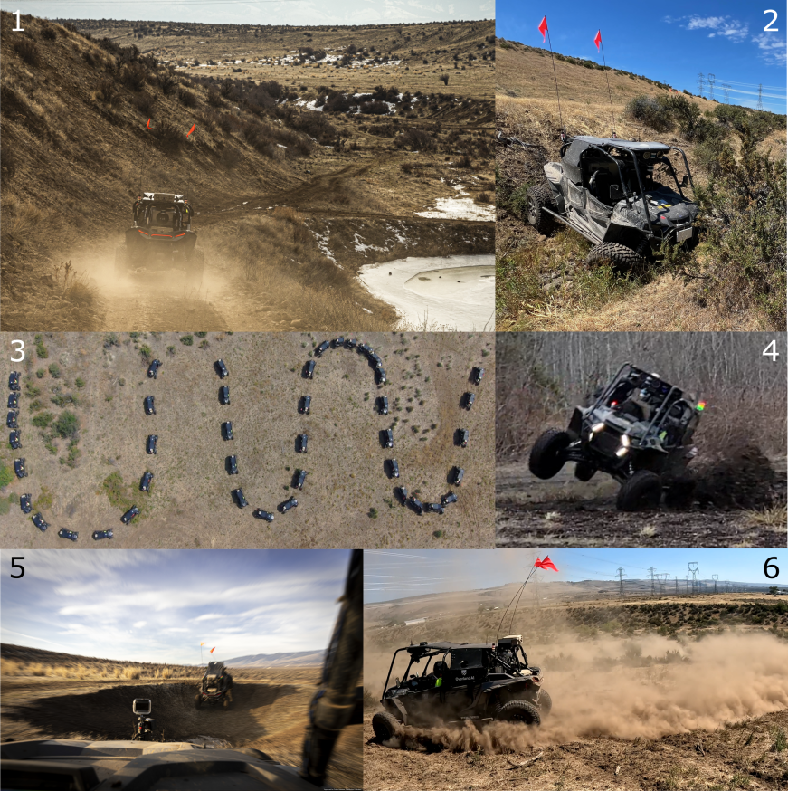
Figure 1: (1) Robot in uneven terrain. (2) Poor ditch traversal. (3) Action sequence of bird’s-eye-view of “UW” slalom on hill. (4) Poor rollover handling. (5) Chasing robot through crater ditch. (6) Expert driver performing aggressive circles. Note that (2) and (4) are not outcomes of our approach.

Existing work on autonomous navigation of uneven terrain generally estimate roll and pitch angles by using only the geometry of the terrain [8, 9, 10]. Although this may be sufficient at lower speeds, this approach becomes increasingly inaccurate and unsafe at higher speeds due to dynamic effects, from unmodeled forces and vehicle inertia. These effects have been extensively investigated in research related to automobile safety testing for analyzing rollovers. This work primarily proposes metrics such as static stability factor [11, 12], lateral load transfer ratio [13, 14, 15, 16, 17], time to rollover [18, 19], etc. Unfortunately, these metrics do not provide deep insight into maneuver failure due to ditches. A very different approach to ditch traversal has been proposed using imitation learning [20]. However, it does not take into account dynamic effects, which are critical for safe ditch traversal, similar to rollovers. Furthermore, due to the diversity of terrain geometry in natural environments, we cannot simply categorize ditches as a special handling class with a distinct control policy. We propose contending with potential rollovers and ditches by estimating the implicit forces of sampled paths, similar to [21]. We further generalize this approach for ditches, without assuming a nominally flat path and within the context of real-time control.

We deploy our methods on real-world platforms, overcoming additional system-level challenges for aggressive off-road navigation. At an operating speed of $7$–$10$ m/s, our control system needs to meet a target frequency of $30$ Hz or higher to ensure safe and reliable operation, making fast planning and re-planning extremely important. Low control rates would cause the system to encounter issues with misrepresented or delayed semantic obstacles and terrain geometries. This high control rate also makes using accurate but complex 3D models impractical. For example, while [22] implements a 3D rigid-body model considering tire forces, the resulting nonlinear MPC implementation operates at less than 3 Hz, about one tenth of our target control rate. In [23], the proposed approach is validated only in simulation at a much lower operating speed of 3 m/s and over gentler ground geometries. Learning-based dynamics modeling has also been proposed in the literature [24, 25, 26]. However, learning accurate dynamics for aggressive driving requires substantial amount of data near the safety limits of the vehicle. This can be dangerous and may not be feasible in practice.

We present two main contributions to off-road autonomy in this paper. First, we propose a physics-based framework to analyze traversability constraints for a mobile robot on uneven terrain. Similar to methods designed to prevent rollovers, we present a quantification metric useful for traversing ditches. To the best of our knowledge, this is the first approach in the literature to ditch traversal for autonomous off-road driving at higher operating speeds. Second, we propose a full planning and control solution to off-road navigation validated on a full-scale Polaris RZR UTV equipped with onboard sensing and compute. The planning and control system consists of a planner based on the model predictive path integral (MPPI) algorithm [27, 28], and a low-level feedforward-feedback controller. Within the MPPI framework, we evaluate kinematically sampled trajectories with our traversability constraints implemented as costs. Doing so avoids the computational complexity of a full dynamical model while still achieving safe operation. We also present the system design, heuristics, and results from real-world iterative testing. Our results are benchmarked against an expert driver to better evaluate the aggressiveness of our autonomy.

II Preliminaries

II-A Sample-Based Model Predictive Control

We employ sample-based Model Predictive Control (MPC)  [29, 27, 28]. Let $\mathbf{x}_{t}$ and $\mathbf{u}_{t}$ represent state and control at time $t$. For a given control horizon $H$, we randomly sample $N$ open-loop control sequences $\{\mathbf{u}_{t:t+H-1}^{i}\}_{i=1}^{N}$. For each sequence, we compute their cumulative costs over the horizon $C(\mathbf{u}_{t:t+H-1}^{i};\mathbf{x}_{t})\coloneqq\sum^{H-1}_{h=0}c(\mathbf{x}_{t+h},\mathbf{u}_{t+h})$ using the predicted trajectory rollout given by the bicycle kinematics model [30]. Without a priori knowledge of the environment, a model of the terrain dynamics can be impractical or altogether inaccessible. As inaccurate global models are known to result in poor performance for MPC [28], the abstracted bicycle model leverages the lower-level controller to better handle unmodeled terrain dynamics. With this model, our state can be represented by $\mathbf{x}_{t}=\begin{pmatrix}x_{t}&y_{t}&\psi_{t}\end{pmatrix}$ where $\begin{pmatrix}x_{t}&y_{t}\end{pmatrix}$ is the position of the center of mass and $\psi_{t}$ is the heading. Our control is then represented by $\mathbf{u}_{t}=\begin{pmatrix}v_{t}&\kappa_{t}\end{pmatrix}$ where $v_{t}$ is the linear velocity and $\kappa_{t}$ is the steering curvature. To obtain the optimal control command for the vehicle, we use the update law given by the model-predictive path integral (MPPI) control algorithm [31, 28]. This family of MPC algorithms have become increasingly popular due to their flexibility with non-differentiable cost functions and parallelizability, especially with a kinematic model [29, 28].

II-B Attitude Angles Using Elevation Map

The elevation map provides MPPI with the perceived height of the ground at the map’s physical location. This is a common representation for ground geometry where sensor input is provided by LiDAR or stereo cameras [32, 33, 34, 35]. As done in [22, 24, 23], we use these elevations to estimate the vehicle’s attitude angles (roll $\phi$ and pitch $\theta$) assuming the vehicle wheels are rigidly attached to the elevation map and are co-planar, as demonstrated in fig. 2.

III Physics-Based Traversability Constraints

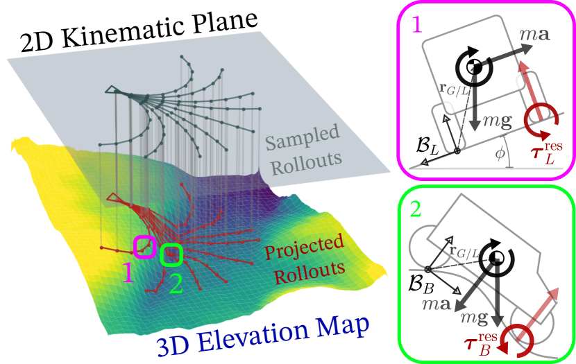
Figure 2: Rollouts are sampled in the 2D kinematic plane then constrained by their implicit dynamics on the elevation map (left). Frames and forces for rollover analysis (rear-view, upper-right) and for ditch analysis (side-view, bottom-right).

For computational efficiency [29, 8], we take the approach of sampling MPPI controls in the planar kinematic space, and realizing the kinematic control command with a low-level controller. The planar kinematic MPPI rollouts are projected onto the elevation map to obtain state sequences in the 3D space (see fig. 2). In this section, we analyze constraints on the robot’s 3D space due to uneven terrains, which will be used to construct cost functions for MPPI in section IV. This section’s analysis is time-agnostic and can be applied to states at any one point in time. For this section only, we drop time subscript $t$ for simplicity.

III-A Dynamics Model with Residual Torque

We conduct analysis in an intermediate non-rotating frame with globally-fixed basis vectors and origin $P$ fixed to some point on the vehicle. The relevant forces include only gravity ($m\mathbf{g}$, with $m$ the mass of the vehicle) and wheel forces. To further simplify the computation and avoid complex tire models, let $\boldsymbol{\tau}^{\text{res}}_{P}$ summarize the total “residual” torque about $P$ that completes our torque-balance model:

$$\mathbb{I}_{P}\cdot\boldsymbol{\alpha} =\mathbf{r}_{G/P}\times m\left(\mathbf{g}-\mathbf{a}\right)+\boldsymbol{\tau}^{\text{res}}_{P},$$ (1)

where $\boldsymbol{\alpha}$ is the angular acceleration, $\mathbf{r}_{G/P}$ is the position of the vehicle’s center-of-mass $G$ relative to $P$ and $\mathbb{I}_{P}$ is the moment of inertia tensor about $P$. Vectors are demarcated by bold symbols as opposed to unbolded scalars. The $\times$ operator is the cross product. Note that the inertial acceleration of the vehicle $\mathbf{a}$ is necessary due to analysis within the non-inertial intermediate reference frame [36]. As we proceed, we vary our reference frame origin $P$ depending on the failure mode of interest. Additionally, $P$ will be selected such that lateral (friction) wheel forces have negligible torque contribution. Thus, $\boldsymbol{\tau}^{\text{res}}_{P}$ will be directly related to the vertical (normal) wheel forces of primary interest.

III-B Rollover

The fundamental idea in preventing rollovers is constraining the normal forces at the vehicle’s wheels [11, 13, 14, 18, 17]. We aim to adopt this idea into our torque model while incorporating rigid-body motion.

Let $\mathcal{B}_{P}$ represent the body frame with origin $P$ which rigidly rotates with the vehicle. Let the basis unit vectors be $\mathbf{b}_{1}$ pointed forward in the direction of vehicle motion, $\mathbf{b}_{2}$ pointed to the left, and $\mathbf{b}_{3}$ pointed upwards away from the ground, completing the right-handed frame. Without loss of generality, we begin with modeling left rollover. Let $L$ lay on the line from the front left to rear left wheels while aligning laterally with the center of mass such that $\mathbf{r}_{G/L}\cdot\mathbf{b}_{1}=0$. Now using the body frame $\mathcal{B}_{L}$ for left rollover analysis, we want to bound $\boldsymbol{\tau}^{\text{res}}_{L}$ such that the wheel forces are always acting in support of the vehicle. This suggests that $\boldsymbol{\tau}^{\text{res}}_{L}\cdot\mathbf{b}_{1}<0$ (see fig. 2 for diagram), i.e.,

$$\left[\mathbb{I}_{L}\cdot\boldsymbol{\alpha}-\mathbf{r}_{G/L}\times m\left(\mathbf{g}-\mathbf{a}\right)\right]\cdot\mathbf{b}_{1} <0.$$ (2)

Observe that if these constraints were violated such that $\boldsymbol{\tau}^{\text{res}}_{L}\cdot\mathbf{b}_{1}\geq 0$, our torque-balance would require the wheel forces to pull the vehicle down or, more realistically, result in wheel airtime. Likewise for right rollovers, the analysis is similarly conducted about $R$ on the opposite side of the vehicle but with a change of sign such that $\boldsymbol{\tau}^{\text{res}}_{R}\cdot\mathbf{b}_{1}>0$.

2D Case

We consider the common, non-accelerating two-dimensional case and make the simplifying assumption that $\boldsymbol{\alpha}\cdot\mathbf{b}_{1}\approx 0$. Let $P$ be either $L$ or $R$ such that $\mathbf{r}_{G/P}\cdot\mathbf{b}_{1}=0$. Note we can also decompose the acceleration $\mathbf{a}$ using the path frame as in [36] by differentiating the vehicle velocity $\mathbf{v}\coloneqq v\mathbf{b}_{1}$ with respect to the global inertial frame such that $\mathbf{a}=\dot{v}\mathbf{b}_{1}+v\boldsymbol{\omega}\times\mathbf{b}_{1}$. Along with our assumptions, substituting this decomposition into (1) gives

$$\boldsymbol{\tau}^{\text{res}}_{P}\cdot\mathbf{b}_{1}=-m(\mathbf{r}_{G/P}\times\mathbf{g})\cdot\mathbf{b}_{1}-mv(\mathbf{r}_{G/P}\cdot\boldsymbol{\omega}).$$ (3)

Let $\phi$ be the roll angle of the vehicle such that $\mathbf{g}=g\sin\phi\mathbf{b}_{2}-g\cos\phi\mathbf{b}_{3}$ with gravitational constant $g$. Let the position of the center of gravity in the body frame be given by $\mathbf{r}_{G/P}={P}_{2}\mathbf{b}_{2}+{P}_{3}\mathbf{b}_{3}$ . For simplicity, we approximate the angular velocity here to be such that $\boldsymbol{\omega}\approx\omega_{3}\mathbf{b}_{3}=v\kappa\mathbf{b}_{3}$ where $\kappa$ is the steering curvature . Then,

$$\boldsymbol{\tau}^{\text{res}}_{P}\cdot\mathbf{b}_{1}=-[{P}_{2}g\cos\phi+{P}_{3}(v^{2}\kappa+g\sin\phi)]$$

Depending on whether $P\coloneqq L$ or $P\coloneqq R$, the sign of ${P}_{2}$ and direction of inequality in (2) changes (fig. 2). Both constraints can be simplified as

$$\left\lvert{P}_{3}(v^{2}\kappa+g\sin\phi)\right\rvert<{{P}_{2}g\cos\phi},$$ (4)

which finally gives us our physics-based rollover constraint in terms of our kinematic state and elevation map angles.

III-C Ditches

Our approach to the ditch constraint is similar to rollover prevention except that we are interested in the front-back torque. Let $B$ be between the rear left and right wheels, aligned with the center of mass such that $\mathbf{r}_{G/B}\cdot\mathbf{b}_{2}=0$. The residual torque $\boldsymbol{\tau}^{\text{res}}_{B}$ should again always act in support of the vehicle such that $\boldsymbol{\tau}^{\text{res}}_{B}\cdot\mathbf{b}_{2}<0$ (see fig. 2). However, we find that this sole constraint is insufficient for ditch handling. In fact, it is also necessary to impose that the residual torque is not overly excessive. Namely, $\boldsymbol{\tau}^{\text{res}}_{B}\cdot\mathbf{b}_{2}>\tau_{\text{min}}^{\text{res}}$ where $\tau_{\text{min}}^{\text{res}}$ is a parameter. Observe that $\boldsymbol{\tau}^{\text{res}}_{B}$ is directly related to the normal force at the front wheels. Thus, $\tau_{\text{min}}^{\text{res}}$ corresponds to the greatest allowable normal force at the front wheels that we are willing to incur for the sake of mechanical stresses or rider comfort. We can summarize our constraint with the following bound:

$$\tau^{\text{res}}_{\text{min}}<\boldsymbol{\tau}^{\text{res}}_{B}\cdot\mathbf{b}_{2}<0.$$ (5)

2D Case

We derive a form for this inequality that is computable under our MPPI framework in the two-dimensional case. Using the path frame decomposition from section III-B and [36], the residual torque about $B$ can be written as

$$\boldsymbol{\tau}^{\text{res}}_{B} =\mathbb{I}_{B}\cdot\boldsymbol{\alpha}-\mathbf{r}_{G/B}\times m\left(\mathbf{g}-\dot{v}\mathbf{b}_{1}-v\boldsymbol{\omega}\times\mathbf{b}_{1}\right).$$

In frame ${\mathcal{B}_{B}}$, we have $\mathbf{r}_{G/B}={B}_{1}\mathbf{b}_{1}+{B}_{3}\mathbf{b}_{3}$. We consider a strictly pitching maneuver such that $\boldsymbol{\omega}=\omega_{2}\mathbf{b}_{2}$ and $\mathbf{g}=g\sin\theta\mathbf{b}_{1}-g\cos\theta\mathbf{b}_{3}$ where $\theta$ is the pitch of the vehicle. Substituting these terms, we have,

$$\boldsymbol{\tau}^{\text{res}}_{B}\cdot\mathbf{b}_{2} =\bar{I}_{22}\alpha_{2}+{B}_{1}(v\omega_{2}+g\cos\theta)+{B}_{3}(\dot{v}+g\sin\theta),$$ (6)

where $\bar{I}_{22}$ is the specific product of inertia about $\mathbf{b}_{2}$. For conciseness, define $\tau^{\text{res}}_{\text{ditch}}\coloneqq\boldsymbol{\tau}^{\text{res}}_{B}\cdot\mathbf{b}_{2}$ such that reintroducing (5) gives us our simplified bound in terms of our kinematic state, elevation map, and allowable torque parameter $\tau^{\text{res}}_{\text{min}}$,

$$\tau^{\text{res}}_{\text{min}}<\tau^{\text{res}}_{\text{ditch}}<0.$$ (7)

IV System Overview

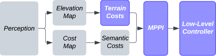
Figure 3: Information flow across perception and control. The focus of this work are highlighted in purple.

Our system can be abstracted into an upstream perception model, mid-level MPC planner, and a low-level controller (fig. 3). Our robotic platform is a modified Polaris RZR, fitted with LiDAR and RGB-D cameras as well as four NVIDIA GeForce RTX 3080 GPUs. Note the control algorithm utilizes only one of these GPUs.

IV-A Perception

The perception model receives data from the onboard sensors as input. At a rate of about 10 Hz, it outputs two grid-maps centered at the current location. One of these grid-maps provides semantic information about the environment (e.g. trees, grass, rocks) [37, 38, 39]. While terrain semantics affect vehicle dynamics, this paper is focused on utilizing information from the second grid-map: the elevation map. We refer readers to [40] for an in-depth description and evaluation of our perception system.

IV-B MPPI

IV-B1 Fast and Parallel Model Rollouts

We implement MPPI sampling, kinematic rollout, and cost function evaluation in a TorchScript PyTorch module running on an NVIDIA RTX 3080 GPU. Cost computations are vectorized across samples and the control horizon such that one iteration of MPPI samples are evaluated altogether in parallel. Our average MPPI computational time for one iteration is $29.6\pm 0.9$ ms or about $33.8$ Hz.

IV-B2 Cost Function

We evaluate costs of sampled kinematic rollouts against the elevation map. Our cost function is given by:

$$\small c(\mathbf{x},\mathbf{u})\coloneqq w_{1}c_{\text{rollover}}(\mathbf{x},\mathbf{u})+\,w_{2}c_{\text{airtime}}(\mathbf{x},\mathbf{u})+\,w_{3}c_{\text{bump}}(\mathbf{x},\mathbf{u})$$

where each $w_{i}$ is a hand-tuned weight, typically a large positive value.

Incorporating our rollover bound (4), the rollover cost term is a cumulative sum over the constraint violations,

$$\small c_{\text{rollover}}(\mathbf{x}_{t+h},\mathbf{u}_{t+h})\coloneqq\sum_{k=t}^{t+h}{RR}(k)\cdot\mathbf{1}\left\{{RR}(k)>{RR}_{\text{max}}\right\}$$ (8)

where,

$$\small{RR}(k)\coloneqq\frac{\left\lvert v_{k}^{2}\kappa_{k}-g\sin\phi(k)\right\rvert}{\cos\phi(k)}$$ (9)

and ${RR}_{\text{max}}\leq g\,{P}_{2}/{P}_{3}$ is the tunable parameter to control the vehicle’s aggressiveness with rollover risk.

For ditch handling, in addition to the maximum allowable torque magnitude $\tau_{\text{min}}^{\text{res}}$, we replace the upper bound from (7) with the parameter $\tau_{\text{max}}^{\text{res}}$ such that $\tau_{\text{max}}^{\text{res}}<0$. As the linear accelerations $\dot{v}_{t}$ sampled from MPPI can be noisy, we remove $\dot{v}_{t}$ from (7) to obtain a more tunable bound. We also compute $\omega_{2}$ and $\alpha_{2}$ through forward numerical differencing of $\theta(t)$. Our time-indexed $\tau_{\text{ditch}}^{\text{res}}$ can be computed as

$$\tau_{\text{ditch}}^{\text{res}}(t)=\bar{I}_{22}\alpha_{2}(t)+{P}_{1}v_{t}\omega_{2}(t)-{P}_{3}g\sin\theta(t)-{P}_{1}g\cos\theta(t)$$

For conciseness, define $\delta_{\text{min}}(t)\coloneqq\tau_{\text{min}}^{\text{res}}-\tau_{\text{ditch}}^{\text{res}}(t)$ and $\delta_{\text{max}}(t)\coloneqq\tau_{\text{ditch}}^{\text{res}}(t)-\tau_{\text{max}}^{\text{res}}$. As with rollover, we employ the cumulative sum of violations,

$$c_{\text{airtime}}(\mathbf{x}_{t+h},\mathbf{u}_{t+h}) \coloneqq\sum_{k=t}^{t+h}\delta_{\text{max}}(k)\cdot\mathbf{1}\left\{\delta_{\text{max}}(k)>0\right\}$$ (10)

$$c_{\text{bump}}(\mathbf{x}_{t+h},\mathbf{u}_{t+h}) \coloneqq\sum_{k=t}^{t+h}\delta_{\text{min}}(k)\cdot\mathbf{1}\left\{\delta_{\text{min}}(k)>0\right\}$$ (11)

IV-B3 Handling Control Delays

In practice, the issued control command $\hat{\mathbf{u}}_{t}$ can not be immediately executed on the vehicle due to software and hardware delays. This means that we actually have $\mathbf{x}_{t+1}=f(\mathbf{x}_{t},\hat{\mathbf{u}}_{t-\tau})$ for some delay $\tau\geq 0$. To handle delays, we consider the MPC optimization problem with a projected future state $\tilde{\mathbf{x}}_{t}$ rather than the true state $\mathbf{x}_{t}$. The projected future state $\tilde{\mathbf{x}}_{t}$ is given by rolling out the previously issued controls $(\hat{\mathbf{u}}_{t-\tau},\ldots,\hat{\mathbf{u}}_{t-1})$ starting from state $\mathbf{x}_{t}$. It effectively simulates the control commands that are issued but yet to be executed on the system.

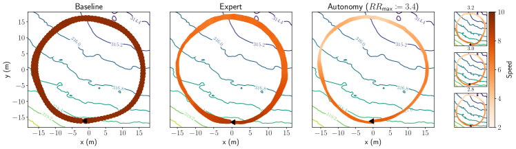
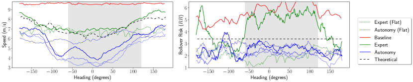
Figure 4: Top row. Spatial plot over elevation contour map of 15-meter radius circles on a 10-degree incline hill. Results for each experiment are averaged over at least five loops. Speed and $RR$ are reflected by the line color and marker width, respectively. Autonomy results of decreasing ${RR}_{\text{max}}$ control parameter are shown in the right column. Bottom row. Plots of speed and rollover risk as a function of heading angle. Off-camber turning highlighted by grey box. “Flat” results are collected from 15 m radius circles performed on flat ground. Theoretical max speed is calculated using ${RR}_{\text{max}}\coloneqq 3.4$. Opaquer autonomy lines correspond with higher ${RR}_{\text{max}}$ settings.

IV-B4 Sampling Control Sequences

The original MPPI algorithm samples the control sequences $\{\mathbf{u}_{t:t+H-1}^{i}\}_{i=1}^{N}$ from a Gaussian distribution centered around a nominal control sequence given by the shift operator [31, 28, 29, 27]. In our implementation, we sample raw control sequences $\{\tilde{\mathbf{u}}_{t:t+H-1}^{i}\}_{i=1}^{N}$ from a mixture of Gaussian distributions, and process the raw control sequences to generate sampled control sequences. When necessary, these Gaussians help the optimization with: (1) denser sampling around the nominal trajectory, (2) abrupt slow-downs, and (3) resetting local convergence on high-cost regions (see [41] for the explicit forms of these distributions).

Sampling feasible control sequences

The sampled changes in linear velocity and curvature must be limited due to the vehicle’s throttle, brake, and steering limitations. Additionally due to static friction, the steering is unchanged at linear velocities near zero.

We process the raw control sequences $\{\tilde{\mathbf{u}}_{t:t+H-1}^{i}\}_{i=1}^{N}$ so that feasibility constraints are satisfied. Let $\tilde{\mathbf{u}}_{t+h}^{i}=(\tilde{v}_{t+h}^{i},\tilde{\kappa}_{t+h}^{i})$, we iteratively compute the processed control sequence $\mathbf{u}_{t+h}^{i}=(v_{t+h}^{i},\kappa_{t+h}^{i})$,

$$\small\begin{split}v_{t+h}^{i}&=\mathrm{clip}(\tilde{v}_{t+h}^{i},v_{t+h-1}^{i}\pm\Delta v_{\max}),\\ \kappa_{t+h}^{i}&=\left\{\begin{array}[]{ll}\kappa_{t+h-1}^{i}&\text{if }|v_{t+h}^{i}|<v_{\min},\\ \mathrm{clip}(\tilde{\kappa}_{t+h}^{i},\kappa_{t+h-1}^{i}\pm\Delta\kappa_{\max})&\text{otherwise},\end{array}\right.\end{split}$$ (12)

where $\mathrm{clip}(a,b\pm c)\coloneqq{\max}({\min}(a,b+c),b-c)$ for $a,b,c\in\mathbb{R}$ and $c>0$. $\Delta v_{\max}$ and $\Delta\kappa_{\max}$ are the maximum changes of linear velocity and curvature, respectively, per time step, and $v_{\min}$ is the minimum speed that allows change of steering. We take $(v_{t-1}^{i},\kappa_{t-1}^{i})$ as the control issued at the previous step, $\hat{\mathbf{u}}_{t-1}$, for all $i$.

IV-C Low-Level Controller

We use a PI feedback controller with feedforward terms for drag and slope [42] to attain desired speeds from MPPI using throttle and brake:

$$u=-K_{P}(v-v_{t})-K_{I}\int(v-v_{t})dt+c_{1}g\sin\theta+c_{2}v$$

where $v_{t}$ is the desired linear velocity from MPPI, and $v$ is the actual velocity of the vehicle. The feedforward terms $c_{1}g\sin\theta+c_{2}v$ compensate for the acceleration in the $\mathbf{b}_{1}$ direction from gravity and the acceleration due to drag and friction. We determine the linear coefficients, $c_{1}$ and $c_{2}$ empirically from data and tune the proportional and integral gains $K_{P}$ and $K_{I}$. $u$ is then converted to throttle (when $u$ is positive) or brake (when $u$ is negative) using a pre-identified fixed mapping. Finally, for the steering angle, we directly translate the desired curvature $\kappa_{t}$ from MPPI to the steering angle command with a pre-identified fixed mapping.

V Results

Our experiments consist of two groups of tasks. One involves completing circles on slopes and is meant to test the robot’s ability to avoid rollovers. The second is crossing various ditches. With aggressive driving as our main goal, we benchmark the autonomy against an expert human driver who was instructed to drive as fast as possible in each task.

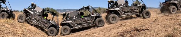
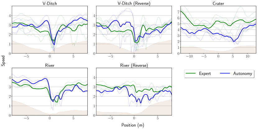
Figure 5: Robotic platform crossing the V-Ditch (pictured above). Average velocity is plotted as a function of the position through the ditch over the elevation profile (brown). Individual ditch traversals are plotted transparently.

V-A Rollover

We consider a baseline algorithm which uses a simplified cost of penalizing roll angles above $20$ degrees, similar to [8, 9, 10]. We compare the expert to the baseline in simulation (fig. 4). While the expert consistently operates at about ${RR}(t)\leq 6$, the baseline goes well above this threshold and in theory can surpass this arbitrarily due to its failure to consider dynamic effects. At ${RR}_{\text{max}}\approx 6$, the expert is experiencing slipping and tilting. This suggests that the baseline would roll the vehicle in the real world.

We also compare the expert to our method, the autonomy, with parameter ${RR}_{\text{max}}\coloneqq 3.4$ (fig. 4). For safety reasons, we do not autonomously operate the vehicle at ${RR}_{\text{max}}>3.4$. Still, we observe key similarities between the human expert and the behavior of our method. Like our method, the expert drives fastest through the on-camber turn and slowest through the off-camber turn (also observable in the “UW” slalom in fig. 1.3). A notable difference between the behaviors is how risk is managed. While the autonomy operates below the risk threshold with some margin, the expert anticipates the critical transition to off-camber turning by slowing down earlier. On the other hand, the quickly narrowing margin for the autonomy results in a sudden penalty and sharp slowdown.

We demonstrate our method’s ability to approach expert performance by varying ${RR}_{\text{max}}$ below our safety tolerance (fig. 4). Each increase in ${RR}_{\text{max}}$ trends towards more and more aggressive control.

V-B Ditches

Similar to the rollover task, we evaluate the autonomy in ditch crossing by comparing it with the expert (fig. 5). The tests are conducted over three distinct ditches with varying geometries.

In these experiments, the autonomy’s maximum speed was limited to 5 m/s for safety. With our approach, the autonomy executes similar speed profiles but runs at more conservative crossing speeds which can be attributed to our risk-adverse parameter tuning. Unlike the autonomy, the expert decelerates much earlier before the crossing. Note that the expert is familiar with the ditch geography and can anticipate the terrain. However, in practice, the descent angle of the ditch is often occluded from the vehicle’s view during the approach and can result in delayed sensing of the ditch geometry. This phenomenon likely contributes to the autonomy’s sharp decelerations in the V-Ditch and river crossings whose descent angles are initially occluded.

VI Conclusion

In this study, we propose a framework to augment 2D kinematic models with physics-based constraints for safe and aggressive off-road autonomous driving. This framework yields two constraints addressing failures due to rollover and unsafe ditch handling. Our control system design integrates this approach with a fast and efficient implementation of the MPPI algorithm. Finally, we validate our method through real-world experiments by autonomously traversing hills and ditches on our full-scale robotic platform. While these are isolated tests, we stress that the robot is not designed to perform them in isolation. We refer readers to the paper’s website for videos beyond our experiments for our general off-road performance.

By benchmarking against an expert driver, we observe similarities that demonstrate our approach’s ability to capture fundamental elements of safe yet aggressive control. Differences in the velocity profiles in our results suggest the importance of traction and uncertainty modeling for achieving performance closer to that of a human expert.

Appendix

VI-A Detailed Constraint Derivations

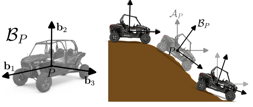
Figure 6: Body Frame on Vehicle

VI-A1 Acceleration Decomposition in Path Frame

As used in section III-B, the path frame as defined in [36] allows us to decompose the velocity $\mathbf{v}\coloneqq v\mathbf{b}_{1}$,

$$\mathbf{a} =\frac{d}{dt}\mathbf{v}=\frac{d}{dt}[v]\mathbf{b}_{1}+v\frac{d}{dt}[\mathbf{b}_{1}]$$

$$=\dot{v}\mathbf{b}_{1}+v\boldsymbol{\omega}\times\mathbf{b}_{1}$$ (13)

VI-A2 Rollover

Here, we expand on the derivation of (3). The residual torque from (2) can be combined with the decomposition from (13) and simplified such that

$$\boldsymbol{\tau}^{\text{res}}_{P}\cdot\mathbf{b}_{1} =\left[\mathbb{I}_{P}\cdot\boldsymbol{\alpha}-\mathbf{r}_{G/P}\times m\left(\mathbf{g}-\mathbf{a}\right)\right]\cdot\mathbf{b}_{1}$$

$$=-\left[\mathbf{r}_{G/P}\times m\left(\mathbf{g}-\mathbf{a}\right)\right]\cdot\mathbf{b}_{1}$$

$$=-\left[\mathbf{r}_{G/P}\times m(\mathbf{g}-\dot{v}\mathbf{b}_{1}-v\boldsymbol{\omega}\times\mathbf{b}_{1})\right]\cdot\mathbf{b}_{1}$$ (14)

Using vector product identities,

$$(\mathbf{r}_{G/P}\times\dot{v}\mathbf{b}_{1})\cdot\mathbf{b}_{1}=(\dot{v}\mathbf{b}_{1}\times\mathbf{b}_{1})\cdot\mathbf{r}_{G/P}=0$$

Also since $\mathbf{r}_{G/P}\cdot\mathbf{b}_{1}=0$,

$$\mathbf{r}_{G/P}\times(\boldsymbol{\omega}\times\mathbf{b}_{1}) =(\mathbf{r}_{G/P}\cdot\mathbf{b}_{1})\boldsymbol{\omega}-(\mathbf{r}_{G/P}\cdot\boldsymbol{\omega})\mathbf{b}_{1}$$

$$=-(\mathbf{r}_{G/P}\cdot\boldsymbol{\omega})\mathbf{b}_{1}$$

So, (14) simplifies as

$$\boldsymbol{\tau}^{\text{res}}_{P}\cdot\mathbf{b}_{1}=-m\left[\mathbf{r}_{G/P}\times\mathbf{g}+v(\mathbf{r}_{G/P}\cdot\boldsymbol{\omega})\mathbf{b}_{1}\right]\cdot\mathbf{b}_{1}$$

which gives us (3).

VI-B Explicit Forms of Gaussians for Control Sampling

• Conventional samples. The conventional samples are drawn from a Gaussian distribution centered at the nominal control sequences,

  $$\tilde{\mathbf{u}}_{t:t+H-1}^{\mathrm{conv}}\sim\mathcal{N}(\bar{\mathbf{u}}_{t:t+H-1},I_{H}\otimes\Sigma),\,\Sigma=\mathrm{diag}([\sigma_{1},\sigma_{2}]).$$

• Narrow samples. We find it to beneficial to sample more control sequences that are close to the nominal control sequence. Therefore, we sample a number of control sequences with a smaller covariance,

  $$\tilde{\mathbf{u}}_{t:t+H-1}^{\mathrm{narrow}}\sim\mathcal{N}(\bar{\mathbf{u}}_{t:t+H-1},I_{H}\otimes(s_{n}\cdot\Sigma)),$$

  with $s_{n}\in(0,1)$ being the narrow scaling coefficient.

• Scaled samples. We additionally sample around a scaled nominal control sequence which has smaller linear velocities. This allows the vehicle to effectively slow down while following a similar path as the nominal trajectory. Let $\bar{\mathbf{u}}_{t+h}=(\bar{v}_{t+h},\bar{\kappa}_{t+h}^{d})$ for any $h\in[0,H-1]$. We define the scaled nominal control sequence as

  $$\bar{\mathbf{u}}_{t:t+H-1}^{\mathrm{scaled}}\coloneqq((s_{s}\bar{v}_{t},\bar{\kappa}_{t}^{d}),\ldots,(s_{s}\bar{v}_{t+H-1},\bar{\kappa}_{t+H-1}^{d})),$$

  with $s_{s}\in(0,1)$ being scaling coefficients. The scaled samples are drawn from a Gaussian distribution centered at the scaled nominal control sequence,

  $$\tilde{\mathbf{u}}_{t:t+H-1}^{\mathrm{scaled}}\sim\mathcal{N}(\bar{\mathbf{u}}_{t:t+H-1}^{\mathrm{scaled}},I_{H}\otimes\Sigma).$$

• Reset samples. Finally, we include a small number of raw control sequences sampled from fixed-mean Gaussian distributions. These samples can reset the optimization if the nominal control sequence becomes high-cost due to, e.g., newly detected obstacles and terrain features.

  $$\tilde{\mathbf{u}}_{t:t+H-1}^{\textrm{reset},k}\sim\mathcal{N}(\mathds{1}_{H}\otimes\bar{\mathbf{u}}_{\mathrm{reset}}^{k},I_{H}\otimes\Sigma).$$

  In particular, we consider three fixed mean controls, $\mathbf{u}_{\mathrm{reset}}^{1}=(0,0)$, $\mathbf{u}_{\mathrm{reset}}^{2}=(0,-\kappa^{d}_{\max})$ and $\mathbf{u}_{\mathrm{reset}}^{3}=(0,\kappa^{d}_{\max})$, where $\kappa_{\max}^{d}$ is the maximum desired curvature. These fixed mean controls all uses zero linear velocity but have different desired curvatures.

References

- [1] Yugang Liu and Goldie Nejat. Robotic urban search and rescue: A survey from the control perspective. Journal of Intelligent & Robotic Systems, 72:147–165, 2013.
- [2] Hossein Mousazadeh. A technical review on navigation systems of agricultural autonomous off-road vehicles. Journal of Terramechanics, 50(3):211–232, 2013.
- [3] Daniel W Carruth, Clayton T Walden, Christopher Goodin, and Sara C Fuller. Challenges in low infrastructure and off-road automated driving. In 2022 Fifth International Conference on Connected and Autonomous Driving (MetroCAD), pages 13–20. IEEE, 2022.
- [4] Liang Ma, Jianru Xue, Kuniaki Kawabata, Jihua Zhu, Chao Ma, and Nanning Zheng. Efficient sampling-based motion planning for on-road autonomous driving. IEEE Transactions on Intelligent Transportation Systems, 16(4):1961–1976, Aug 2015.
- [5] Brian Paden, Michal Čáp, Sze Zheng Yong, Dmitry Yershov, and Emilio Frazzoli. A survey of motion planning and control techniques for self-driving urban vehicles. IEEE Transactions on Intelligent Vehicles, 1(1):33–55, Mar 2016.
- [6] Jianjun Du, Mingjun Ren, Jianjun Zhu, and Dun Liu. Study on the dynamics and motion capability of the planetary rover with asymmetric mobility system. In The 2010 IEEE International Conference on Information and Automation, page 682–687, Jun 2010.
- [7] Yunbo Zhou and Xianhui Wang. Obstacle performance simulation of tracked vehicles based on the adams/atv. In Proceedings 2011 International Conference on Transportation, Mechanical, and Electrical Engineering (TMEE), page 783–786, Dec 2011.
- [8] Aniket Datar, Chenhui Pan, and Xuesu Xiao. Learning to model and plan for wheeled mobility on vertically challenging terrain. arXiv preprint arXiv:2306.11611, 2023.
- [9] David D Fan, Kyohei Otsu, Yuki Kubo, Anushri Dixit, Joel Burdick, and Ali-Akbar Agha-Mohammadi. Step: Stochastic traversability evaluation and planning for risk-aware off-road navigation. arXiv preprint arXiv:2103.02828, 2021.
- [10] Philipp Krüsi, Paul Furgale, Michael Bosse, and Roland Siegwart. Driving on point clouds: Motion planning, trajectory optimization, and terrain assessment in generic nonplanar environments. Journal of Field Robotics, 34(5):940–984, 2017.
- [11] Ronald L Huston and Fred A Kelly. Another look at the static stability factor (ssf) in predicting vehicle rollover. International journal of crashworthiness, 19(6):567–575, 2014.
- [12] Jia-Ern Pai. Trends and rollover-reduction effectiveness of static stability factor in passenger vehicles. Technical report, 2017.
- [13] M. Doumiati, A. Victorino, A. Charara, and D. Lechner. Lateral load transfer and normal forces estimation for vehicle safety: experimental test. Vehicle System Dynamics, 47(12):1511–1533, Dec 2009.
- [14] Chad Larish, Damrongrit Piyabongkarn, Vasilios Tsourapas, and Rajesh Rajamani. A new predictive lateral load transfer ratio for rollover prevention systems. IEEE Transactions on Vehicular Technology, 62(7):2928–2936, Sep 2013.
- [15] PJ Liu, S Rakheja, and AKW Ahmed. Detection of dynamic roll instability of heavy vehicles for open-loop rollover control. SAE transactions, pages 632–639, 1997.
- [16] Selim Solmaz, Martin Corless, and Robert Shorten. A methodology for the design of robust rollover prevention controllers for automotive vehicles with active steering. International Journal of Control, 80(11):1763–1779, 2007.
- [17] Antonio Tota, Luca Dimauro, Filippo Velardocchia, Genny Paciullo, and Mauro Velardocchia. An intelligent predictive algorithm for the anti-rollover prevention of heavy vehicles for off-road applications. Machines, 10(1010):835, Oct 2022.
- [18] Bo-Chiuan Chen and Huei Peng. Differential-braking-based rollover prevention for sport utility vehicles with human-in-the-loop evaluations. Vehicle system dynamics, 36(4-5):359–389, 2001.
- [19] H Dahmani, M Chadli, A Rabhi, and A El Hajjaji. Vehicle dynamic estimation with road bank angle consideration for rollover detection: theoretical and experimental studies. Vehicle System Dynamics, 51(12):1853–1871, 2013.
- [20] Brian César-Tondreau, Garrett Warnell, Kevin Kochersberger, and Nicholas R Waytowich. Towards fully autonomous negative obstacle traversal via imitation learning based control. Robotics, 11(4):67, 2022.
- [21] Xingyu Li, Bo Tang, John Ball, Matthew Doude, and Daniel W. Carruth. Rollover-free path planning for off-road autonomous driving. Electronics, 8(66):614, Jun 2019.
- [22] Siyuan Yu, Congkai Shen, and Tulga Ersal. Nonlinear model predictive planning and control for high-speed autonomous vehicles on 3d terrains. IFAC-PapersOnLine, 54(20):412–417, Jan 2021.
- [23] Qifan Tan, Cheng Qiu, Jing Huang, Yue Yin, Xinyu Zhang, and Huaping Liu. Path tracking control strategy for off-road 4ws4wd vehicle based on robust model predictive control. Robotics and Autonomous Systems, 158:104267, Dec 2022.
- [24] Jason Gibson, Bogdan Vlahov, David Fan, Patrick Spieler, Daniel Pastor, Ali-akbar Agha-mohammadi, and Evangelos A. Theodorou. A multi-step dynamics modeling framework for autonomous driving in multiple environments. (arXiv:2305.02241), May 2023. arXiv:2305.02241 [cs, eess].
- [25] Samuel Triest, Matthew Sivaprakasam, Sean J Wang, Wenshan Wang, Aaron M Johnson, and Sebastian Scherer. Tartandrive: A large-scale dataset for learning off-road dynamics models. In 2022 International Conference on Robotics and Automation (ICRA), pages 2546–2552. IEEE, 2022.
- [26] Xuesu Xiao, Joydeep Biswas, and Peter Stone. Learning inverse kinodynamics for accurate high-speed off-road navigation on unstructured terrain. IEEE Robotics and Automation Letters, 6(3):6054–6060, 2021.
- [27] N Wagener, C Cheng, J Sacks, and B Boots. An online learning approach to model predictive control. In Proceedings of Robotics: Science and Systems (RSS), 2019.
- [28] Grady Williams, Nolan Wagener, Brian Goldfain, Paul Drews, James M Rehg, Byron Boots, and Evangelos A Theodorou. Information theoretic mpc for model-based reinforcement learning. In 2017 IEEE International Conference on Robotics and Automation (ICRA), pages 1714–1721. IEEE, 2017.
- [29] Mohak Bhardwaj, Balakumar Sundaralingam, Arsalan Mousavian, Nathan D Ratliff, Dieter Fox, Fabio Ramos, and Byron Boots. Storm: An integrated framework for fast joint-space model-predictive control for reactive manipulation. In Conference on Robot Learning, pages 750–759. PMLR, 2021.
- [30] Jason Kong, Mark Pfeiffer, Georg Schildbach, and Francesco Borrelli. Kinematic and dynamic vehicle models for autonomous driving control design. In 2015 IEEE Intelligent Vehicles Symposium (IV), page 1094–1099, Jun 2015.
- [31] Grady Williams, Andrew Aldrich, and Evangelos A Theodorou. Model predictive path integral control: From theory to parallel computation. Journal of Guidance, Control, and Dynamics, 40(2):344–357, 2017.
- [32] Péter Fankhauser, Michael Bloesch, and Marco Hutter. Probabilistic terrain mapping for mobile robots with uncertain localization. IEEE Robotics and Automation Letters, 3(4):3019–3026, Oct 2018.
- [33] Bianca Forkel and Hans-Joachim Wuensche. Dynamic resolution terrain estimation for autonomous (dirt) road driving fusing lidar and vision. In 2022 IEEE Intelligent Vehicles Symposium (IV), page 1181–1187, Aachen, Germany, Jun 2022. IEEE Press.
- [34] Maximilian Stölzle, Takahiro Miki, Levin Gerdes, Martin Azkarate, and Marco Hutter. Reconstructing occluded elevation information in terrain maps with self-supervised learning. IEEE Robotics and Automation Letters, 7(2):1697–1704, Apr 2022.
- [35] Rudolph Triebel, Patrick Pfaff, and Wolfram Burgard. Multi-level surface maps for outdoor terrain mapping and loop closing. In 2006 IEEE/RSJ International Conference on Intelligent Robots and Systems, page 2276–2282, Beijing, China, Oct 2006. IEEE.
- [36] Jeremy Kasdin and Derek Paley. Engineering Dynamics. Mar 2011.
- [37] Kashyap Chitta, Aditya Prakash, and Andreas Geiger. Neat: Neural attention fields for end-to-end autonomous driving. In 2021 IEEE/CVF International Conference on Computer Vision (ICCV), page 15773–15783, Montreal, QC, Canada, Oct 2021. IEEE.
- [38] Alonzo Kelly, Anthony Stentz, Omead Amidi, Mike Bode, David Bradley, Antonio Diaz-Calderon, Mike Happold, Herman Herman, Robert Mandelbaum, Tom Pilarski, Pete Rander, Scott Thayer, Nick Vallidis, and Randy Warner. Toward reliable off road autonomous vehicles operating in challenging environments. The International Journal of Robotics Research, 25(5–6):449–483, May 2006.
- [39] Amirreza Shaban, Xiangyun Meng, JoonHo Lee, Byron Boots, and Dieter Fox. Semantic terrain classification for off-road autonomous driving. In Aleksandra Faust, David Hsu, and Gerhard Neumann, editors, Proceedings of the 5th Conference on Robot Learning, volume 164 of Proceedings of Machine Learning Research, pages 619–629. PMLR, 08–11 Nov 2022.
- [40] Xiangyun Meng, Nathan Hatch, Alexander Lambert, Anqi Li, Nolan Wagener, Matthew Schmittle, JoonHo Lee, Wentao Yuan, Zoey Chen, Samuel Deng, et al. Terrainnet: Visual modeling of complex terrain for high-speed, off-road navigation. arXiv preprint arXiv:2303.15771, 2023.
- [41] Off-Road MPC. Model predictive control for aggressive driving over uneven terrain. https://sites.google.com/cs.washington.edu/off-road-mpc/home, 2023. Accessed: 2023-08-22.
- [42] Guanya Shi, Wolfgang Hönig, Xichen Shi, Yisong Yue, and Soon-Jo Chung. Neural-swarm2: Planning and control of heterogeneous multirotor swarms using learned interactions. IEEE Transactions on Robotics, 38(2):1063–1079, 2021.