Geometric Characterization of Many Body Localization

Abstract

Many body localization (MBL) represents a unique physical phenomenon, providing a testing ground for exploring thermalization, or more precisely its failure. Here we characterize the MBL phase geometrically by the many-body quantum metric (MBQM), defined in the parameter space of twist boundary. We find that MBQM scales linearly as a function of the inverse system length in the MBL phase, and grows faster in the ergodic phase. We validate our theory using the disordered hardcore Bose-Hubbard model, and characterize the ergodic to MBL phase transition via the localization length scale defined from the MBQM. MBQM provides an intuitive and experimentally accessible method to characterize MBL phases.

Advancements in highly controllable experimental platforms, such as optical lattices[1, 2, 3, 4], trapped ions[5], and Rydberg atom arrays[6, 7], have allowed for realizations of well isolated quantum systems in the lab where quantum dynamics and non equilibrium physics can be observed [8, 9]. Of particular interest are nonergodic systems, which do not thermalize within a finite time. These systems can host stable phases of matter and help to understand thermalization mechanisms [10]. Thus far the only known robust nonergodic phase is many body localization (MBL), which arises from the interplay of disorder and interactions [11, 12]. In contrast, other nonergodic phases, such as non-interacting phases, quantum scars or integrable models, typically thermalize with the addition of some perturbation [13].

Anderson localization was the first identified nonergodic system wherein disorder in a non-interacting system localizes all eigenstates [14]. Following studies saw the inclusion of interactions to determine the stability of the ground state in this localized phase, finding that indeed localization persisted in several regimes [15, 16, 17]. More recent studies have found that excited states, even those corresponding to infinite temperature, can remain localized, resulting in a phenomenon termed MBL [18, 19, 20].

MBL hosts many interesting properties beyond those observed in its non-interacting counterpart and demonstrates a unique dynamical phase transition between the localized and delocalized regions. The phase boundary can be determined through the entanglement entropy scaling as a function of system size, as in the delocalized region entanglement entropy grows with volume while in the localized phase the entanglement follows an area law [21]. Additionally the entanglement entropy growth of initial product states has been shown to grow logarithmically, in contrast to the quickly saturating entanglement entropy in non-interacting Anderson insulators [22]. The unique behavior of the entanglement entropy is related to the localization that occurs in Fock space in addition to the real space localization. This has been shown to be related to the emergence of a set of quasilocal integrals of motion (LIOM), which has allowed for the construction of phenomenological models of MBL[23]. Strong evidence of MBL has been found in the disordered Bose-Hubbard [24, 25] and Fermi-Hubbard models [26] in 1D as well as quasi-disordered lattice systems with non commensurate periodic external potentials [27].

An important parameter in understanding insulating states is the characteristic localization length. To present, there have been several proposed approaches to extracting the localization length in MBL systems. For example, a localization length can be defined in terms of the inverse participation ratio obtained from the single particle density matrix [28]. Other methods rely on phenomenological models constructed from the extensive set of LIOM, which introduces a hierarchy of length scales[29, 30]. The LIOM have been constructed explicitly for the XXZ model [31], the dirsordered hardcore Fermi-Hubbard model [32, 33], and the Heisenberg model[34]. Although there are several different localization lengths that appear in MBL, their physical meaning or experimental signature is often unclear.

A natural localization length has been defined in the modern theory of insulators, built upon the theory of polarization [35, 36, 37, 38, 39, 40]. In the modern theory of the insulator, the conductivity of a state is related to the variance in the position as defined in periodic systems to be the so-called many-body quantum metric (MBQM). If in the thermodynamic limit the MBQM diverges, then the system is a conductor while if it saturates the state is an insulator. This has been applied in several paradigmatic contexts, including quantum Hall insulators[41], Mott insulators[42], and Chern insulators[43]. MBQM is also experimentally observable through the response of the system upon a periodic modulation [44].

In this work, we discuss that a natural characteristic length scale for localization in real space can be defined through the MBQM in the MBL phase. We find that the MBQM in MBL phase depends linearly on $1/N$, where $N$ is the number of particles, whereas it depends more rapidly on $1/N$ in the ergodic phase. By extrapolating MBQM to the thermodynamic limit, we can extract a characteristic localization length. We calculate the MBQM as a function of interaction and disorder strength to construct a phase diagram of the disordered hardcore Bose-Hubbard model.

The many-body quantum metric (MBQM) - The MBQM is a geometrical property of many-body quantum states defined in the parameter space of twisted boundary conditions. We focus on one-dimensional systems in this paper. Having a twisted boundary condition with phase $\theta$ is equivalent to having a flux $\theta$ inserted through the system with the wavefunction obeying the periodic boundary condition without twist [45]. Let us denote the Hamiltonian of the system with a flux $\theta$ inserted by $H(\theta)$. The MBQM, which we denote by $g(\theta)$, for a state $|\phi_{0}\rangle$, is then defined as [46, 47]

$$g(\theta)=\sum_{n\neq 0}\frac{\langle\phi_{0}|\partial_{\theta}H(\theta)|\phi_{n}\rangle\langle\phi_{n}|\partial_{\theta}H(\theta)|\phi_{0}\rangle}{(E_{0}-E_{n})^{2}},$$ (1)

where the sum is over all the eigenstates $|\phi_{n}\rangle$, whose corresponding eigenenergies are $E_{n}$, which are different from the state under consideration, $|\phi_{0}\rangle$. (We note that both $|\phi_{n}\rangle$ and $E_{n}$ depend on $\theta$ in general.) The MBQM has been used to characterize conductor-insulator transitions as in the thermodynamic limit, it goes to a fixed value in an insulator while it diverges in a conductor [37, 48]. This difference in the bahavior of the MBQM for conductors and insulators motivates us to characterize the MBL using MBQM. When the system is large enough, we can expect that $g(\theta)$ does not depend on $\theta$ following arguments similar to those in Refs. [45, 37, 49]; we will thus consider MBQM at $\theta=0$ in the following discussion without loss of generality.

The behavior of the $g$ in the localized and delocalized regime displays markedly different scaling properties. When the wavefunction is fully localized within a finite region in a space, one can show that $g=\mathrm{Var}(X_{CM})/L^{2}$ for a system with length $L$ and $X_{CM}\equiv\sum_{n}x_{n}$ with $x_{n}$ the position operator for the $n$-th particle [37]. Here we use the notation that for variables $X_{1}$ and $X_{2}$, the variance is defined by $\text{Var}(X_{1}):=\langle X_{1}^{2}\rangle-\langle X_{1}\rangle^{2}$ and the covariance, which we use later, is defined as $\text{Cov}(X_{1},X_{2}):=\langle X_{1}X_{2}\rangle-\langle X_{1}\rangle\langle X_{2}\rangle$ where the brackets correspond to the expectation value.

When the wavefunction is not fully localized in a finite region, defining the position operator $X_{CM}$ under the periodic boundary condition is a tricky issue, but $L^{2}g$ can still be used to represent $\mathrm{Var}(X_{CM})$, or the second cumulant of $X_{CM}$, as discussed in detail in [37]. We are then tempted to write, by the indistinguishability of particles,

$$L^{2}g=\text{Var}(X_{CM})\sim\sum_{i,j}\left(\langle x_{i}x_{j}\rangle-\langle x_{i}\rangle\langle x_{j}\rangle\right)$$

$$\sim N^{2}\left(\left[\text{Var}(x_{1})-\text{Cov}(x_{1},x_{2})\right]/N+\text{Cov}(x_{1},x_{2})\right).$$ (2)

However, we note that this equation is not rigorously established, as we have not defined the position operator $x_{i}$ for the $i$-th particle in the periodic boundary condition. Rather, we can use the equation Eq. (2) as a guiding principle to understand the scaling behavior of $g$ in large $N$ limit when one is in MBL phase where variance and covariance of particle positions are expected to take finite values. What Eq. (2) suggests, which we indeed later numerically confirm, is that $L^{2}g/N^{2}$ scales linearly in $1/N$ with a constant offset term, analogous to $\text{Cov}(x_{1},x_{2})$. On the other hand, if one is in ergodic region, we cannot expect the variance of particle positions to remain finite, and thus we cannot expect $L^{2}g/N^{2}$ to scale linearly in $1/N$. We shall see later that the $1/N$ dependence of $L^{2}g/N^{2}$ in the ergodic phase is much more rapid than that in the MBL phase.

The Disordered hardcore Bose-Hubbard model - As a concrete example, we use the disordered hardcore Bose-Hubbard model at half-filling to explore the relation between the MBQM and ergodic-MBL phase transition. The Hamiltonian is given by

$$H=-t\sum_{j}a^{\dagger}_{j+1}a_{j}+a^{\dagger}_{j}a_{j+1}+\sum_{j}\mu_{j}n_{j}+U\sum_{j}n_{j}n_{j+1}$$ (3)

where $a^{\dagger}_{j},a_{j}$ are Bosonic creation and annihilation operators on site $j$ and $n_{j}=a^{\dagger}_{j}a_{j}$ is the density operator. The parameters $t$ and $U$ control the hopping and nearest neighbor interaction strengths, respectively, and $\mu_{j}$ is the disordered onsite potential taken from a random uniform distribution on the interval $[-W,W]$. This model has been shown to host an MBL phase in limit of large disorder [50]. We will fix $t=1$ and study the phase diagram as a function of $U$ and $W$. For evaluation of the MBQM as defined in Eq. 1, the required derivative is

$$\left.\partial_{\theta}H(\theta)\right|_{\theta=0}=-\frac{it}{L}\sum_{j}a^{\dagger}_{j+1}a_{j}-a^{\dagger}_{j}a_{j+1}$$ (4)

obtained by taking periodic boundary conditions and threading a flux $\theta$.

The MBQM for One Particle - Before considering the full problem at half-filling, let us demonstrate the relation between the MBQM and the localization for a single particle. When there is only one particle, the disordered Bose-Hubbard model is just the Anderson model, where all the eigenstates are localized for any disorder strength $W$. As stated previously, the MBQM is related to the variance of the particle as $L^{2}g=\text{Var}(x)$, when the wavefunction is localized. To understand the behavior of $L^{2}g$ when the wavefunction is not localized, we calculate $L^{2}g$ for various lengths and disorder strengths for the Anderson model. For a given disorder realization, we calculate single-particle eigenstates and calculate $L^{2}g$ for a randomly selected state. We repeat the procedure for $10^{6}$ realizations and take the median value of $L^{2}g$. (We can also take the average here, instead of the median; for the MBL phase at half filling, however, as we discuss below, we find that median converges much faster than the average.) In Fig 1, we plot the median of $L^{2}g$, for system sizes $L=30,40,50$ and $60$ versus the disorder strength $W$. We find that above approximately a disorder strength of $W\sim 1$, values of $L^{2}g$ for different lengths match, and agree with the directly calculated values of $\text{Var}(x)$ assuming the open boundary . On the other hand, below the disorder $W\sim 1$, we observe that $L^{2}g$ varies with the system length, and they also deviate from $\text{Var}(x)$ calculated under the open boundary condition. The deviation between $L^{2}g$ and $\text{Var}(x)$ happen at smaller values of $W$ for systems with longer $L$. This length dependence of $L^{2}g$ and discrepancy between $L^{2}g$ and $\text{Var}(x)$ are attributed to the eigenstates touching the boundary at smaller values of $W$; when the wavefunction is spread over the entire finite-sized chain, $\text{Var}(x)$ calculated under the open boundary condition and $L^{2}g$ do not need to coincide. We note that, although $L^{2}g$ loses its direct meaning as $\text{Var}(x)$ when the wavefunction is extended, it is a perfectly well-defined quantity both in the localized and extended region. An important observation here is that $L^{2}g$ do not depend on the system size in the localized region, whereas it depends on the system size in the delocalized region. We confirm similar behavior of the system-size dependence of MBQM for two-particle systems, as discussed in detail in the Supplemental Material. We will see below that similar behavior holds for disordered Bose-Hubbard model at half filling; $L^{2}g/N^{2}$ has weak dependence on $L$ in the MBL phase whereas it depends on $L$ more strongly in the ergodic phase.

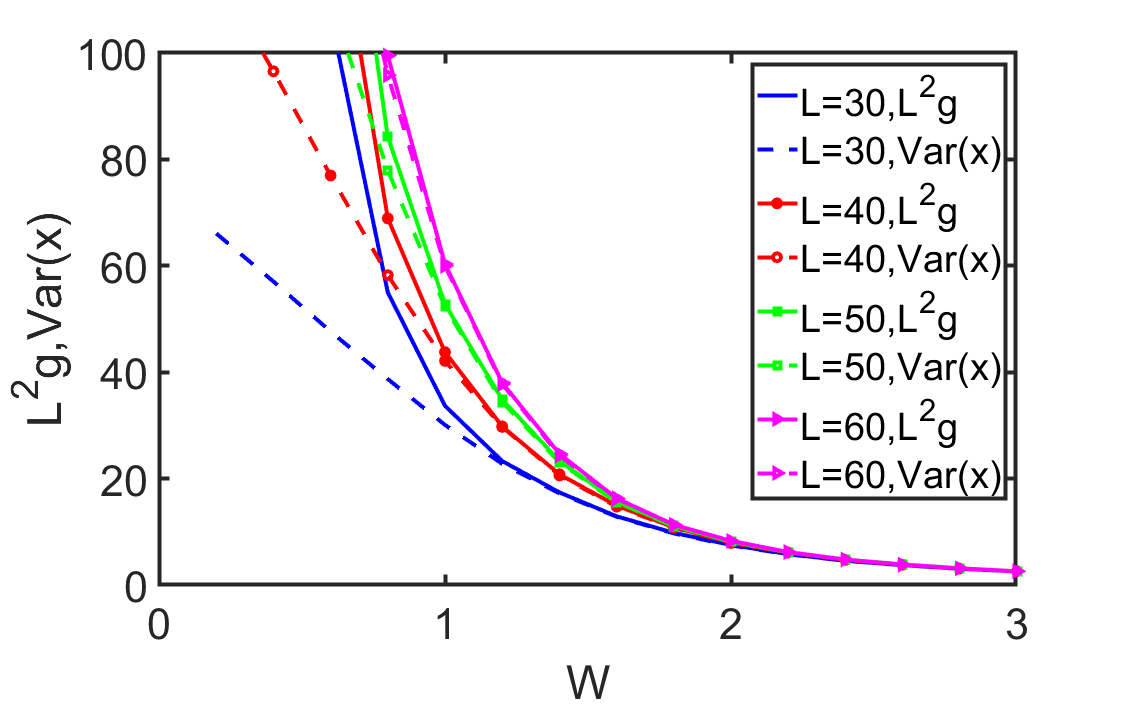
Figure 1: MBQM ($L^{2}g$) as a function of the disorder strength $W$ for single particle systems with different system lengths $L$. The plotted values are the median of $10^{6}$ disorder realizations. Dashed lines are the medians of $\text{Var}(x)$ calculated assuming the open boundary condition. These quantities agree when the disorder strength is larger than approximately $W\sim 1$, which corresponds to the region with well localized wavefunction, and agreement improves as the system size increases.

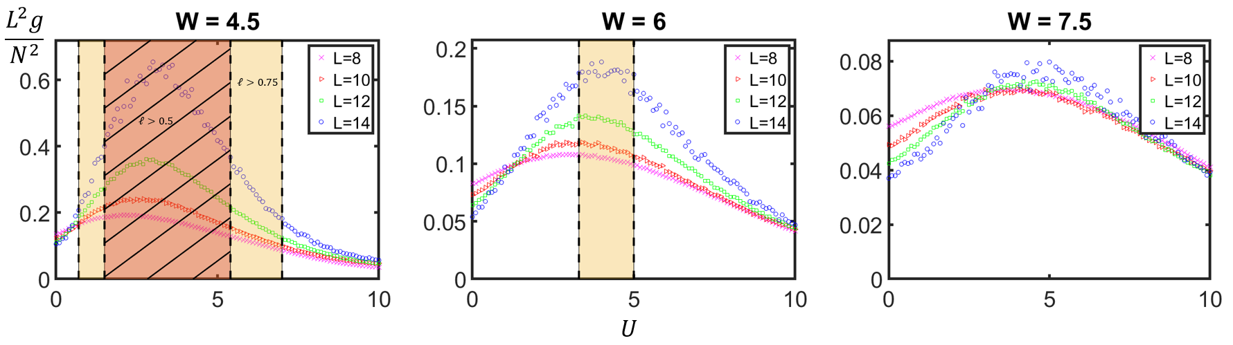
Figure 2: Median MBQM ($L^{2}g/N^{2}$) as a function of interaction strength $U$ for different disorder strengths and different system sizes. Disorder strengths from left to right are $W=4.5$, 6.0, and 7.5. The shadings correspond to regions where the quantity $\ell=\lim_{N\to\infty}L\sqrt{g}/N$ is greater than the proposed cutoff as labelled on the plot for $W=4.5$.

Bose-Hubbard model at Half-filling - Now we consider the MBQM of the half-filled disordered Bose-Hubbard model. In our calculation we shift the energies to $E-(E_{max}+E_{min})/2$ and consider the state with energy closest in magnitude to 0, which corresponds to infinite temperature in the thermodynamic limit. Here $E_{max}$ and $E_{min}$ are the largest and lowest eigenenergies in the spectrum of a given disorder realization, respectively. We perform computation over $10^{5}$ disorder realizations for $L=8$, $10^{4}$ realizations for $L=10,12$, and $10^{3}$ realizations for $L=14$. We consider the median of the disorder as the average does not always converge within these number of realizations due to the appearance of configurations with anomalously high MBQM, resulting from accidental near degeneracies. We note that, at half filling, the many-body wavefunction is always spread over the entire system; we show in Supplemental Material that the density distribution is indeed nonzero on all sites for typical states, even in the MBL phase. We will show that MBQM, extrapolated to the thermodynamic limit, nonetheless provides a meaningful characteristic localization length.

In Fig. 2, we present the median MBQM, scaled as $L^{2}g/N^{2}$, as a function of interaction strength for different system sizes. We note that at half filling, $N/L=1/2$, which means that $L^{2}g/N^{2}=4g$. We choose to explicitly write as $L^{2}g/N^{2}$ in this section, rather than $4g$, to show its $L$ and $N$ dependence. Each panel corresponds to a different disorder strength. We see that, for $W=4.5$ and 6, $L^{2}g/N^{2}$ has weak dependence on $L$ at small and large values of $U$ while it grows much more rapidly with $L$ at the medium values of $U$. For $W=7.5$, $1/N$ dependence of $L^{2}g/N^{2}$ always seems to be weak. Previous works have found that this model shows MBL both at small and large values of $U$ when $W$ is not too large, and enters into ergodic phase at the intermediate values of $U$. When $W$ is large, the ergodic phase does not appear [52, 53]. We can thus identify the region where $L^{2}g/N^{2}$ depends weakly on $L$ as the MBL phase, and the region with strong $L$ dependence as the ergodic phase; we will later show more quantitative comparison of the phase diagram with the existing theory of MBL. We note that the strong system size dependence of $L^{2}g/N^{2}$ in the ergodic phase is reminiscent of the behavior of entanglement entropy previously observed [21]. The shadings in Fig. 2 correspond to different proposed phase boundaries that we explain below.

The re-entrant MBL phase transition as $U$ is increased further beyond the ergodic phase has been found in earlier works [26, 52, 53]. To our knowledge, no property to distinguish the MBL phases at small and large $U$ in the hardcore Bose-Hubbard model has been found, but there have been proposals of MBL phases with different clustering properties when the hardcore constraint is relaxed [54]. Here we find that the scaling behavior of $L^{2}g/N^{2}$ can distinguish the two phases; for low $U$, $L^{2}g/N^{2}$ grows with system size whereas for large $U$, $L^{2}g/N^{2}$ decreases with the system size. Our finding suggests that the mechanisms behind the MBL phase in small and large $U$ regimes have different origins.

We now quantify the scaling behavior of the MBQM by fitting $1/N$ dependence of $L^{2}g/N^{2}$, which from Eq. 2 we expect to scale linearly in the MBL phase. In Fig 3, we present two such example fittings in the ergodic (left) and MBL (right) phases to illustrate their differences. In the MBL phase, linear fitting well approximates the numerically obtained $L^{2}g/N^{2}$ for four different values of $N$, and quadratic fitting does not improve the fitting very much. On the other hand, in the ergodic phase, linear fitting and quadratic fitting yield a big difference. Furthermore, from the slope of the fit we observe that $1/N$ dependence in the MBL regime is much weaker than that in the ergodic regime, confirming the finding from Fig. 2. In Fig. 3, we chose cases where the difference in fitting behaviors between the ergodic and MBL phases is visibly apparent. More generally, it is not always easy to find the difference in the ergodic and MBL phases by eye. We have thus developed a more quantitative way to analyze the difference between the linear and quadratic fittings through their least squared residuals. We find that the fitting residuals between linear and quadratic fits is qualitatively smaller in the MBL regime than in the ergodic regime; more detailed analysis on linear and quadratic fittings is provided in the Supplemental Material. The accuracy of our analysis is limited by the few number of system sizes achievable with exact diagonalization; better quantitative comparison between linear and quadratic fits is possible if simulation, or experimental realization, with longer system sizes is available.

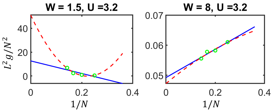
Figure 3: Linear and quadratic fittings of $L^{2}g/N^{2}$ as a function of $1/N$ in the extended (left) and MBL (right) phases. Blue solid (red dashed) lines correspond to linear (quadratic) fitting.

From Eq. (2), we expect $L^{2}g/N^{2}$ to scale linearly in $1/N$ in the MBL phase, which has been confirmed by the numerical results presented in Figs. 2 and  3 above. Taking the linear thermodynamic limit, we can define the quantity

$$\ell=\lim_{N\to\infty}L\sqrt{g}/N.$$ (5)

which in the MBL phase can be considered a localization, analogous to the positional covariance, $\text{Cov}(x_{1},x_{2})$. We have calculated and plotted $\text{log}_{10}\ell$in the $U-W$ plane in Fig. 4. Fixing the interaction strength $U$, and increasing the disorder $W$, we see that $\ell$ decreases, showing stronger localization as $W$ increases. For fixed disorder $W$, the behavior is more subtle; as $U$ is increased, $\ell$ increases first, showing that the system delocalizes, but after some maximum value, $\ell$ starts to decrease showing re-entrant localization transition.

To illustrate that we can determine a phase boundary from $\ell$ similar to those previously proposed, we plot several contours corresponding to $\ell=0.25$, 0.5, 0.75, and 1.0 alongside a dotted phase boundary according to the method given in Ref. [26]. Given the crossover nature of the transition between the two phases, we cannot draw a definitive phase boundary between the phases. Nonetheless, identifying the length scale $\ell$ to be a characteristic localization length, it is reasonable to assume $\ell$ in the MBL phase to be somewhat around or less than the lattice spacing at half filling. Indeed we find that the contours corresponding to 0.75 and 0.5 match quite well with the phase boundary previously found from the eigenvalue spacing statistics in Ref. [26], supporting our argument that the phase transition can be captured by the MBQM. (A complementary phase diagram based on fitting residuals is presented in the Supplemental Material.) In Fig. 5, we present $\ell$ as a function of interaction strength for three disorder strengths to further elucidate the trends observed in our phase diagram. Shadings again correspond to the different boundaries based on the contours in the phase diagram.

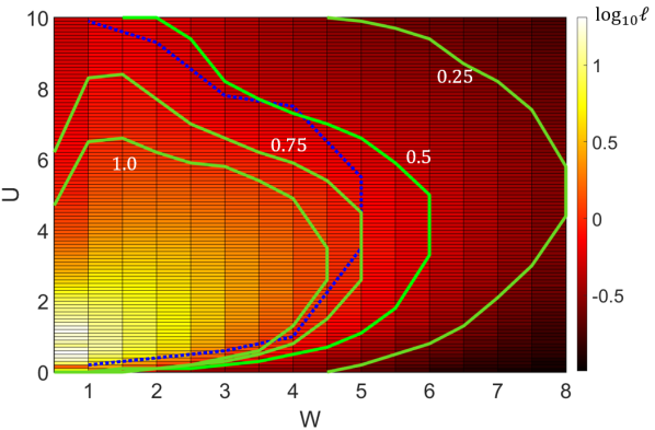
Figure 4: The MBL phase diagram: log of the characteristic length, $\log_{10}\ell$, plotted as a function of interaction $U$ and the disorder strength $W$. Solid green curves are labelled with the contour of equal values of $\ell$. The dotted blue contour corresponds to the predicted phase diagram in Ref. [26], demonstrating that $\ell\approx 0.5$ or 0.75 sets the boundary between the ergodic and MBL phases.

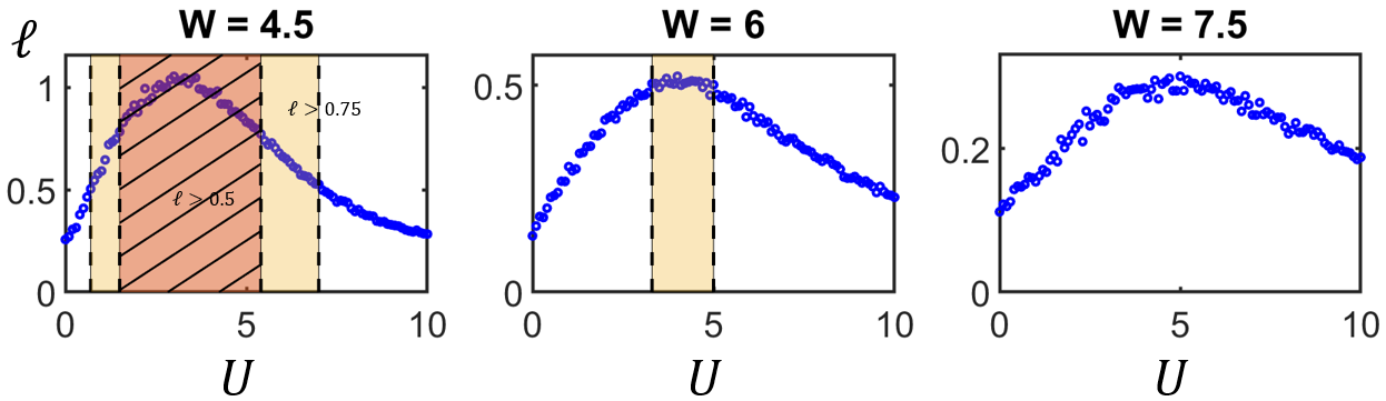
Figure 5: Characteristic localization length $\ell$ as a function of the interaction strength $U$ for three disorder strengths. Shaded region correspond to the ergodic phases determined by the cutoff $\ell=0.5$ or 0.75.

Conclusion - To summarize, we have shown that the system size dependence and the thermodynamic limit of MBQM provide an excellent means to distinguish the MBL phase from ergodic phase for the disordered Bose-Hubbard model. In particular, $\ell\equiv\lim_{N\to\infty}L\sqrt{g}/N$ provides a natural length scale to characterize the localized phase. The scaling behavior is reminiscent of the entanglement entropy scaling and the resulting phase boundaries agree with those previously proposed from other properties of the MBL.

The MBQM offers insight into further understanding the MBL phase. Experimentally it has been proposed that the MBQM can be extracted from the participation ratio in a lattice shaking experiment [44]. The MBQM should allow for a straightforward and general method for detecting the presence of MBL in a variety of systems, including fermionic and spin systems as well as MBL systems in the absence of disorder. Moving beyond exact diagonalozation methods to calculate the MBQM for larger systems will allow for improved accuracy in determining the phase boundary as we expect our localization length to scale completely differently in the two phases. In higher dimensions, the MBQM has a tensorial structure reflecting the localization of many-body quantum systems in different directions; such a higher dimensional MBQM may be able to determine the fate of MBL in higher dimensions.

I Acknowledgements

We thank Ryusuke Hamazaki and Henning Schomerus for discussions on many-body localization. This work has been supported by JSPS KAKENHI Grant Number JP20H01845, JST PRESTO Grant No. JPMJPR2353, JST CREST Grant Number JPMJCR19T1.

II Supplementary Material

II.1 Two Particle Results

As in the single particle case, MBQM ($L^{2}g$) and the variance of center-of-mass position of two particles agree when the wavefunction is well localized in real space. In Fig 6, we plot the median of the MBQM and the variance in the center of mass vs the interaction strength $U$ for two different disorder strengths. We see that the MBQM and variance agree well so long as the system is large enough and the disorder is strong enough, suggesting that we can attribute this discrepancy to finite size effects in complete agreement with the single particle results.

We now extract the single particle variance, $\text{Var}(x_{1})$ and covariance $\text{Cov}(x_{1},x_{2})$ from the variance of the center of mass, $X_{CM}=x_{1}+x_{2}$ and of the relative coordinate $X_{R}=x_{1}-x_{2}$ and how these quantities compare with the MBQM. The variance and covariance are proportional to the sum and difference of $\text{Var}(X_{CM})$ and $\text{Var}(X_{R})$, respectively. In Fig 7, we present the average variance, $\text{Var}(x_{1})=(\text{Var}(X_{CM})+\text{Var}(X_{R}))/4$, and covariance, $\text{Cov}(x_{1},x_{2})=(\text{Var}(X_{CM})-\text{Var}(X_{R}))/4$, we have directly calculated as well as the MBQM per particle, $L^{2}g/2$. As presented in the main text for the case of a single particle, the direct calculation of the variance and covariance is carried out by shifting the coordinates to reduce boundary effects and calculating as though the system has open boundary conditions. We observe that the covariance is roughly independent of disorder and interaction strength, always remaining a small, negative number. The MBQM per particle and single particle variance are roughly in agreement, suggesting that the MBQM can capture the single particle variance even for two particle systems. Unfortunately, this method cannot be directly extended to half-filling as the definition of the relative coordinate above becomes ill-defined for more than two particles. The agreement between the single particle variance and MBQM per particle does not seem to extend to the half-filled system. The analogue of covariance that we extract, i.e. the characteristic length $\ell$ is not in general small.

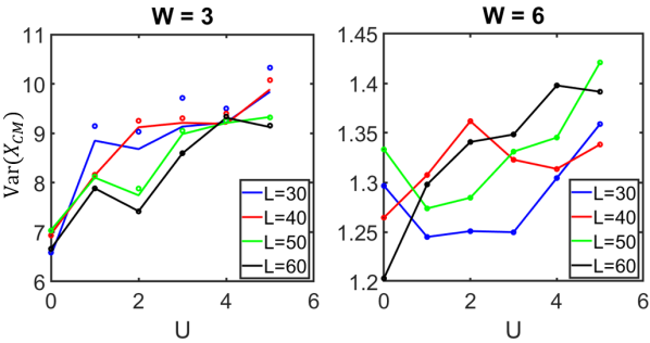
Figure 6: Two particle center of mass variance (solid line) and MBQM (points) versus interaction strength. Left we plot the results for a disorder strength of $W=3$ where for smaller systems the two quantities do not agree well, but become closer as the system size increases. Right depicts the same quantities at disorder of $W=6$. For this larger disorder all system sizes show agreement between the variance and the MBQM.

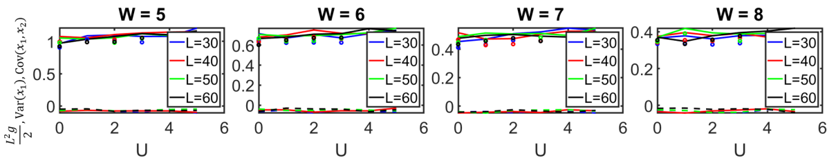
Figure 7: Two particle variance (solid line), covariance (dashed line) and MBQM per particle (points). Colors correspond to system lengths as shown on the figure. Note that the covariance is nearly zero compared with the variance and that the MBQM and the variance agree very well.

III Density Profiles

We provide density profiles of the zero energy eigenstate for a realization of the half-filled disordered hardcore Bose-Hubbard model in Fig. 8. For these density profiles we have fixed the interaction strength to $U=5$. The profiles provided correspond to disorder strengths $W=2,4,6,$ and $8$. Note that there is a qualitative difference between the density profiles when the disorder increases and the wave function becomes less uniform as the system enters the MBL phase. Further note that while this qualitative change occurs, the density is nonzero everywhere in both phases.

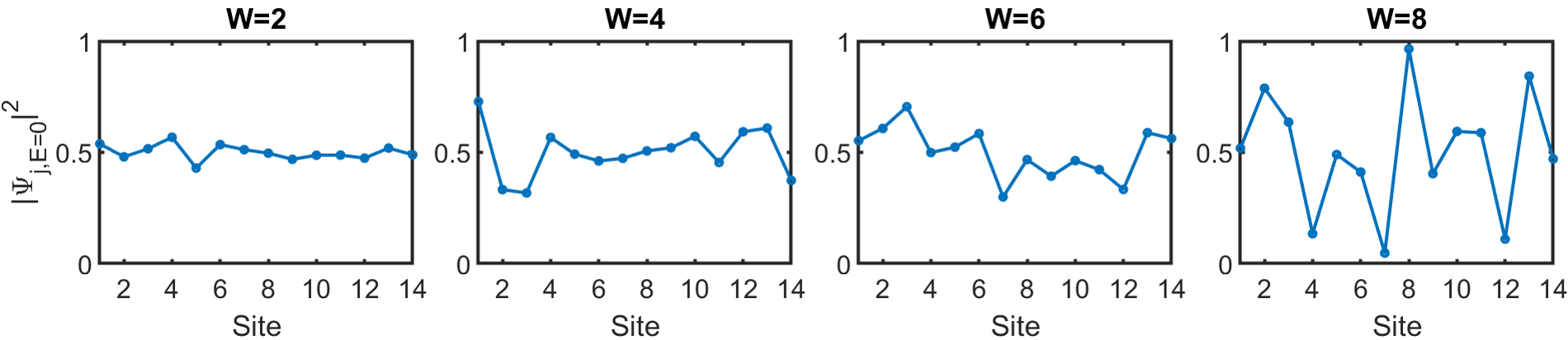
Figure 8: Density profiles of the zero energy eigenstate of the disordered hardcore Bose-Hubbard model. The interaction strength is fixed at $U=5$ and the disorder is varied from 2 to 8 as labelled.

III.1 Additional Detail for Phase Diagram Construction

In this section we present additional results that further support our phase diagram presented in the main text. Firstly, we present our results for the MBQM and the localization length for all disorder strengths considered for completeness in Fig. 9 and in Fig. 10. From these plots it is clear that there is a change in behavior of the MBQM scaling and in the degree of localization as one crosses the phase boundary proposed above.

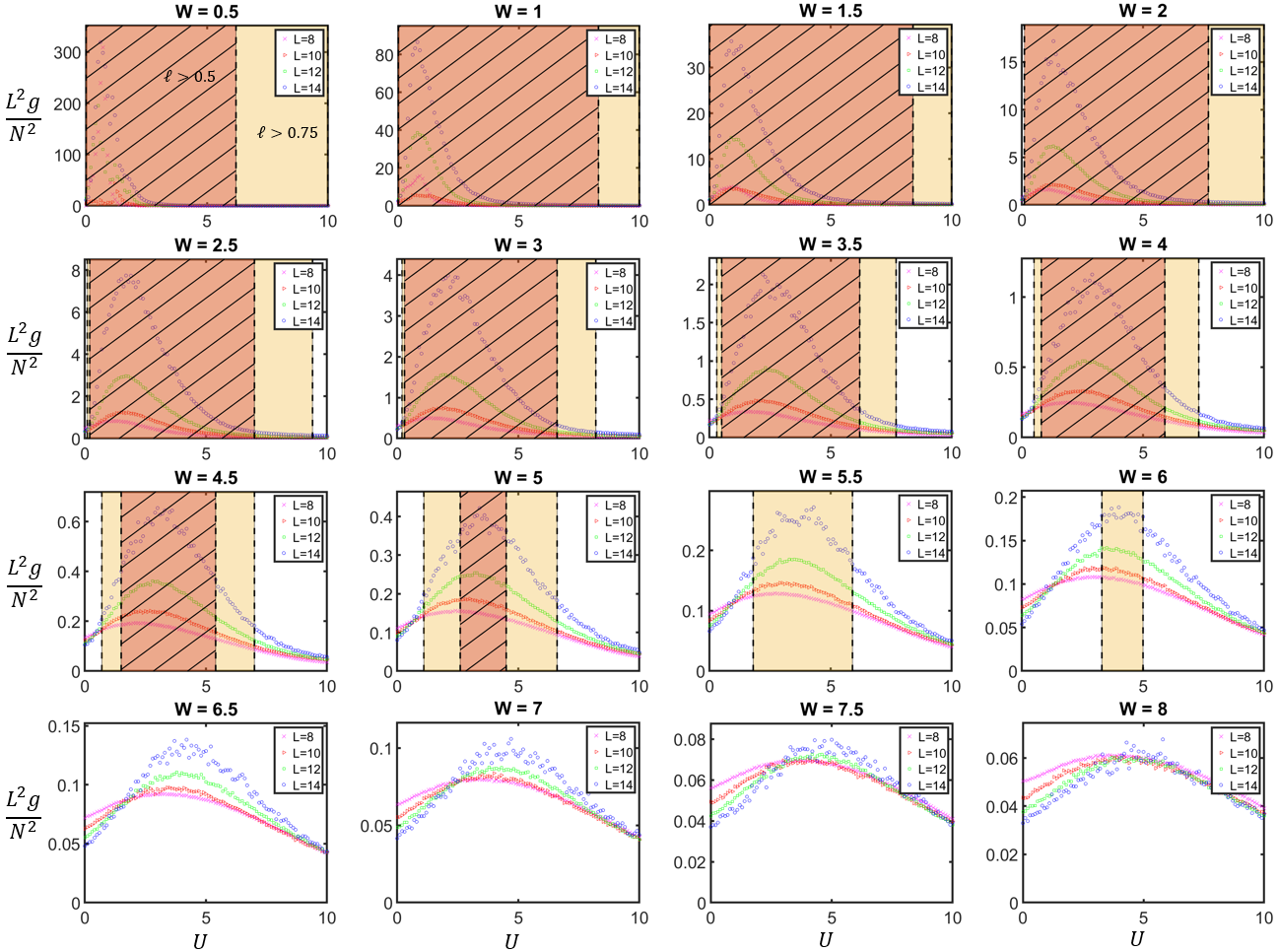
Figure 9: Median MBQM ($L^{2}g/N^{2}$) vs interaction strength for different disorder strengths for different system sizes. The shadings correspond to the ergodic phases, which we define as the region where the quantity $\ell=\lim_{N\to\infty}L\sqrt{g}/N$ is greater than some proposed cutoff. Here the red hatched region corresponds to $\ell>0.5$ and the shaded yellow region corresponds to $\ell>0.75$. We identify the unshaded region as MBL phase for both cutoff choices.

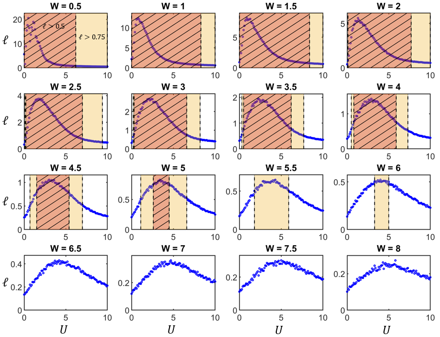
Figure 10: Localization length versus interaction strength for all disorder strengths considered here. The localization length is extracted from the thermodynamic limit as defined in the main text, i.e. $\ell=\lim_{N\to\infty}L\sqrt{g}/N$.

In Fig. 11, we provide further examples of the linear and quadratic fittings in $1/N$ to highlight the subtlety in distinguishing the correct fitting with the few available system sizes. For some parameters, it is clear that a linear fitting is much more accurate than the quadratic fitting. Unfortunately, the preferred fit can be ambiguous for many parameters. This ambiguity can be attributed to the few number of system sizes available and potentially finite size effects. While there is clearly a difference in scaling in different regimes, we find it is best to use a linear fitting across all parameters and compare the corresponding thermodynamic limit to draw our phase boundary.

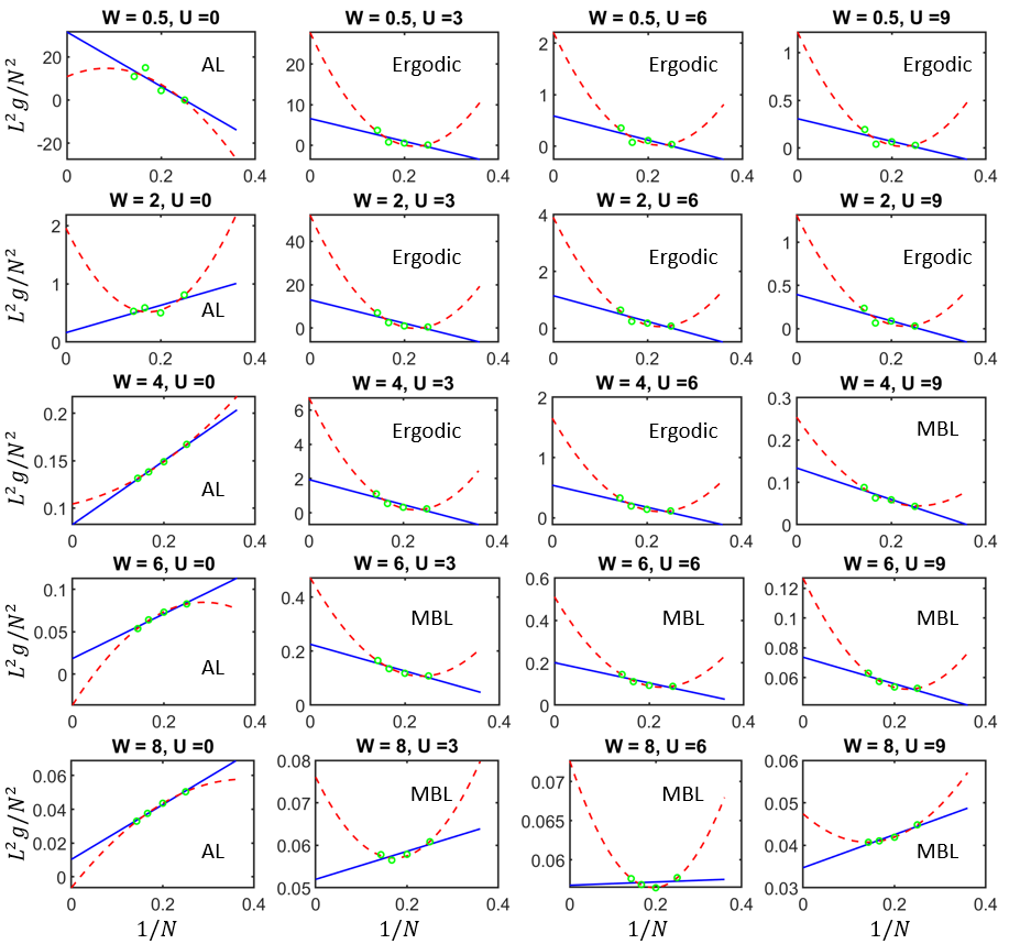
Figure 11: Linear and quadratic fittings of the MBQM for a selection of parameters. We label the predicted phase on each boundary including Anderson localized (AL) for the case of non-interacting systems alongside the MBL and ergodic phases. We set the boundary between MBL and ergodic phases at $\ell=0.5$.

To quantitatively justify our thermodynamic limit, we calculate the least square residuals for the linear fitting, $S_{lin}$, to quantify the goodness of fit at each point in the phase diagram. Here the residuals are defined as

$$S_{lin}=\frac{\sum_{N}(y_{pred,N}-y_{N})^{2}}{\ell^{2}}$$ (6)

where $y_{N}$ is the calculated value of $L^{2}g/N^{2}$ for $N$ particles and $y_{pred,N}$ is the predicted value for $N$ particles from the linear fit. We have normalized the residuals by the thermodynamic limit $\ell^{2}$ to make the comparison between residuals at different parameters meaningful. We plot $\log_{10}S_{lin}$ in Fig. 12. We see that the least square residuals follow precisely the same trend as in Fig. 4 in the main text. We have included contours corresponding to $0.1$, $0.05$, $0.01$, and $0.005$. Note how these contours agree surprisingly well with the contours drawn above based on the localization length.

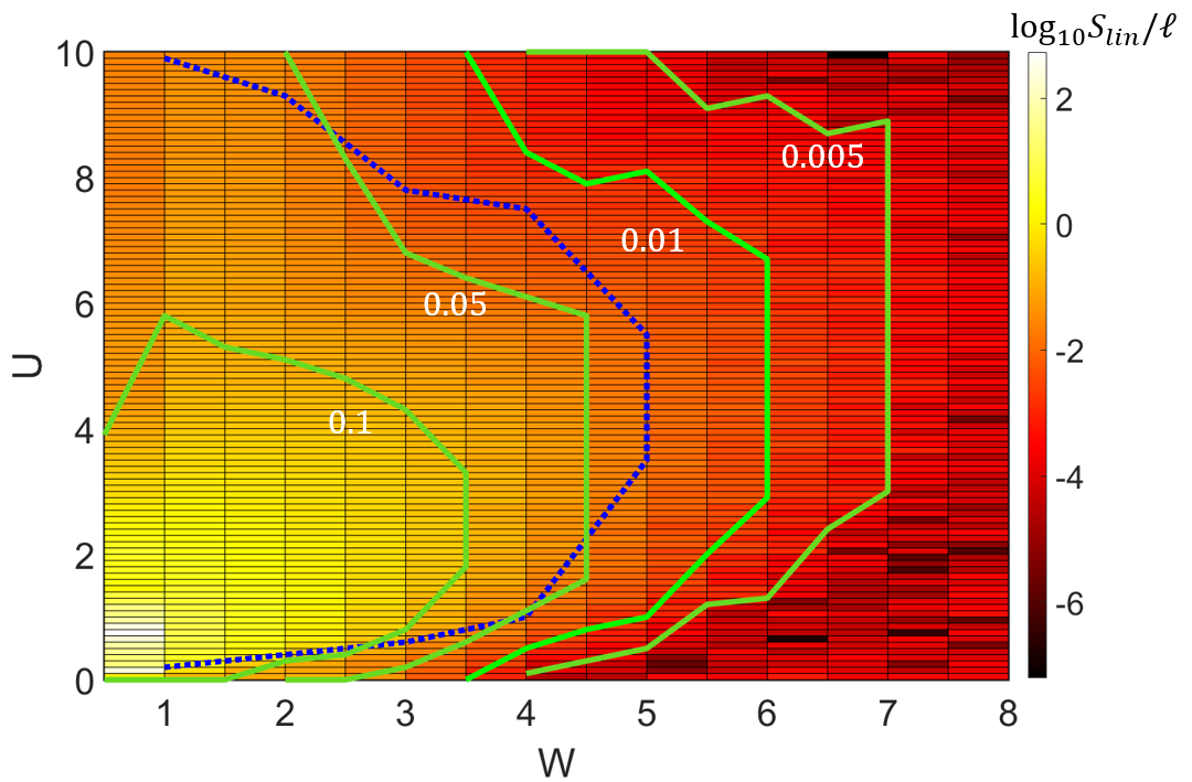
Figure 12: Many Body Localization phase diagram as a function of interaction $U$ and disorder $W$. Color is obtained as $\log_{10}S_{lin}/\ell$. Green curves are labelled with the contour of $0.1$, $0.05$, $0.01$, and $0.005$. The dashed blue contour corresponds to the predicted phase diagram in Ref. [26], demonstrating our method agrees with previously reported investigations.

References

- Bloch et al. [2008] I. Bloch, J. Dalibard, and W. Zwerger, Many-body physics with ultracold gases, Rev. Mod. Phys. 80, 885 (2008).
- Bilokon et al. [2023] V. Bilokon, E. Bilokon, M. C. Bañuls, A. Cichy, and A. Sotnikov, Many-body correlations in one-dimensional optical lattices with alkaline-earth(-like) atoms, Scientific Reports 13, 10.1038/s41598-023-37077-1 (2023).
- Chomaz et al. [2022] L. Chomaz, I. Ferrier-Barbut, F. Ferlaino, B. Laburthe-Tolra, B. L. Lev, and T. Pfau, Dipolar physics: a review of experiments with magnetic quantum gases, Reports on Progress in Physics 86, 026401 (2022).
- Malz and Cirac [2023] D. Malz and J. I. Cirac, Few-body analog quantum simulation with rydberg-dressed atoms in optical lattices, PRX Quantum 4, 020301 (2023).
- Blatt and Roos [2012] R. Blatt and C. F. Roos, Quantum simulations with trapped ions, Nature Physics 8, 10.1038/nphys2252 (2012).
- Adams et al. [2019] C. S. Adams, J. D. Pritchard, and J. P. Shaffer, Rydberg atom quantum technologies, Journal of Physics B: Atomic, Molecular and Optical Physics 53, 012002 (2019).
- Wu et al. [2021] X. Wu, X. Liang, Y. Tian, F. Yang, C. Chen, Y.-C. Liu, M. K. Tey, and L. You, A concise review of rydberg atom based quantum computation and quantum simulation*, Chinese Physics B 30, 020305 (2021).
- Kinoshita et al. [2006] T. Kinoshita, T. Wenger, and D. S. Weiss, A quantum newton’s cradle, Nature 440, 10.1038/nature04693 (2006).
- Vasseur and Moore [2016] R. Vasseur and J. E. Moore, Nonequilibrium quantum dynamics and transport: from integrability to many-body localization, Journal of Statistical Mechanics: Theory and Experiment 2016, 064010 (2016).
- Nandkishore and Huse [2015] R. Nandkishore and D. A. Huse, Many-body localization and thermalization in quantum statistical mechanics, Annual Review of Condensed Matter Physics 6, 15 (2015), https://doi.org/10.1146/annurev-conmatphys-031214-014726 .
- Luca and Scardicchio [2013] A. D. Luca and A. Scardicchio, Ergodicity breaking in a model showing many-body localization, Europhysics Letters 101, 37003 (2013).
- Levi et al. [2016] E. Levi, M. Heyl, I. Lesanovsky, and J. P. Garrahan, Robustness of many-body localization in the presence of dissipation, Phys. Rev. Lett. 116, 237203 (2016).
- Luca D’Alessio and Rigol [2016] A. P. Luca D’Alessio, Yariv Kafri and M. Rigol, From quantum chaos and eigenstate thermalization to statistical mechanics and thermodynamics, Advances in Physics 65, 239 (2016), https://doi.org/10.1080/00018732.2016.1198134 .
- Anderson [1958] P. W. Anderson, Absence of diffusion in certain random lattices, Phys. Rev. 109, 1492 (1958).
- Fleishman and Anderson [1980] L. Fleishman and P. W. Anderson, Interactions and the anderson transition, Phys. Rev. B 21, 2366 (1980).
- Finkel’shtein [1983] A. M. Finkel’shtein, Influence of Coulomb interaction on the properties of disordered metals, Soviet Journal of Experimental and Theoretical Physics 57, 97 (1983).
- Giamarchi and Schulz [1988] T. Giamarchi and H. J. Schulz, Anderson localization and interactions in one-dimensional metals, Phys. Rev. B 37, 325 (1988).
- Altshuler et al. [1997] B. L. Altshuler, Y. Gefen, A. Kamenev, and L. S. Levitov, Quasiparticle lifetime in a finite system: A nonperturbative approach, Phys. Rev. Lett. 78, 2803 (1997).
- Gornyi et al. [2005] I. V. Gornyi, A. D. Mirlin, and D. G. Polyakov, Interacting electrons in disordered wires: Anderson localization and low- transport, Phys. Rev. Lett. 95, 206603 (2005).
- Basko et al. [2006] D. Basko, I. Aleiner, and B. Altshuler, Metal–insulator transition in a weakly interacting many-electron system with localized single-particle states, Annals of Physics 321, 1126 (2006).
- Bauer and Nayak [2013] B. Bauer and C. Nayak, Area laws in a many-body localized state and its implications for topological order, Journal of Statistical Mechanics: Theory and Experiment 2013, P09005 (2013).
- Serbyn et al. [2013a] M. Serbyn, Z. Papić, and D. A. Abanin, Universal slow growth of entanglement in interacting strongly disordered systems, Phys. Rev. Lett. 110, 260601 (2013a).
- Abanin et al. [2019] D. A. Abanin, E. Altman, I. Bloch, and M. Serbyn, Colloquium: Many-body localization, thermalization, and entanglement, Rev. Mod. Phys. 91, 021001 (2019).
- Sierant and Zakrzewski [2018] P. Sierant and J. Zakrzewski, Many-body localization of bosons in optical lattices, New Journal of Physics 20, 043032 (2018).
- Lukin et al. [2019] A. Lukin, M. Rispoli, R. Schittko, M. E. Tai, A. M. Kaufman, S. Choi, V. Khemani, J. Léonard, and M. Greiner, Probing entanglement in a many-body–localized system, Science 364, 256 (2019), https://www.science.org/doi/pdf/10.1126/science.aau0818 .
- Bar Lev et al. [2015] Y. Bar Lev, G. Cohen, and D. R. Reichman, Absence of diffusion in an interacting system of spinless fermions on a one-dimensional disordered lattice, Phys. Rev. Lett. 114, 100601 (2015).
- Schreiber et al. [2015] M. Schreiber, S. S. Hodgman, P. Bordia, H. P. Lüschen, M. H. Fischer, R. Vosk, E. Altman, U. Schneider, and I. Bloch, Observation of many-body localization of interacting fermions in a quasirandom optical lattice, Science 349, 842 (2015), https://www.science.org/doi/pdf/10.1126/science.aaa7432 .
- Bera et al. [2015] S. Bera, H. Schomerus, F. Heidrich-Meisner, and J. H. Bardarson, Many-body localization characterized from a one-particle perspective, Phys. Rev. Lett. 115, 046603 (2015).
- Serbyn et al. [2013b] M. Serbyn, Z. Papić, and D. A. Abanin, Local conservation laws and the structure of the many-body localized states, Phys. Rev. Lett. 111, 127201 (2013b).
- Huse et al. [2014] D. A. Huse, R. Nandkishore, and V. Oganesyan, Phenomenology of fully many-body-localized systems, Phys. Rev. B 90, 174202 (2014).
- Chandran et al. [2015] A. Chandran, I. H. Kim, G. Vidal, and D. A. Abanin, Constructing local integrals of motion in the many-body localized phase, Phys. Rev. B 91, 085425 (2015).
- Rademaker and Ortuño [2016] L. Rademaker and M. Ortuño, Explicit local integrals of motion for the many-body localized state, Phys. Rev. Lett. 116, 010404 (2016).
- Thomson and Schiró [2018] S. J. Thomson and M. Schiró, Time evolution of many-body localized systems with the flow equation approach, Phys. Rev. B 97, 060201 (2018).
- Pekker et al. [2017] D. Pekker, B. K. Clark, V. Oganesyan, and G. Refael, Fixed points of wegner-wilson flows and many-body localization, Phys. Rev. Lett. 119, 075701 (2017).
- Resta [1998] R. Resta, Quantum-mechanical position operator in extended systems, Phys. Rev. Lett. 80, 1800 (1998).
- Resta and Sorella [1999] R. Resta and S. Sorella, Electron localization in the insulating state, Phys. Rev. Lett. 82, 370 (1999).
- Souza et al. [2000] I. Souza, T. Wilkens, and R. M. Martin, Polarization and localization in insulators: Generating function approach, Phys. Rev. B 62, 1666 (2000).
- Resta [2002] R. Resta, Why are insulators insulating and metals conducting?, Journal of Physics: Condensed Matter 14, R625 (2002).
- Lu and Wang [2010] X.-M. Lu and X. Wang, Operator quantum geometric tensor and quantum phase transitions, Europhysics Letters 91, 30003 (2010).
- Valença Ferreira de Aragão et al. [2019] E. Valença Ferreira de Aragão, D. Moreno, S. Battaglia, G. L. Bendazzoli, S. Evangelisti, T. Leininger, N. Suaud, and J. A. Berger, A simple position operator for periodic systems, Phys. Rev. B 99, 205144 (2019).
- Resta [2005] R. Resta, Electron localization in the quantum hall regime, Phys. Rev. Lett. 95, 196805 (2005).
- Wilkens and Martin [2001] T. Wilkens and R. M. Martin, Quantum monte carlo study of the one-dimensional ionic hubbard model, Phys. Rev. B 63, 235108 (2001).
- Thonhauser and Vanderbilt [2006] T. Thonhauser and D. Vanderbilt, Insulator/chern-insulator transition in the haldane model, Phys. Rev. B 74, 235111 (2006).
- Ozawa and Goldman [2019] T. Ozawa and N. Goldman, Probing localization and quantum geometry by spectroscopy, Phys. Rev. Res. 1, 032019 (2019).
- Niu et al. [1985] Q. Niu, D. J. Thouless, and Y.-S. Wu, Quantized hall conductance as a topological invariant, Phys. Rev. B 31, 3372 (1985).
- Banerjee [1996] D. Banerjee, Topological aspects of the berry phase, Fortschritte der Physik/Progress of Physics 44, 323 (1996), https://onlinelibrary.wiley.com/doi/pdf/10.1002/prop.2190440403 .
- Campos Venuti and Zanardi [2007] L. Campos Venuti and P. Zanardi, Quantum critical scaling of the geometric tensors, Phys. Rev. Lett. 99, 095701 (2007).
- Resta [2011] R. Resta, The insulating state of matter: a geometrical theory, The European Physical Journal B 79, 121 (2011).
- Watanabe [2018] H. Watanabe, Insensitivity of bulk properties to the twisted boundary condition, Phys. Rev. B 98, 155137 (2018).
- Kondov et al. [2015] S. S. Kondov, W. R. McGehee, W. Xu, and B. DeMarco, Disorder-induced localization in a strongly correlated atomic hubbard gas, Phys. Rev. Lett. 114, 083002 (2015).
- Note [1] In order to calculate , we first calculate an eigenstate of the Anderson model under the periodic boundary condition, and then calculate the center-of-mass of the wavefunction, which can be done using the framework of Ref. [35]. We then shift the coordinate so that the center of mass is in the middle of the one-dimensional chain, and we calculate taking . Namely, while we calculate the eigenstate under the periodic boundary condition, we calculate assuming the open boundary condition.
- Serbyn et al. [2015] M. Serbyn, Z. Papić, and D. A. Abanin, Criterion for many-body localization-delocalization phase transition, Phys. Rev. X 5, 041047 (2015).
- Mondaini and Rigol [2015] R. Mondaini and M. Rigol, Many-body localization and thermalization in disordered hubbard chains, Phys. Rev. A 92, 041601 (2015).
- Chen et al. [2023] J. Chen, C. Chen, and X. Wang, Many-body localization transition in the disordered bose-hubbard chain (2023), arXiv:2104.08582 [cond-mat.dis-nn] .