The first Ka-band (26.1-35 GHz) blind line survey towards Orion KL

Abstract

We conducted a Ka-band (26.1–35 GHz) line survey towards Orion KL using the TianMa 65-m Radio Telescope (TMRT). It is the first blind line survey in the Ka band, and achieves a sensitivity of mK level (1–3 mK at a spectral resolution of $\sim$1 km s^-1). In total, 592 Gaussian features are extracted. Among them, 257 radio recombination lines (RRLs) are identified. The maximum $\Delta n$ of RRLs of H, He and C are 20, 15, and 5, respectively. Through stacking, we have detected the $\beta$ lines of ion RRLs (RRLs of C⁺ with possible contribution of other ions like O⁺) for the first time, and tentative signal of the $\gamma$ lines of ion RRLs can also be seen on the stacked spectrum. Besides, 318 other line features were assigned to 37 molecular species, and ten of these species were not detected in the Q-band survey of TMRT. The vibrationally excited states of nine species were also detected. Emission of most species can be modeled under LTE. A number of transitions of E-CH3OH ($J_{2}-J_{1}$) display maser effects, which are confirmed by our modeling, and besides the bumping peak at $J\sim 6$ there is another peak at $J\sim 13$. Methylcyanoacetylene (CH₃C₃N) is detected in Orion KL for the first time. This work emphasizes that the Ka band, which was long-ignored for spectral line surveys, is very useful for surveying RRLs and molecular lines simultaneously.

1 Introduction

Table 1: The line surveys of Orion KL in low frequency range ($\nu<50$ GHz).

Frequency coverage(1)	Telescope	Spectral resolution	Sensitivity(2)	Reference(4)
17.9–26.2 GHz	Effelsberg 100 m	61 kHz ($\sim$0.7 km s-1)	5–22 mK	Gong et al. (2015)
26.1–35 GHz	TMRT 65 m	92 kHz ($\sim$0.9 km s-1)	1–3 mK	This work
34.8–50 GHz	TMRT 65 m	92 KHz ($\sim$0.65 km s-1)	1.5–5 mK(3)	Liu et al. (2022)
41.5–50 GHz	DSS-54 34 m	180 kHz ($\sim$1.2 km s-1)	8–12 mK	Rizzo et al. (2017)

⁽¹⁾ Only wide-band blind line surveys are listed here.
⁽²⁾ The line sensitivity in $T_{\rm MB}$ scale at the corresponding spectral resolution.
⁽³⁾ The line sensitivity at 49–50 GHz is slightly worse with a value of 5–8 mK.
⁽⁴⁾ Little can be known about the line survey of Ohishi et al. (1986) from its relevant published work. From the spectra of all of its covered frequency bands (34.25–50, 83.5–84.5, and 86–91.5 GHz), Ohishi et al. (1986) detected 19 molecular species, much smaller than the values of 39 and 53 detected in Q band alone by Rizzo et al. (2017) and Liu et al. (2022).

The low-frequency ($<$50 GHz) line surveys have advantages in searching for complex organic molecules (COMs) and radio recombination lines (RRLs), because low-frequency lines tend to be non-seriously blended and more easily excited compared with those in higher frequency ranges. In contrast to the ample surveys at the high-frequency millimeter and submillimeter bands ($\nu>70$ GHz; e.g., Johansson et al., 1984; Turner, 1989; Schilke et al., 1997, 2001; White et al., 2003; Tercero et al., 2010), there are only a scarcity of line surveys at low-frequency bands towards Orion KL (e.g. Corby et al., 2015; Gong et al., 2015; Rizzo et al., 2017), which is the nearest ($\sim$414 pc; Menten et al., 2007) high-mass star forming region and one of the most representative objects of line surveys. The emission of Orion KL is complex (e.g., Tercero et al., 2010), with contributions from several physical components including the foreground Hii region M42 (Wilson et al., 1997), the PDR between M42 and the molecular cloud (e.g., Natta et al., 1994), the externally heated “compact ridge” (e.g., Mangum & Wootten, 1993; Wang et al., 2011; Tahani et al., 2016), the hot cores (e.g., Mangum & Wootten, 1993; Jacob et al., 2021), the extended ridge and plateau (e.g., Genzel & Stutzki, 1989; Bernal et al., 2021) as well as some other millimeter continuum sources (e.g., Wu et al., 2014). It makes Orion KL rich in spectral lines at different frequency bands (e.g., Blake et al., 1987; Schilke et al., 1997; Tercero et al., 2010; Crockett et al., 2014; Rizzo et al., 2017). This motivated us to conduct a multi-band low-frequency line survey using the Tianma 65-m Radio Telescope (TMRT) towards Orion KL (referred as the TMRT line survey below), aiming to obtain an unprecedented sensitive template for low-frequency spectra (with a line sensitivity of one or several mK), covering the whole working frequency range (1–50 GHz) of the TMRT.

The ongoing TMRT line survey began with the Q-band (35-50 GHz) pioneer survey (Liu et al., 2022), which is so far the most sensitive one compared with previous wide-band Q-band surveys of Orion KL (Ohishi et al., 1986; Rizzo et al., 2017). It reached a sensitivity at a level of 1.5-5 mK (Table 1) and 597 Gaussian features were extracted, proving the capability for the TMRT of conducting deep line surveys. In the Q band, the number of detected molecular lines, 395, is more than twice the number of RRLs, 153. Most of the Q-band molecular lines are emission of complex organic molecules (COMs). In contrast, the K-band (18–26 GHz) spectrum of Orion KL was found to be dominated by RRLs, as revealed by the survey of Gong et al. (2015) that have identified 164 RRLs among the 261 detected lines. It is reasonable to expect that the Ka-band (26–35 GHz) spectrum of Orion KL would have comparable numbers of RRLs and molecular lines, making the Ka band very suitable for observing COMs and RRLs simultaneously.

Despite its promising potential uses, the Ka band was long-ignored for spectral line surveys, and acted as a frequency gap especially for single-dish observations. This frequency range is usually preferred for satellite communication (e.g., Vanelli-Coralli et al., 2015), and was historically avoided for radio astronomy. It makes the Ka band a missing piece for previous line surveys (Table 1). To fill in this blank gap, we conducted a Ka-band (26–35 GHz) survey of Orion KL as a part of the TMRT line survey, following the Q-band one (Liu et al., 2022). Through long-time integrations, a line sensitivity of 1–3 mK was achieved with a frequency resolution of 91.553 kHz. This is the first blind line survey in the Ka band reaching a line sensitivity of mK level.

In Liu et al. (2023), we have reported the successful detection of the ion RRLs (X⁺ RRLs with X⁺ referred to C and/or O) in the interstellar medium for the first time, through combining the data of the TMRT surveys in three bands (Ka, Ku, and Q). This Ka-band survey is the most sensitive one, compared with the less sensitive Q-band survey and the partly executed Ku-band survey. It expanded the scope of our understanding of ion RRLs, because prior to that work, only two blended lines (105$\alpha$ and 121$\alpha$) of He II in planetary nebulae had been reported (Chaisson & Malkan, 1976; Terzian, 1980; Vallee et al., 1990).

In this work, we present the overall results of the Ka-band (26.1–35 GHz) line survey of Orion KL. The paper is structured as follows: In Section 2 we introduce the observations. In Section 3 we describe the procedures of data reduction, line identification and emission modeling of RRLs and molecular lines. In Sections 4 and 5, we present more detailed results about the RRLs and molecular lines, respectively. We provide a summary in Section 6.

Figure 1: The overview of the Ka-band (26.1–35 GHz) spectrum of Orion KL observed by the TMRT. Lower panel: A zoomed-in view of the same spectrum. (The data used to create this figure are available online.)

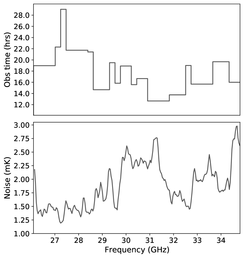
Figure 2: The observation time (upper) and rms noise (lower) of the Ka-band spectrum. Both the on-source and off-source integration time have been included to calculate the observation time.

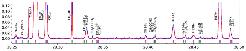
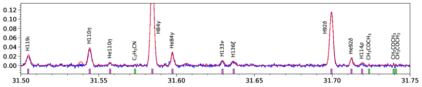
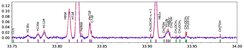
Figure 3: The images of Ka-band spectrum of Orion KL. The x-axis is rest frequency in units of gigahertz (with a Doppler correction applied adopting a $V_{\rm LSR}$ of 6 km s^-1). The $y$-axis is $T_{\rm MB}$ in units of kelvin. The blue line is the Orion KL spectrum observed by the TMRT 65 m, which has been smoothed to have a frequency resolution of 183 kHz ($\sim$1.8 km s^-1 at 30 GHz). The red line represents the modeling fitting. The purple strips denote the detected RRLs. The green strips denote the molecular lines. The gray strips mark the U lines. See Figure 16 for all the spectral images.

2 Observations

2.1 Ka-band receiving system of TMRT

The observations were carried out using the TMRT, built and operated by the Shanghai Astronomical Observatory. The TMRT is located in the western suburb of Shanghai, China. It has an aperture diameter of 65 m, corresponding to a full-width at half-maximum (FWHM) of the primary beam of $\sim$46″–34″ at 26–35 GHz. Its Ka receiver is a two-beam dual-polarization (LCP and RCP) cryogenic receiver, covering 26–40 GHz, with the 35–40 GHz overlapping with the working frequency range of the Q-band receiver. The beam 2 was employed for our single-pointing observations. The receiver noise temperatures were 10-30 K, and the system temperatures ($T_{\rm sys}$) ranged from 60 K to 150 K, depending on the frequency, elevation and especially the weather conditions (Wang et al., 2017b).

During the preparation for this survey, the Ka-band pointing model of the TMRT was updated through tracking strong continuum sources, including DR21 and 3C84, for one whole day, following the method of Wang et al. (2017a). The pointing accuracy was better than 5 arcsec. The aperture efficiency is nearly constant (0.5$\pm$0.1) thanks to the active surface control utilizing actuators which can compensate for the gravity deformation of the main reflector during observations (Dong et al., 2018). For calibration, the signal of noise diodes was injected lasting for one second within each two-second period. In summer, the high water vapour content and deformation by sunlight make TMRT difficult to be used for Ka/Q-band observations. Under typical weather conditions at the TMRT in the winter semester, the zenith atmospheric opacities were 0.1 in the Ka band (Wang et al., 2017b). Calibration uncertainties were estimated to be within 20%.

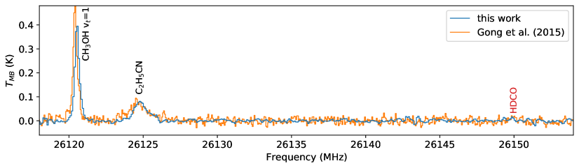
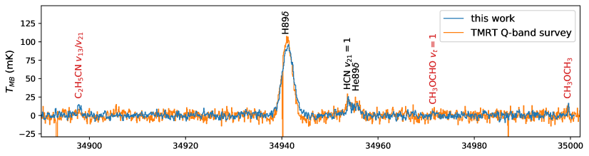
Figure 4: Upper: Comparison between the spectra of this Ka-band (26.1–35 GHz) survey and of the K-band (17.9–26.2 GHz) survey of Effelsberg 100 m by Gong et al. (2015). See Section 3.1 for possible reasons of the slight velocity discrepancy (by about two channels) between the two surveys. Lower: Comparison between the spectra of this Ka-band survey and the TMRT Q-band (34.8–50 GHz) survey (Liu et al., 2022). The overlapping frequency ranges of those surveys are located at the edges of the frequency coverages, and consequently have relatively poor sensitiveties. Note that the lower panel has has wider frequency range than that of the upper panel.

2.2 The Ka-band survey

This Ka-band line survey of Orion KL covered 26.1–35 GHz. Although the working frequency range of the K-band receiver is 26–40 GHz, the 35–40 GHz was not covered by this survey, because it has been done by our previous Q-band line survey (Liu et al., 2022). The 26–26.1 GHz was not covered because of the limitation of the bandpass filter. The digital backend system (DIBAS) of TMRT is an FPGA-based spectrometer based on the design of the Versatile GBT Astronomical Spectrometer (Bussa & VEGAS Development Team, 2012), and it provides 29 observing modes. The setup of the backend for the Ka-band survey is the same as that of the Q-band survey (Liu et al., 2022). Two banks (the third one is not available at present) have a bandwidth of 1.5 GHz each, and they work independently with no limitation on the separation between their central frequencies. Under the mode 2 of DIBAS, each polarization of each bank has 16384 channels, and the channel width is 91.553 kHz, corresponding to a velocity resolution ($\delta V$) of $\sim$0.92 km s^-1 at 30 GHz.

The observations were conducted from September 28th to October 30th, 2022. The targeting position is RA(J2000)=05:35:14.55, DEC(J2000)=$-$05:22:31.0. Different physical components of Orion KL (see Section 1) can be covered by a single beam of the TMRT, as depicted in our previous Q-band survey (Liu et al., 2022). Position-switching observation mode was adopted, with the off points 15′ away (in azimuth direction) from the target. The offset value is much larger than 4′, the angular size of the brightest region of M42 (Yusef-Zadeh, 1990; Wilson et al., 1997). We periodically integrated two minutes in each position (on/off). During observations of this survey, pointing was checked every two hours.

For each frequency bank, its frequency coverage in the sky frequency scale was fixed. The frequency of the local oscillator (LO) did not change during the observation for a single frequency setup. The spectrum of each on-off repeat was corrected from the topocentric frame to the frame of the local standard of rest (LSR) during data processing. The frequencies of the two banks were shifted in different setups to cover 26.1–35 GHz. For most frequency ranges of Ka band, there is no noticeable radio frequency interference (RFI) on the spectrum. At some narrow frequency ranges (e.g., $\sim 26.4-26.8$ GHz), RFI can be sometimes very strong but it does not last for a long time. Each frequency point was covered by at least two different frequency setups observed on different days. The spectra with obvious RFI were manually dropped. Each of the observed frequency points is covered by a telescope time of 12–25 hours, depending on the weather conditions.

3 Observational results

3.1 Data reduction

The spectra of each polarization of each frequency were first averaged weighted by $1/T_{\rm sys}^{2}$. The averaged spectrum was then chopped into segments of 100 MHz. For each segment, we manually fit the spectral baseline and get the noise of each segment using the procedure provided by Gildas/CLASS (Guilloteau & Lucas, 2000). To conduct this procedure, the frequency intervals that contain visible line features or spectral emission predicted from the Q-band data (Liu et al., 2022) have been masked out. We further converted the frequency of the spectrum from the LSR frame to the rest frame of Orion KL assuming a systematic velocity of Orion KL ($V_{\rm LSR}$) of 6 km s^-1. Finally, we spliced together all the segments weighted by their noise levels to obtain the final Ka-band spectrum, covering 26.1–35 GHz with a frequency resolution of 91 kHz.

The final spectrum (in $T_{\rm MB}$ scale) is shown in Figure 1. To estimate the rms noise of the spectrum, we first masked out all the extracted emission features and bad channels (Sect. 3.2), and then for each channel we calculated the standard deviation of the intensities of its unmasked neighbour channels within 25 MHz. As expected, the rms noise is roughly inversely proportional to the integration time. The 26.1–26.2 GHz is close to the edge of the working frequency of the TMRT in the Ka band, and can not be placed in the inner region of a frequency bank which has better performance. Thus, the noise level of 26.1–26.2 GHz is slightly higher (Figure 2). The rms noise of the final spectrum ranges from 1 mK to 3 mK, with a mean value of 1.87 mK and a median value of 1.80 mK.

Table 2: The number of RRLs and molecular lines detected by different surveys⁽¹⁾.

Ref.	$N_{l}$	$\rho_{l}$	$N_{\rm RRL}^{(2)}$	$N_{\rm mol}^{(3)}$	$N_{RRL}^{\rm mol}$	$N_{\rm U}$	$N_{\rm RRL}$/$N_{\rm mol}^{(4)}$
This work	592	64	257(12)	318(20)	7	10	0.9
Liu et al. (2022)	596	36	153(13)	395(50)	9	39	0.6
Rizzo et al. (2017)	227	26	66	143	–	18	0.5
Gong et al. (2015)	261	32	164	97	–	–	1.7

⁽¹⁾ $N_{l}$ is the total number of detected line features. $\rho_{l}$ is the averaged number of detected line features per GHz. $N_{\rm RRL}$ is the number of RRLs, including those blended with other RRLs. $N_{\rm mol}$ is the number of molecular lines, including those blended with other molecular lines. $N_{\rm RRL}^{\rm mol}$ is the number of line features blended by both RRLs and molecular emission. $N_{\rm U}$ is the number of U lines.
⁽²⁾ The values in the brackets represent the number of line features blended by more than one RRL but no molecular transition.
⁽³⁾ The values in the brackets represent the number of repeated molecular line features because of multiple velocity components.
⁽⁴⁾ The ratio between the number of detected transitions of RRLs and molecular transitions.

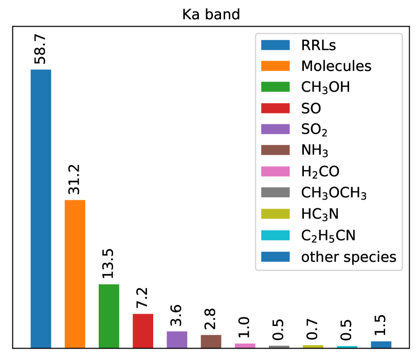
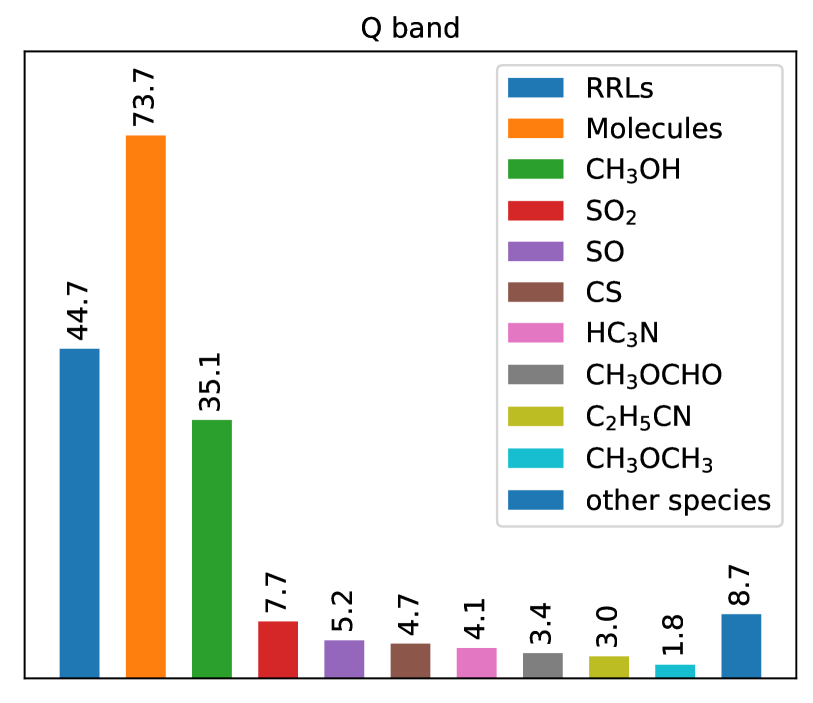
Figure 5: The total Ka-band (upper) and Q-band (lower) emission flux (in units of K MHz) of detected species.

Figure 3 shows examples of the zoom-in Ka-band spectrum. The lower end of the Ka-band spectrum (26.1–26.16 GHz) was also covered by the K-band survey of the Effelsberg 100 m telescope (Gong et al., 2015). The upper end of the Ka-band spectrum (34.88–50 GHz) was also covered by the Q-band survey of the TMRT (Liu et al., 2022). Figure 4 compares the overlapped spectra of the three surveys. Note that the transition of CH₃OH at $\sim$26120 MHz on the K-band spectrum is slightly redder (by two channels) than that on the Ka-band spectrum. This may be caused by the slightly different targeting centers of the two surveys. The target of the K-band survey is located at 16″ south-west of the target of this survey, which is smaller than the beam sizes of both the TMRT and the Effelsberg 100 m. The intersection between the fields of view of the two surveys covers more than half the primary beam of the TMRT (see Figure 1 of Liu et al. (2022)). We modeled the K-band spectral emission based on the Ka band spectra, and compared the observed and modeled spectra of RRLs and CH₃OH in the K band. The K-band spectra around 26 GHz are all redshifted by about two channels compared with the model. However, this is not a systematical trend in the whole K band since in some frequency ranges the velocities match each other. The velocities of the Q-band spectra of RRLs and CH₃OH by by Liu et al. (2022) and Rizzo et al. (2017) were consistent with each other, as highlighted by the Figure 5 of Liu et al. (2022). The velocities of the Ka-band RRLs are self-consistent and are consistent with the modeled spectrum derived based on Q-band emission parameters (Liu et al., 2022). Therefore there is no systematical frequency bias in the Ka-band survey. The small velocity discrepancy between this survey and the K-band survey (Gong et al., 2015) has no influence on the comparison between the two surveys.

Among the three surveys, the Ka-band survey has the best sensitivity (Table 1), and can detect emission lines that have not been detected by the previous Q-band and K-band surveys, although the overlapped frequency ranges are very narrow. The main-beam temperatures of spectral lines from extended regions (e.g., RRLs) measured by different surveys should be consistent with each other. The aperture of Effelsberg is larger than that of the TMRT. Thus, for spectral lines originate from more compact regions, e.g., the transition of CH₃OH $v_{t}=1$ at 26120.6 MHz, their main-beam temperatures measured by the TMRT are slightly lower than that by the Effelsberg as expected due to potentially smaller filling factors (see the upper panel of Figure 4).

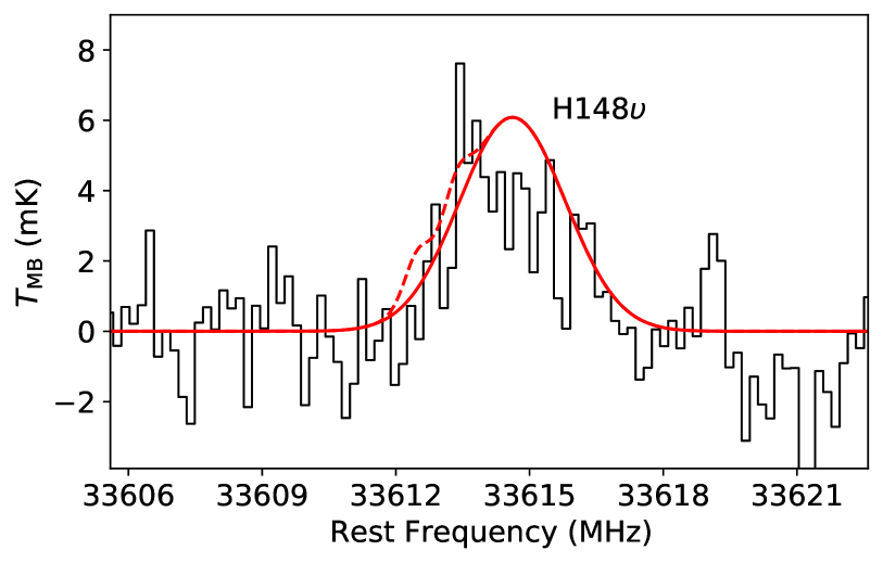
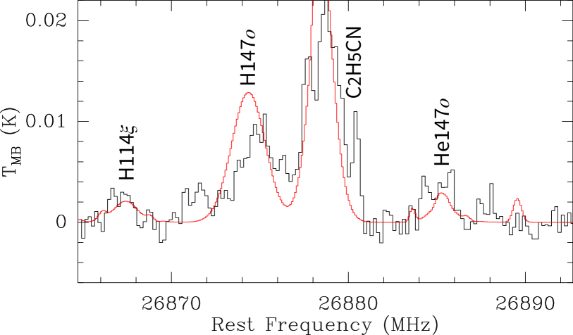
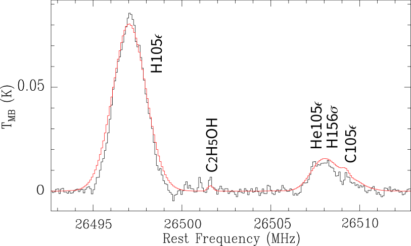
Figure 6: Example of the detected RRLs with large $\Delta n$. The red lines represent the result of model fitting of RRLs and molecular lines. The dashed line in the upper panel has taken into account the emission of C₂H₅CN $\varv_{13}$/$\varv_{21}$.

3.2 Line identification

We visually searched for line features on the Ka-band spectrum. Then, Gaussian fittings were manually conducted to those possible line features one by one using the fitting procedure provided by the GILDAS/CLASS. For blended lines or strong lines with obvious non-Gaussian shapes, multiple Gaussian fittings were applied. In total, 592 Gaussian components (referred to line features) were extracted (Tables 2, 6, and 7).

Then, we modeled the Ka-band spectrum based on the physical parameters fitted from the Q-band observations following Liu et al. (2022). Most of the Ka-band line features can be reproduced by the physical parameters of species detected in the Q band. We first coarsely crossmatched those line features with RRLs of H, He and C, and the transitions of molecules detected in the Q-band survey. Further, we tried to assign the unmatched lines to species undetected in the Q-band survey. A species was marked as detected when more than one of its transitions were detected above 3$\sigma$ and can be reproduced by the emission model with parameters compatible with values in the literatures (e.g., Tercero et al., 2011; Gong et al., 2015; Rizzo et al., 2017; Liu et al., 2023). The species with only one line feature in the Ka band is also marked as detected if it is detected in the Q band. For vibrationally excited species, it would be marked as detected even if only one of its rotational lines is detected, as long as that transition is consistent with the model prediction based on the physical parameters of its corresponding ground-state species (e.g., E-CH₃OH $v_{t}=1$ in Section 5.1). See Sections 4 and 5 for the details about the model fitting process of RRLs and molecular lines, respectively. We iterated the above procedures trying to properly assign as many as possible detected line features. Finally, the still unmatched line features are marked as unidentified lines (marked as ‘U’).

Table 6 lists the molecular lines and unidentified lines, including those blended with RRLs. Table 7 lists the RRLs which are not blended with any molecular emission.

Table 3: The maximum $\Delta n$ of RRLs detected in Orion KL.

Ref.	band	frequency	H	He	C	X+
This work	Ka	26.1–35 GHz	20	15	5	2,3(1)
Liu et al. (2022)	Q	35–50 GHz	16	7	3	–
Liu et al. (2023)	Ku/Ka/Q	12–18 GHz, 26.1–50 GHz	–	–	–	1
Rizzo et al. (2017)	Q	41.5–50 GHz	11	4	2	–
Gong et al. (2015)	K	17.9–26.2 GHz	11	4	1	–
Bell et al. (2011)	C	5.98–6.05 GHz	21,25(2)	6	–	–

⁽¹⁾ Through stacking (Section 4.3). The signal of the stacked $\gamma$ ($\Delta n=3$) is marginal, and the stacked $\beta$ ($\Delta n=2$) line is more reliable (Section 4.3).
⁽²⁾ An H RRL with $\Delta n$ of 25 was reported but only has an intensity of 2$\sigma$. Note that the H RRL with $\Delta n=21$ (H274$\phi$ at 6013.5 MHz) detected by Bell et al. (2011) is close to He230$\mu$ (6013.8 MHz). Although, under LTE, the intensity of He230$\mu$ is only one fourth the value of H274$\phi$.

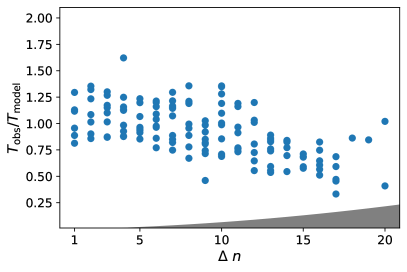
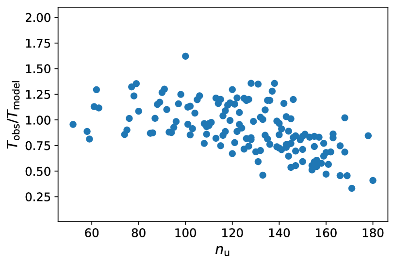
Figure 7: Upper: The correlation between $\Delta n$ and the intensity ratio between observation and model ($T_{\rm obs}/T_{\rm model}$). The gray area represents the 1-$\sigma$ uncertainty of $T_{\rm obs}/T_{\rm model}$. Only the uncertainty of spectral noise is considered here, and the uncertainty contributed by calibration is not taken into account. Lower: The correlation between upper-level principle quantum number ($n_{\rm u}$) and $T_{\rm obs}/T_{\rm model}$. The two panels are only for H RRLs.

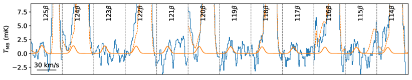
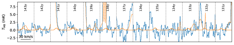
Figure 8: The Ka-band X${}^{+}n\beta$ (upper panel) and X${}^{+}n\gamma$ (lower panel) lines of ion RRLs (blue lines). The orange lines are the modeled spectrum. The orange dashed line takes emission of all species (molecular transitions and RRLs) into account, and the orange solid line only considers the ion RRLs. We note that, these X${}^{+}n\beta$ and X${}^{+}n\gamma$ RRLs were not detected individually, and some of them were at most marginally detected. See Figure 9 for the stacked spectra.

3.3 Overview of the spectral lines

Although the bandwidth of this Ka-band line survey ($\sim$9 GHz) is narrower than that of the Q-band survey of the TMRT (15 GHz), the number of line features detected by the two surveys are comparable, partly because the Ka-band survey has a higher sensitivity and the weak line features can be detected (Table 1). The line density ($\rho_{l}$), defined as the averaged number of line features detected per GHz, of this survey is nearly twice the $\rho_{l}$ of previous surveys in the K and Q bands (Table 2). The Q-band spectrum of Orion KL is dominated by molecular transitions (Rizzo et al., 2017; Liu et al., 2022), and the ratio between the numbers of RRLs and molecular transitions, 0.5, is weakly dependent on the sensitivity (Table 2). In contrast, the K-band spectrum is dominated by RRLs (Gong et al., 2015). Among the 592 line features of this survey, the number of transitions of RRLs, 263, and molecular transitions, 305, are comparable with each other. The total emission flux contributed by RRLs, 58.7 K MHz, is also comparable with that by molecular transitions, 35.2 K MHz (Figure 5). Thus, the Ka band, a long-ignored window for spectral line surveys located between the K band and Q band, is very useful for studying RRLs and molecular lines simultaneously.

The U lines are all weak ($T_{\rm peak}<10$ mK) and some of them are narrow spikes (Table 6 and Figure 3). The Ka-band survey is deeper than the Q-band survey, and we have dropped the data of bad quality during the observations since there were usually several different frequency setups for each frequency range (Section 2.2). This is why the Ka-band survey has much less spikes and bad channels than in the Q band (Table 2).

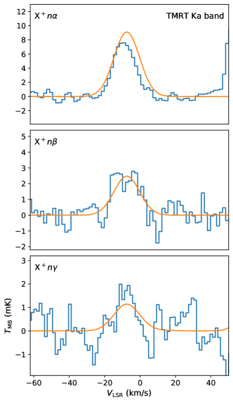
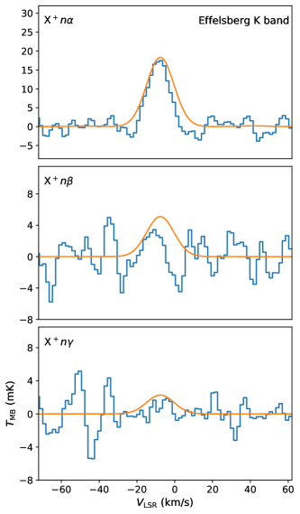
Figure 9: The blue lines are the $\alpha$ (top), $\beta$ (middle) and $\gamma$ (bottom) lines of ion RRLs stacked from the spectra of Orion KL measured in Ka band using the TMRT 65 m (left) and in K band using the Effelsberg 100 m by Gong et al. (2015) (right). The orange lines are the modeled spectra of ion RRLs. The orange lines in the right panels have been multiplied by a factor of 0.8. Only the unblended transitions are stacked. Specifically, in Ka band, we stacked ${\rm X}^{+}n\alpha$ ($n=$ 99, 97, 95, 92, 91), ${\rm X}^{+}n\beta$ ($n=$ 123, 121, 119, 117, 115) and ${\rm X}^{+}n\gamma$ ($n=$ 142, 137, 136, 134, 131). In K band, we stacked ${\rm X}^{+}n\alpha$ ($n=$ 112, 111, 110, 108, 107, 106, 105, 104, 103, 101, 100), ${\rm X}^{+}n\beta$ ($n=$ 141, 137, 135, 131, 127) and ${\rm X}^{+}n\gamma$ ($n=$ 162, 159, 158, 156, 153, 148, 147, 146, 145, 144).

4 RRLs

The rest frequencies of RRLs can be calculated from the Rydberg formula (e.g., Towle et al., 1996; Gordon & Sorochenko, 2002)

$$\nu^{\rm RRL}_{\rm rest}(n+\Delta n,n)=\frac{m_{e}^{\prime}}{m_{e}}R_{\infty}cZ^{2}\left(\frac{1}{n^{2}}-\frac{1}{(n+\Delta n)^{2}}\right)$$ (1)

with

$$m_{e}^{\prime}=\frac{M-Zm_{e}}{M-(Z-1)m_{e}}.$$ (2)

Here, $M$ and $Z-1$ are the total mass and atomic charge of a hydrogenic emitter, respectively, $m_{e}$ is the electron mass, $m_{e}^{\prime}$ is the reduced mass of the electron, and $R_{\infty}=109737.31568$ cm^-1 (Tiesinga et al., 2021). The value of $n$ is large for RRLs and it is thus valid to treat the emitters as hydrogenic. For RRLs of neutral atoms recombined from singly ionized ions ($X^{+}$ or X II), $Z$ should be adopted as one. For RRLs of singly ionized ions recombined from doubly ionized ions ($X^{2+}$ or X III), Z should be adopted as two. In this work, the RRLs with $Z=1$ and $Z>1$ are refereed as neutral RRLs and ion RRLs, respectively.

In total, 257 emission features in this survey are assigned to RRLs, including 245 unblended ones (Tables 2, 6, and 7). The RRLs contribute to 60 percent of the total emission flux of the spectral lines in Ka band (Figure 5). In Liu et al. (2023), we have reported the first detection of the $\alpha$ lines of RRLs of carbon and/or oxygen ions in the interstellar medium. In below sections, we would display all the RRLs detected in the Ka band towards Orion KL (Section 4.1), including the high-order neutral RRLs with the maximum value of $\Delta n$ reaching 20 (Section 4.2), reported the first detection of ion RRLs with $\Delta n>1$ (the $\beta$ and $\gamma$ lines) through stacking all the unblended transitions (Section 4.3).

Table 4: Model parameters of molecules ⁽¹⁾

Species	size(2)	$T_{\rm ex}$	$N_{\rm tot}^{(3)}$	$\Delta V$	$V_{\rm lsr}$
	(″)	(K)	(cm-2)	(km s-1)	(km s-1)
H2CS	20	100	1.8e+15	4.0	8.0
CCS	30	100	1.2e+13	8.0	7.5
SO	15	100	1.2e+17	15.0	6.0
	15	100	2.2e+17	25.0	9.0
34SO	15	100	4.8e+15	15.0	6.0
	15	100	9.6e+15	25.0	9.0
SO2	40	50	5.0e+15	4.0	7.0
	40	200	6.0e+15	10.0	7.0
	40	100	1.9e+16	25.0	7.5
34SO2	40	50	1.0e+14	4.0	7.0
	40	200	6.0e+14	10.0	7.0
	40	100	6.0e+14	25.0	7.5
HCN $\varv_{2}=1$	15	200	1.8e+17	4.0	5.0
HC3N	15	100	3.0e+14	3.0	9.0
	15	100	4.0e+14	7.0	5.5
	15	100	6.0e+14	15.0	5.5
	30	100	1.2e+14	25.0	6.0
H13CCCN	20	100	1.4e+13	4.0	9.0
	15	100	2.4e+13	7.0	5.5
HC13CCN	20	100	1.4e+13	4.0	9.0
	15	100	2.4e+13	7.0	5.5
HCC13CN	20	100	1.4e+13	4.0	9.0
	15	100	2.4e+13	7.0	5.5
HC3N $\varv_{6}=1$	15	150	3.0e+15	7.0	5.5
HC3N $\varv_{7}=1$	10	150	5.0e+15	7.0	4.5
	10	100	4.0e+15	25.0	6.0
HC3N $\varv_{7}=2$	10	150	3.0e+15	7.0	4.5
HC5N	15	100	4.0e+13	4.0	8.5

⁽¹⁾ Take caution if the modeled parameters (e.g. $N_{\rm tot}$) are compared with other work because of the uncertainties of size and $T_{\rm ex}$ and source size.
⁽²⁾ The size of emission region can not be constrained by single-dish observation. The size of 40 $\arcsec$ is corresponding to the extended case. If another emission source size is adopted, the column densities could be recalculated through multiplying the values listed here by a factor of $\rm(size/size^{new})^{2}$.
⁽³⁾ For species in vibrational state, the column density ($N_{\rm tot}$) has taken into account the ground-state molecule.
^(†) dnotes the species that have not been detected in the TMRT Q-band line survey.

Table 4 (continued)

Species	size	$T_{\rm ex}$	$N_{\rm tot}$	$\Delta V$	$V_{\rm lsr}$
	(″)	(K)	(cm-2)	(km s-1)	(km s-1)
C2H3CN	8	320	3.6e+14	6.0	5.0
	15	100	1.2e+14	6.0	5.0
	8	200	1.1e+14	20.0	3.0
	15	90	1.6e+14	20.0	3.0
C2H5CN	8	275	1.9e+16	5.0	5.5
	15	110	1.4e+15	13.0	4.0
	30	65	3.0e+14	20.0	4.0
CH3NH2	20	100	2.4e+14	4.0	5.0
CH3OH	40	100	1.2e+16	2.0	7.0
	40	150	2.0e+16	4.0	6.0
	40	150	1.0e+16	10.0	7.0
13CH3OH	40	100	8.0e+14	2.0	7.0
	40	150	8.0e+14	4.0	6.0
A-CH3OH $\varv_{t}=1$	40	150	2.0e+16	4.0	6.0
E-CH3OH $\varv_{t}=1$	40	150	2.0e+16	4.0	6.0
C2H5OH	20	60	7.2e+14	4.0	7.0
H2CO	40	50	6.0e+14	25.0	5.0
	20	50	6.0e+15	3.0	7.0
	15	150	1.0e+16	10.0	4.5
H${}_{2}^{13}$CO	20	50	2.0e+14	3.5	7.0
H2CCO	15	100	1.8e+15	3.0	7.0
CH3CHO	15	50	2.4e+14	3.0	8.0
	30	150	2.4e+14	25.0	9.0
CH3OCHO	40	60	4.8e+14	4.0	8.0
	40	150	1.9e+15	25.0	9.0
	20	110	1.7e+16	4.0	7.5
	15	300	2.4e+16	4.0	7.5
	15	250	7.7e+15	10.0	5.5
CH3OCHO $\varv_{t}=1$	20	100	1.1e+16	3.0	7.0
c-CH2OCH2	20	50	8.0e+13	3.0	6.5
	20	50	2.0e+13	1.5	6.5
CH3OCH3	20	100	2.0e+16	3.0	7.5
CH3COCH3	10	100	1.8e+15	4.0	5.5
NH3	10	300	1.2e+16	20.0	8.0
	20	250	2.4e+16	8.0	6.0
NH2D	20	300	4.0e+14	5.0	6.0
15NH${}_{3}^{({\dagger})}$	20	300	1.0e+14	8.0	6.0
13CH3OH $\varv_{t}=1^{({\dagger})}$	40	150	1.0e+15	4.0	6.0
CH3C3N(†)	40	50	2.0e+12	2.5	9.0
CH3CCH(†)	8	50	1.5e+16	3.0	9.0
CH${}_{3}^{18}$OH(†)	40	100	2.2e+14	2.0	7.0
	40	150	2.2e+14	4.0	6.0
HC7N(†)	15	100	6.0e+12	4.0	8.5
HDCO(†)	20	50	2.0e+14	4.0	8.5
18OCS(†)	40	100	3.0e+13	3.0	7.0
33SO(†)	15	100	3.0e+15	15.0	6.0
c-C3H${}_{2}^{({\dagger})}$	15	150	2.0e+14	4.0	8.5

4.1 LTE fitting and analysis

We followed the method of Liu et al. (2022) to reproduce the neutral RRLs ($Z=1$) in the Ka band. Under the typical electron density of Orion KL ($n_{e}\sim 10^{4}$ cm^-1; Gordon & Sorochenko, 2002), the departure coefficients ($b_{n}$) are close to unity, corresponding to the case of local thermodynamic equilibrium (LTE). The emission measure ($EM$) of X^(n-1)+ is defined as $\int n_{X^{n+}}n_{e}{\rm d}l$, and $n_{X^{n+}}$ and $n_{e}$ are the volume densities of $X^{n+}$ and free electron, respectively. For RRLs with small $\Delta n=n_{2}-n_{1}$, the absorption oscillator strengths ($f_{n_{1},n_{2}}$) can be well approximated by the formula of Menzel (1968), as what we have adopted for the fitting of Q-band RRLs (Liu et al., 2022). However, in the Ka-band survey, RRLs with $\Delta n$ as large as 20 were detected (Section 4.2). For such large $\Delta n$, the empirical values of $f_{n_{1},n_{2}}$ (Menzel, 1968) can derivate from the precise values by more than 50 percent (Appendix A). Thus, in this work, we numerically tabulated the precise values of $f_{n_{1},n_{2}}$ (Appendix A), instead of adopting the values derived from the empirical formula of Menzel (1968). We note that the $EM$ will not be changed under the two different set of $f_{n_{1},n_{2}}$, since it mainly depends on the electron temperature and the intensities of strong lines with small $\Delta n$.

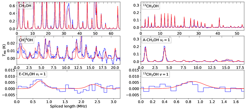
Figure 10: The blue lines are the spliced spectra of CH₃OH and its isotopologues as well as these species in vibrationally excited states. The spectrum between two neighbouring upper ticks are independent frequency segment. The red solid lines show the result of the model fitting of the corresponding species. The red dashed lines include the modeled emission of all species and RRLs. See Fig. 17 for other molecular species detected in the Ka-band survey.

The electron temperature ($T_{\rm e}$) can be estimated from the intensity ratios between RRLs and continuum (Gordon & Sorochenko, 2002), but can not be constrained by RRLs alone. Unfortunately, the continuum intensity was not well calibrated during our observations, and we have to assume a $T_{\rm e}$ to derive the emission measure. For RRLs from H II regions (neutral RRLs of H and He and ion RRLs), the $T_{\rm e}$ was fixed to be 8000 K (Wilson & Rood, 1994; Lerate et al., 2006). The $EM$ of H was then derived to be 1.5$\times$10⁶ cm^-6 pc, and the $EM$ of He is one tenth the value of H. The neutral RRLs of C mainly originate from the PDRs. Assuming a $T_{\rm e}$ of 300 K, the Ka-band spectra of the neutral RRLs of C can be reproduced by adopting an emission measure ($EM$) of 1.8$\times$10² cm^-2 pc (Figure 3). Table 2 of Liu et al. (2023) has already listed the fitted $EM$, velocity ($V_{\rm LSR}$), and line widths ($\Delta V$) of both neutral RRLs and ion RRLs basically based on this Ka-band survey of Orion KL, and thus will not be repeated in this work. In Liu et al. (2023), we briefly compared those parameters to justify the detection of ion RRLs of X⁺ with X referred to be C and/or O. Below, we will quote those parameters for more detailed analysis.

Figure 7 shows the intensity ratios between the observation and the model fitting ($T_{\rm obs}/T_{\rm model}$) for different transitions of H RRLs. For $\Delta n<10$, $T_{\rm obs}$ and $T_{\rm model}$ are consistent with each other within 50 percent, mainly contributed by the uncertainties of calibration and the different beam dilution at different frequencies. H96$\delta$ is an exception with a $T_{\rm obs}/T_{\rm model}$ of $\sim 1.6$. For $\Delta n>10$, the observed intensities tend to be lower than the model fitting. We do not know the specific reason for this discrepancy. One possibility is that the RRLs with large $\Delta n$ (and thus relatively large $n$ within a given frequency range) may deviate from LTE. Alternatively, RRLs with large $\Delta n$ tend to be weak, and the procedure of reducing spectral baseline through polynomial fitting may suppress broad and weak line features (Section 3.1). Further observations with higher S/Ns would help to explore this issue.

4.2 High-order neutral RRLs

Among the RRLs detected towards Orion KL in this survey, H148$\upsilon$ has the maximum $\Delta n$ of 20 (Figures 6 and 7). The line feature associated with H148$\upsilon$ has an intensity of larger than five sigma (Table 7), but it is slightly blended with two transitions of the vibrationally excited C₂H₅CN $\varv_{13}/\varv_{21}$ (Figure 6). Through modeling the emission of RRLs (Section 4.1) and C₂H₅CN $\varv_{13}/\varv_{21}$ (Section 5.2.2), we found that this line feature should be dominated by H148$\upsilon$ (Figure 6). For each $\Delta n<20$, there are one or more H RRLs that have been detected by this survey with intensities consistent with the model prediction (Figure 6). Thus, the detection of H148$\upsilon$ should be reliable. The maximum $\Delta n$ of this survey is the largest compared with previous blind line surveys at frequency bands (Ku, K, and Q) close to this survey (Table 3). Bell et al. (2011) reported the detection of a 2-$\sigma$ signal H RRLs with $\Delta n=25$ and a 3-$\sigma$ signal of H RRLs with $\Delta n=21$ (H274$\phi$) from a narrow-band (5.98–6.05 GHz) survey towards Orion KL using the NRAO 140-foot (43 m) telescope. RRLs tend to be weaker in the Ka band than in the C band. The broad bandwidth and much higher angular resolution of this survey enable us to detect spectrally resolved RRLs with a maximum $\Delta n$ close to that of Bell et al. (2011).

For He and C RRLs of this survey, the He147$o$ and C105$\epsilon$ reach the maximum $\Delta n$ of 15 and 5, respectively (Figure 6). Besides He147$o$, He114$\xi$ (with $\Delta n=14$ and $f_{\rm rest}=26866.5$ MHz) was also detected (Figure 3 and Table 7), and their intensities are consistent with those from LTE model. Thus, the line feature of He147$o$ is considered to be a firm detection under a 4$\sigma$ significance level (Table 7). The maximum $\Delta n$ of He and C RRLs of this survey are the largest compared with previous surveys towards Orion KL (Table 3).

4.3 High-order ion RRLs

Because of the blending with helium RRLs, the wide component ($\Delta V\sim 20$ km s^-1) of carbon RRLs originating from the ionized regions are difficult to be detected. The narrow component ($\Delta V\sim 5$ km s^-1; Table 2 of Liu et al. (2023)) of carbon RRLs can be spectrally resolved, but it traces the PDRs instead of the ionized regions. The PDRs traced by narrow C RRLs have a $V_{\rm LSR}$ of $\sim 8$ km s^-1, which is more than 10 km s^-1 redder than that of the ionized gas of M42 traced by H/He RRLs ($V_{\rm LSR}\sim-4$ km s^-1; Rizzo et al. 2017; Liu et al. 2023). The interaction between M42 and the molecular cloud may be responsible for the discrepancy of the $V_{\rm LSR}$ of PDRs located at the interface between them (Cuadrado et al., 2015; Rizzo et al., 2017). The ion RRLs provide us an opportunity to trace the doubly ionized element heavier than helium in the ionized regions. In Liu et al. (2023), only the $\alpha$ lines of RRLs of C⁺ and/or O⁺ were reported. There was no report of high-order ion RRLs (even for He⁺) with $\Delta n>1$ in the literature. The ionization energy of C II, 24.383 eV, is close to the value of He I, 24.587 eV, and thus the C III region should be comparable with the He II region in size. Thus, these $\alpha$ lines were assigned to C⁺ RRLs (Liu et al., 2023). However, the contribution of oxygen can not be excluded, because oxygen is as abundant as carbon, and the rest frequency shift between C⁺ and O⁺ RRLs is small ($\sim 3.5$ km s^-1). Interferometers may help to break the coupling between RRLs of C⁺ and O⁺ since they have different ionization energies (and therefore are presumably at different location), while single dish is difficult to distinguish them. Below, we tried to improve the S/Ns of ion RRLs through stacking, aiming to search for ion RRLs with $\Delta n>1$ from this Ka-band survey of the TMRT (Section 4.3.1) and to find signals of ion RRLs from independent telescopes beyond the TMRT (Section 4.3.2).

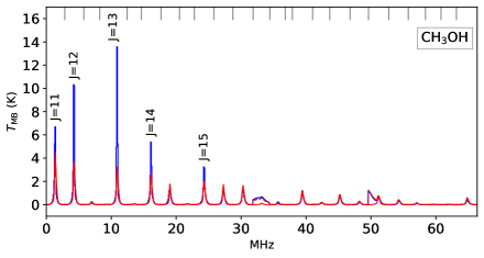
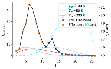
Figure 11: Left: The spliced spectrum of CH₃OH, same as the upper left panel of Figure 10, but with a different y-axis scale. The labeled transitions are $J_{K_{a},K_{c}}=J_{2,J-1}-J_{1,J-1}$. Right: The peak intensities ($I_{\rm peak}$) of CH₃OH $J_{2,J-1}-J_{1,J-1}$ detected in this survey (blue squares) and in the K-band survey of Gong et al. (2015) (orange squares). The red solid, gray dashed, and gray solid lines show the predicted peak intensity distribution along $J$ under LTE with a $T_{\rm ex}$ of 100 K, 200 K, and 50 K, respectively. The cyan line shows the rest frequency ($f_{0}$) of the transitions with different $J$.

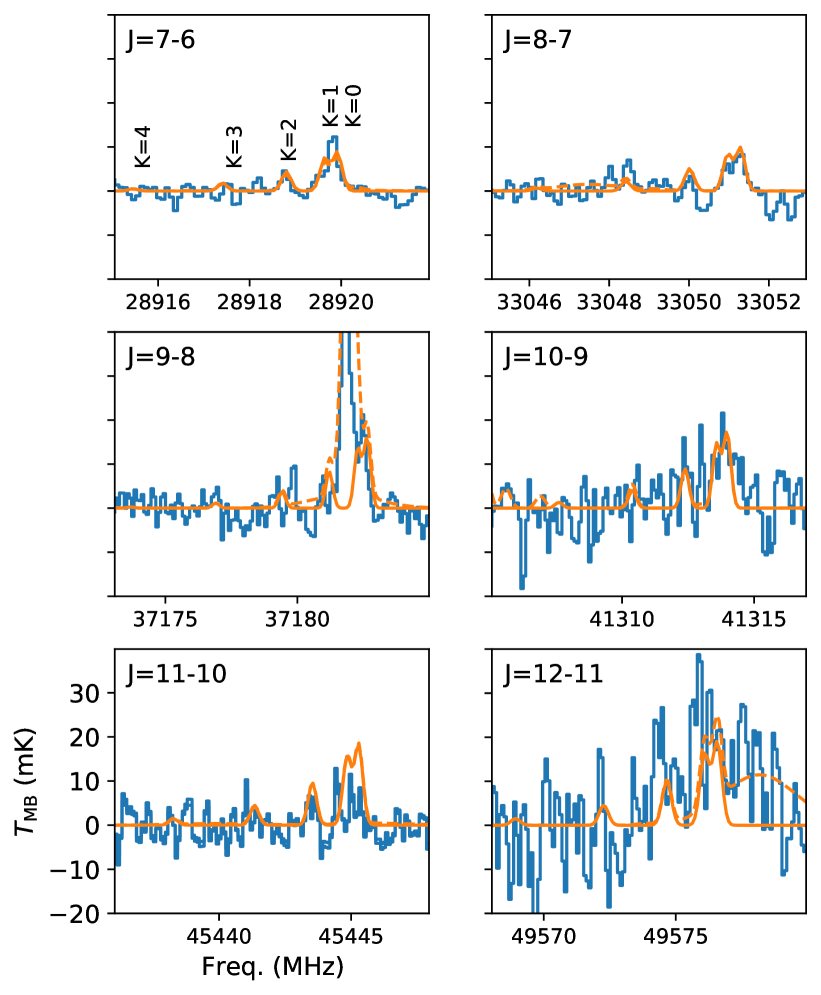
Figure 12: The spectra of CH₃C₃N (blue) in the Ka and Q bands. The y-axis in all panels have the same scale. Each rotational line is split into several transitions by the value of $K$, as marked in the upper-left panel. The orange solid lines are the model fitting of CH₃C₃N, and the orange dashed lines have taken all species into account. All transitions of CH₃C₃N expected to be stronger than 5 mK have been shown here.

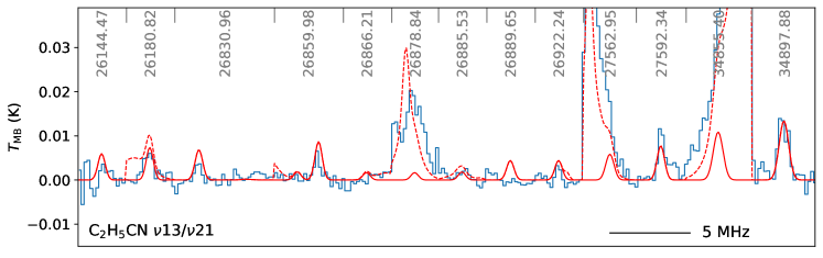
Figure 13: The spliced spectrum of C₂H₅CN $v_{13}/v_{21}$. The meaning of solid and dashed red lines are same as that of the upper left panel of Figure 10. The center frequencies of each segment are marked by the gray text labels.

4.3.1 Stacking of the Ka-band data of TMRT

For X⁺n$\beta$ with an even $n=2m$, Equation 1 leads to

$$\nu^{\rm RRL}_{\rm rest}(2m+2,2m) =\frac{m_{e}^{\prime}({\rm X})}{m_{e}}R_{\infty}c2^{2}\left(\frac{1}{(2m)^{2}}-\frac{1}{(2m+2)^{2}}\right)$$

$$\sim\frac{m_{e}^{\prime}({\rm He})}{m_{e}}R_{\infty}c\left(\frac{1}{(m)^{2}}-\frac{1}{(m+1)^{2}}\right),$$ (3)

and thus they should be blended with the $\alpha$ lines of neutral RRLs of helium (upper panel of Figure 8). For odd $n$, four $\beta$ lines of ion RRLs ($n=$ 125, 129, 117, and 115) show tentative line features. The 121$\beta$ and 123$\beta$ can not be recognized because of limited S/Ns, but do not contradict the model (Figure 8). Thus, it is very likely that we have detected the $\beta$ lines of ion RRLs.

To confirm the detection of $\beta$ lines and to search for higher-order ion RRLs, we stacked the spectra of different transitions to improve the S/N. We first check the Ka-band data, including both the observed and the modeled spectrum (Section 3.2), to select the spectral segments around the frequencies of ion RRLs (Equation 1) that are not blended by any other transitions within 20 km s^-1 (Figure 8). For a given $\Delta n$, we stacked all the corresponding unblended segments (with different $n$) aligned by velocity. The stacking was conducted with equal weights for different segments. The left panels of Figure 9 show the stacked Ka-band spectra of the $\alpha$, $\beta$ and $\gamma$ lines of ion RRLs.

It’s natural to see the high-S/N signal of the stacked $\alpha$ line since each unblended $\alpha$ line of ion RRLs can be clearly recognized (Liu et al., 2023). Besides the $\alpha$ lines, the stacked $\beta$ line shows clear detection (6$\sigma$; Figure 9), and the stacked $\gamma$ line shows very marginal signal. This is the first firm detection of ion RRLs with $\Delta n>1$ originated from the interstellar medium. We stacked the modeled data with the same procedure to obtain the stacked spectra (shown as the orange lines in Figure 9). In Liu et al. (2023), the fitting of ion RRLs was conducted based on $\alpha$ lines in three bands (Ku, Ka and Q). Here, we fitted them based on the Ka-band data only, but taking into account all the $\alpha$, $\beta$, and $\gamma$ lines. The fitted values of $EM$ (1.3$\times$10³ cm^-6 pc), the abundance of $X^{2+}$ (8.8$\times$10^-3) and the line width (17 km s^-1) are not altered compared with the values reported in Liu et al. (2023). The $V_{\rm LSR}$ fitted from the stacked spectra is -6.5 km s^-1 (with respect to the rest frequencies of C⁺ RRLs), slightly bluer than the value (-5.5 km s^-1) in Liu et al. (2023).

Comparing the relative intensities between the observation and model can provide an empirical test of the departures from LTE. The stacked $\gamma$ line seems to be slightly stronger than the modeled spectrum (bottom left panel of Figure 9), hinting at the deviation from LTE. However, the S/Ns of the stacked $\beta$ and $\gamma$ lines are not high enough to dig into this issue, and further observations with deeper sensitivities are needed to confirm it.

4.3.2 Comparison with the archived data of Effelsberg

We also checked the archive data of the K-band survey of Orion KL observed by Gong et al. (2015) using the Effelsberg 100 m telescope to search for the signals of ion RRLs. All $\alpha$ lines of ion RRLs in the K band can be recognized marginally or with moderate S/Ns, except for the blended X⁺109$\alpha$ and the X⁺102$\alpha$ which is located at the frequency gap of the K-band survey (see Appendix B and Figure 15). The intensities and velocities of the $\alpha$ lines of ion RRLs in the K band are consistent with the model prediction based on the Ka-band data. Using the same procedure in Section 4.3.1, we stacked the unblended ion RRLs in the K band. No clear signals of $\beta$ and $\gamma$ lines can be seen on the stacked spectra of the Effelsberg K-band survey because of the limited sensitivity. The signal of the $\alpha$ line can be clearly seen on the stacked spectrum (see the top right panel of Figure 9). This provides a very important cross check of ion RRLs from an independent facility.

5 Molecular lines

In total, 318 molecular lines were identified (Table 2), and they can be assigned to 37 species. Among them, 10 species (marked by ^(†) in Table 4) have no transitions being detected by the Q-band survey of the TMRT, because of the limited S/Ns or the lacking of transitions in the Q band. The vibrationally excited states ($v_{t}>0$) of nine species were detected, including the eight ones listed in Table 4 and C₂H₅CN $v_{13}/v_{21}$ (Section 5.2.2). For each detected transition, some transition parameters were quoted from the CDMS (Müller et al., 2001) and JPL (Pickett et al., 1998) through the Splatalogue . These parameters are the rest frequency ($f_{0}$), upper-level energy ($E_{\rm u}$), Einstein coefficients ($A_{ij}$), upper-level degeneracy ($g_{u}$), and partitial function ($Q$). The $f_{0}$ and $A_{ij}$ for transitions of C₂H₅CN $v13/v21$ were obtained from Endres et al. (2021). Through Equations 9, 10 and 11 of Liu et al. (2022), we modeled the emission of molecules. For most species, constraining $T_{\rm ex}$ is challenging due to the similar upper level energies of their different transitions. Therefore, $T_{\rm ex}$ is manually set to 50 K, 100 K, 150 K, 200 K, or, 300 K. We have also referred to the literature (Tercero et al., 2010; Gong et al., 2015; Rizzo et al., 2017; Liu et al., 2023) to choose proper $T_{\rm ex}$. To reproduce the emission of isotopologues or species with similar chemical characteristics, we tend to adopt the same fixed values of $T_{\rm ex}$, and use a similar initial guesses for their fitted parameters, including the column density ($N$), line width ($\Delta V$) and velocity ($V_{\rm LSR}$). We try to model the spectrum with as few velocity components as possible. The velocity resolution of the Ka-band survey is worse than that of the Q band, and species showing multiple velocity components may only show a single velocity component in the Ka band. For species detected in the Q band, if the modeled spectrum does not deviate much (less than 20 percent) from the observed spectrum in the Ka band, the number of the velocity components and the physical parameters fitted from the Q-band data will be directly used with no modification. The fitted parameters of molecular species are shown in Table 4.

5.1 Methanol emission

In total, 67 line features are assigned to methanol and its isotopologues, CH₃OH, ¹³CH₃OH, CH${}_{3}^{18}$OH, A-CH₃OH $v_{t}=1$, E-CH₃OH $v_{t}=1$, and ¹³CH₃OH $v_{t}=1$ (Figure 10). Among them, CH${}_{3}^{18}$OH and ¹³CH₃OH $v_{t}=1$ were not detected in the Q-band survey (Liu et al., 2022). Methanol contributes more about half the Ka-band molecular emission of Orion KL (Figure 5). Besides thermal components (Section 5.1.1), the maser emssion of methanol is also evident, as we discuss in Section 5.1.2.

Table 5: The species detected in the Ka-band survey

H${}^{+}{}^{(\dagger)}$	34SO	HCC13CN	CH3NH${}_{2}{}^{(*)}$	H${}_{2}^{13}$CO	CH3COCH3	CH${}_{3}^{18}$OH(‡)
He${}^{+}{}^{(\dagger)}$	SO2	HC3N $\varv_{6}=1$	CH3OH	H2CCO	NH3	HC7N(‡)
C${}^{+}{}^{(\dagger)}$	34SO2	HC3N $\varv_{7}=1$	13CH3OH	CH3CHO	NH2D	HDCO(‡)
X${}^{2+}{}^{(\dagger)}$	HCN $\varv_{2}=1$	HC3N $\varv_{7}=2$	A-CH3OH $\varv_{t}=1$	CH3OCHO	15NH${}_{3}{}^{(\ddagger)}$	18OCS(‡)
H2CS	HC3N	HC5N	E-CH3OH $\varv_{t}=1$	CH3OCHO $\varv_{t}=1$	13CH3OH $\varv=1{}^{(\ddagger)}$	33SO(‡)
CCS	H13CCCN	C2H3CN	C2H5OH	c-CH2OCH2	CH3C3N(‡)	c-C3H${}_{2}{}^{(\ddagger)}$
SO	HC13CCN	C2H5CN	H2CO	CH3OCH3	CH3CCH(‡)	C2H5CN $v_{13}/v_{21}$

Note: The species marked by ^(†) ions are traced by RRLs, e.g., X²⁺ was traced by X⁺ RRLs. The species marked by ^(‡) are detected in this Ka-band survey but not in the Q-band survey of TMRT. The species marked by ^(∗) are only tentatively detected.

5.1.1 Methanol thermal emission

We adopted three velocity components to fit the Ka-band spectra of CH₃OH under the assumption of LTE as in the Q band (Liu et al., 2022). The Ka-band emission of CH₃OH are dominated by strong lines ($T_{\rm peak}>1$ K), with sharp peaks that are not fully resolved under the current spectral resolution (the left panel of Figure 11). Thus, the emission of CH₃OH were reproduced with the narrow ($\Delta V=2$ km s^-1), moderate ($\Delta V=4$ km s^-1), and broad velocity components ($\Delta V=10$ km s^-1). Under the assumption of LTE, $T_{\rm ex}$ of the moderate component (150 K) is larger than that of the narrow component (100 K; Table 4). The column density ratio of CH₃OH/¹³CH₃OH and ¹³CH₃OH/CH${}_{3}^{18}$OH are 20 and 3.6, respectively. The CH₃OH/¹³CH₃OH is slightly larger than the values (5–15) of Rizzo et al. (2017), and smaller than the typical abundance ratio of Galactic ¹²C and ¹³C (several tens; Williams et al., 1994). This maser effects may influence this abundance ratio (Section 5.1.2). The ¹³CH₃OH/CH${}_{3}^{18}$OH is slightly lower than the abundance ratio of ¹³CO/C¹⁸O (X^13/18) in local ISM (Wilson, 1999; Shimajiri et al., 2014).

The spectral lines of CH₃OH $v_{t}=1$ (in both A and E asymmetry) have line widths of $\sim 4$ km s^-1. Adopting the excitation temperature ($T_{\rm ex}=$ 150 K) and the column density of the moderate component fitted from the emission of ¹³CH₃OH (Table 4), all line features of CH₃OH $v_{t}=1$ can be reproduced with a deviation no more than 10 percent (Figure 10). It implies that the vibrationally excited CH₃OH is mainly associated with the moderate component (instead of the narrow component). The narrow, moderate, and broad velocity components may originate from the compact ridge, hot core, and plateau, respectively (Rizzo et al., 2017).

5.1.2 Methanol masers

Several strong lines of CH₃OH ($T_{\rm peak}>3$ K) can not be successfully reproduced properly with any $T_{\rm ex}$ (Figure 11). Those lines belong to the same group of the transitions of E-type methanol (E-CH₃OH $J_{K_{a},K_{c}}=J_{2,J-1}-J_{1,J-1}$) with $11\leq J\leq 15$, and their rest frequencies are located within 26–29 GHz. It is consistent with the observations of Wilson et al. (1996), which detected narrow line components with $\Delta V\sim 0.8$ km s^-1 for $12\leq J\leq 17$ in the Ka band and assigned them to low gain maser regions. In Wilson et al. (1996), the peak intensity of the maser component is comparable with that of the thermal component. The observed intensity of the transition with $J=13$ by TMRT is four times stronger than the value of LTE prediction, showing the most significant deviation (Figure 11).

The transitions of E-CH₃OH in this group with $2\leq J\leq 9$ are well-known Class I maser transitions with rest frequencies located in the K band (Menten et al., 1986; Gong et al., 2015; Ladeyschikov et al., 2019). Combining the data of this work and Gong et al. (2015), we plotted the profile of the peak intensities ($I_{p}$) along $J$ with $2\leq J\leq 16$ in the right panel of Figure 11. Under the assumption of LTE, for compact source with an angular size smaller than the beam size, the profile of $I_{\rm peak}$ along $J$ can be calculated through

$$I_{p}\propto A_{ij}g_{u}\exp(-E_{u}/T_{\rm ex}).$$ (4)

Here, $E_{u}$ is in units of K. Three different values of $T_{\rm ex}$ (50, 100, and 200 K) were adopted, and all three profiles of $I_{p}$ can not fit all the Ka-band data points simultaneously (Figure 11). The data points with $J>15$ could be fitted adopting a $T_{\rm ex}$ of 100 K, and thus should be dominated by thermal emission. Note that the rest frequencies increase with $J$ for $J<20$, but decrease with $J$ for $J>20$ (see the cyan line in Figure 11). The rest frequency of the transition with a $J$ of 26 falls back to the K band, and its peak intensity is consistent with value extrapolated from the Ka-band data (Figure 11). Thus, the line of $J=26$ can be explained by the LTE fitting, consistent with the interpretation of Gong et al. (2015).

Previously, it is known that the maser effect would increase with $J$ from 2 to 6 and decrease with $J$ from 6 to 10 (Menten et al., 1986; Gong et al., 2015). The Ka-band data of this survey shows that the maser effect may increase with $J$ again from 11 to 13, and then decrease with $J$ from 13 to 15. These masers are likely class I methanol masers as well (Johnston et al., 1992; Wilson et al., 1996). The second peak can not simply be explained by the uncertainty of intensity calibration. The thermal lines of CH₃OH and other species in Ka band can all be well reproduced by the LTE model (Figures 3 and 10). Especially, the intensities of all the transitions of ¹³CH₃OH (upper right panel of Figure 10) are consistent with the LTE model within 20 percent (the calibration uncertainty; Section 2). To model the emission of ¹³CH₃OH, we adopted the same physical parameters as those for CH₃OH, except for the column densities, which have been scaled down (Table 4). The reason of the existence of two bumping peaks for E-CH₃OH $J_{K_{a},K_{c}}=J_{2,J-1}-J_{1,J-1}$, at $J\sim 6$ and $J\sim 13$, is still unknown. Interferometer observations are needed to confirm this issue through spatially resolving their different emission components.

5.2 N-bearing species

5.2.1 Methylcyanoacetylene (CH₃C₃N)

Methylcyanoacetylene (CH₃C₃N) was first detected in TMC-1 by Broten et al. (1984), with a column density of 4.5$\times$10¹¹ cm^-1 under a $T_{\rm ex}$ of 4 K (Lovas et al., 2006). It has also been detected in high-mass protostellar molecular clumps (Guzmán et al., 2018) and the Titan’s atmosphere (Thelen et al., 2020). However, CH₃C₃N has not been detected in Orion KL, even by the ALMA interferometer (Pagani et al., 2017).

In this Ka-band survey, we matched two groups of the emission lines of CH₃C₃N ($J=7-6$ and $J=8-7$; see Figure 17 and the upper two panels of Figure 12). The transitions of $K=0$ (blended with $K=1$) were detected for both groups. The transitions of K=2 ($E_{\rm u}\sim 35$ K) and K=3 ($E_{\rm u}\sim 75$ K) were tentatively detected. Thus, a $T_{\rm ex}$ of 50 K was adopted to fit the emission of CH₃C₃N, yielding a column density of 2$\times$10¹² cm^-2. Here, we assumed that the emission of CH₃C₃N is extended with a beam filling factor of unity. Further, we compared the modeled and observed spectra in the Q band, and found that they are also consistent with each other (Figure 12).

The fitted velocity ($V_{\rm LSR}$) is $9$ km s^-1, slightly redder than the systematic velocity (6 km s^-1) but consistent with that of CH₃CCH (Table 4), C RRLs (Section of 4.1), and the ambient gas of Orion KL (the extended ridge; Blake et al., 1986; Schilke et al., 1997). It implies that the CH₃C₃N emission of Orion KL may be associated with the PDRs or ambiment gas of Orion KL. This is reasonable since CH₃C₃N should be chemically young, given that it is an unsaturated species with its transitions mainly detected in chemically young environments, e.g., the starless core TMC-1 (Broten et al., 1984; Lovas et al., 2006).

5.2.2 Ethyl cyanide (C₂H₅CN)

Ethyl cyanide (C₂H₅CN) is a common tracer of hot molecular gas (e.g., Cazaux et al., 2003; Qin et al., 2022), and its vibrational satellites can be intense in sub-millimeter bands (Endres et al., 2021). In this survey, besides C₂H₅CN $v=0$, rotational transitions of C₂H₅CN $v_{13}/v_{21}$ (excited in bending or torsion modes; Daly et al., 2013) can also be detected (Figure 13). In total, four lines of C₂H₅CN $v_{13}/v_{21}$ were detected, less than the number of lines of C₂H₅CN $v_{13}/v_{21}$ detected in the Q band (Liu et al., 2022). Due to the higher spectral sensitivity of the Ka-band survey, the transition of C₂H₅CN $v_{13}/v_{21}$ at 34897.89 MHz, which was not detected in the Q band, can be clearly seen on the Ka-band spectrum (Figure 13). The other three transitions are located within 26–28 GHz. This marks the first detection of C₂H₅CN $v_{13}/v_{21}$ in the centimeter band.

To fit the emission of C₂H₅CN $v_{13}/v_{21}$, we adopted the transition parameters of C₂H₅CN $v_{13}/v_{21}$ from Endres et al. (2021) and assumed a $T_{\rm ex}$ of 50 K as in (Liu et al., 2022). Since we do not know the partition function, the column density can not be derived and the fitted parameters are thus not listed in Table 4. Here, we adopt the partition function of C₂H₅CN quoted from the CDMS. The velocity and line width are fitted to be 5 km s^-1 and 6 km s^-1, respectively, consistent with the result fitted from the Q-band data (Liu et al., 2022). The fitted column density of C₂H₅CN is 2$\times$10¹⁵ cm^-2. All transitions can be well fitted except for that in 26889 MHz. We not that this is not influenced by the $T_{\rm ex}$, because this transition and the strong line at 27592 MHz have similar $E_{u}$ ($\sim 300$ K).

5.2.3 Cyanopolyynes (HC_2n+1N)

Cyanopolyynes (HC_2n+1N) are abundant in kinds of environments, especially the cold cores (Herbst & Leung, 1989; Wu et al., 2019) and the envelopes of late-type carbon stars (Pardo et al., 2020), but not prominent in Orion KL. HC₇N was not detected by the Q-band (Liu et al., 2022) and K-band (Gong et al., 2015) line surveys of Orion KL. In this survey, spectral lines of HC₇N were detected with a peak intensity of $\sim$5 mK (Figure 17). The LTE fitting with a $T_{\rm ex}$ of 100 K yields a column density of 6$\times$10¹² cm^-2 and a $V_{\rm LSR}$ of 8.5 km s^-1. The $V_{\rm LSR}$ of HC_2n+1N is consistent with that of HC₅N (8.5 km s^-1), and the $V_{\rm LSR}$ of the reddest velocity component of HC₃N (9 km s^-1). The column density ratio of $N$(HC₃N)/$N$(HC₅N) is 35 (Table 4), close to the value derived by Gong et al. (2015), but much smaller than the column density ratio of $N$(HC₅N)/$N$(HC₇N), 6.6. However, if we only take the reddest velocity component of HC₃N into account, the abundance ratio of $N$(HC₃N)/$N$(HC₅N) would be 7.5, close to the value of $N$(HC₅N)/$N$(HC₇N). Thus, it is likely that the emission of HC₅N, HC₇N, and the reddest velocity component of HC₃N originates from the same region, probably the extended ridge of Orion KL.

5.2.4 Ammonia (NH₃ and NH₂D)

In total, 19 lines of ammonia were detected in this survey, including two lines of deuterated ammonia (NH₂D). Among them, NH₃ inversion line of $J_{K}=14_{13}$ (27772 MHz) has the highest $E_{\rm u}$ of 2090 K. The emission lines of NH₃ should be optically thick and we did not try to precisely fit them. To explain the high-$E_{\rm u}$ lines, a component with a $T_{\rm ex}$ of 300 K was adopted. Among the two lines of NH₂D, one is for the $para$-NH₂D (30979 MHz), and the other one for the $ortho$-NH₂D (29188 MHz). Under the equilibrium state, the abundance ratio of $ortho$-NH₂D/$para$-NH₂D ($o$/$p$) should be 3, the ratio of their statistical weights. When we fitted the NH₂D emission, the $T_{\rm ex}$ was fixed to be 300 K and the $o$/$p$ was fixed to be 3 since we did not distinguish the two types of NH₂D. Hence, the free parameters are only the column density ($N$), line width ($\Delta V$) and velocity ($V_{\rm LSR}$). The two lines can be fitted simultaneously (Figure 17), and thus the assumption of LTE should be acceptable. Only one line of ¹⁵NH₃ is detected, and the column density of ¹⁵NH₃ is calculated by adopting a $T_{\rm ex}$ of 300 K. The abundance ratio of NH₂D/¹⁵NH₃ is derived to be 4, but it highly depends on the $T_{\rm ex}$ and the assumption of LTE for ¹⁵NH₃.

5.3 Other species

For S-bearing species, ³³SO and ¹⁸OCS, which have not been detected in the Q-band survey of TMRT, were detected in the Ka band (Table 4). The abundance ratio of ³⁴SO/³³SO is derived to be 4.8, which does not deviate much from the value of Esplugues et al. (2013), $\sim$6.

All O-bearing complex organic molecules detected in this survey (Table 5), except for the isotopologues of CH₃OH (Section 5.1), have been detected by the Q-band survey of the TMRT (Liu et al., 2022). HDCO was not detected in the Q-band survey. For HDCO and H${}_{2}^{13}$CO, only one transition was detected for each in this survey. Adopting the same value of $T_{\rm ex}$ of 50 K, the abundance ratio of H${}_{2}^{13}$CO/HDCO is $\sim$1. Forty lines of CH₃OCH₃ were detected in this survey. In the Ka band, the total emission flux of CH₃OCH₃ is comparable with that of C₂H₅CN (Figure 5). In contrast, in the Q band, the total emission flux of CH₃OCH₃ is only 60 percent of that of C₂H₅CN. In the K band, only two lines of CH₃OCH₃ were detected by Gong et al. (2015). It implies that the Ka band has superiorities in detecting some species of complex organic molecules compared to the K and Q bands.

6 Summary

We have conducted a Ka-band line survey (26.1–35 GHz) towards Orion KL using the TMRT, following the Q-band survey with the same instrument (Liu et al., 2022). This survey achieved a line sensitivity of mK level (1–3 mK) at a spectral resolution of $\sim$1 km s^-1. This is the first blind line survey in the Ka band, and many transitions were detected for the first time. Further, we explore the Ka-band spectrum of Orion KL and present the overall preliminary results of the survey. The main results include:

• We have obtained and release the Ka-band spectrum of Orion KL by the TMRT. In the spectrum, 592 Gaussian features are detected in total, including 257 unblended RRLs and 318 unblended molecular lines. The maximum $\Delta n$ of RRLs of H, He, and C reach 20, 15, and 5, respectively. In total, 37 molecular species were detected, and the vibrationally excited states ($v_{t}>0$) of nine of these species were detected. Ten of these species have not been detected in the Q-band survey of TMRT, including CH₃C₃N which was not detected in Orion KL previsously even by ALMA. A catalog of these lines is presented.

• Through stacking, we have detected the $\beta$ lines of ion RRLs (RRLs of C⁺ and/or O⁺) for the first time, following our previous report of the $\alpha$ lines of ion RRLs. Tentative signal of the $\gamma$ lines of ion RRLs can be seen on the stacked spectrum. We also successfully matched the $\alpha$ lines of ion RRLs from the archive data of the K-band survey of Orion KL by the Effelsberg 100 m (Gong et al., 2015), providing a very important cross check of ion RRLs from an independent facility besides the TMRT.

• We modeled the spectral emission under the assumption of LTE. Parameters including the column densities ($N$) of molecular species and the emission measures ($EM$) of RRLs were derived. Adopting the precise values of the absorption oscillator strength of RRLs ($f_{n1,n2}$), the intensities of nearly all RRLs can be reproduced within a deviation of 50 percent. For $\Delta n>10$, the observed intensities tend to be slightly lower than model fitting.

• Most species can be well fitted under the assumption of LTE except for CH₃OH. The intensities of some transitions of E-CH₃OH $J_{2}-J_{1}$ can be at most four times the values of LTE prediction. The maser effect may explain this deviation (Wilson et al., 1996). Combining the data in Ka (this survey) and K band (Gong et al., 2015), we found that besides the bumping peak at $J\sim 6$, there is another one at $J\sim 13$.

Overall, this work emphasizes that the TMRT is able to conduct deep line surveys in the Ka band, and this band is very useful for surveying RRLs and molecular lines simultaneously.

Appendix A The absorption oscillator strength of RRLs

For hydrogenic RRL emitters, the absorption oscillator strength, $f_{n1,n2}$, is independent of $Z$ ignoring the effect of the slightly different reduced mass of electron (Kardashev, 1959; Goldwire & Goss, 1967). Menzel (1968) gave a useful approximation for the oscillator strength $f^{\star}_{n_{1},n_{2}}$ for RRLs:

$$f^{\star}_{n_{1},n_{2}}\sim n_{1}M_{\Delta n}\left(1+1.5\frac{\Delta n}{n_{1}}\right)$$ (A1)

In Liu et al. (2022), we empirically fitted the values of $M_{\Delta n}$ tabulated in Menzel (1968) as

$$M_{\Delta n}\sim 0.1905\left(1/\Delta n\right)^{2.887}$$ (A2)

Actually, the oscillator strength can be accurately calculated through the Gordon formula (Gordon, 1929). Following the Eqs. (3.1)–(3.7) of Brocklehurst (1971), we numerically tabulated the precise oscillator strength (denoted as $f^{{\dagger}}_{n1,n2}$) . The $\log_{10}(f^{{\dagger}}_{n_{1},n_{2}})$ and $f^{{\dagger}}_{n_{1},n_{2}}/f^{\star}_{n_{1},n_{2}}$ are shown in Figure 14. The $f^{\star}_{n_{1},n_{2}}$ deviates from $f^{{\dagger}}_{n_{1},n_{2}}$ by less than 20 percent when $\Delta n<5$.

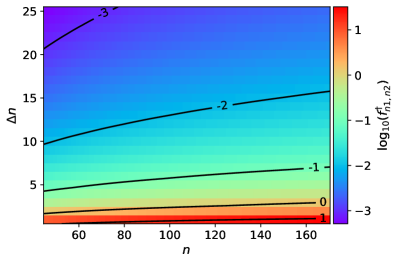
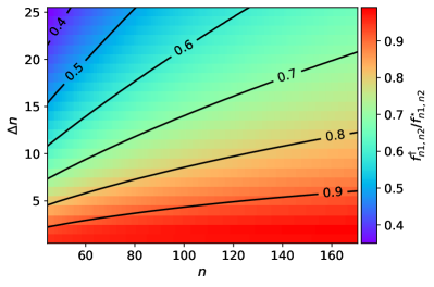
Figure 14: The $\log_{10}(f^{{\dagger}}_{n_{1},n_{2}})$ (left) and $f^{{\dagger}}_{n_{1},n_{2}}/f^{\star}_{n_{1},n_{2}}$ (right) for RRLs with different $n$ and $\Delta n$.

Appendix B The $\alpha$ lines of X⁺ RRLs in K band by Effelsberg

Figure 15 shows the $\alpha$ lines of ion RRLs from the archive data of the K-band survey of Orion KL by the Effelsberg 100 telescope (Gong et al., 2015). To exclude blending, we first modeled the K-band spectrum of Orion-KL. The RRLs are modeled using the parameters ($EM$, $\Delta V$, and $V_{\rm LSR}$) of this work. All molecular species detected in K band (Gong et al., 2015) can be detected in Q band (Liu et al., 2022) and Ka band (this work). Thus, to model the emission of molecular species, the parameters ($N$, $\Delta V$, $V_{\rm LSR}$ and $T_{\rm ex}$) obtained based on the Q-band and Ka-band data are used with no modification. Fortunately, most of the K-band $\alpha$ lines of ion RRLs are not blended (Figure 15).

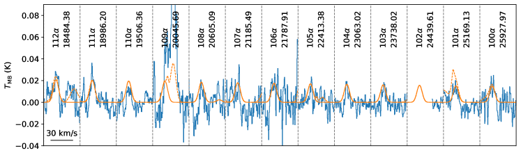
Figure 15: The K-band $\alpha$ lines of ion RRLs (blue) from the archive data of Effelsberg (Gong et al., 2015). The orange lines are the modeled spectrum. The orange dashed line takes all species into account, and the orange solid line only considers the ion RRLs.

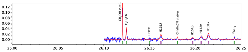
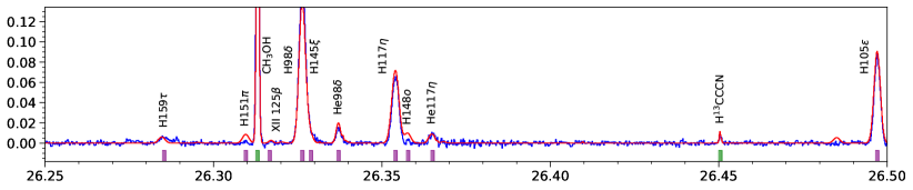
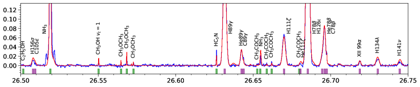
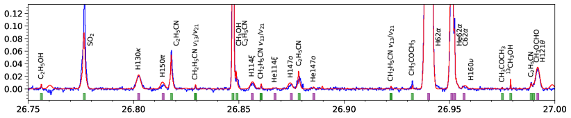
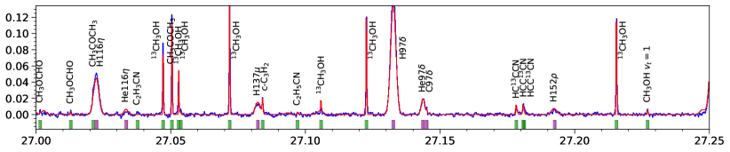
Figure 16: The Orion KL spectrum

Note: The blue line is the Orion KL spectrum observed by the TMRT 65 m, which has been smoothed to have a frequency resolution of 183 kHz ($\sim$1.8 km s^-1 at 30 GHz). The red line represents the modeling fitting. The purple strips denote the detected RRLs. The green strips denote the molecular lines. The gray strips mark the U lines.

Figure 16 (continued)

Note: The blue line is the Orion KL spectrum observed by the TMRT 65 m, which has been smoothed to have a frequency resolution of 183 kHz ($\sim$1.8 km s^-1 at 30 GHz). The red line represents the modeling fitting. The purple strips denote the detected RRLs. The green strips denote the molecular lines. The gray strips mark the U lines.

Figure 16 (continued)

Note: The blue line is the Orion KL spectrum observed by the TMRT 65 m, which has been smoothed to have a frequency resolution of 183 kHz ($\sim$1.8 km s^-1 at 30 GHz). The red line represents the modeling fitting. The purple strips denote the detected RRLs. The green strips denote the molecular lines. The gray strips mark the U lines.

Figure 16 (continued)

Note: The blue line is the Orion KL spectrum observed by the TMRT 65 m, which has been smoothed to have a frequency resolution of 183 kHz ($\sim$1.8 km s^-1 at 30 GHz). The red line represents the modeling fitting. The purple strips denote the detected RRLs. The green strips denote the molecular lines. The gray strips mark the U lines.

Figure 16 (continued)

Note: The blue line is the Orion KL spectrum observed by the TMRT 65 m, which has been smoothed to have a frequency resolution of 183 kHz ($\sim$1.8 km s^-1 at 30 GHz). The red line represents the modeling fitting. The purple strips denote the detected RRLs. The green strips denote the molecular lines. The gray strips mark the U lines.

Figure 16 (continued)

Note: The blue line is the Orion KL spectrum observed by the TMRT 65 m, which has been smoothed to have a frequency resolution of 183 kHz ($\sim$1.8 km s^-1 at 30 GHz). The red line represents the modeling fitting. The purple strips denote the detected RRLs. The green strips denote the molecular lines. The gray strips mark the U lines.

Figure 16 (continued)

Figure 16 continued

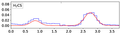
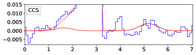
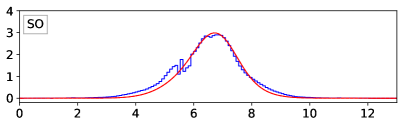
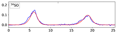
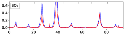
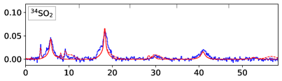
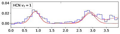
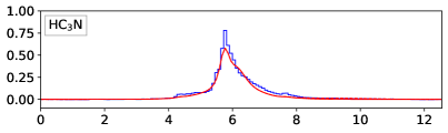
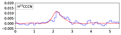
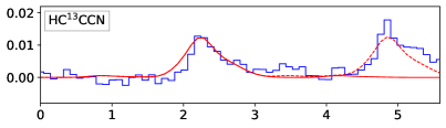
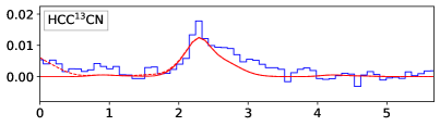
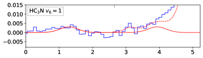
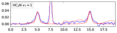
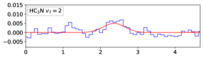
Figure 17: Model fitting for different species.

Note: In each panel, the spectra between two neighbouring upper ticks are independent frequency segments containing transitions of the corresponding species. The $x$ axis is in unit of MHz. The $y$ axis is $T_{\rm MB}$ in unit of K. See Figure 10 for the spliced spectra of methanol.

Figure 17 continued

Figure 17 (continued)

Figure 17 continued

Figure 17 (continued)

Figure 17 continued

Appendix C Line list of molecular lines

Table 6 shows the results of identification and Gaussian fitting of molecular lines, including RRLs which are blended with molecular lines. The unblended RRLs are listed in Table 7.
Table Notes:

• Doppler correction has been applied to $f_{\rm obs}$ assuming a source velocity of 6 km s^-1 in LSR (Sect. 3.1).
  Rows with empty $f_{\rm obs}$ correspond to blended lines.

• The emitter of ion RRL is denoted as X II, and the $f_{rest}$ is adopted as the rest frequency of the corresponding C II RRL.
  The unidentified species is denoted as U.

• Rows with a same species name and transition label correspond to different emission components of a same transition.
  The transition labels for HCN $\varv_{t}=1$ are $J^{p}$ with $p$ the parity.
  The transition labels for CH₃OCH₃ are $J_{K}^{s}$ with $s$ the symmetry substate.
  The transition labels are $(J,K)$ for NH₃ convention lines.

• The numbers in brackets in the 7th and 8th columns represent the uncertainties of the last digital of corresponding parameters.
  

Table 6: Linelist

$f_{\rm obs}$	Species	$f_{\rm rest}$	Transition	$E_{u}$	$A_{ij}$	$\int{T_{\rm MB}}{\rm d}V$	$\Delta$V	$T_{\rm MB}^{\rm peak}$	$V_{\rm LSR}$
(MHz)		(MHz)	$J_{K_{a},K_{c}}$	(K)	(10-6 s-1)	(K km s-1)	(km s-1)	K	km s-1
26120.55	CH3OH $\varv_{t}=1$	26120.584	$10_{1,9}-11_{2,9}$	452.7	0.06	0.879(9)	4(1)	1.93E$-$01	6.4(1)
26124.84	C2H5CN	26124.592	$3_{1,3}-2_{1,2}$	3.6	1.17	0.507(9)	13(1)	3.72E$-$02	3(1)
26149.88	HDCO	26150.160	$8_{2,6}-8_{2,7}$	144.3	0.06	0.021(2)	2(1)	8.16E$-$03	9(1)
26180.75	C2H5CN $\varv 13$/$\varv 21$	26180.635		299.8	0.06	0.049(9)	8(1)	5.95E$-$03	5(1)
26242.78	15NH3	26242.760	$J_{K}=9_{9}-9_{9}$	852.5	0.4	0.078(9)	6(1)	1.18E$-$02	6(1)
26289.13	U					0.050(2)	8(1)	5.60E$-$03
26313.06	E-CH3OH	26313.192	$11_{2,10}-11_{1,10}$	175.5	0.1	9.09(2)	6.4(1)	1.33E$+$00	7.5(1)
26450.51	H13CCCN	26450.596	$J=3-2$	2.5	1.28	0.088(7)	8.8(9)	9.47E$-$03	7.0(3)
26501.59	C2H5OH	26501.778	$4_{1,3}-4_{2,3}$	71.3	0.06	0.009(2)	1.3(6)	7.07E$-$03	8.1(1)
26516.55	NH3	26518.981	($8_{8}$,$8_{8}$)	686.8	0.4	0.291(6)	10.5(2)	2.59E$-$02	33.5(2)
26519.11	NH3	26518.981	($8_{8}$,$8_{8}$)	686.8	0.4	8.05(1)	9.1(1)	8.33E$-$01	4.5(1)
26521.59	NH3	26518.981	($8_{8}$,$8_{8}$)	686.8	0.4	0.40(1)	12.1(3)	3.13E$-$02	-23.5(1)
26550.22	CH3OH $\varv_{t}=1$	26550.263	$10_{9,2}-10_{8,2}$	811.0	0.03	0.051(5)	3.1(3)	1.56E$-$02	6.5(1)
26564.72	CH3OCH3	26564.800	$12_{3,9}^{\rm 0}-11_{4,8}^{\rm 0}$	83.9	0.02	0.024(4)	2.2(4)	1.03E$-$02	6.9(1)
26568.43	CH3OCH3	26568.544	$12_{3,9}^{\rm 1}-11_{4,8}^{\rm 1}$	83.9	0.02	0.103(5)	3.1(2)	3.14E$-$02	7.3(1)
26572.76	CH3OCH3	26572.820	$12_{3,9}^{\rm 12}-11_{4,8}^{\rm 12}$	83.9	0.02	0.035(5)	3.5(6)	9.48E$-$03	6.6(1)
26626.35	HC5N	26626.463	$J=10-9$	7.0	1.96	0.124(5)	3.7(2)	3.15E$-$02	7.2(1)
26652.59	AE-CH3COCH3	26652.524	$11_{7,4}-11_{6,5}$	54.3	0.7	0.009(2)	4(2)	2.35E$-$03	5(1)
26654.18	NH3	26654.847	($13_{12}$,$13_{12}$)	1826.0	0.4	0.237(6)	31(1)	7.12E$-$03	14(1)
26654.93	NH3	26654.847	($13_{12}$,$13_{12}$)	1826.0	0.4	0.094(6)	4(1)	2.01E$-$02	5(1)
26658.75	AA-CH3COCH3	26658.734	$11_{7,4}-11_{6,5}$	54.1	0.7	0.023(6)	3(1)	6.28E$-$03	6(1)
26661.94	EE-CH3COCH3	26661.943	$11_{7,4}-11_{6,5}$	54.2	0.7	0.056(5)	5.0(5)	1.06E$-$02	6.1(2)
26679.70	EA-CH3COCH3	26679.716	$11_{7,4}-11_{6,5}$	54.3	0.7	0.021(6)	4(2)	4.81E$-$03	6.2(8)
26756.26	C2H5OH	26756.342	$1_{1,0}-1_{0,1}$	2.1	0.2	0.048(2)	4(1)	1.07E$-$02	7(1)
26776.61	SO2	26776.574	$25_{4,22}-24_{5,19}$	339.0	0.04	2.25(1)	16.3(1)	1.30E$-$01	5.6(1)
26818.02	C2H5CN	26817.814	$3_{0,3}-2_{0,2}$	2.6	1.43	0.68(1)	11(1)	5.57E$-$02	4(1)
26829.40	C2H5CN $\varv 13$/$\varv 21$	26829.333		307.8	1.43	0.037(8)	6(2)	5.37E$-$03	5.3(5)
26847.20	E-CH3OH	26847.237	$12_{2,11}-12_{1,11}$	203.4	0.1	26.6(1)	2.0(1)	1.24E$+$01	6.4(1)
26849.09	C2H5CN	26848.630	$3_{2,2}-2_{2,1}$	7.0	0.8	0.37(2)	19(1)	1.84E$-$02	0.8(5)
26860.54	C2H5CN $\varv 13$/$\varv 21$	26860.453		298.9	0.8	0.023(4)	2.6(5)	8.53E$-$03	5.0(2)
26878.65	C2H5CN	26878.303	$3_{2,1}-2_{2,0}$	7.0	0.8	0.42(1)	23.4(9)	1.71E$-$02	2.2(4)
26880.43	U					0.036(7)	3.6(7)	9.41E$-$03
26922.22	C2H5CN $\varv 13$/$\varv 21$	26922.076		302.9	0.8	0.014(3)	2.5(7)	5.17E$-$03	4.4(3)
26932.38	EE-CH3COCH3	26932.441	$12_{8,4}-12_{7,5}$	64.5	0.8	0.094(4)	6.2(4)	1.43E$-$02	6.7(2)
26975.10	AA-CH3COCH3	26974.959	$12_{8,4}-12_{7,5}$	64.4	0.8	0.024(6)	6(3)	3.76E$-$03	4(2)
26979.06	13CH3OH	26979.070	$12_{4,9}-13_{3,10}$	257.4	0.03	0.019(5)	3(1)	6.29E$-$03	6(1)
26988.82	C2H5CN	26988.679	$5_{1,4}-5_{0,5}$	7.7	0.2	0.11(3)	9(4)	1.16E$-$02	4(3)
26989.98	A-CH3OCHO	26989.976	$7_{2,5}-6_{3,4}$	19.7	0.006	0.033(9)	5(1)	6.25E$-$03	6(1)
27001.51	A-CH3OCHO	27001.548	$18_{10,9}-19_{9,10}$	167.3	0.004	0.033(9)	4(1)	8.04E$-$03	6(1)
27012.87	E-CH3OCHO	27012.953	$7_{2,5}-6_{3,4}$	19.7	0.005	0.016(4)	3(1)	5.10E$-$03	7(1)
27021.22	AA-CH3COCH3	27021.085	$9_{7,2}-9_{6,3}$	38.5	0.6	0.1633(2)	11.0(6)	1.40E$-$02	4.5(1)
27037.69	C2H3CN	27037.600	$21_{2,19}-21_{2,20}$	114.9	0.03	0.04(1)	10(4)	4.20E$-$03	5(2)
27047.17	13CH3OH	27047.280	$3_{2,1}-3_{1,2}$	35.9	0.09	0.37(1)	3(1)	1.04E$-$01	7(1)
27050.43	13CH3OH	27050.540	$4_{2,2}-4_{1,3}$	45.0	0.1	0.47(1)	3(1)	1.40E$-$01	7(1)
27052.89	13CH3OH	27053.030	$2_{2,0}-2_{1,1}$	29.2	0.07	0.18(1)	3(1)	5.37E$-$02	8(1)
27053.76	EE-CH3COCH3	27053.621	$9_{7,2}-9_{6,3}$	38.6	0.5	0.029(8)	5(1)	4.98E$-$03	4(1)
27071.87	13CH3OH	27071.930	$5_{2,3}-5_{1,4}$	56.3	0.1	0.582(5)	3.4(1)	1.60E$-$01	6.6(1)
27084.14	c-C3H2	27084.352	$3_{3,0}-3_{2,1}$	19.5	1.0	0.077(8)	4.0(4)	1.82E$-$02	8.3(1)
27097.05	C2H5CN	27097.100	$26_{4,23}-25_{5,20}$	169.0	0.03	0.015(4)	4(2)	3.44E$-$03	6.5(8)
27105.83	13CH3OH	27105.870	$12_{4,8}-13_{3,11}$	257.4	0.03	0.042(7)	5(1)	7.32E$-$03	6.4(1)
27122.67	13CH3OH	27122.720	$6_{2,4}-6_{1,5}$	69.9	0.1	0.554(5)	3.3(1)	1.60E$-$01	6.6(1)
27178.34	HC13CCN	27178.505	$J=3-2$	2.6	1.39	0.056(5)	4.2(5)	1.23E$-$02	7.9(1)
27180.87	HCC13CN	27180.885	$J=3-2$	2.6	1.17	0.031(7)	2.5(4)	1.17E$-$02	6.1(1)
27181.27	HCC13CN	27181.151	$J=3-2$	2.6	1.23	0.11(1)	11(1)	8.92E$-$03	4.7(6)
27215.52	13CH3OH	27215.570	$7_{2,5}-7_{1,6}$	85.8	0.1	0.537(4)	3.5(1)	1.44E$-$01	6.6(1)
27227.06	CH3OH $\varv_{t}=1$	27227.113	$6_{3,3}-7_{2,5}$	466.0	0.004	0.032(5)	4.2(8)	7.15E$-$03	6.6(3)
27283.11	E-CH3OH	27283.140	$14_{5,10}-15_{4,12}$	367.6	0.03	0.83(4)	4.5(3)	1.73E$-$01	6.3(1)
27292.95	HC3N	27294.289	$J=3-2$	2.6	1.41	0.68(2)	11(1)	5.88E$-$02	21(1)
27294.20	HC3N	27294.289	$J=3-2$	2.6	1.41	6.08(7)	11.0(2)	5.20E$-$01	7.0(1)
27295.12	HC3N	27294.289	$J=3-2$	2.6	1.41	1.33(2)	13(1)	9.60E$-$02	-3(1)
27296.05	HC3N	27294.289	$J=3-2$	2.6	1.41	0.20(2)	6(1)	3.05E$-$02	-13(1)
27296.90	H140$\nu$	27296.730				0.30(2)	18(1)	1.59E$-$02	4(1)
	HC3N	27296.233	$J=3-2$	2.6	0.07				-1(1)
27339.00	HC3N $\varv_{6}=1$	27339.150	$J=3-2$	720.3	1.26	0.028(5)	9(1)	3.07E$-$03	8(1)
27349.42	EA-CH3COCH3	27349.349	$9_{7,2}-9_{6,3}$	38.7	0.5	0.014(3)	3(1)	4.09E$-$03	5(1)
27359.68	C2H5OH	27359.801	$6_{3,4}-6_{2,4}$	85.3	0.06	0.009(2)	1.7(6)	4.66E$-$03	7.3(3)
27361.45	HC3N $\varv_{7}=1$	27361.410	$J=3-2$	323.5	1.26	0.30(2)	21(2)	1.33E$-$02	5.6(5)
27361.59	HC3N $\varv_{7}=1$	27361.410	$J=3-2$	323.5	1.26	0.16(2)	7.6(6)	1.97E$-$02	4.0(2)
27364.01	C2H5CN	27363.777	$9_{3,6}-10_{2,9}$	29.4	0.03	0.541(4)	3.5(1)	1.45E$-$01	3.4(1)
27390.72	U					0.025(6)	6(2)	3.75E$-$03
27400.78	HC3N $\varv_{7}=1$	27400.630	$J=3-2$	323.5	1.26	0.45(1)	12(1)	3.37E$-$02	4(1)
27467.79	HC3N $\varv_{7}=2$	27467.677	$J=3-2$	644.3	1.43	0.035(5)	5.5(9)	5.96E$-$03	4.7(5)
27470.95	E-CH3OH	27470.972	$25_{2,24}-25_{1,24}$	776.2	0.05	0.155(4)	3.8(1)	3.84E$-$02	6.2(1)
27472.50	E-CH3OH	27472.534	$13_{2,12}-13_{1,12}$	233.6	0.1	25.5(1)	1.7(1)	1.41E$+$01	6.4(1)
27475.58	NH3	27477.943	($9_{9}$,$9_{9}$)	852.8	0.5	0.34(1)	13.0(7)	2.46E$-$02	31.7(2)
27478.06	NH3	27477.943	($9_{9}$,$9_{9}$)	852.8	0.5	7.55(3)	9.1(1)	7.81E$-$01	4.7(1)
27480.65	NH3	27477.943	($9_{9}$,$9_{9}$)	852.8	0.5	0.159(8)	9.9(6)	1.51E$-$02	-23.6(2)
27549.13	EA-CH3COCH3	27549.108	$6_{5,2}-6_{4,3}$	18.3	0.4	0.013(3)	10(7)	1.25E$-$03	6(4)
27555.56	H${}_{2}^{13}$CO	27555.673	$3_{1,2}-3_{1,3}$	32.9	0.1	0.26(1)	4(1)	5.65E$-$02	7(1)
27561.85	C2H5CN	27561.680	$3_{1,2}-2_{1,1}$	3.8	1.38	0.58(1)	11(1)	5.08E$-$02	4(1)
27562.79	C2H5CN	27561.680	$3_{1,2}-2_{1,1}$	3.8	1.38	0.20(1)	14(1)	1.30E$-$02	-6(1)
27581.55	13CH3OH	27581.630	$9_{2,7}-9_{1,8}$	124.3	0.1	0.53(1)	3(1)	1.52E$-$01	6.8(1)
27592.40	C2H5CN $\varv 13$/$\varv 21$	27592.228		300.0	0.1	0.06(1)	4.8(9)	1.23E$-$02	4.1(9)
27593.23	U					0.05(1)	8.1(9)	5.40E$-$03
27625.55	CH3OCH3	27625.739	$2_{2,1}^{\rm 12}-3_{1,2}^{\rm 12}$	8.4	0.01	0.010(2)	1.8(8)	5.28E$-$03	8.0(4)
27627.54	CH3OCH3	27627.573	$2_{2,1}^{\rm 11}-3_{1,2}^{\rm 11}$	8.4	0.02	0.031(6)	5(2)	5.51E$-$03	6.4(6)
27629.39	CH3OCH3	27629.487	$2_{2,1}^{\rm 1}-3_{1,2}^{\rm 1}$	8.4	0.01	0.036(4)	2.7(4)	1.26E$-$02	7.0(2)
27632.31	CH3OCH3	27632.353	$2_{2,1}^{\rm 0}-3_{1,2}^{\rm 0}$	8.4	0.01	0.023(3)	1.0(9)	2.14E$-$02	6.5(2)
27700.15	CH3OH $\varv_{t}=1$	27700.180	$12_{2,11}-11_{1,11}$	479.2	0.07	0.9393(4)	4.4(1)	1.99E$-$01	6.3(1)
27767.58	C2H3CN	27767.351	$3_{1,3}-2_{1,2}$	4.8	1.38	0.142(9)	9.9(7)	1.35E$-$02	3.5(2)
	H167$\omega$	27767.269							2.7(2)
27772.30	NH3	27772.294	($14_{13}$,$14_{13}$)	2090.5	0.4	0.040(6)	7(1)	5.18E$-$03	5.9(4)
27817.42	CH3OH $\varv_{t}=1$	27817.439	$11_{9,3}-11_{8,3}$	836.5	0.04	0.066(8)	4.2(9)	1.48E$-$02	6.2(9)
27820.81	E-CH3OH	27820.841	$19_{5,14}-18_{6,13}$	576.7	0.03	0.335(8)	4.4(9)	7.09E$-$02	6.3(9)
27879.98	13CH3OH	27880.030	$10_{2,8}-10_{1,9}$	147.0	0.1	0.462(8)	3.4(9)	1.29E$-$01	6.6(9)
27919.48	C2H5OH	27919.726	$3_{0,3}-2_{1,2}$	5.0	0.09	0.026(7)	10(3)	2.48E$-$03	9(2)
27932.26	SO2	27932.411	$25_{2,24}-24_{3,21}$	303.7	0.02	1.02(1)	24.4(4)	3.92E$-$02	7.6(2)
27932.56	SO2	27932.411	$25_{2,24}-24_{3,21}$	303.7	0.02	0.31(1)	6.6(2)	4.41E$-$02	4.4(1)
27992.91	13CH3OH	27992.990	$6_{2,5}-5_{3,2}$	85.4	0.02	0.033(4)	2.3(3)	1.32E$-$02	6.9(1)
28014.07	C2H5OH	28014.169	$2_{1,1}-2_{0,2}$	3.9	0.3	0.046(6)	4.0(7)	1.09E$-$02	7.0(2)
28050.20	EE-CH3COCH3	28050.283	$6_{5,2}-6_{4,3}$	18.2	0.5	0.021(4)	3.1(6)	6.49E$-$03	6.9(3)
28069.16	E-CH3OH	28069.208	$16_{0,16}-15_{3,13}$	327.6	0.0006	0.041(3)	2.7(2)	1.43E$-$02	6(1)
28120.03	C2H5OH	28120.258	$5_{3,3}-5_{2,3}$	80.3	0.06	0.012(3)	2.8(9)	4.06E$-$03	8.4(4)
28122.17	C2H5CN	28122.144	$19_{5,14}-20_{4,17}$	109.5	0.03	0.019(4)	2.1(5)	8.31E$-$03	5.7(1)
28137.17	13CH3OH	28137.250	$6_{2,4}-5_{3,3}$	85.4	0.02	0.13(1)	6.8(9)	1.80E$-$02	6.8(2)
28138.20	C109$\zeta$	28138.816				0.11(1)	12(2)	8.46E$-$03	12.6(9)
	SO2 $v_{2}=1$	28138.394	$4_{0,4}-3_{1,3}$	754.2	0.1				8.1(9)
28143.03	CH3NH2	28142.850	$J_{K}=18_{1}-18_{0}$	363.8	0.3	0.012(3)	3(1)	3.75E$-$03	4.1(5)
28169.43	E-CH3OH	28169.470	$14_{2,13}-14_{1,13}$	266.1	0.1	13.06(3)	2.2(1)	5.66E$+$00	6.4(1)
28173.64	C2H5CN	28173.414	$18_{2,16}-18_{2,17}$	79.0	0.04	0.042(8)	7(2)	5.35E$-$03	3.6(7)
	SO2 $v_{2}=1$	28173.485	$8_{2,6}-9_{1,9}$	788.5	0.04				4.4(7)
28199.57	HC7N	28199.798	$J=25-24$	17.6	2.97	0.019(4)	3.4(7)	5.28E$-$03	8.4(4)
28239.53	A-CH3OCHO	28239.630	$9_{2,8}-8_{3,5}$	28.8	0.005	0.023(6)	2.5(8)	8.44E$-$03	7.1(3)
28261.46	E-CH3OCHO	28261.511	$9_{2,8}-8_{3,5}$	28.8	0.005	0.020(5)	3(1)	6.56E$-$03	6.6(3)
28267.70	13CH3OH	28267.770	$11_{2,9}-11_{1,10}$	171.9	0.1	0.449(5)	3.5(1)	1.20E$-$01	6.7(1)
28315.98	E-CH3OH	28316.067	$4_{0,4}-3_{1,2}$	36.3	0.04	5.96(1)	4.4(1)	1.28E$+$00	6.9(1)
28329.43	AA-CH3COCH3	28329.300	$6_{5,2}-6_{4,3}$	18.2	0.5	0.025(6)	7(2)	3.55E$-$03	4.7(9)
28338.41	EE-CH3COCH3	28338.466	$11_{8,3}-11_{7,4}$	55.5	0.8	0.062(6)	5.1(6)	1.15E$-$02	6.6(2)
28344.05	U					0.018(5)	3(1)	5.58E$-$03
28407.67	AA-CH3COCH3	28407.350	$11_{8,3}-11_{7,4}$	55.5	0.8	0.047(7)	3.8(6)	1.16E$-$02	2.7(2)
28406.53	A-CH3OCHO	28406.628	$21_{8,14}-20_{9,11}$	179.2	0.005	0.008(2)	1.7(6)	4.36E$-$03	7.0(3)
28441.12	C2H3CN	28441.026	$3_{0,3}-2_{0,2}$	2.7	1.67	0.163(8)	10.5(7)	1.45E$-$02	5.1(1)
28456.12	C2H3CN	28455.983	$3_{2,2}-2_{2,1}$	11.4	0.8	0.028(7)	8(2)	3.15E$-$03	5(1)
28457.31	C2H3CN	28457.201	$3_{2,2}-2_{2,1}$	11.4	0.9	0.046(6)	5.4(9)	8.11E$-$03	4.9(3)
28543.11	H152$\sigma$	28541.838				0.041(7)	9(2)	4.36E$-$03	-7.4(8)
	C2H5OH	28543.098	$4_{3,2}-4_{2,2}$	76.2	0.06				5.9(8)
28596.85	AA-CH3COCH3	28596.855	$10_{6,4}-10_{5,5}$	44.7	0.8	0.023(5)	4(1)	4.99E$-$03	6.1(5)
28602.30	NH3	28604.737	($10_{10}$,$10_{10}$)	1036.4	0.5	0.070(7)	8(1)	8.36E$-$03	31.5(4)
28604.85	NH3	28604.737	($10_{10}$,$10_{10}$)	1036.4	0.5	3.04(2)	7.2(1)	3.99E$-$01	4.9(1)
28607.45	NH3	28604.737	($10_{10}$,$10_{10}$)	1036.4	0.5	0.093(7)	13(1)	6.92E$-$03	-22.4(5)
28616.08	A-CH3OCHO $\varv_{t}=1$	28616.175	$5_{1,4}-5_{0,5}$	197.8	0.04	0.037(8)	6.2(9)	5.67E$-$03	7.0(9)
28620.92	EE-CH3COCH3	28620.971	$10_{6,4}-10_{5,5}$	44.8	0.8	0.060(8)	5.1(9)	1.10E$-$02	6.5(9)
28622.50	C2H5CN	28622.275	$6_{1,5}-6_{0,6}$	10.4	0.2	0.114(8)	8.7(9)	1.23E$-$02	3.6(9)
28629.96	AE-CH3COCH3	28629.885	$5_{2,3}-5_{1,4}$	11.6	0.5	0.014(3)	3.8(9)	3.43E$-$03	5.2(9)
28636.53	A-CH3OCHO $\varv_{t}=1$	28636.634	$9_{2,7}-9_{2,8}$	217.8	0.03	0.009(2)	5(3)	1.78E$-$03	7(1)
28660.21	EA-CH3COCH3	28660.137	$10_{6,4}-10_{5,5}$	44.9	0.8	0.010(2)	1.8(7)	4.90E$-$03	5.3(3)
28671.15	EE-CH3COCH3	28671.065	$5_{2,3}-5_{1,4}$	11.5	0.5	0.018(5)	5(2)	3.49E$-$03	5.1(9)
28692.57	A-CH3OCHO $\varv_{t}=1$	28692.722	$25_{6,19}-25_{6,20}$	405.0	0.03	0.007(2)	1.7(6)	4.16E$-$03	7.6(4)
28705.65	AA-CH3COCH3	28705.700	$5_{2,3}-5_{1,4}$	11.4	0.5	0.022(5)	3.7(9)	5.57E$-$03	6.5(9)
28747.66	13CH3OH	28747.750	$12_{2,10}-12_{1,11}$	199.1	0.1	0.366(5)	3.4(9)	1.00E$-$01	7.0(9)
28857.98	SO2	28858.037	$17_{2,16}-16_{3,13}$	149.2	0.04	12.64(2)	21.6(1)	5.50E$-$01	6.6(1)
28874.37	E-CH3OH	28874.394	$24_{2,23}-24_{1,23}$	718.4	0.07	0.33(1)	4.0(9)	7.78E$-$02	6.2(9)
28905.76	E-CH3OH	28905.812	$15_{2,14}-15_{1,14}$	301.0	0.1	10.23(2)	2.9(1)	3.31E$+$00	6.6(1)
28919.86	CH3C3N	28919.927	$J_{K}=7_{1}-6_{1}$	13.0	2.90	0.037(5)	2.9(6)	1.18E$-$02	6.7(2)
28969.90	A-CH3OH	28969.959	$8_{2,7}-9_{1,8}$	121.3	0.05	6.13(7)	5.0(1)	1.16E$+$00	6.6(1)
28974.67	H2CO	28974.805	$3_{1,2}-3_{1,3}$	33.4	0.1	13.08(7)	4.4(1)	2.82E$+$00	7.4(1)
29091.20	CH3OCH3	29091.288	$3_{0,3}^{\rm 0}-2_{1,2}^{\rm 0}$	5.4	0.08	0.170(7)	2.9(9)	5.59E$-$02	6.9(9)
29092.01	CH3OCH3	29092.090	$3_{0,3}^{\rm 1}-2_{1,2}^{\rm 1}$	5.4	0.08	0.270(7)	3.0(9)	8.34E$-$02	6.9(9)
29092.81	CH3OCH3	29092.895	$3_{0,3}^{\rm 12}-2_{1,2}^{\rm 12}$	5.4	0.08	0.180(7)	3.3(9)	5.06E$-$02	6.9(9)
29113.83	CH3OH $\varv_{t}=1$	29113.793	$12_{9,4}-12_{8,4}$	864.3	0.05	0.083(8)	4.5(9)	1.72E$-$02	5.7(9)
29139.34	C2H3CN	29139.199	$3_{1,2}-2_{1,1}$	5.0	1.34	0.084(8)	5.8(9)	1.35E$-$02	4.6(9)
29187.74	NH2D	29187.763	$7_{2,6}-7_{1,6}$	460.5	0.3	0.186(8)	5.4(9)	3.21E$-$02	6.2(9)
29255.89	C2H5OH	29255.814	$5_{1,4}-5_{2,4}$	75.6	0.08	0.032(9)	6(3)	5.29E$-$03	5.2(7)
29266.84	C2H5OH	29266.907	$5_{1,4}-6_{0,6}$	75.6	0.06	0.015(4)	4(1)	3.79E$-$03	6.7(6)
29288.97	HC5N	29289.152	$J=11-10$	8.4	2.62	0.29(1)	6.2(3)	4.50E$-$02	7.9(1)
	X II96$\alpha$	29287.782							-6.1(1)
29293.01	H2CS	29293.210	$7_{1,6}-7_{1,7}$	60.0	0.01	0.088(7)	3.8(3)	2.14E$-$02	8.0(1)
29315.14	13CH3OH	29315.200	$13_{2,11}-13_{1,12}$	228.6	0.2	0.335(9)	3.5(1)	8.99E$-$02	6.6(1)
29321.20	SO2	29321.330	$4_{0,4}-3_{1,3}$	9.2	0.1	27.25(2)	22.7(1)	1.13E$+$00	7.3(1)
29327.71	HC7N	29327.768	$J=26-25$	19.0	3.35	0.031(7)	5(1)	6.19E$-$03	6.6(6)
29401.45	E-CH3OCHO	29401.796	$5_{1,4}-5_{0,5}$	10.0	0.04	0.082(6)	2.9(3)	2.69E$-$02	9.5(1)
29417.40	A-CH3OCHO	29417.462	$5_{1,4}-5_{0,5}$	10.0	0.04	0.089(5)	2.7(2)	3.07E$-$02	6.7(1)
29429.90	H2CCO	29430.020	$12_{1,11}-12_{1,12}$	89.4	0.004	0.014(4)	2.9(8)	4.65E$-$03	7.2(4)
29460.48	C2H5CN	29460.274	$15_{2,13}-14_{3,12}$	56.6	0.04	0.032(6)	6(1)	5.43E$-$03	3.9(6)
29584.77	HCN $\varv_{2}=1$	29584.660	$11^{+}-11^{-}$	1306.4	0.02	0.137(6)	5.5(3)	2.33E$-$02	4.9(1)
29625.17	A-CH3OCHO	29625.340	$12_{4,8}-11_{5,7}$	57.0	0.007	0.024(4)	4.5(8)	4.93E$-$03	7.7(4)
29636.89	E-CH3OH	29636.942	$16_{2,15}-16_{1,15}$	338.1	0.2	5.99(1)	4.4(1)	1.29E$+$00	6.5(1)
29678.73	34SO	29678.980	$N_{J}=0_{1}-1_{0}$	1.4	0.2	3.34(1)	23.5(1)	1.33E$-$01	8.5(1)
29686.97	c-CH2OCH2	29687.030	$5_{4,1}-5_{3,2}$	33.0	0.4	0.047(4)	2.4(2)	1.83E$-$02	6.6(1)
29741.51	E-CH3OCHO	29741.570	$12_{4,8}-11_{5,7}$	57.0	0.004	0.010(2)	1.9(8)	4.73E$-$03	6.6(4)
29819.85	33SO	29819.833	$N_{J}=0_{1}-1_{0}$	1.4	0.2	0.20(1)	19(2)	9.97E$-$03	5.8(8)
29857.34	33SO	29857.602	$N_{J}=0_{1}-1_{0}$	1.4	0.2	0.44(2)	25(2)	1.62E$-$02	8.6(6)
29900.40	CH3OCH3	29900.479	$1_{1,0}^{\rm 11}-1_{0,1}^{\rm 11}$	2.3	0.3	0.24(1)	3.3(9)	6.80E$-$02	6.8(9)
29901.30	CH3OCH3	29901.394	$1_{1,0}^{\rm 1}-1_{0,1}^{\rm 1}$	2.3	0.3	0.35(1)	2.8(9)	1.19E$-$01	6.9(9)
29902.20	CH3OCH3	29902.300	$1_{1,0}^{\rm 0}-1_{0,1}^{\rm 0}$	2.3	0.3	0.21(1)	2.8(9)	7.19E$-$02	7.0(9)
29914.02	NH3	29914.486	($11_{11}$,$11_{11}$)	1237.6	0.6	0.99(2)	34(1)	2.70E$-$02	10.6(6)
29914.57	NH3	29914.486	($11_{11}$,$11_{11}$)	1237.6	0.6	1.37(1)	5.8(1)	2.22E$-$01	5.1(1)
29955.64	13CH3OH	29955.700	$14_{2,12}-14_{1,13}$	260.3	0.2	0.275(8)	3.7(1)	6.91E$-$02	6.6(1)
29979.28	C2H5OH	29979.381	$3_{1,2}-3_{0,3}$	6.5	0.3	0.057(7)	4.0(5)	1.34E$-$02	7.0(1)
30001.38	SO	30001.580	$N_{J}=0_{1}-1_{0}$	1.4	0.2	69.67(5)	24.0(1)	2.73E$+$00	8.0(1)
30005.99	EE-CH3COCH3	30006.173	$13_{9,4}-13_{8,5}$	75.8	1.0	0.14(1)	8.6(9)	1.57E$-$02	7.8(3)
30010.43	A-CH3OH	30010.511	$8_{1,7}-8_{1,8}$	98.8	0.003	0.854(8)	3.7(1)	2.14E$-$01	6.8(1)
30205.52	SO2	30205.549	$16_{2,14}-17_{1,17}$	137.5	0.01	2.11(1)	19.2(2)	1.04E$-$01	6.2(1)
30218.76	X II95$\alpha$	30217.519				0.18(1)	15(2)	1.14E$-$02	-6.3(6)
	SO2	30218.740	$56_{10,46}-55_{11,45}$	1714.7	0.07				5.8(6)
30307.99	E-CH3OH	30308.033	$17_{2,16}-17_{1,16}$	377.6	0.2	4.423(4)	4.2(1)	9.89E$-$01	6.5(1)
30429.89	CH3OH $\varv_{t}=1$	30429.883	$13_{9,5}-13_{8,5}$	894.4	0.06	0.056(7)	4.1(6)	1.28E$-$02	6.0(3)
30521.34	C2H5OH	30521.578	$7_{3,4}-7_{2,6}$	91.1	0.08	0.012(3)	3(2)	3.58E$-$03	8.3(9)
30559.66	A-CH3OCHO	30559.815	$5_{1,4}-4_{2,3}$	10.0	0.01	0.013(3)	1.2(9)	1.02E$-$02	7.5(9)
30564.01	E-CH3OCHO	30564.097	$5_{1,4}-4_{2,3}$	10.0	0.01	0.019(5)	2.4(9)	7.65E$-$03	6.9(9)
30606.89	C2H5CN	30606.460	$7_{1,6}-7_{0,7}$	13.4	0.2	0.37(1)	18(1)	1.92E$-$02	1.8(4)
30643.66	13CH3OH	30643.720	$15_{2,13}-15_{1,14}$	294.3	0.2	0.251(8)	4.4(2)	5.42E$-$02	6.6(1)
30670.51	E-CH3OCHO	30670.582	$9_{2,7}-9_{2,8}$	30.2	0.03	0.087(7)	2.7(3)	3.04E$-$02	6.7(1)
30695.08	A-CH3OCHO	30695.155	$9_{2,7}-9_{2,8}$	30.2	0.03	0.071(6)	2.9(3)	2.27E$-$02	6.7(1)
30752.19	E-CH3OH	30752.222	$22_{2,21}-22_{1,21}$	609.6	0.1	0.80(2)	4.3(8)	1.74E$-$01	6.3(8)
30858.25	E-CH3OH	30858.301	$18_{2,17}-18_{1,17}$	419.4	0.2	3.419(8)	4.6(1)	6.96E$-$01	6.5(1)
30966.48	CH3OCH3	30966.551	$5_{3,3}^{\rm 12}-6_{2,4}^{\rm 12}$	26.3	0.02	0.027(7)	5(2)	4.94E$-$03	6.7(8)
30973.04	CH3OCH3	30973.137	$5_{3,3}^{\rm 1}-6_{2,4}^{\rm 1}$	26.3	0.03	0.084(6)	2.7(2)	2.89E$-$02	6.9(1)
30975.31	34SO2	30975.450	$8_{1,7}-7_{2,6}$	36.6	0.09	0.60(1)	15.7(5)	3.60E$-$02	7.4(2)
30977.00	34SO2	30975.450	$8_{1,7}-7_{2,6}$	36.6	0.09	0.244(7)	76(8)	3.03E$-$03	-9(6)
30978.77	NH2D	30978.726	$6_{2,5}-6_{1,5}$	353.4	0.4	0.072(7)	3.7(4)	1.80E$-$02	5.6(2)
31011.01	34SO2	31011.180	$4_{0,4}-3_{1,3}$	9.1	0.2	0.93(2)	24.8(7)	3.51E$-$02	7.6(3)
31011.23	34SO2	31011.180	$4_{0,4}-3_{1,3}$	9.1	0.2	0.18(2)	6.8(5)	2.44E$-$02	5.5(2)
31090.06	SO2	31089.928	$28_{3,25}-29_{2,28}$	403.0	0.01	0.16(1)	9.4(7)	1.60E$-$02	4.7(3)
31105.14	CH3OCH3	31105.220	$2_{1,1}^{\rm 11}-2_{0,2}^{\rm 11}$	4.2	0.3	0.171(6)	2.4(1)	6.61E$-$02	6.8(1)
31106.05	CH3OCH3	31106.150	$2_{1,1}^{\rm 1}-2_{0,2}^{\rm 1}$	4.2	0.3	0.442(7)	2.5(1)	1.63E$-$01	6.9(1)
31106.98	CH3OCH3	31107.077	$2_{1,1}^{\rm 0}-2_{0,2}^{\rm 0}$	4.2	0.3	0.168(6)	2.4(1)	6.50E$-$02	7.0(1)
31209.74	E-CH3OH	31209.778	$21_{2,20}-21_{1,20}$	558.6	0.1	1.107(9)	4.2(1)	2.48E$-$01	6.3(1)
31226.70	E-CH3OH	31226.750	$19_{2,18}-19_{1,18}$	463.5	0.2	2.51(1)	4.5(1)	5.22E$-$01	6.5(1)
31306.58	AA-CH3COCH3	31306.546	$14_{9,5}-14_{8,6}$	86.2	1.19	0.06(1)	8(2)	7.61E$-$03	5.7(8)
31342.24	13CH3OH	31342.280	$16_{2,14}-16_{1,15}$	330.6	0.2	0.141(8)	3.7(3)	3.61E$-$02	6.4(1)
31358.37	E-CH3OH	31358.415	$20_{2,19}-20_{1,19}$	509.9	0.1	1.729(9)	4.5(1)	3.61E$-$01	6.4(1)
31365.36	U					0.054(9)	7(1)	7.13E$-$03
31425.02	NH3	31424.943	($12_{12}$,$12_{12}$)	1456.4	0.7	1.42(1)	8.0(1)	1.68E$-$01	5.3(1)
31573.34	C2H5CN	31573.070	$34_{8,26}-35_{7,29}$	327.0	0.04	0.021(5)	6(2)	3.39E$-$03	3(1)
31723.66	AA-CH3COCH3	31723.622	$9_{5,4}-9_{4,5}$	36.1	0.9	0.019(2)	4.3(8)	4.29E$-$03	5.6(8)
31739.47	EE-CH3COCH3	31739.498	$9_{5,4}-9_{4,5}$	36.2	0.9	0.021(2)	2.7(8)	7.48E$-$03	6.3(8)
31740.92	AE-CH3COCH3	31740.723	$9_{5,4}-9_{4,5}$	36.3	0.9	0.011(2)	2.4(8)	4.35E$-$03	4.1(8)
31757.35	CH3OH $\varv_{t}=1$	31757.390	$14_{9,5}-14_{8,7}$	926.8	0.07	0.049(2)	4.6(8)	9.89E$-$03	6.4(8)
31816.99	13CH3OH $\varv_{t}=1$	31817.070	$10_{1,10}-11_{2,9}$	449.5	0.1	0.013(3)	2.0(5)	5.83E$-$03	6.8(3)
31898.49	C2H5CN	31898.305	$1_{1,1}-0_{0,0}$	1.5	0.2	0.035(7)	9(2)	3.69E$-$03	4(1)
31918.00	C2H5OH	31917.978	$11_{1,10}-10_{2,8}$	114.2	0.06	0.021(4)	4.6(9)	4.23E$-$03	5.8(5)
31922.19	SO2	31922.210	$16_{4,12}-17_{3,15}$	164.5	0.08	6.25(2)	25.6(1)	2.29E$-$01	6.1(1)
31922.25	SO2	31922.210	$16_{4,12}-17_{3,15}$	164.5	0.08	1.47(2)	8.1(1)	1.69E$-$01	5.6(1)
31951.59	HC5N	31951.772	$J=12-11$	10.0	3.42	0.139(4)	3.7(1)	3.55E$-$02	7.7(1)
31977.74	E-CH3OH	31977.791	$19_{4,15}-20_{3,18}$	536.7	0.06	0.593(5)	4.1(1)	1.36E$-$01	6.5(1)
31996.01	CH3OCH3	31996.105	$9_{2,7}^{\rm 0}-8_{3,6}^{\rm 0}$	47.0	0.04	0.099(5)	2.6(2)	3.55E$-$02	6.8(1)
31999.27	CH3OCH3	31999.357	$9_{2,7}^{\rm 1}-8_{3,6}^{\rm 1}$	47.0	0.04	0.151(5)	2.5(1)	5.75E$-$02	6.8(1)
32002.48	CH3OCH3	32002.458	$9_{2,7}^{\rm 11}-8_{3,6}^{\rm 11}$	47.0	0.04	0.117(7)	5.0(3)	2.19E$-$02	5.8(1)
32004.29	13CH3OH	32004.340	$17_{2,15}-17_{1,16}$	369.1	0.2	0.131(6)	3.9(2)	3.15E$-$02	6.4(1)
32071.92	HDCO	32072.200	$3_{1,2}-3_{1,3}$	27.3	0.2	0.136(4)	3.5(1)	3.61E$-$02	8.6(1)
32190.88	EE-CH3COCH3	32190.958	$7_{5,3}-7_{4,4}$	23.1	0.8	0.044(8)	7(2)	5.88E$-$03	6.7(6)
32206.02	E-CH3OCHO	32206.029	$29_{7,22}-29_{7,23}$	293.6	0.04	0.060(3)	10.3(8)	5.51E$-$03	6.1(8)
32253.38	A-CH3OCHO	32253.467	$29_{7,22}-29_{7,23}$	293.6	0.04	0.016(3)	1.8(4)	8.26E$-$03	6.8(2)
32272.86	He104$\zeta$	32272.195				0.12(1)	17(2)	6.45E$-$03	-0.2(8)
	34SO2	32272.340	$25_{6,20}-26_{5,21}$	383.8	0.08				1.2(8)
32355.87	U					0.028(5)	3.0(5)	8.65E$-$03
32379.35	CH3OH $\varv_{t}=1$	32379.386	$21_{5,17}-20_{6,15}$	954.7	0.09	0.068(4)	3.0(2)	2.10E$-$02	6.3(1)
32398.40	13CH3OH	32398.480	$4_{1,4}-3_{0,3}$	28.3	0.1	0.410(4)	3.1(1)	1.22E$-$01	6.7(1)
32454.46	U					0.015(3)	2.1(6)	6.71E$-$03
32485.99	E-CH3CHO	32486.053	$8_{1,7}-7_{2,6}$	36.5	0.03	0.008(2)	1.4(7)	5.70E$-$03	6.6(2)
32539.19	AA-CH3COCH3	32538.241	$15_{10,5}-15_{9,6}$	99.1	1.34	0.027(4)	2.9(5)	8.81E$-$03	-2.8(2)
32570.78	C2H5OH	32570.883	$6_{1,5}-6_{2,5}$	80.7	0.1	0.015(4)	4(1)	3.44E$-$03	7.0(6)
32575.47	13CH3OH	32575.520	$18_{2,16}-18_{1,17}$	409.9	0.2	0.074(3)	3.1(2)	2.27E$-$02	6.5(1)
32612.83	E-CH3OCHO	32613.143	$42_{10,32}-42_{10,33}$	607.1	0.04	0.010(2)	3.7(8)	2.57E$-$03	8.9(8)
32708.79	A-CH3CHO	32709.214	$4_{0,4}-3_{1,3}$	9.2	0.08	0.018(5)	5(2)	3.33E$-$03	9.9(8)
32742.71	C2H5OH	32742.830	$4_{1,3}-4_{0,4}$	9.9	0.4	0.077(5)	4.4(4)	1.67E$-$02	7.1(1)
32837.25	AA-CH3COCH3	32837.510	$13_{8,5}-13_{7,6}$	74.2	1.26	0.047(7)	5(1)	8.50E$-$03	8.4(4)
32873.07	EE-CH3COCH3	32873.058	$13_{8,5}-13_{7,6}$	74.3	1.26	0.053(8)	6(1)	7.81E$-$03	5.9(5)
32973.45	C2H5CN	32973.250	$8_{1,7}-8_{0,8}$	17.0	0.3	0.22(1)	9.9(5)	2.12E$-$02	4.2(2)
32977.18	CH3OCH3	32977.277	$3_{1,2}^{\rm 12}-3_{0,3}^{\rm 12}$	7.0	0.3	0.348(6)	2.4(1)	1.35E$-$01	6.9(1)
32978.13	CH3OCH3	32978.232	$3_{1,2}^{\rm 1}-3_{0,3}^{\rm 1}$	7.0	0.3	0.523(6)	2.5(1)	2.00E$-$01	7.0(1)
32979.08	CH3OCH3	32979.187	$3_{1,2}^{\rm 0}-3_{0,3}^{\rm 0}$	7.0	0.3	0.330(6)	2.4(1)	1.29E$-$01	7.0(1)
32998.89	13CH3OH	32998.850	$19_{2,17}-19_{1,18}$	452.9	0.2	0.074(5)	3.9(3)	1.77E$-$02	5.7(1)
33044.38	EE-CH3COCH3	33044.425	$8_{7,1}-8_{6,2}$	32.1	0.5	0.008(2)	1.6(8)	5.00E$-$03	6.4(8)
33051.23	CH3C3N	33051.619	$J_{K}=8_{0}-7_{0}$	7.1	4.46	0.039(6)	4.8(7)	7.72E$-$03	9.5(4)
33156.63	NH3	33156.849	($13_{13}$,$13_{13}$)	1692.7	0.8	0.37(1)	24(1)	1.47E$-$02	8.0(5)
33156.94	NH3	33156.849	($13_{13}$,$13_{13}$)	1692.7	0.8	0.17(1)	4.4(2)	3.56E$-$02	5.2(1)
33164.19	E-CH3OCHO	33164.204	$6_{1,5}-6_{1,6}$	13.7	0.03	0.057(5)	2.9(3)	1.88E$-$02	6.1(1)
33186.11	A-CH3OCHO	33186.266	$6_{1,5}-6_{1,6}$	13.7	0.03	0.046(5)	2.8(3)	1.54E$-$02	7.4(1)
33212.83	34SO2	33212.810	$17_{2,16}-16_{3,13}$	148.5	0.06	0.394(4)	21.2(8)	1.75E$-$02	5.8(8)
33219.98	13CH3OH	33220.080	$20_{2,18}-20_{1,19}$	498.2	0.2	0.036(4)	4.3(8)	7.83E$-$03	6.9(8)
33329.26	CH3OCH3	33329.338	$8_{4,5}^{\rm 12}-9_{3,6}^{\rm 12}$	55.3	0.02	0.013(3)	1.7(8)	6.85E$-$03	6.7(8)
33336.63	CH3OCH3	33336.805	$8_{4,5}^{\rm 11}-9_{3,6}^{\rm 11}$	55.3	0.04	0.071(3)	7.5(8)	8.84E$-$03	7.6(8)
33337.53	CH3OCH3	33337.611	$8_{4,5}^{\rm 1}-9_{3,6}^{\rm 1}$	55.3	0.03	0.070(3)	2.6(8)	2.50E$-$02	6.7(8)
33344.13	CH3OCH3	33344.224	$8_{4,5}^{\rm 0}-9_{3,6}^{\rm 0}$	55.3	0.04	0.050(3)	2.6(8)	1.79E$-$02	6.9(8)
33348.25	CH3OCH3	33348.357	$8_{4,4}^{\rm 1}-9_{3,6}^{\rm 1}$	55.3	0.010	0.027(3)	3.1(8)	8.28E$-$03	6.9(8)
33366.26	E-CH3OCHO	33366.394	$10_{2,9}-9_{3,6}$	34.5	0.007	0.034(3)	5.8(8)	5.48E$-$03	7.2(8)
33376.37	CH3OCH3	33376.636	$5_{3,3}^{\rm 1}-6_{2,5}^{\rm 1}$	26.3	0.002	0.053(3)	7.4(8)	6.68E$-$03	8.4(8)
33386.70	U					0.018(4)	2.1(5)	7.80E$-$03
33392.62	CH3OCH3	33392.739	$5_{3,2}^{\rm 11}-6_{2,5}^{\rm 11}$	26.3	0.03	0.028(2)	2.3(8)	1.13E$-$02	7.0(8)
33397.33	CH3OCH3	33397.481	$5_{3,2}^{\rm 1}-6_{2,5}^{\rm 1}$	26.3	0.03	0.098(2)	3.7(8)	2.47E$-$02	7.3(8)
33399.54	CH3OCH3	33399.668	$5_{3,2}^{\rm 0}-6_{2,5}^{\rm 0}$	26.3	0.03	0.051(2)	2.8(8)	1.70E$-$02	7.2(8)
33446.89	C2H5CN	33446.898	$19_{2,17}-19_{2,18}$	87.3	0.06	0.068(8)	12.6(8)	5.06E$-$03	6.1(8)
33508.38	C2H5OH	33508.434	$2_{1,2}-1_{1,1}$	65.2	0.2	0.007(2)	0.9(4)	7.20E$-$03	6.5(2)
33555.64	AE-CH3COCH3	33555.523	$3_{0,3}-2_{1,2}$	3.7	1.26	0.015(4)	2.1(7)	6.72E$-$03	5.0(3)
33566.38	AA-CH3COCH3	33566.289	$3_{0,3}-2_{1,2}$	3.5	1.26	0.031(8)	5(1)	6.29E$-$03	5.2(1)
33630.14	C2H5CN	33629.960	$6_{0,6}-5_{1,5}$	9.0	0.1	0.102(2)	11.9(8)	8.04E$-$03	4.4(8)
33691.60	A-CH3OH	33691.663	$23_{5,19}-24_{4,20}$	777.9	0.07	0.079(2)	3.0(8)	2.47E$-$02	6.6(8)
33751.28	CCS	33751.370	$N_{J}=2_{3}-1_{2}$	3.2	1.58	0.027(4)	4.8(8)	5.27E$-$03	6.8(8)
33904.06	A-CH3OCHO $\varv_{t}=1$	33904.211	$3_{1,3}-2_{1,2}$	191.8	0.5	0.054(6)	2.7(8)	1.85E$-$02	7.4(8)
33918.87	CH${}_{3}^{18}$OH	33919.030	$2_{2,0}-2_{1,1}$	29.1	0.04	0.031(6)	4(1)	6.80E$-$03	7.4(3)
33925.37	CH${}_{3}^{18}$OH	33925.510	$3_{2,1}-3_{1,2}$	35.7	0.04	0.083(6)	4.2(8)	1.88E$-$02	7.2(8)
33932.24	CH3OCH3	33932.378	$8_{4,5}^{\rm 1}-9_{3,7}^{\rm 1}$	55.3	0.01	0.022(6)	2.7(8)	7.62E$-$03	7.3(8)
33936.41	CH3OCH3	33936.516	$8_{4,4}^{\rm 11}-9_{3,7}^{\rm 11}$	55.3	0.04	0.032(6)	3.0(8)	1.02E$-$02	6.9(8)
33943.00	CH3OCH3	33943.123	$8_{4,4}^{\rm 1}-9_{3,7}^{\rm 1}$	55.3	0.03	0.080(6)	3.6(8)	2.10E$-$02	7.1(8)
33943.74	CH3OCH3	33943.924	$8_{4,4}^{\rm 0}-9_{3,7}^{\rm 0}$	55.3	0.04	0.125(6)	5.6(8)	2.08E$-$02	7.6(8)
33981.26	CH${}_{3}^{18}$OH	33981.400	$5_{2,3}-5_{1,4}$	55.8	0.05	0.054(5)	3.5(5)	1.45E$-$02	7.2(1)
34003.42	A-CH3OH	34003.457	$23_{5,18}-24_{4,21}$	777.9	0.07	0.123(7)	4.5(3)	2.57E$-$02	6.3(1)
34048.26	CH${}_{3}^{18}$OH	34048.422	$6_{2,4}-6_{1,5}$	69.1	0.05	0.048(5)	2.7(3)	1.67E$-$02	7.4(1)
34092.91	EE-CH3COCH3	34092.973	$3_{1,3}-2_{0,2}$	3.6	1.35	0.025(5)	3.2(6)	7.40E$-$03	6.6(3)
34097.71	SO2	34097.720	$26_{6,20}-27_{5,23}$	411.4	0.09	0.656(7)	21.2(8)	2.90E$-$02	6.1(8)
34097.87	SO2	34097.720	$26_{6,20}-27_{5,23}$	411.4	0.09	0.360(7)	5.6(8)	6.00E$-$02	4.7(8)
34100.07	H2CO	34100.050	$10_{2,8}-10_{2,9}$	240.7	0.09	0.349(7)	7.3(8)	4.51E$-$02	5.8(8)
34147.62	c-CH2OCH2	34147.720	$4_{4,0}-4_{3,1}$	23.3	0.4	0.028(7)	1.6(8)	1.60E$-$02	6.8(8)
34155.55	CH${}_{3}^{18}$OH	34155.634	$7_{2,5}-7_{1,6}$	84.7	0.05	0.026(4)	1.9(4)	1.29E$-$02	6.8(1)
34156.78	E-CH3OCHO	34156.884	$3_{1,3}-2_{1,2}$	4.0	0.5	0.27(2)	2.6(3)	9.66E$-$02	6.9(1)
34157.96	A-CH3OCHO	34158.119	$3_{1,3}-2_{1,2}$	3.9	0.5	0.28(3)	2.8(3)	9.33E$-$02	7.4(1)
34160.53	E-CH3OCHO $\varv_{t}=1$	34160.654	$3_{1,3}-2_{1,2}$	191.0	0.5	0.05(1)	3(2)	1.48E$-$02	7.1(9)
34182.43	CH3CCH	34182.760	$J_{K}=2_{1}-1_{1}$	9.7	0.09	0.156(4)	2.6(1)	5.67E$-$02	8.9(1)
34183.11	CH3CCH	34183.414	$J_{K}=2_{0}-1_{0}$	2.5	0.1	0.332(7)	4.0(1)	7.75E$-$02	8.7(1)
34212.56	EE-CH3COCH3	34212.823	$8_{6,3}-8_{5,4}$	30.3	1.0	0.031(5)	3.6(7)	7.89E$-$03	8.3(3)
34228.92	18OCS	34229.045	$J=3-2$	3.3	0.1	0.019(5)	2.4(9)	7.28E$-$03	7.1(3)
34236.90	E-CH3OH	34236.946	$14_{3,11}-15_{2,13}$	306.4	0.08	1.820(7)	5.0(1)	3.40E$-$01	6.4(1)
34267.50	C2H5CN	34267.229	$18_{2,17}-17_{3,14}$	77.6	0.05	0.044(9)	7(2)	5.80E$-$03	3.6(8)
34314.48	CH${}_{3}^{18}$OH	34314.613	$8_{2,6}-8_{1,7}$	102.5	0.06	0.080(7)	4.6(5)	1.64E$-$02	7.1(2)
34351.20	H2CS	34351.430	$1_{0,1}-0_{0,0}$	1.6	0.4	0.219(5)	4.1(1)	5.02E$-$02	8.0(1)
34392.39	SO2	34393.562	$51_{9,43}-50_{10,40}$	1420.1	0.10	0.032(5)	3.6(6)	8.39E$-$03	16.2(3)
34410.61	AA-CH3COCH3	34410.715	$8_{6,3}-8_{5,4}$	30.2	1.02	0.013(2)	3.6(8)	3.43E$-$03	6.9(8)
34417.82	CH3OH $\varv_{t}=1$	34417.849	$16_{9,8}-16_{8,8}$	998.5	0.08	0.030(2)	3.0(8)	9.53E$-$03	6.2(8)
34426.44	E-CH3OCHO	34426.510	$13_{3,10}-13_{3,11}$	61.3	0.04	0.077(2)	3.5(8)	2.08E$-$02	6.6(8)
34458.70	A-CH3OCHO	34458.782	$13_{3,10}-13_{3,11}$	61.3	0.04	0.090(8)	2.8(3)	3.08E$-$02	6.7(1)
34476.09	E-CH3OCHO	34476.397	$25_{6,19}-25_{6,20}$	219.3	0.05	0.022(6)	3(1)	6.76E$-$03	8.6(5)
34520.38	EE-CH3COCH3	34520.498	$10_{8,2}-10_{7,3}$	47.6	0.9	0.018(5)	3(2)	6.14E$-$03	7.1(6)
34521.36	U					0.06(1)	5(2)	1.12E$-$02
34522.77	A-CH3OCHO	34522.996	$25_{6,19}-25_{6,20}$	219.3	0.05	0.09(1)	8(2)	1.05E$-$02	8.0(4)
34528.04	CH3NH2	34527.842	$J_{K}=17_{1}-17_{0}$	326.2	0.5	0.04(1)	7(2)	5.67E$-$03	4.3(9)
34614.14	A-CH3OCHO	34614.138	$46_{19,28}-45_{20,25}$	877.7	0.009	0.23(2)	5.4(7)	4.08E$-$02	6.0(7)
34671.65	E-CH3OCHO	34671.760	$6_{2,4}-6_{1,5}$	15.4	0.09	0.11(1)	3.3(4)	3.19E$-$02	6.9(1)
34682.67	A-CH3OCHO	34682.805	$6_{2,4}-6_{1,5}$	15.3	0.09	0.14(1)	3.9(4)	3.44E$-$02	7.1(2)
34684.32	CH3OCH3	34684.606	$2_{2,0}^{\rm 0}-3_{1,3}^{\rm 0}$	8.4	0.03	0.027(7)	2(1)	1.04E$-$02	8.5(4)
34709.00	CH${}_{3}^{18}$OH	34709.349	$4_{1,4}-3_{0,3}$	27.9	0.03	0.056(7)	3.7(4)	1.41E$-$02	9.0(2)
34710.96	13CH3OH	34711.060	$12_{2,10}-11_{3,8}$	199.1	0.07	0.137(9)	4.4(4)	2.95E$-$02	6.8(1)
34722.93	A-CH3OCHO $\varv_{t}=1$	34722.975	$6_{2,4}-6_{1,5}$	203.1	0.09	0.022(5)	2.2(6)	9.20E$-$03	6.4(3)
34765.87	E-CH3OCHO	34765.995	$5_{2,3}-5_{1,4}$	11.7	0.08	0.069(4)	2.2(7)	2.94E$-$02	7.1(7)
34775.57	A-CH3OCHO	34775.651	$5_{2,3}-5_{1,4}$	11.7	0.08	0.107(4)	3.2(7)	3.11E$-$02	6.7(7)
34824.33	C2H5CN	34824.070	$4_{1,4}-3_{1,3}$	5.3	3.04	1.15(1)	12.0(2)	9.05E$-$02	3.8(1)
34831.54	CH${}_{3}^{18}$OH	34831.596	$10_{2,8}-10_{1,9}$	144.8	0.06	0.022(5)	1.8(4)	1.14E$-$02	6.5(2)
34855.42	HC3N $\varv_{7}=1$	34855.467	$J=73-73$	1504.0	0.001	0.38(2)	13.4(8)	2.69E$-$02	6.4(4)
34857.42	HC3N $\varv_{7}=1$	34855.467	$J=73-73$	1504.0	0.001	1.82(2)	19.0(3)	8.99E$-$02	-10.8(1)
34897.89	C2H5CN $\varv 13$/$\varv 21$	34897.722		301.5	0.001	0.093(9)	6.3(7)	1.39E$-$02	4.5(2)
34953.93	HCN $\varv_{2}=1$	34953.760	$12^{-}-12^{+}$	1357.7	0.03	0.16(1)	7.5(7)	1.99E$-$02	4.6(7)
34971.48	A-CH3OCHO $\varv_{t}=1$	34971.533	$5_{2,3}-5_{1,4}$	199.5	0.09	0.024(6)	4.0(7)	5.70E$-$03	6.4(7)
34992.15	CH3OCH3	34992.444	$11_{5,7}^{\rm 12}-12_{4,8}^{\rm 12}$	95.2	0.02	0.010(2)	1.4(7)	6.70E$-$03	8.5(7)
34999.60	CH3OCH3	34999.655	$11_{5,7}^{\rm 11}-12_{4,8}^{\rm 11}$	95.2	0.04	0.04(1)	2.6(7)	1.61E$-$02	6.5(7)

Appendix D Line list of RRLs unblended with molecular lines

Table 7 shows the results of identification and Gaussian fitting of RRLs. The RRLs blended with molecular lines are not included (see Table 6).
Table Notes:

• Doppler correction has been applied to $f_{\rm obs}$ assuming a source velocity of 6 km s^-1 in LSR (Sect. 3.1).
  $f_{\rm obs}$ with a superscript of ‘*’ means it is only marginally detected.
  Rows with empty $f_{\rm obs}$ correspond to blended lines.

• The emitter of ion RRL is denoted as X II, and the $f_{rest}$ is adopted as the rest frequency of the corresponding C II RRL.
  The unidentified species is denoted as U.

• The numbers in brackets in the 4th and 5th columns represent the uncertainties of the last digital of corresponding parameters.
  

Table 7: Linelist

$f_{\rm obs}$	Species	$f_{\rm rest}$	$\int{T_{\rm MB}}{\rm d}V$	$\Delta$V	$T_{\rm MB}^{\rm peak}$	$V_{\rm LSR}$
(MHz)		(MHz)	(K km s-1)	(km s-1)	K	km s-1
26162.51	H135$\lambda$	26161.602	0.21(1)	17(1)	1.16E$-$02	-4.4(6)
26197.28	H154$\rho$	26196.134	0.073(9)	20(1)	3.48E$-$03	-7(1)
26206.55	H142$\nu$	26205.853	0.313(9)	30(1)	9.93E$-$03	-2(1)
26214.56	H131$\kappa$	26213.600	0.439(9)	25(1)	1.62E$-$02	-5(1)
26284.90	H159$\tau$	26283.781	0.12(1)	21(3)	5.08E$-$03	-7(2)
26309.59	H151$\pi$	26308.667	0.028(8)	9(4)	2.81E$-$03	-5(2)
26316.70	X II125$\beta$	26315.897	0.04(1)	12(3)	3.13E$-$03	-3(2)
26326.36	H98$\delta$	26325.466	4.27(2)	25(1)	1.60E$-$01	-4(1)
	H145$\xi$	26327.520				19(1)
26337.13	He98$\delta$	26336.194	0.26(2)	16(1)	1.51E$-$02	-5(1)
26354.04	H117$\eta$	26353.516	1.71(2)	26(1)	6.29E$-$02	0(1)
	H122$\theta$	26352.556				-11(1)
26357.79	H148$o$	26356.734	0.029(8)	6(1)	4.24E$-$03	-6(1)
26365.04	He117$\eta$	26364.255	0.23(2)	24(1)	9.11E$-$03	-3(1)
	He122$\theta$	26363.295				-14(1)
26497.08	H105$\epsilon$	26496.169	2.02(1)	22.3(1)	8.52E$-$02	-4.3(1)
26507.92	H156$\sigma$	26508.023	0.19(1)	15.3(9)	1.19E$-$02	7.2(4)
	He105$\epsilon$	26506.966				-4.8(4)
26509.32	C105$\epsilon$	26509.389	0.017(4)	3(1)	4.67E$-$03	6.8(6)
26631.60	H89$\gamma$	26630.710	7.08(1)	24.7(1)	2.69E$-$01	-4.0(1)
26642.53	He89$\gamma$	26641.562	0.626(6)	18(1)	3.34E$-$02	-5(1)
26643.81	C89$\gamma$	26643.997	0.064(6)	5(1)	1.25E$-$02	8(1)
26669.93	H111$\zeta$	26669.016	1.83(1)	25.3(2)	6.80E$-$02	-4.3(1)
26680.55	He111$\zeta$	26679.884	0.06(1)	9(3)	6.44E$-$03	-1(1)
26685.24	H78$\beta$	26684.341	14.85(1)	24.1(1)	5.79E$-$01	-4.1(1)
26694.51	H126$\iota$	26693.958	0.52(6)	21(2)	2.26E$-$02	0(1)
26696.10	He78$\beta$	26695.215	1.54(6)	17.3(4)	8.36E$-$02	-3.9(2)
26697.48	C78$\beta$	26697.656	0.09(1)	3.4(3)	2.39E$-$02	8.0(1)
26718.82	X II99$\alpha$	26717.622	0.19(1)	15(1)	1.18E$-$02	-7.4(4)
26730.42	H134$\lambda$	26729.441	0.37(1)	25(1)	1.42E$-$02	-5.0(4)
26744.59	H141$\nu$	26743.872	0.19(1)	25(3)	7.28E$-$03	-2.0(9)
26802.42	H130$\kappa$	26801.529	0.53(1)	26(1)	1.91E$-$02	-4(1)
26814.06	H150$\pi$	26813.095	0.17(1)	25(1)	6.40E$-$03	-5(1)
26856.36	H114$\xi$	26855.572	0.18(1)	19(1)	9.07E$-$03	-2.8(6)
26867.14	He114$\xi$	26866.516	0.022(6)	11(3)	1.87E$-$03	-1(3)
26874.90	H147$o$	26873.462	0.16(1)	22(2)	6.71E$-$03	-10(1)
26885.57	He147$o$	26884.413	0.04(1)	10(5)	3.42E$-$03	-7(2)
26940.07	H62$\alpha$	26939.164	55.45(1)	24.0(1)	2.17E$+$00	-4.0(1)
26951.06	He62$\alpha$	26950.142	4.82(1)	16.5(1)	2.75E$-$01	-4(1)
26952.44	C62$\alpha$	26952.606	0.396(8)	4.2(1)	8.86E$-$02	7.8(1)
26957.27	H160$\upsilon$	26956.439	0.08(2)	14(3)	4.97E$-$03	-3(2)
26991.88	H121$\theta$	26990.965	0.7(2)	22(1)	3.20E$-$02	-4.2(1)
27022.47	H116$\eta$	27021.430	1.17(1)	22.7(2)	4.86E$-$02	-5.6(1)
27033.47	He116$\eta$	27032.441	0.025(7)	12(5)	2.06E$-$03	-5(2)
27082.34	H137$\mu$	27081.467	0.35(1)	27(2)	1.23E$-$02	-3.7(6)
27132.64	H97$\delta$	27131.734	4.06(1)	24.8(1)	1.54E$-$01	-4.1(1)
27143.68	He97$\delta$	27142.790	0.33(1)	16.0(5)	1.95E$-$02	-3.8(1)
27145.05	C97$\delta$	27145.271	0.029(5)	3.7(7)	7.29E$-$03	8.4(3)
27192.59	H152$\rho$	27191.424	0.09(1)	26(4)	3.39E$-$03	-7(2)
27251.06	H104$\epsilon$	27250.126	2.10(1)	24.1(1)	8.19E$-$02	-4.2(1)
27262.36	He104$\epsilon$	27261.231	0.24(1)	21(1)	1.05E$-$02	-6.4(4)
27314.69	H133$\lambda$	27313.841	0.439(5)	30(1)	1.37E$-$02	-3(1)
27319.03	H125$\iota$	27318.147	0.629(5)	26(1)	2.30E$-$02	-4(1)
27331.31	H149$\pi$	27330.513	0.155(5)	23(1)	6.39E$-$03	-3(1)
	He125$\iota$	27329.279				-16(1)
27384.97	H110$\zeta$	27384.002	1.70(1)	25(1)	6.32E$-$02	-5(1)
27396.83	He110$\zeta$	27395.161	0.11(1)	22(1)	4.53E$-$03	-12(1)
27398.81	H143$\xi$	27397.851	0.21(1)	22(1)	9.15E$-$03	-4(1)
27408.14	H129$\kappa$	27407.180	0.75(1)	33(1)	2.15E$-$02	-4(1)
27500.42	H154$\sigma$	27499.852	0.031(8)	13(6)	2.34E$-$03	0(3)
27534.62	H88$\gamma$	27533.710	7.84(1)	23.9(1)	3.08E$-$01	-3.9(1)
27540.91	X II98$\alpha$	27539.674	0.202(6)	15(1)	1.26E$-$02	-7(1)
27545.87	He88$\gamma$	27544.930	0.664(6)	17(1)	3.77E$-$02	-4(1)
27547.24	C88$\gamma$	27547.448	0.057(6)	4(1)	1.50E$-$02	8(1)
27651.10	H120$\theta$	27650.171	1.28(1)	26.1(3)	4.59E$-$02	-4.0(1)
27660.04	H136$\mu$	27659.029	0.25(1)	23(1)	9.83E$-$03	-5.0(7)
	He120$\theta$	27661.438				21.2(7)
27671.11	He136$\mu$	27670.300	0.08(1)	30(8)	2.47E$-$03	-3(1)
27708.51	H151$\rho$	27708.035	0.19(1)	30(2)	5.96E$-$03	1(3)
27713.08	H115$\eta$	27712.112	1.43(1)	25.1(3)	5.36E$-$02	-4.4(1)
27725.02	H77$\beta$	27724.106	18.06(1)	24.4(1)	6.95E$-$01	-3.8(1)
27736.36	He77$\beta$	27735.403	1.95(2)	18.6(9)	9.88E$-$02	-4.3(9)
27737.82	C77$\beta$	27737.939	0.16(2)	5.1(9)	2.96E$-$02	7.3(9)
27862.06	H148$\pi$	27861.342	0.07(1)	19(2)	3.58E$-$03	-2(2)
27866.50	H139$\nu$	27864.942	0.065(8)	15.2(9)	4.02E$-$03	-10.7(9)
27916.44	H132$\lambda$	27915.411	0.29(1)	21(1)	1.29E$-$02	-5.1(4)
27949.40	H145$o$	27948.192	0.16(1)	23(2)	6.38E$-$03	-7.0(9)
27956.33	H142$\xi$	27954.839	0.09(1)	15(3)	5.88E$-$03	-10(1)
27963.21	H124$\iota$	27961.957	0.32(1)	25(1)	1.22E$-$02	-7.5(6)
27972.16	H96$\delta$	27971.270	6.10(1)	26.6(1)	2.15E$-$01	-3.6(1)
27983.74	He96$\delta$	27982.668	0.45(1)	18.7(5)	2.27E$-$02	-5.5(2)
28032.69	H128$\kappa$	28031.227	0.86(1)	28(1)	2.89E$-$02	-9.7(4)
28033.98	H103$\epsilon$	28032.968	2.002(1)	22.9(2)	8.21E$-$02	-4.8(1)
28045.09	He103$\epsilon$	28044.392	0.13(1)	14(1)	8.84E$-$03	-1.4(5)
28125.74	H109$\zeta$	28124.783	1.82(1)	24.1(2)	7.10E$-$02	-4.2(1)
28137.25	He109$\zeta$	28136.244	0.26(1)	20(1)	1.22E$-$02	-4.7(1)
28238.77	H150$\rho$	28237.829	0.07(1)	19(5)	3.49E$-$03	-4.0(3)
28254.33	H135$\mu$	28253.141	0.167(9)	19(1)	8.09E$-$03	-6.7(6)
28275.81	H61$\alpha$	28274.872	61.31(1)	24.1(1)	2.39E$+$00	-4.0(1)
28287.37	He61$\alpha$	28286.394	5.16(8)	15.9(9)	3.04E$-$01	-4.4(1)
28288.80	C61$\alpha$	28288.980	0.41(8)	4.2(9)	9.23E$-$02	7.9(9)
28332.03	H119$\theta$	28331.027	1.07(1)	25.4(3)	3.96E$-$02	-5(1)
28343.49	He119$\theta$	28342.572	0.04(1)	18(6)	2.23E$-$03	-4(4)
28345.00∗	C119$\theta$	28345.162	0.009(2)	2.4(9)	3.40E$-$03	7.8(5)
28397.23	X II97$\alpha$	28395.800	0.24(1)	17(1)	1.31E$-$02	-9.1(4)
28407.19	H147$\pi$	28406.019	0.19(1)	27(2)	6.66E$-$03	-6(1)
28427.52	H114$\eta$	28426.543	1.35(1)	25.6(2)	4.96E$-$02	-4.3(1)
28439.10	He114$\eta$	28438.126	0.110(9)	17(2)	5.98E$-$03	-4.2(8)
28449.97	H138$\nu$	28449.046	0.296(9)	26.2(9)	1.06E$-$02	-3.7(4)
28478.97	H87$\gamma$	28478.006	7.47(1)	24.2(1)	2.90E$-$01	-4.1(1)
28490.64	He87$\gamma$	28489.611	0.628(8)	16.4(3)	3.60E$-$02	-4.8(1)
28492.02	C87$\gamma$	28492.215	0.054(5)	4.0(4)	1.27E$-$02	8.1(1)
28527.88	H141$\xi$	28527.040	0.27(1)	28(1)	8.87E$-$03	-2.8(7)
28535.65	H131$\lambda$	28534.787	0.67(1)	31.4(7)	2.00E$-$02	-3.0(3)
28627.09	H123$\iota$	28626.166	0.699(8)	24.8(9)	2.65E$-$02	-3.6(9)
28638.95	He123$\iota$	28637.831	0.04(1)	16(10)	2.56E$-$03	-6(2)
28675.37	H127$\kappa$	28674.373	0.96(1)	33.8(7)	2.66E$-$02	-4.4(3)
28687.21	He127$\kappa$	28686.058	0.06(1)	16(5)	3.73E$-$03	-6(2)
28688.41∗	C127$\kappa$	28688.680	0.028(8)	4(2)	6.06E$-$03	8.8(6)
28782.48	H149$\rho$	28781.230	0.041(5)	12.0(9)	3.21E$-$03	-7.1(9)
28819.56	H76$\beta$	28818.602	15.73(1)	24.2(1)	6.10E$-$01	-4.0(1)
28831.35	He76$\beta$	28830.346	1.32(1)	15.6(2)	7.94E$-$02	-4.4(1)
28832.82	C76$\beta$	28832.981	0.132(8)	5.3(4)	2.33E$-$02	7.6(1)
28846.88	H95$\delta$	28845.808	6.85(1)	24.8(1)	2.59E$-$01	-5.1(1)
	H102$\epsilon$	28846.091				-2.2(1)
28865.45	H134$\mu$	28864.401	0.52(1)	28.8(9)	1.71E$-$02	-4.9(9)
28893.53	H108$\zeta$	28892.531	1.81(1)	25.4(9)	6.68E$-$02	-4.3(9)
29035.43	H118$\theta$	29034.429	1.074(7)	26.3(9)	3.83E$-$02	-4.4(9)
29047.39	He118$\theta$	29046.261	0.160(7)	18.7(9)	8.01E$-$03	-5.6(9)
29050.23	H137$\nu$	29049.602	0.158(7)	20.7(9)	7.15E$-$03	-0.5(9)
29082.51	H143$o$	29081.050	0.148(7)	26.9(9)	5.18E$-$03	-9.1(9)
29116.09	H140$\xi$	29114.976	0.039(8)	12.7(9)	2.92E$-$03	-5.4(9)
29166.75	H113$\eta$	29165.751	1.608(8)	27.8(9)	5.43E$-$02	-4.3(9)
29173.67	H130$\lambda$	29172.633	0.424(8)	25.9(9)	1.54E$-$02	-4.6(9)
29312.81	H122$\iota$	29311.589	1.57(3)	45(1)	3.28E$-$02	-6.5(7)
29338.39	H126$\kappa$	29337.356	0.80(2)	30.9(9)	2.42E$-$02	-4.6(4)
29466.96	H86$\gamma$	29465.985	6.68(3)	24.3(9)	2.59E$-$01	-3.9(9)
29479.09	He86$\gamma$	29477.993	0.80(3)	22.5(9)	3.36E$-$02	-5.2(9)
29480.50	C86$\gamma$	29480.688	0.022(4)	2.2(4)	9.36E$-$03	7.9(2)
29494.68	H133$\mu$	29493.434	0.54(3)	36.2(9)	1.41E$-$02	-6.7(9)
29540.14	H145$\pi$	29538.758	0.07(1)	16(3)	4.39E$-$03	-8(1)
29668.04	H136$\nu$	29667.192	0.12(1)	21(2)	5.59E$-$03	-3(1)
29671.33	H142$o$	29670.512	0.033(7)	10(2)	3.06E$-$03	-2(1)
29689.44	H107$\zeta$	29688.487	1.93(8)	26.7(7)	6.79E$-$02	-3.6(4)
29692.00	H101$\epsilon$	29690.975	2.73(7)	25.9(4)	9.93E$-$02	-4.3(3)
29701.35	H60$\alpha$	29700.365	51.01(1)	24.1(1)	1.99E$+$00	-3.9(1)
29713.48	He60$\alpha$	29712.468	4.36(1)	16.3(1)	2.52E$-$01	-4.2(1)
29714.99	C60$\alpha$	29715.184	0.295(9)	3.6(1)	7.62E$-$02	8.0(1)
29720.28	H139$\xi$	29719.193	0.24(1)	27(2)	8.42E$-$03	-5(1)
29758.18	H94$\delta$	29757.192	4.20(1)	25.4(1)	1.56E$-$01	-4.0(1)
29762.27	H117$\theta$	29761.320	1.07(1)	26.6(5)	3.80E$-$02	-3.6(2)
29770.33	He94$\delta$	29769.318	0.30(1)	15.8(8)	1.81E$-$02	-4.2(3)
29830.69	H129$\lambda$	29829.643	0.53(2)	31(2)	1.59E$-$02	-4.5(6)
29931.82	H112$\eta$	29930.821	1.39(1)	27.4(4)	4.76E$-$02	-4.0(2)
29972.51	H75$\beta$	29971.480	15.83(1)	23.7(1)	6.28E$-$01	-4.3(1)
29984.74	He75$\beta$	29983.694	1.29(1)	16.2(2)	7.48E$-$02	-4.4(1)
29986.22	C75$\beta$	29986.434	0.085(9)	3.4(4)	2.33E$-$02	8.2(1)
30020.89	H121$\iota$	30019.079	1.55(2)	39.7(8)	3.68E$-$02	-12.1(3)
	H125$\kappa$	30020.946				6.5(3)
30032.97	He121$\iota$	30031.312	0.05(1)	13(3)	3.68E$-$03	-11(2)
	He125$\kappa$	30033.179				8(2)
30142.08	H132$\mu$	30140.890	0.27(2)	28(3)	8.83E$-$03	-6(1)
30303.59	H135$\nu$	30302.426	0.07(1)	14(3)	4.86E$-$03	-5(2)
30434.39	H151$\tau$	30433.050	0.04(1)	11(4)	3.54E$-$03	-7(2)
30501.19	H85$\gamma$	30500.204	6.38(3)	24.4(9)	2.45E$-$01	-3.7(9)
30507.62	H128$\lambda$	30506.542	0.32(3)	25.6(9)	1.19E$-$02	-4.6(9)
30514.36	H106$\zeta$	30513.959	3.12(3)	28.3(9)	1.04E$-$01	2.1(9)
	He85$\gamma$	30512.633				-11.0(9)
30520.52	He128$\lambda$	30518.974	0.09(2)	21(5)	3.89E$-$03	-9(3)
30527.20	He106$\zeta$	30526.393	0.18(3)	22.1(9)	7.66E$-$03	-1.9(9)
	He116$\theta$	30525.122				-14.4(9)
30570.21	H100$\epsilon$	30569.184	2.50(1)	25.2(9)	9.34E$-$02	-4.0(9)
30582.73	He100$\epsilon$	30581.641	0.22(1)	17.4(9)	1.19E$-$02	-4.7(9)
30584.24	C100$\epsilon$	30584.437	0.04(1)	4.2(9)	9.95E$-$03	7.9(9)
30708.39	H93$\delta$	30707.383	3.64(2)	24.5(8)	1.40E$-$01	-3.8(8)
30721.18	He93$\delta$	30719.897	0.40(2)	20.6(8)	1.83E$-$02	-6.5(8)
30724.17	H111$\eta$	30722.895	1.28(2)	26.4(8)	4.54E$-$02	-6.4(8)
30727.28	H124$\kappa$	30725.950	0.43(2)	19.1(8)	2.13E$-$02	-7.0(8)
30733.46	H143$\pi$	30732.592	0.08(1)	16(3)	4.81E$-$03	-2(1)
30736.33	He111$\eta$	30735.414	0.07(1)	12(3)	5.41E$-$03	-3(1)
30750.71	H120$\iota$	30749.533	0.57(2)	22.8(8)	2.36E$-$02	-5.5(8)
30808.57	H131$\mu$	30807.448	0.43(2)	30(2)	1.38E$-$02	-4.9(7)
30899.41	H140$o$	30898.144	0.16(1)	29(3)	4.99E$-$03	-6(2)
30957.19	H134$\nu$	30955.940	0.32(2)	31(2)	9.54E$-$03	-6.1(9)
31187.71	H74$\beta$	31186.685	12.09(1)	24.5(1)	4.63E$-$01	-3.8(1)
31200.40	He74$\beta$	31199.394	0.91(1)	15.8(8)	5.40E$-$02	-3.6(8)
31202.05	C74$\beta$	31202.246	0.035(9)	2.4(8)	1.38E$-$02	7.9(8)
31205.27	H127$\lambda$	31204.090	0.09(1)	13.6(8)	6.49E$-$03	-5.3(8)
31224.33	H51$\alpha$	31223.316	40.99(2)	24.0(1)	1.60E$+$00	-3.8(1)
31237.10	He59$\alpha$	31236.039	3.56(2)	16.3(1)	2.06E$-$01	-4.1(1)
31238.69	C59$\alpha$	31238.895	0.29(1)	4.1(2)	6.79E$-$02	7.9(1)
31290.51	H115$\theta$	31289.572	0.72(2)	23.9(9)	2.85E$-$02	-3.0(3)
31371.25	H105$\zeta$	31370.326	1.54(2)	28.1(5)	5.16E$-$02	-2.8(2)
31384.03	He105$\zeta$	31383.109	0.10(1)	14(2)	6.48E$-$03	-3(1)
31454.35	H123$\kappa$	31453.215	0.72(2)	36(2)	1.90E$-$02	-4.8(6)
31483.41	H99$\epsilon$	31482.380	2.23(1)	25.9(2)	8.08E$-$02	-3.8(1)
31495.05	H130$\mu$	31493.820	0.12(3)	20(5)	5.67E$-$03	-6(2)
31496.34	He99$\epsilon$	31495.209	0.07(2)	7(1)	9.03E$-$03	-4.8(5)
31504.68	H119$\iota$	31503.890	0.53(2)	26.4(8)	1.89E$-$02	-1.5(8)
31544.23	H110$\eta$	31543.174	0.87(2)	23.7(8)	3.43E$-$02	-4.1(8)
31557.33	He110$\eta$	31556.028	0.13(2)	25.7(8)	4.73E$-$03	-6.3(8)
31584.43	H84$\gamma$	31583.399	5.46(2)	24.5(8)	2.09E$-$01	-3.8(8)
31597.35	He84$\gamma$	31596.270	0.56(2)	20.7(8)	2.56E$-$02	-4.3(8)
31629.50	H133$\nu$	31628.394	0.15(1)	16(1)	9.15E$-$03	-4.5(6)
31636.71	H136$\xi$	31635.326	0.23(1)	27(2)	7.97E$-$03	-7.1(1)
31699.49	H92$\delta$	31698.470	2.93(1)	23.9(1)	1.15E$-$01	-3.7(1)
31712.32	He92$\delta$	31711.387	0.284(2)	16.4(8)	1.62E$-$02	-2.8(8)
31719.17	H114$\rho$	31718.352	0.069(2)	17.6(8)	3.66E$-$03	-1.7(8)
31936.98	He126$\lambda$	31936.089	0.029(8)	17(9)	1.66E$-$03	-2(4)
31993.05	H141$\pi$	31991.699	0.020(5)	10(4)	1.96E$-$03	-7(2)
32094.20	H114$\theta$	32093.066	0.65(1)	23.8(5)	2.58E$-$02	-4.6(2)
32195.24	H138$o$	32194.508	0.04(1)	19(6)	1.97E$-$03	-1(3)
32200.23	X II93$\alpha$	32198.461	0.097(3)	11.7(8)	7.78E$-$03	-10.5(8)
	H129$\mu$	32200.747				10.8(8)
32201.94	H129$\mu$	32200.747	0.091(3)	13.0(8)	6.58E$-$03	-5.1(8)
32204.53	H122$\kappa$	32203.626	0.363(3)	26.3(8)	1.30E$-$02	-2.5(8)
32260.05	H104$\zeta$	32259.049	1.36(1)	25.8(3)	4.96E$-$02	-3.3(1)
32284.14	H118$\iota$	32283.136	0.42(1)	23.2(7)	1.69E$-$02	-3.3(3)
32312.14	H135$\xi$	32310.590	0.048(9)	10(2)	4.40E$-$03	-8.4(9)
32321.72	H132$\nu$	32320.483	0.11(1)	19(2)	5.80E$-$03	-5.5(9)
32354.60	H143$\rho$	32353.263	0.06(1)	21(3)	2.93E$-$03	-6(2)
32394.00	H109$\eta$	32392.925	0.82(1)	24.0(3)	3.20E$-$02	-3.9(1)
32406.86	He109$\eta$	32406.125	0.028(7)	10(3)	2.57E$-$03	-1(2)
32433.39	H98$\epsilon$	32432.322	1.86(1)	26.0(8)	6.72E$-$02	-3.9(8)
32446.78	He98$\epsilon$	32445.538	0.16(1)	14.7(8)	1.02E$-$02	-5.5(8)
32447.86	C98$\epsilon$	32448.504	0.022(6)	5.7(8)	3.57E$-$03	12.0(8)
32469.55	H73$\beta$	32468.487	10.29(1)	24.5(1)	3.95E$-$01	-3.8(1)
32482.90	He73$\beta$	32481.718	0.93(1)	17.8(3)	4.90E$-$02	-4.9(1)
32484.45	C73$\beta$	32484.687	0.044(6)	2.9(4)	1.45E$-$02	8.2(1)
32633.30	H145$\sigma$	32632.518	0.148(2)	29.5(8)	4.73E$-$03	-1.2(8)
32647.99	H140$\pi$	32647.130	0.112(2)	24.8(8)	4.24E$-$03	-1.9(8)
32665.59	H125$\lambda$	32664.343	0.340(2)	27.9(8)	1.14E$-$02	-5.4(8)
32719.60	H83$\gamma$	32718.505	4.56(1)	24.7(1)	1.74E$-$01	-4.0(1)
32733.65	H91$\delta$	32732.677	2.73(1)	24.4(1)	1.05E$-$01	-2.9(1)
32747.00	He91$\delta$	32746.016	0.23(1)	17(1)	1.29E$-$02	-3.0(1)
32853.28	H58$\alpha$	32852.198	33.17(1)	24.1(1)	1.29E$+$00	-3.9(1)
32866.72	He58$\alpha$	32865.586	2.76(1)	15.9(1)	1.63E$-$01	-4.3(1)
32868.37	C58$\alpha$	32868.590	0.213(7)	3.6(1)	5.53E$-$02	8.0(1)
32925.43	H113$\theta$	32924.319	0.54(1)	22.8(7)	2.20E$-$02	-4.1(3)
32930.29	H128$\mu$	32929.005	0.22(1)	23(2)	9.05E$-$03	-5.7(7)
32979.09	H121$\kappa$	32978.112	0.53(3)	26(1)	1.93E$-$02	-2.9(8)
33006.26	H134$\xi$	33005.225	0.540(3)	32.6(8)	1.55E$-$02	-3.4(8)
	H142$\rho$	33005.253				-3.1(8)
33033.93	H131$\nu$	33032.927	0.266(3)	26.6(8)	9.40E$-$03	-3.1(8)
33089.23	H117$\iota$	33088.307	0.385(3)	19.9(8)	1.82E$-$02	-2.4(8)
33182.75	H103$\zeta$	33181.671	1.11(1)	24.3(4)	4.30E$-$02	-3.8(1)
33196.09	He103$\zeta$	33195.192	0.11(1)	12(1)	8.95E$-$03	-2.1(5)
33255.85	X II92$\alpha$	33254.107	0.07(1)	18(3)	3.75E$-$03	-10(2)
33274.58	H108$\eta$	33273.485	0.686(4)	23.5(8)	2.74E$-$02	-3.9(8)
33288.12	He108$\eta$	33287.044	0.052(4)	12.8(8)	3.81E$-$03	-3.7(8)
33421.94	H97$\epsilon$	33420.878	1.587(8)	24.5(8)	6.08E$-$02	-3.6(8)
33429.83	H124$\lambda$	33428.749	0.313(8)	16.8(8)	1.75E$-$02	-3.7(8)
33435.65	He97$\epsilon$	33434.497	0.029(8)	10.8(8)	2.54E$-$03	-4.3(8)
33565.53	H136$o$	33564.488	0.030(8)	7(3)	3.71E$-$03	-3(1)
33614.58	H148$\upsilon$	33613.495	0.13(1)	27(4)	4.59E$-$03	-4(2)
33680.52	H127$\mu$	33679.406	0.064(2)	13.3(8)	4.50E$-$03	-3.9(8)
33720.52	H133$\xi$	33719.933	0.10(1)	15(3)	6.19E$-$03	1(1)
33767.63	H130$\nu$	33766.481	0.296(4)	35.5(8)	7.84E$-$03	-4.2(8)
33778.84	H120$\kappa$	33777.647	0.330(4)	25.6(8)	1.21E$-$02	-4.6(8)
33785.64	H112$\theta$	33784.541	0.550(4)	27.9(8)	1.85E$-$02	-3.7(8)
33813.47	H90$\delta$	33812.374	2.72(4)	26.7(8)	9.59E$-$02	-3.7(8)
33822.61	H72$\beta$	33821.511	9.21(4)	24.0(8)	3.61E$-$01	-3.8(8)
33827.34	He90$\delta$	33826.153	0.12(1)	16(2)	7.16E$-$03	-4.5(9)
33836.40	He72$\beta$	33835.293	1.06(4)	19.7(8)	5.08E$-$02	-3.8(8)
33838.14	C72$\beta$	33838.386	0.059(6)	3.2(3)	1.76E$-$02	8.2(2)
33909.81	H82$\gamma$	33908.670	4.17(1)	23.5(1)	1.67E$-$01	-4.1(1)
33921.65	H116$\iota$	33920.491	0.400(6)	24.2(8)	1.55E$-$02	-4.2(8)
33923.61	He82$\gamma$	33922.488	0.375(6)	16.4(8)	2.14E$-$02	-3.9(8)
34013.60	H138$\pi$	34012.754	0.09(1)	25(3)	3.42E$-$03	-1(2)
34140.92	H102$\zeta$	34139.824	0.945(7)	23.7(8)	3.74E$-$02	-3.6(8)
34156.08	He102$\zeta$	34153.736	0.42(9)	32(7)	1.24E$-$02	-15(4)
34187.22	H106$\eta$	34186.264	0.81(1)	25.9(6)	2.92E$-$02	-2.4(3)
34218.35	H123$\lambda$	34217.208	0.10(1)	22(2)	4.34E$-$03	-4(1)
34279.18	H135$o$	34278.724	0.11(1)	19(2)	5.40E$-$03	2(1)
34358.20	X II91$\alpha$	34356.409	0.061(8)	9(1)	6.38E$-$03	-9.6(6)
34451.18	H96$\epsilon$	34450.030	1.68(8)	23.9(6)	6.62E$-$02	-4.0(3)
34454.60	H126$\mu$	34452.798	0.46(9)	39(6)	1.09E$-$02	-10(4)
	H132$\xi$	34455.443				13(4)
34465.26	He96$\epsilon$	34464.068	0.12(1)	11(1)	1.01E$-$02	-4.4(5)
34597.51	H57$\alpha$	34596.385	34.15(2)	23.9(1)	1.34E$+$00	-3.8(1)
34604.36	H119$\kappa$	34603.252	0.15(1)	20(2)	7.37E$-$03	-4(1)
34611.64	He57$\alpha$	34610.483	2.84(2)	15.7(7)	1.70E$-$01	-4.0(7)
34613.40	C57$\alpha$	34613.647	0.25(2)	3.9(7)	6.14E$-$02	8.2(7)
34676.37	H111$\theta$	34675.004	0.63(3)	22(1)	2.67E$-$02	-5.8(5)
34725.26	H137$\pi$	34724.226	0.10(2)	15(3)	6.41E$-$03	-3(1)
34782.01	H115$\iota$	34780.830	0.423(4)	20.4(7)	1.94E$-$02	-4.2(7)
34941.26	H89$\delta$	34940.093	2.35(1)	23.7(7)	9.32E$-$02	-4.0(7)
34955.51	He89$\delta$	34954.331	0.19(1)	12.5(7)	1.41E$-$02	-4.1(7)

References

- Astropy Collaboration et al. (2013) Astropy Collaboration, Robitaille, T. P., Tollerud, E. J., et al. 2013, A&A, 558, A33, doi: 10.1051/0004-6361/201322068
- Bell et al. (2011) Bell, M. B., Avery, L. W., MacLeod, J. M., & Vallée, J. P. 2011, Ap&SS, 333, 377, doi: 10.1007/s10509-011-0662-5
- Bernal et al. (2021) Bernal, J. J., Koelemay, L. A., & Ziurys, L. M. 2021, ApJ, 906, 55, doi: 10.3847/1538-4357/abc87b
- Blake et al. (1986) Blake, G. A., Sutton, E. C., Masson, C. R., & Phillips, T. G. 1986, ApJS, 60, 357, doi: 10.1086/191090
- Blake et al. (1987) —. 1987, ApJ, 315, 621, doi: 10.1086/165165
- Brocklehurst (1971) Brocklehurst, M. 1971, MNRAS, 153, 471, doi: 10.1093/mnras/153.4.471
- Broten et al. (1984) Broten, N. W., MacLeod, J. M., Avery, L. W., et al. 1984, ApJ, 276, L25, doi: 10.1086/184181
- Bussa & VEGAS Development Team (2012) Bussa, S., & VEGAS Development Team. 2012, in American Astronomical Society Meeting Abstracts, Vol. 219, American Astronomical Society Meeting Abstracts #219, 446.10
- Cazaux et al. (2003) Cazaux, S., Tielens, A. G. G. M., Ceccarelli, C., et al. 2003, ApJ, 593, L51, doi: 10.1086/378038
- Chaisson & Malkan (1976) Chaisson, E. J., & Malkan, M. A. 1976, ApJ, 210, 108, doi: 10.1086/154807
- Corby et al. (2015) Corby, J. F., Jones, P. A., Cunningham, M. R., et al. 2015, MNRAS, 452, 3969, doi: 10.1093/mnras/stv1494
- Crockett et al. (2014) Crockett, N. R., Bergin, E. A., Neill, J. L., et al. 2014, ApJ, 787, 112, doi: 10.1088/0004-637X/787/2/112
- Cuadrado et al. (2015) Cuadrado, S., Goicoechea, J. R., Pilleri, P., et al. 2015, A&A, 575, A82, doi: 10.1051/0004-6361/201424568
- Daly et al. (2013) Daly, A. M., Bermúdez, C., López, A., et al. 2013, ApJ, 768, 81, doi: 10.1088/0004-637X/768/1/81
- Dong et al. (2018) Dong, J., Zhong, W., Wang, J., Liu, Q., & Shen, Z. 2018, IEEE Transactions on Antennas and Propagation, 66, 2044, doi: 10.1109/TAP.2018.2796378
- Endres et al. (2021) Endres, C. P., Martin-Drumel, M.-A., Zingsheim, O., et al. 2021, Journal of Molecular Spectroscopy, 375, 111392, doi: 10.1016/j.jms.2020.111392
- Esplugues et al. (2013) Esplugues, G. B., Tercero, B., Cernicharo, J., et al. 2013, A&A, 556, A143, doi: 10.1051/0004-6361/201321285
- Genzel & Stutzki (1989) Genzel, R., & Stutzki, J. 1989, ARA&A, 27, 41, doi: 10.1146/annurev.aa.27.090189.000353
- Goldwire & Goss (1967) Goldwire, H. C., J., & Goss, W. M. 1967, ApJ, 149, 15, doi: 10.1086/149225
- Gong et al. (2015) Gong, Y., Henkel, C., Thorwirth, S., et al. 2015, A&A, 581, A48, doi: 10.1051/0004-6361/201526275
- Gordon & Sorochenko (2002) Gordon, M. A., & Sorochenko, R. L. 2002, Radio Recombination Lines. Their Physics and Astronomical Applications, Vol. 282 (Berlin: Springer), doi: 10.1007/978-0-387-09604-9
- Gordon (1929) Gordon, W. 1929, Annalen der Physik, 394, 1031, doi: 10.1002/andp.19293940807
- Guilloteau & Lucas (2000) Guilloteau, S., & Lucas, R. 2000, in Astronomical Society of the Pacific Conference Series, Vol. 217, Imaging at Radio through Submillimeter Wavelengths, ed. J. G. Mangum & S. J. E. Radford, 299
- Guzmán et al. (2018) Guzmán, A. E., Guzmán, V. V., Garay, G., Bronfman, L., & Hechenleitner, F. 2018, ApJS, 236, 45, doi: 10.3847/1538-4365/aac01d
- Herbst & Leung (1989) Herbst, E., & Leung, C. M. 1989, ApJS, 69, 271, doi: 10.1086/191314
- Jacob et al. (2021) Jacob, A. M., Menten, K. M., Gong, Y., et al. 2021, A&A, 647, A42, doi: 10.1051/0004-6361/202039906
- Johansson et al. (1984) Johansson, L. E. B., Andersson, C., Ellder, J., et al. 1984, A&A, 130, 227
- Johnston et al. (1992) Johnston, K. J., Gaume, R., Stolovy, S., et al. 1992, ApJ, 385, 232, doi: 10.1086/170930
- Kardashev (1959) Kardashev, N. S. 1959, Soviet Ast., 3, 813
- Ladeyschikov et al. (2019) Ladeyschikov, D. A., Bayandina, O. S., & Sobolev, A. M. 2019, AJ, 158, 233, doi: 10.3847/1538-3881/ab4b4c
- Lerate et al. (2006) Lerate, M. R., Barlow, M. J., Swinyard, B. M., et al. 2006, MNRAS, 370, 597, doi: 10.1111/j.1365-2966.2006.10518.x
- Liu et al. (2022) Liu, X., Liu, T., Shen, Z., et al. 2022, ApJS, 263, 13, doi: 10.3847/1538-4365/ac9127
- Liu et al. (2023) —. 2023, A&A, 671, L1, doi: 10.1051/0004-6361/202345904
- Lovas et al. (2006) Lovas, F. J., Remijan, A. J., Hollis, J. M., Jewell, P. R., & Snyder, L. E. 2006, ApJ, 637, L37, doi: 10.1086/500431
- Mangum & Wootten (1993) Mangum, J. G., & Wootten, A. 1993, ApJS, 89, 123, doi: 10.1086/191841
- Menten et al. (2007) Menten, K. M., Reid, M. J., Forbrich, J., & Brunthaler, A. 2007, A&A, 474, 515, doi: 10.1051/0004-6361:20078247
- Menten et al. (1986) Menten, K. M., Walmsley, C. M., Henkel, C., & Wilson, T. L. 1986, A&A, 157, 318
- Menzel (1968) Menzel, D. H. 1968, Nature, 218, 756, doi: 10.1038/218756a0
- Müller et al. (2001) Müller, H. S. P., Thorwirth, S., Roth, D. A., & Winnewisser, G. 2001, A&A, 370, L49, doi: 10.1051/0004-6361:20010367
- Natta et al. (1994) Natta, A., Walmsley, C. M., & Tielens, A. G. G. M. 1994, ApJ, 428, 209, doi: 10.1086/174232
- Ohishi et al. (1986) Ohishi, M., Kaifu, N., Suzuki, H., & Morimoto, M. 1986, Ap&SS, 118, 405, doi: 10.1007/BF00651157
- Pagani et al. (2017) Pagani, L., Favre, C., Goldsmith, P. F., et al. 2017, A&A, 604, A32, doi: 10.1051/0004-6361/201730466
- Pardo et al. (2020) Pardo, J. R., Bermúdez, C., Cabezas, C., et al. 2020, A&A, 640, L13, doi: 10.1051/0004-6361/202038571
- Pickett et al. (1998) Pickett, H. M., Poynter, R. L., Cohen, E. A., et al. 1998, J. Quant. Spec. Radiat. Transf., 60, 883, doi: 10.1016/S0022-4073(98)00091-0
- Qin et al. (2022) Qin, S.-L., Liu, T., Liu, X., et al. 2022, MNRAS, 511, 3463, doi: 10.1093/mnras/stac219
- Rizzo et al. (2017) Rizzo, J. R., Tercero, B., & Cernicharo, J. 2017, A&A, 605, A76, doi: 10.1051/0004-6361/201629936
- Schilke et al. (2001) Schilke, P., Benford, D. J., Hunter, T. R., Lis, D. C., & Phillips, T. G. 2001, The Astrophysical Journal Supplement Series, 132, 281, doi: 10.1086/318951
- Schilke et al. (1997) Schilke, P., Groesbeck, T. D., Blake, G. A., Phillips, & T. G. 1997, ApJS, 108, 301, doi: 10.1086/312948
- Shimajiri et al. (2014) Shimajiri, Y., Kitamura, Y., Saito, M., et al. 2014, A&A, 564, A68, doi: 10.1051/0004-6361/201322912
- Tahani et al. (2016) Tahani, K., Plume, R., Bergin, E. A., et al. 2016, ApJ, 832, 12, doi: 10.3847/0004-637X/832/1/12
- Tercero et al. (2010) Tercero, B., Cernicharo, J., Pardo, J. R., & Goicoechea, J. R. 2010, A&A, 517, A96, doi: 10.1051/0004-6361/200913501
- Tercero et al. (2011) Tercero, B., Vincent, L., Cernicharo, J., Viti, S., & Marcelino, N. 2011, A&A, 528, A26, doi: 10.1051/0004-6361/201015837
- Terzian (1980) Terzian, Y. 1980, in Astrophysics and Space Science Library, Vol. 80, Radio Recombination Lines, ed. P. A. Shaver, 75–80, doi: 10.1007/978-94-009-9024-1_7
- Thelen et al. (2020) Thelen, A. E., Cordiner, M., Nixon, C., et al. 2020, in AAS/Division for Planetary Sciences Meeting Abstracts, Vol. 52, AAS/Division for Planetary Sciences Meeting Abstracts, 414.02
- Tiesinga et al. (2021) Tiesinga, E., Mohr, P. J., Newell, D. B., & Taylor, B. N. 2021, Reviews of Modern Physics, 93, 025010, doi: 10.1103/RevModPhys.93.025010
- Towle et al. (1996) Towle, J. P., Feldman, P. A., & Watson, J. K. G. 1996, ApJS, 107, 747, doi: 10.1086/192380
- Turner (1989) Turner, B. E. 1989, ApJS, 70, 539, doi: 10.1086/191348
- Vallee et al. (1990) Vallee, J. P., Guilloteau, S., Forveille, T., & Omont, A. 1990, A&A, 230, 457
- Vanelli-Coralli et al. (2015) Vanelli-Coralli, A., Guidotti, A., Tarchi, D., et al. 2015, in Cooperative and Cognitive Satellite Systems, ed. S. Chatzinotas, B. Ottersten, & R. De Gaudenzi (Academic Press), 303–336, doi: https://doi.org/10.1016/B978-0-12-799948-7.00010-4
- Wang et al. (2017a) Wang, J., Yu, L., Zhao, R., et al. 2017a, Scientia Sinica Physica, Mechanica & Astronomica, 47, 129504, doi: 10.1360/SSPMA2017-00077
- Wang et al. (2017b) Wang, J. Q., Yu, L. F., Jiang, Y. B., et al. 2017b, Acta Astronomica Sinica, 58, 37
- Wang et al. (2011) Wang, S., Bergin, E. A., Crockett, N. R., et al. 2011, A&A, 527, A95, doi: 10.1051/0004-6361/201015079
- White et al. (2003) White, G. J., Araki, M., Greaves, J. S., Ohishi, M., & Higginbottom, N. S. 2003, A&A, 407, 589, doi: 10.1051/0004-6361:20030841
- Williams et al. (1994) Williams, J. P., de Geus, E. J., & Blitz, L. 1994, ApJ, 428, 693, doi: 10.1086/174279
- Wilson (1999) Wilson, T. L. 1999, Reports on Progress in Physics, 62, 143, doi: 10.1088/0034-4885/62/2/002
- Wilson et al. (1997) Wilson, T. L., Filges, L., Codella, C., Reich, W., & Reich, P. 1997, A&A, 327, 1177
- Wilson & Rood (1994) Wilson, T. L., & Rood, R. 1994, ARA&A, 32, 191, doi: 10.1146/annurev.aa.32.090194.001203
- Wilson et al. (1996) Wilson, T. L., Zeng, Q., Huettemeister, S., & Dahmen, G. 1996, A&A, 307, 209
- Wu et al. (2014) Wu, Y., Liu, T., & Qin, S.-L. 2014, ApJ, 791, 123, doi: 10.1088/0004-637X/791/2/123
- Wu et al. (2019) Wu, Y., Liu, X., Chen, X., et al. 2019, MNRAS, 488, 495, doi: 10.1093/mnras/stz1498
- Yusef-Zadeh (1990) Yusef-Zadeh, F. 1990, ApJ, 361, L19, doi: 10.1086/185817