Approximating Maximally Localized Wannier Functions with Position Scaling-Eigenfunctions

Abstract

Position scaling-eigenfunctions are generated by transforming compactly supported orthonormal scaling functions and utilized for faster alternatives to maximally localized Wannier functions (MLWFs). The position scaling-eigenfunctions are first applied to numerical procedures solving Schrödinger and Maxwell’s equations, and the solutions well agree with preceding results. Subsequently, by projecting the position scaling-eigenfunctions onto the space spanned by the Bloch functions, approximated MLWFs are obtained. They show good agreements with preceding results using MLWFs. In addition, analytical explanations of the agreements and an estimate of the error associated with the approximation are provided.

I Introduction

The concept of Wannier functions (WFs) dates back to the work done by Wannier  [1], and it has been widely applied to electric polarization [2, 3, 4, 5, 2, 6, 7, 8, 9, 5, 2], chemical bonding[10, 9, 6, 8, 7, 11, 12], the orbital magnetization[13] and the photonic confinement [14, 15, 16] and in turn it has lead to the development of topological electronic[17] and photonic devices [18, 19].

The key to the successful application of WFs is composition of maximally localized Wannier functions (MLWFs). Following analytical investigations of exponentially localized Wannier functions (ELWFs) and their existence [20, 21, 22, 23], a specific procedure to obtain MLWFs, the Marzari-Vanderbilt (MV) method, is developed[24]. The MLWFs are defined in the procedure, in effect, as the WFs with the minimum spread, and it is equivalent of the Kivelson’s definition of WF as the eigenstate of the position operator projected onto the relevant energy bands[25]. Taking advantage of the gauge freedom of the Bloch functions (BFs), the MV method finds MLWFs by optimizing the gauge. Since then various approaches to obtain MLWFs and to improve the MV method have been proposed. Many of them focus on how to lead the MV method to physically correct MLWFs by providing initial localized orbits [26, 27, 28, 6, 29] or by making the gauge of Bloch functions (BFs) continuous[8]. Other attempts include use of the full-potential linearized augmented plane-wave method[30], group theory[16] and solving eigenvalue problem associated with the position eigenvector in 3D space[31].

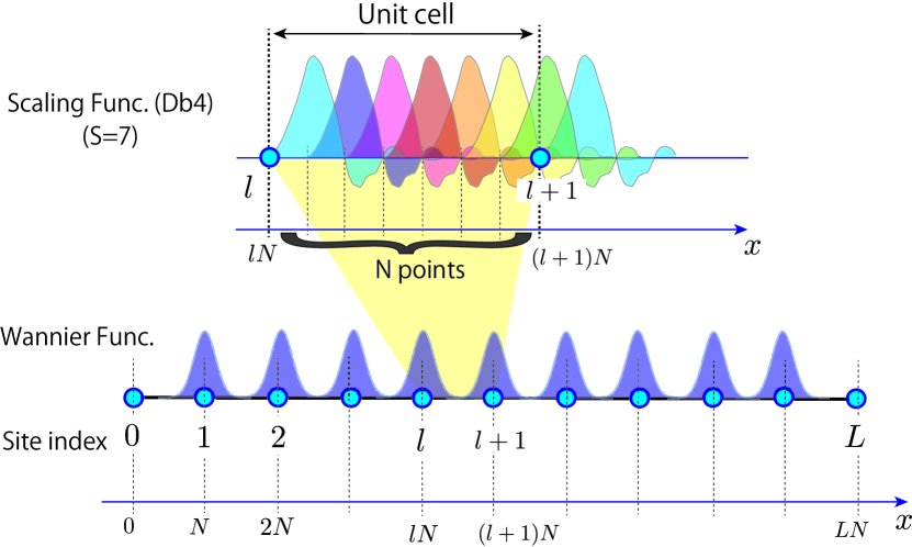
Figure 1: Schematic diagram of an entire crystal depicting an application of compactly supported orthonormal scaling functions to a 1D crystal with periodic boundary condition (lower) and the detail of one unit cell (upper). Cyan circles represent the left edges of unit cells, with which schematic pictures of Wannier functions drawn in grayish blue are associated (lower). Each unit cell is divided in $N$ to assign translationally identical scaling functions colored from blue to green (upper), thereby $LN-1$ of them are deployed over the entire crystal. The scaling functions and the Bloch functions span the identical state space, and hence the Wannier functions shown in the lower figure, as well as the Bloch functions are expressed as linear combinations of the scaling functions.

Meanwhile, the wavelets and scaling functions (SFs)[32] have continuously been developed and applied mostly to signal and image processing [32]. In other areas related to quantum mechanics, Battle applies wavelets to the renormalization group[33], while Evenbly and White built approximations to the ground state of an Ising model by establishing a precise connection between discrete wavelet transforms and entanglement renormalization[34].

In the area of solid state physics related to Wannier functions, Parsen[35], for example, had shown Shannon SF[36], $\mathrm{sinc}(x)$, as a WF in a 1D crystal even before the concept of SF existed. Clow[37] composed a WF from a multi-SF[38] in a similar system. Other than electronic system, phononic[39] and photonic[40] wave functions composed of 2D wavelets are used to calculate band gaps in crystals. This implies SFs are capable of becoming products and ingredients of BFs.

Figure 1 depicts a schematic application of a series of orthonormal SFs[41] to a 1D crystal system. The WFs and the SFs in Fig. 1 resemble each other; they both are translationally orthonormal and localized. Although SFs have a clear mathematical definition[42], they are not eigenfunctions of any observables. This may make SFs as mere means to calculate the results and their physical meaning is hard to conceive. In the paper, the authors attempt to generate position scaling-eigenfunctions, discrete versions of the Dirac’s $\delta$-function, which are SFs and at the same time eigenvectors of an observable. The efficacy of the position eigenvectors projected onto composite band systems, as alternatives to MLWFs, are subsequently examined.

II Composing Position Scaling-Eigenfunction and Computing Matrix Elements of Operators

In this section, position eigenfunctions in a discrete system are generated from known SFs by taking advantage of the two-scale relation, and their properties are studied. Subsequently, the matrix elements of the kinetic energy operator are calculated with the generated position eigenfunctions, since the matrix is used in Sec. V to solve Schrödinger and Maxwell’s equations.

II.1 Overview of Scaling Function

The lower half of Fig. 1 shows $N$ compactly supported SFs deployed in one unit cell to compose BFs and WFs. The SFs in the series have the identical shape, and they are translationally orthonormal, i.e.,

$$\begin{array}[]{c}\int\phi(x-n_{1})\phi(x-n_{2})dx=\delta_{n_{1},n_{2}}\quad(n_{1},n_{2}\in\mathbb{Z}).\\ \end{array}$$ (1)

The particular SFs shown in the Fig. 1 are Daubechies-4s (Db4s). Each of them has nonzero value only inside the continuous region whose width is $7$. Since the continuous region, the support, limits the range of calculations such as integration, compactly supported SFs are particularly useful basis functions when composing and decomposing a function.

While many of the orthonormal sets used in solid state physics are eigenfunctions of Hermitian operators, an SF does not have its origin in physics. They are the solutions of the following recursive algebraic equation called two-scale relation[42]:

$$\begin{split}\phi(x)=\sqrt{2}\sum_{l=0}^{S}h_{l}\phi(2x-l),\\ \{\ h_{l}:0\leq l\leq S,l\in\mathbb{Z},h_{l}\in\mathbb{R}\},\end{split}$$ (2)

with

$$\begin{split}\int\phi(x-n)dx=1\ (n\in\mathbb{Z}).\\ \end{split}$$ (3)

Once the series $\{h_{l}\}$ is given, Eq. (2), the two-scale equation, is recursively solved point-by-point (see Ref. [41] for the specific values of $\{h_{l}\}$ and more sophisticated and detailed treatment of the two-scale relation). Thus, the series $\{h_{l}\}$ determines all characteristics of the corresponding SF.

Figure 2 shows examples of orthonormal compactly supported scaling functions[41], Daubechies-2 to -5 (Db2 to Db5), Symlet-4(Sy4) and Coiflet-1(Cf1), which are created from different sets of $\{h_{l}\}$.

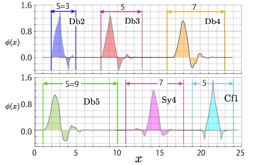
Figure 2: Examples of compactly supported scaling functions and their support lengths $S$. Each compactly supported scaling function has its own support, outside which the value of the scaling function is completely zero. In general, the longer the support is, the smoother the SF becomes.

II.2 Composing Position Eigenfunction

Position eigenvectors in a discrete system not only have to be translationally orthonormal, but also they are desired to be strongly localized and at least twice differentiable. If the space is spanned by a limited number of broad and smooth basis vectors, such as plane waves, strongly localized orbits/position eigenvectors with an exponential decay may not be composed.

The compactly supported SFs, such as Db4s, readily posse some of the rare characters mentioned above. In fact, a compactly supported SF is a good first approximation of the constructed position eigenvector as shown later in Table 1 in Sec. II.2.3. Furthermore, most of them are found to be practically twice differentiable in a sense shown in Appendix A.3 and as demonstrated by the numerical results. Thus, the compactly supported SFs are chosen to be the building blocks of position eigenfunctions.

II.2.1 Strategy

To switch to the Dirac notation, we would like to have the state space representation of an SF such as Db2-Db5, Sy4 and Cf1. Let $|n\rangle$ be the state vector pertaining to an SF, $\phi(x-n)$. Then $|n\rangle$ is formally composed by the position eigenvector $|x\rangle$:

$$|n\rangle=\int dx\phi(x-n)|x\rangle\quad(\;\mathrm{or}\;\;\phi(x-n)=\langle x|n\rangle\;),$$ (4)

where $n$ corresponds to the position of a sub-cell seen in Fig. (1). Therefore, the scaling-kets span the following space:

$$\mathcal{H}_{S}={\mathrm{Span}}\{|n\rangle:n\in\mathbb{Z}\}.$$ (5)

By defining the position operator $\tilde{x}$ in $\mathcal{H}_{S}$:

$$\begin{array}[]{c}\tilde{x}=\hat{P}_{S}\hat{x}\hat{P}_{S},\\ \hat{P}_{S}=\sum_{n}|n\rangle\langle n|,\end{array}$$ (6)

the eigenvectors of the position operator, $\{|x_{p}\rangle\}$, are given as solutions of the following eigenvalue equation:

$$\tilde{x}|x_{p}\rangle=x_{p}|x_{p}\rangle,\ (|x_{p}\rangle\in\mathcal{H}_{S},p\in\mathbb{Z}).$$ (7)

$|x_{p}\rangle$ is expanded by the compactly supported scaling kets:

$$\begin{split}|x_{p}\rangle&=\sum_{n}|n\rangle\langle n|x_{p}\rangle\\ &=\sum_{n}\xi_{n,p}|n\rangle,\end{split}$$ (8)

where

$$\begin{split}\xi_{n,p}=\langle n|x_{p}\rangle.\end{split}$$ (9)

Thus, the unknown to solve is now shifted from the position eigenvectors to the matrix $\{\xi_{n,p}\}$. By multiplying $\langle m|$ from the left to the both sides of Eq. (7):

$$\begin{split}\langle m|\tilde{x}|x_{p}\rangle&=\sum_{n}X_{m,n}\xi_{n,p},\\ \langle m|x_{p}|x_{p}\rangle&=x_{p}\xi_{m,p},\\ \end{split}$$ (10)

where

$$X_{m,n}=\langle m|\tilde{x}|n\rangle.$$ (11)

And hence the equation for $\xi_{m,n}$ is obtained:

$$\sum_{n}X_{m,n}\xi_{n,p}=\xi_{m,p}x_{p}.$$ (12)

II.2.2 Position Operators and Matrix Elements

$\{X_{m,n}\}$ can be obtained from the following integral:

$$\begin{split}X_{m,n}=\int\phi(x-m)x\phi(x-n)dx.\\ \end{split}$$ (13)

Owing to the two-scale relation, Eq. (2), however, the above is recursively expressed by $\{X_{m,n}\}$ without actual integration:

$$\begin{split}\int&\phi(x-m)x\phi(x-n)dx\\ &=\sum_{l,k}2\int h_{l}h_{k}\phi(2x-2m-l)x\phi(2x-2n-k)dx\\ &=\frac{1}{2}\sum_{l,k}h_{l}h_{k}X_{2m+l,2n+k}.\end{split}$$ (14)

By combining Eqs. (13) and (14), we have solvable algebraic equations for $\{X_{m,n}\}$ with given coefficients $\{h_{l}\}$(see Appendix A.1 for the general strategy to calculate matrix elements). Since the support is compact, the integration becomes $0$ for $|m-n|\geq S$. This makes matrix $\{X_{m,n}\}$ sparse and easy to handle. From the translational symmetry, the diagonal elements are simplified to be:

$$\begin{split}X_{m,m}&=\int\phi(x-m)x\phi(x-m)dx\\ &=\int\phi(y)(y+m)\phi(y)dy\quad(y=x-m)\\ &=X_{0,0}+m.\end{split}$$ (15)

By defining the following series $\{X_{r}\}$:

$$X_{r}=\begin{cases}X_{m+r,m}&(\mathrm{for\ }r\neq 0)\\ X_{0,0}&(\mathrm{for\ }r=0),\end{cases}$$ (16)

$X_{m,n}$ is described by $X_{r}$ as follows:

$$X_{m,n}=X_{r}+m\delta_{m,n}\quad(r=m-n).$$ (17)

By substituting this into Eqs. (13) and (14), the following equations for $\{X_{r}\}$ are obtained:

$$\begin{array}[]{l}\bm{X}=\mathbf{H}\bm{X}+\bm{h},\\ \left[\mathbf{H}\right]_{r,q}=\frac{1}{2}\sum_{k}h_{k}h_{k+2r-q},\\ \left[\bm{X}\right]_{q}=X_{q},\\ \left[\bm{h}\right]_{r}=\frac{1}{2}\sum_{k}kh_{k-2r}h_{k}.\end{array}$$ (18)

Since the above equations are linear algebraic and $\{h_{l}\}$ is given, it does not take any actual integration to obtain the matrix elements of the position operator, $\{X_{r}\}$.

Table 8 in Appendix A.2 shows $\{X_{r}\}$ calculated with the listed SFs by numerically solving Eq. (18).

II.2.3 Position eigenvector

Since the shape of the SFs and the position eigenfunctions are translationally invariant, the matrix $\{\xi_{m,n}\}$ is also reduced to a series $\{\xi_{r}\}$:

$$\xi_{m+r,m}\rightarrow\xi_{r},$$ (19)

as detailed in Appendix B.2.1, this simplifies the Eq. (12) to the following equations for $\{\xi_{n}\}$,

$$\begin{split}\sum_{n}\{X_{m-n}\xi_{n-p}+m\delta_{m,n}\xi_{n-p}\}=x_{p}\xi_{m-p}.\end{split}$$ (20)

As described in Appendix B.2.2, Eq. (20) can be solved both analytically and numerically. The central part of the series, $\{\xi_{r}\}$, is shown in Table 1.

Table 1: Central part of the numerical values of of $\{\xi_{p}\}$ corresponding to the SF indicated in the first column. The values are obtained by numerically solving Eq. (20) with GSL library[43].

		$\xi_{-2}$	$\xi_{-1}$	$\xi_{0}$	$\xi_{1}$	$\xi_{2}$
1. SF
a. Sy4		-0.016	-0.023	1.000	0.023	0.017
b. Db2		0.004	-0.070	0.995	0.071	0.001
c. Db3		0.017	-0.119	0.985	0.121	-0.002
d. Db4		0.032	-0.159	0.973	0.165	-0.006

By using Eq. (8) and $\{\xi_{p}\}$, the coordinate representation of the position eigenvector $\xi_{p}(x)$ is obtained:

$$\begin{split}\xi_{p}(x)&=\langle x|x_{p}\rangle\\ &=\sum_{n}\xi_{n,p}\langle x|n\rangle\\ &=\sum_{n}\xi_{n-p}\phi(x-n),\\ \end{split}$$ (21)

where $\phi(x)$ is the given compactly supported SF, such as Db2-Db5 and Sy4.

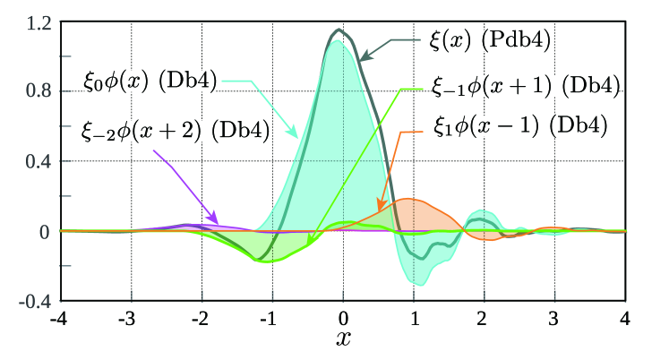
Figure 3: Position eigenfunction $\langle x|\xi_{p=0}\rangle=\xi(x)$ (Pdb4) composed of Db4s. A Pdb4 is drawn with a gray thick line, and its components, Db4s multiplied by $\xi_{r}$, are drawn with colored lines. $\xi_{-1}$ in green adds negative leading part to the central cyan-colored Db4 and the $\xi_{1}$ in pink lifts up the trailing negative part of the central Db4, thereby making the position eigenfunctions more symmetric than the Db4 colored in cyan, which is the main component of the Pdb4.

Fig. 3 shows a position eigenfunction Pdb4 with its component Db4s. It is seen the Pdb4 appears more symmetric than Db4, and the Pdb4 decays exponentially (see Appendix B.2.3). The support appears to be virtually compact, extending approximately from $-3$ to $3$.

Figure 4 shows position eigenfunctions composed of Db2-Db5 (Pdb2-Pdb5), Sy4 (Psy4) and Cf1 (Pcf1). As does the Pdb4 in Fig. 3, Pdb2, Pdb3 and Pdb5 appear to be more symmetric than the corresponding compactly supported SFs. On the other hand, Psy4 and Sy4, Pcf1 and Cf1 look nearly the same, since Sy4 and Cf1 are designed to be more symmetric than Dbns are[41, 44].

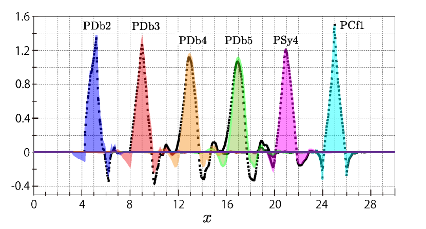
Figure 4: Position eigenfunctions. From left to right, Pdb2, Pdb3, Pdb4, Pdb5, Psy4 and Pcf1. The corresponding SFs are drawn with dashed black lines.

.

Note that the number of basis vectors in $\{|n\rangle\}$ and $\{|x_{n}\rangle\}$ are the same and both sets are orthonormal, and hence they span the identical space:

$$\begin{split}&\mathcal{H}_{X}={\mathrm{Span}}\{|x_{p}\rangle:p\in\mathbb{Z}\},\\ &\mathcal{H}_{S}=\mathcal{H}_{X}.\end{split}$$ (22)

II.2.4 Shifting Eigenfunction and Eigenvalue

The $0$-th eigenvector has $X_{0}$ as its eigenvalue (see Table 8 in Appendix A.2). It is however more convenient to have a direct association of the eigenvector number and the eigenvalue. By shifting the eigenfunctions by $X_{0}$:

$$\xi_{p}(x)\rightarrow\xi_{p}(x+X_{0}),$$ (23)

the transformation from an SF to the position eigenfunction changes as follows:

$$\xi_{p}(x)=\sum_{n}\xi_{n-p}\phi((x+X_{0})-n).$$ (24)

Consequently the eigenvalue is adjusted to be:

$$\tilde{x}|x_{p}\rangle=p|x_{p}\rangle.$$ (25)

II.2.5 Position Eigenvector as Scaling Function

As detailed in Appendix B.2.2, the translational invariance of $\{\xi_{n-m}\}$ leads to the conclusion that the position eigenvectors are also categorized to be SFs. Namely, they themselves satisfy the following two-scale relation:

$$\xi(x)=\sqrt{2}\sum_{l}\eta_{l}\xi(2x-l),\\ \quad\eta_{l}=\sum_{p,q,l}\xi_{p}\xi_{q}h_{q+l-2p}.$$ (26)

The position eigenvectors therefore have their own wavelets, which are shown in Appendix B.3. They may be utilized to solve or analyze quantum mechanical systems where multi-resolution capability are important.

II.3 Computing Matrix Elements of Kinetic Energy Operator

The matrix elements of the kinetic energy operator, $\{P_{r}\}$, are first calculated with a set of compact support SFs without any actual integration or differentiation. Subsequently, $\{P_{r}\}$ are converted to the matrix elements pertaining to the position scaling-eigenvectors, $\{Q_{r}\}$, by using $\{\xi_{r}\}$.

As detailed in Appendix A.3, we have the equations for the matrix elements of $\hat{p}^{n}$:

$$\begin{array}[]{l}\mathbf{K}\cdot\bm{P}=\rho\bm{P},\\ \left[\mathbf{K}\right]_{r,q}=\sum_{k}h_{k}h_{k+2r-q},\\ \begin{aligned} \left[\bm{P}\right]_{r}&=P_{r}\\ &=\langle r|\hat{p}^{n}|0\rangle,\\ \end{aligned}\\ n=\log_{2}\rho.\end{array}$$ (27)

The specific values of $\{P_{r}\}$ obtained from the above equations are listed on Tables 10 and 11. Note that when the eigenvalue $\rho=2$, $\{P_{r}\}$ are the matrix elements of the momentum operator. When $\rho=4$, $\{P_{r}\}$ are the elements of the kinetic energy operator. The reason and the details of solution procedure are detailed in Appendix A.3.

By using $\{\xi_{p}\}$, we get the matrix elements of the kinetic energy operator associated with the position scaling-eigenvectors:

$$\begin{split}Q_{r}&=\langle x_{r}|\hat{p}^{2}/2|x_{0}\rangle\\ &=\sum_{k,l}\{\xi_{k-r}\langle k|\}\hat{p}^{2}/2\{\xi_{l}|l\rangle\}\\ &=\sum_{k,l}\xi_{k-r}\xi_{l}P_{k,l}\\ &=\sum_{k,q}\xi_{k-r}\xi_{k-q}P_{q}.\\ \end{split}$$ (28)

Table 2 shows the numerically obtained $\{Q_{r}\}$.

A measure of differentiability, the Hölder exponents[45] are shown in Table 3 together with the support lengths. Roughly speaking, for instance, Db4 is $1.6179$ times differentiable and other Hölder exponents are also smaller than $2$. The matrix elements of the kinetic energy are nevertheless obtained, and they produce as good results as the preceding ones as shown in Sec. VI. The reason Pdb2 does not have adequate values of the matrix elements are discussed in Appendix A.3.2.

Table 2: Matrix elements of $\hat{p}^{2}/2$, $Q_{r}=\langle x_{r}|\ \hat{p}^{2}/2|x_{0}\rangle$ obtained with different position scaling-eigenfunctions.

		$-Q_{0}$	$-Q_{1}$	$-Q_{2}$	$-Q_{3}$	$-Q_{4}$
1. Position eigenfunction
a. Psy4		-4.008	2.540	-0.671	0.145	-0.010
b. Pdb2
c. Pdb3		-5.265	3.389	-0.876	0.114	0.005
d. Pdb4		-3.991	2.529	-0.668	0.144	-0.010

Table 3: Support lengths and Hölder exponents of SFs.

	Support		Hölder exponent $\alpha$
1. SF
a. Db2	3		0.5500
b. Db3	5		1.0878
c. Db4	7		1.6179
d. Db5	9		1.596
e. Sy4	7
f. Cf4	5

II.4 Adapting Eigenvectors to Crystal System

To apply the position eigenfunctions to 1D electronic and photonic crystals with continuous real coordinates, the following assumptions are made: (1) The periodic boundary condition is imposed at the both ends of the crystal. (2) The unit cell length is set at 1. (3) In electronic systems, the following units are used: $m=1,\;\hbar=1$. (4) In optical systems, the speed of light $c$ is set at 1. (5) The unit cells are divided in $N$ and $\Delta x=1/N$. These assumptions result in the following adjustment to the functions, operators and variables as described in Appendix B.4:

$$\begin{array}[]{c}p\rightarrow x_{p}=l+m\Delta x,\\ Q_{r}\rightarrow N^{2}Q_{r}\quad(\rho=4),\\ \end{array}$$ (29)

with

$$\begin{array}[]{c}\Delta x=1/N,\\ l=p\!\!\!\!\mod N,\\ m=p-lN,\\ \end{array}$$ (30)

and

$$\begin{split}\langle x|x_{p}\rangle&=\sqrt{N}\xi(N(x-x_{p})),\\ \end{split}$$ (31)

$$\begin{split}\int dx\langle x|x_{p}\rangle&=\sqrt{N}\int dx\xi(N(x-x_{p}))\\ &=\sqrt{N}\int\xi(y-p)\frac{dy}{N}\\ &=1/\sqrt{N}.\\ \end{split}$$ (32)

II.5 Single-Band Bloch Functions

A BF pertaining to the $n$-th band with its wave number $k$ has the next form:

$$\begin{split}|\psi_{k}^{n}\rangle&=\frac{1}{\sqrt{L}}e^{ik\tilde{x}}|u_{k}^{n}\rangle.\\ \end{split}$$ (33)

The cell-periodic part $|u_{k}^{n}\rangle$ is expanded by $\{|x_{p}\rangle\}$:

$$\begin{split}|u_{k}^{n}\rangle&=\left\{\sum_{p=0}^{NL-1}|x_{p}\rangle\langle x_{p}|\right\}|u_{k}^{n}\rangle\\ &=\sum_{p=0}^{NL-1}c_{p,k}^{n}|x_{p}\rangle,\\ \end{split}$$ (34)

where $\{c^{n}_{p,k}\}$ is the $N$-periodic (cell-periodic) coefficients of expansion:

$$c^{n}_{p,k}=c_{p+N,k}^{n}=\langle x_{p}|u_{k}^{n}\rangle,$$ (35)

and hence by utilizing Eq. (30):

$$\begin{split}|u_{k}^{n}\rangle&=\sum_{l=0}^{L-1}\sum_{m=0}^{N-1}c_{m,k}^{n}|x_{Nl+m}\rangle\\ &=\sum_{l=0}^{L-1}\sum_{m=0}^{N-1}c_{m,k}^{n}|x_{p}\rangle.\\ \end{split}$$ (36)

The BF is thus decomposed with $\{|x_{p}\rangle\}$:

$$\begin{split}|\psi^{n}_{k}\rangle&=\frac{1}{\sqrt{L}}\sum_{l=0}^{L-1}\sum_{m=0}^{N-1}e^{ik\tilde{x}}c_{m,k}^{n}|x_{p}\rangle\\ &=\frac{1}{\sqrt{L}}\sum_{l=0}^{L-1}\sum_{m=0}^{N-1}e^{ikl}e^{ikm\Delta x}c_{m,k}^{n}|x_{p}\rangle,\end{split}$$ (37)

where Eq. (166) in Appendix B.5.1 is applied.

II.6 State Vectors and Spatial Resolution

In many cases, to solve the Schrödinger equation, it takes discretization of the entire state space $\mathcal{H}$ by a set of a finite number of basis vectors, $\{|\eta_{m}\rangle\}$, which may be plain waves, Gaussian functions, atomic orbits and so on. The position eigenvectors of the discretized space:

$$\mathcal{H}_{\eta}=\mathrm{Span}\{|\eta_{m}\rangle\>,0\leq m<N\},$$ (38)

are obtained by solving the following equation:

$$\begin{split}\tilde{x}|x^{\eta}_{p}\rangle=x^{\eta}_{p}|x^{\eta}_{p}\rangle,\ \left(|x^{\eta}_{p}\rangle=\sum_{m}u^{p}_{m}|\eta_{m}\rangle\right).\end{split}$$ (39)

Then $\xi^{\eta}_{p}(x)=\sqrt{N}\langle x|x^{\eta}_{p}\rangle$ is the discretized version of $\delta$-function in $\mathcal{H}_{\eta}$, and it provides the information on the spatial resolution constrained by $\{|\eta_{m}\rangle\}$.

In this paper, the basis vectors themselves are position eigenvectors and the spatial resolution of the solutions such as BFs and WFs are clear from the time of formulation, as described in Appendix B.5.

III MLWF and Position Scaling-Eigenvector in State Space

The section focuses on the properties of the position eigenvectors projected onto a composite energy band space, $\mathcal{H}_{C}$, consisting of $n_{c}$ energy bands defined as follows:

$$\begin{split}&\mathcal{H}_{C}=\sum_{n}\mathcal{H}_{B_{n}},\\ &\mathcal{H}_{B_{n}}=\mathrm{Span}\{|\psi_{lk_{0}}^{n}\rangle\>\ 0\leq l<L,k_{0}=2\pi/L\},\end{split}$$ (40)

where $L$ is the number of the unit cells in the system and energy bands included in $\mathcal{H}_{C}$ are arbitrary and $n$ does not have to begin from $0$ and the band indexes do not have to be successive numbers.

Subsequently, the relationship between the projected position eigenvectors and MLWFs in $\mathcal{H}_{C}$ leading to approximations of MLWFs by the projected eigenvectors is discussed.

III.1 MLWF

In the section, important properties of MLWFs utilized in the succeeding sections are reviewed in preparation for discussing approximation utilizing the position scaling-eigenvectors,

III.1.1 Eigenvalue Equations for MLWFs

MLWFs satisfy the following equation[24, 25]:

$$\begin{split}\tilde{x}^{C}|W\rangle&=x|W\rangle,\\ \end{split}$$ (41)

where $\tilde{x}^{C}$ is the position operator in $\mathcal{H}_{C}$:

$$\begin{split}\tilde{x}^{C}&=\hat{P}_{C}\hat{x}\hat{P}_{C},\\ \hat{P}_{C}&=\sum_{k,n}|\psi_{k}^{n}\rangle\langle\psi_{k}^{n}|.\end{split}$$ (42)

Because of the number of basis vectors and the translational invariance of the system, the solution has to have the following form (see Appendix C.1):

$$\begin{split}\tilde{x}^{C}|W^{s}_{l}\rangle&=(x_{0s}+l)|W^{s}_{l}\rangle,\\ \end{split}$$ (43)

with

$$\tilde{x}^{C}|W^{s}_{0}\rangle=x_{0s}|W^{s}_{0}\rangle,$$ (44)

where $s$ and $l$ denote the series and the cell number, respectively. The number of series is $n_{c}$, for the number of energy bands involved is $n_{c}$.

The MLWF as a function of position is given by the following projection (see Appendix C.2):

$$\begin{split}\langle x_{p}|W^{s}_{l}\rangle&=N^{-1/2}W^{s}_{0}(x_{p}-l)\\ &=N^{-1/2}W^{s}_{l}(x_{p}).\end{split}$$ (45)

III.1.2 Orthonormality of MLWFs

Because MLWFs have to be orthonormal:

$$\begin{split}\langle W^{s_{1}}_{l_{1}}|W^{s_{2}}_{l_{2}}\rangle=\delta_{s_{1},s_{2}}\delta_{l_{1},l_{2}}.\\ \end{split}$$ (46)

The numbers of MLWFs and BFs are the same, and they span the same space, $\mathcal{H}_{C}$ and hence:

$$\hat{P}_{C}=\sum_{l,s}|W_{l}^{s}\rangle\langle W_{l}^{s}|=\sum_{k,n}|\psi_{k}^{n}\rangle\langle\psi_{k}^{n}|.$$ (47)

Since MLWFs are expanded as described in Appendix C.1:

$$|W_{l}^{s}\rangle=\sum_{k}e^{-ikl}w_{k}^{s,n}|\psi_{k}^{n}\rangle,$$ (48)

the following holds:

$$\langle W_{l_{1}}^{s_{1}}|W_{l_{2}}^{s_{2}}\rangle=\sum_{k}e^{-ik(l_{2}-l_{1})}\sum_{n}\left(\overline{w}_{k}^{s_{1},n}w_{k}^{s_{2},n}\right).$$ (49)

Throughout the paper overline on a variable, such as $\overline{\square}$, denotes the complex conjugate of the variable underneath.

By the requirement given by Eq. (46) for any $l_{1},l_{2}\in\mathbb{Z}$, we have:

$$\sum_{n}\overline{w}_{k}^{s_{1},n}w_{k}^{s_{2},n}=\frac{1}{L}\delta_{s_{1},s_{2}}.$$ (50)

III.2 Position Eigenvectors Projected onto Composite Band Space

The section focuses on the properties of the position eigenvectors when they are projected onto composite bands.

III.2.1 Definition

MLWFs are the eigenvectors of the operator that is the position operator projected onto $\mathcal{H}_{C}$, as described in Eq. (42). In contrast to this, the projected position eigenvectors (PPE) are defined as the position eigenvectors, $|x_{p}\rangle\in\mathcal{H}_{X}$, projected onto $\mathcal{H}_{C}$:

$$\begin{split}|x^{C}_{p}\rangle&=\hat{P}_{C}|x_{p}\rangle\\ &=\sum_{k,n}\!|\psi^{n}_{k}\rangle\langle\psi^{n}_{k}|x_{p}\rangle\\ &=\frac{1}{\sqrt{L}}\sum_{k,n}e^{-ikl}e^{-ikm\Delta x}\bar{c}^{n}_{m,k}|\psi^{n}_{k}\rangle,\end{split}$$ (51)

where the superscript $C$ denotes that the vector is not a position eigenvector in $\mathcal{H}_{X}$, but in $\mathcal{H}_{C}$.

III.2.2 Properties of PPE

Since any vector in $\mathcal{H}_{C}$ is expanded by $|\psi^{n}_{k}\rangle\in\mathcal{H}_{C}$:

$$|f\rangle=\sum_{n,k}f^{n}_{k}|\psi^{n}_{k}\rangle.$$ (52)

The projection of $|f\rangle$ onto a PPE becomes:

$$\begin{split}\langle x^{C}_{p}|f\rangle&=\left\{\langle x_{p}|\sum_{n_{1},k_{1}}|\psi^{n_{1}}_{k_{1}}\rangle\langle\psi^{n_{1}}_{k_{1}}|\right\}\sum_{n,k}f^{n}_{k}|\psi^{n}_{k}\rangle\\ &=\sum_{n,k}\langle x_{p}|\psi^{n}_{k}\rangle f^{n}_{k}\\ &=\langle x_{p}|f\rangle,\end{split}$$ (53)

and hence PPEs behave as if they were the position eigenvectors in $\mathcal{H}_{C}$.

It is also noted that the inner product is a measure of closeness of the two vectors and by definition:

$$\cos\theta_{x_{p},f}=\langle x^{C}_{p}|f\rangle/\sqrt{\langle x^{C}_{p}|x^{C}_{p}\rangle\langle f|f\rangle}.$$ (54)

From Eq. (167) in Appendix B.5.2,

$$\langle x_{p}|f\rangle=\frac{1}{\sqrt{N}}(f(x_{p})+O(\sigma_{0}^{2}/N^{2})),$$ (55)

the value of a function at $x=x_{p}$ is a measure of the closeness between the vector and the corresponding PPE.

III.2.3 Approximation of PPE

By utilizing Eq. (55),

$$\langle\psi^{n}_{k}|x_{p}\rangle\simeq\frac{\overline{\psi}^{n}_{k}(x_{p})}{\sqrt{N}}.$$ (56)

PPE defined by Eq. (51) is therefore approximated with the values of the BFs pointwise:

$$|\tilde{x}^{C}_{p}\rangle=\sum_{k,n}\frac{\overline{\psi}^{n}_{k}(x_{p})}{\sqrt{N}}|\psi_{k}^{n}\rangle,$$ (57)

which is calculated from the values of the BFs rather than $\{c^{n}_{pk}\}$. From Eq. (167), the error is given as follows:

$$\langle x|x^{C}_{p}\rangle=\langle x_{p}|\tilde{x}^{C}_{p}\rangle+O(\sigma_{0}^{2}/N^{2}).$$ (58)

To distinguish $|\tilde{x}^{C}_{p}\rangle$ from PPE, it is termed pointwise projected position eigenvector (PWE).

III.3 Approximation of MLWF with PPE

The section describes the following properties of PPEs and PWEs in relation to MLWFs to examine the possibility of PPEs and PWEs being used as alternatives or supplements to MLWFs: (1) Closeness in terms of shape and position. (2) Closeness in terms of their characters in the relevant space, i.e., intra- and inter-series orthonormality.

The results of the analysis justify the intuitive closeness of PPEs and PWEs to MLWFs. The similarities and differences are summarized in Appendix C.5. Furthermore, it is shown that a relatively light calculation, searching the maximum point of a function, $F(m)=\sum_{k}\left|c_{m,k}\right|^{2}$, gives the maximum point of the MLWF.

The specific estimate of error associated with the approximation of an MLWF by the PPE will be presented later in Sec. IV.2.2, albeit, for single band cases.

III.3.1 Maximum Point of PPE and MLWF

When $|x_{p}^{C}\rangle$ is closest to $|W^{s}_{l}\rangle$ among:

$$\{|x^{C}_{q}\rangle:0\leq q<NL\},$$ (59)

$x_{p}$ is the maximum point of $\left|W_{l}(x)\right|$ from Eqs. (45) and (54). Combining the above and the following equation obtained in Appendix C.4.1:

$$\begin{split}\xi_{p}^{C}(x)=\langle x|x_{p}^{C}\rangle&\simeq N^{-1/2}W^{s}_{l}(x)\overline{W}^{s}_{l}(x_{p}),\end{split}$$ (60)

we notice the position $x_{p}$ is also the maximum point of $\xi^{C}_{p}(x)$. Thus, finding the maximum point of an MLWF is achieved by searching the maximum point of the tallest PPE. It should be however noted, in cases PPEs do not have a clear maximum, as will be shown later in Sec. V.3 (e.g.,Fig. 11(d)), the actual $\sigma^{2}_{x}$ (spread) has to be calculated to identify the maximally localized PPE.

To signify the difference between PPE and PWE, and to show the procedure of finding the approximate position of an MLWF to a programmable degree, the section focuses on the single band case. By restricting the band index to $n$, a PPE projected onto itself is calculated as follows:

$$\begin{split}\xi_{p}^{n}(x_{p})&=\langle x^{n}_{p}|x_{p}^{n}\rangle\\ &=\sum_{k}\langle x_{p}|\psi^{n}_{k}\rangle\langle\psi^{n}_{k}|x_{p}\rangle\\ &=\sum_{k,p_{1},p_{2}}\langle x_{p}|\left\{\frac{1}{\sqrt{L}}e^{ikx_{p_{1}}}c^{n}_{p_{1},k}|x_{p_{1}}\rangle\right\}\\ &\quad\quad\quad\quad\quad\left\{\frac{1}{\sqrt{L}}\langle x_{p_{2}}|e^{-ikx_{p_{2}}}\overline{c}^{n}_{p_{2},k}\right\}|x_{p}\rangle\\ &=\sum_{k}\left|c^{n}_{p,k}\right|^{2},\end{split}$$ (61)

with

$$\begin{split}m=p\ \mathrm{mod}\ N,x_{p}=p\Delta x.\end{split}$$ (62)

On the other hand, a PWE projected onto itself is calculated as follows:

$$\begin{split}&\ \langle\tilde{x}_{p}^{n}|\tilde{x}_{p}^{n}\rangle=\frac{1}{N}\sum_{k_{1},k}\left\{\langle\psi_{k_{1}}^{n}|\psi^{n}_{k_{1}}(x_{p})\right\}\left\{\overline{\psi}_{k}^{n}(x_{p})|\psi^{n}_{k}\rangle\right\}\\ &\quad\quad\quad=\frac{1}{N}\sum_{k}\psi_{k}^{n}(x_{p})\overline{\psi}_{k}^{n}(x_{p})\\ &\ \quad\quad\left(=\sum_{k}\left|c_{p,k}^{n}\right|^{2}+O\left(\sigma^{2}/N^{2}\right)\right),\end{split}$$ (63)

where Eq. (167) in Appendix B.5.1 is utilized.

From the above, the following points are easily understood: (1) Finding the approximate position of the MLWF in a unit cell is reduced to searching the maximum point of $F(m)=\sum_{k}\left|c_{m,k}\right|^{2}$. This is expected to be a relatively light work on computer. (2) PWEs are potentially useful, for it can be computed from known values of the BFs calculated in some other ways.

However, it has to be noted: (a) A PPE and the corresponding PWE are not identical. (b) The spatial resolution is limited by the number of the independent bases vectors used in the calculation of BFs. (c) The distinctiveness of the peak of the PWE depends on the nature of the basis as is mentioned in the opening of Sec. II.2.

III.3.2 Maximum Values of PPE and MLWF

By normalizing the PPE closest to an MLWF, we have the following approximation:

$$|W_{l}^{s}\rangle\simeq\frac{1}{\sqrt{\left|\langle x^{C}_{p}|x^{C}_{p}\rangle\right|}}|x^{C}_{p}\rangle.$$ (64)

By combining the above and Eq. (45), we have:

$$|{W}^{s}_{l}(x_{p})|=\sqrt{N\left|\langle x^{C}_{p}|x^{C}_{p}\rangle\right|}.$$ (65)

Thus, the maximum value of an MLWF is obtained from that of the tallest PPE.

III.3.3 Intra-Series Orthonormalization of PPEs

Since the PPEs defined and described so far are not translationally orthonormal within a series, i.e.:

$$\langle x^{C}|(x+l)^{C}\rangle=N^{-1}\sum_{k,n}\psi^{n}_{k}(x)\overline{\psi}^{n}_{k}(x+l).$$ (66)

To use PPEs as an alternative to MLWFs, they have to be orthonormalized (Appendix C.3), and hence PPEs is redefined as follows:

$$\begin{split}|x^{\perp C}_{p}\rangle&=\sum_{k,n}\frac{1}{\Phi_{k}}\left\{|\psi^{n}_{k}\rangle\langle\psi^{n}_{k}|x_{p}\rangle\right\},\\ \Phi_{k}&=\sqrt{\sum_{n}|\langle\psi^{n}_{k}|x_{p}\rangle|^{2}}.\end{split}$$ (67)

The above definition differs from that of Eq. (51), for $\Phi_{k}$ is at the denominator. However, when $|x^{C}_{p}\rangle$ is closest to an MLWF, from Eq. (198) in Appendix C.4.2, the following holds:

$$\begin{split}\Phi_{k}\simeq\sqrt{\left|\langle x^{C}_{p}|x^{C}_{p}\rangle\right|}.\end{split}$$ (68)

And hence:

$$\begin{split}|x^{\perp C}_{p}\rangle&\simeq\frac{1}{\sqrt{\left|\langle x^{C}_{p}|x^{C}_{p}\rangle\right|}}|x^{C}_{p}\rangle.\end{split}$$ (69)

Therefore, the orthonormalized PPEs are equal to the approximated MLWFS seen in Eq. (64).

Similarly, orthonormalized PWEs are defined as follows:

$$\begin{split}|\tilde{x}^{\perp C}_{p}\rangle&=\sum_{k,n}\frac{\psi^{n}_{k}(x_{p})}{\tilde{\Phi}_{k}}|\psi^{n}_{k}\rangle,\\ \tilde{\Phi}_{k}&=\sqrt{\sum_{n}|\psi^{n}_{k}(x_{p})|^{2}}.\end{split}$$ (70)

III.3.4 Inter-Series Orthonormalization of PPEs

When there are two or more series of MLWFs, the same number of PPE series have to exist, and one series has to be orthogonal to others. Let $|x^{C}_{p_{1}}\rangle$ be the closest PPE to an MLWF in series $s_{1}$, and $x_{p_{0}}$ be the zero of $\xi^{C}_{p_{1}}(x)=N^{-1/2}\langle x|x^{C}_{p_{1}}\rangle$ then

$$\begin{split}|\xi_{p_{1}}(x_{p_{0}})|&=N^{-1/2}|\langle x^{C}_{p_{0}}|x^{C}_{p_{1}}\rangle|\\ &=N^{-1/2}|\langle x^{C}_{p_{1}}|x^{C}_{p_{0}}\rangle|=|\xi_{p_{0}}(x_{p_{1}})|=0.\end{split}$$ (71)

We find $|x^{C}_{p_{1}}\rangle$ and $|x^{C}_{p_{0}}\rangle$ are orthogonal. Thus, an approximation of another series is obtained (see Fig. 14 for example). One unresolved problem is it does not guarantee that $|x^{C}_{p_{0}}\rangle$ is the most localized PPE in the vicinity of $x_{p_{0}}$. Likewise, if $x_{p_{0}}$ is chosen so that $|x^{C}_{p_{0}}\rangle$ is most localized in the vicinity, the inter-series orthogonality is not guaranteed. Nonetheless, the numerical results shown in Sec. VI well agree with MLWFs at least on the figures.

III.4 Density Matrix and Initial-Guess Orbit

Position representation of $\hat{P}_{C}$, the density matrix[28],

$$\begin{split}&\rho_{x_{2}}(x_{1})=\langle x_{1}|\hat{P}_{C}|x_{2}\rangle\\ &\left(|x_{n}\rangle\in\mathcal{H},\ \langle x|x_{n}\rangle=\delta(x-x_{n})\ ,n=1,\ 2\right),\end{split}$$ (72)

is proved to fall off exponentially as a function of $x_{1}$ [10, 21, 48, 49, 50], and it is used as an initial-guess of the MV method either as it is [29, 28, 26, 27] or by replacing the $|x_{2}\rangle$ with a localized wave function such as an atomic orbit expected to be close to the MLWF[30, 8, 31, 19, 28, 6, 29]. The position representation of PPE defined by Eq. (51) and $\langle x^{C}_{p}|f\rangle$ in Eq. (55) resemble the density matrix. In the continuous limit, they are identical, however $|x_{p}\rangle$ and $|f\rangle$ in the paper are vectors in a discretized space $\mathcal{H}_{X}$.

When the state space is spanned by a finite number of orthonormal vectors $\{|\eta_{m}\rangle\}$, as in the case of numerical simulations or mathematical modeling, the state space is discretized as discussed in Sec. II.6:

$$\begin{split}\mathcal{H}&\rightarrow\mathcal{H}_{\eta},\\ \int dx|x\rangle\langle x|&\rightarrow\sum_{m}|\eta_{m}\rangle\langle\eta_{m}|\\ &=\sum_{p}|x^{\eta}_{p}\rangle\langle x^{\eta}_{p}|,\\ \end{split}$$ (73)

where $\{|x^{\eta}_{p}\rangle\}$ is the set of position eigenvectors in $\mathcal{H}_{\eta}$ and spans the same space:

$$\mathrm{Span}\{|x^{\eta}_{p}\rangle\}=\mathrm{Span}\{|\eta_{m}\rangle\}=\mathcal{H}_{\eta}.$$ (74)

And hence the density matrix becomes:

$$\begin{split}\langle x|\sum_{p}|x^{\eta}_{p}\rangle\langle x^{\eta}_{p}|x_{2}\rangle=&N^{-1/2}\langle x|\sum_{p}|x^{\eta}_{p}\rangle\bar{\xi}^{\eta}_{p}(x_{2})\\ =&N^{-1}\sum_{p}\xi^{\eta}_{p}(x)\bar{\xi}^{\eta}_{p}(x_{2}).\end{split}$$ (75)

The right-hand side of Eq. (75) involves more than one position eigenvectors, thereby making the density matrix potentially broader than the inherent spread of $|x^{\eta}_{p}\rangle$ (one example is a delta function overlapping all molecular orbits).

On the other hand, the PPE for $|x_{p_{2}}\rangle\in\mathcal{H}_{x}$ is:

$$\begin{split}\langle x|\sum_{p}|x_{p}\rangle\langle x_{p}|x_{p_{2}}\rangle=&\langle x|\sum_{p}|x_{p}\rangle\delta_{p,p_{p_{2}}}\\ =&N^{-1/2}\xi_{p_{2}}(x).\end{split}$$ (76)

The right-hand side of the above equation consists of only one position eigenfunction.

In the case of the position scaling-eigenfunction, Pdb3, Pdb4, Pdb5 and Psy4, the spreads increase by 10 to 50 % by replacing $|x_{p}\rangle\in\mathcal{H}_{X}$ with $|x_{2}\rangle\in\mathcal{H}$.

IV MLWF and PPE in k-Space

Partial differential equations for MLWFs in k-space give insight into properties of MLWFs and their relatives. The focus of the section is on a description of the degree of the closeness of MLWFs and PPEs, namely Eq. (64).

IV.1 Partial Differential Equations for MLWFs

By expanding MLWFs with the BFs, another solution procedure for MLWFs is obtained:

$$\begin{split}|W\rangle=\sum_{k}\sum_{n}w_{k}^{n}|\psi_{k}^{n}\rangle,\end{split}$$ (77)

where the series number $s$ is dropped and the home unit cell index $l$ is assumed to be $0$. After projecting the Eq. (41) onto the bra of a BF, we have a set of partial differential equations for $w_{k}$ (see Appendix C.6 for the detail):

$$\frac{\partial w_{k}^{n_{1}}}{\partial k}=\sum_{m,n_{2}}\frac{\partial\bar{c}_{m,k}^{n_{1}}}{\partial k}c_{m,k}^{n_{2}}w_{k}^{n_{2}}-ix_{0}w_{k}^{n_{1}},\\$$ (78)

where $x_{0}$ has to be chosen to have maximum localization.

When all energy bands are included in the calculation of MLWFs, the following holds:

$$\mathcal{H}_{C}=\mathcal{H}_{B}=\sum_{n=0}^{N-1}\mathcal{H}_{B_{n}}\\ =\mathcal{H}_{X}.$$ (79)

Therefore, position eigenvectors $\{|x_{p}\rangle\}$, MLWFs and PPEs are identical. In fact, the position eigenvectors can conversely be expanded by the BFs:

$$\begin{split}|x_{p}\rangle&=\sum_{k}\sum_{n=0}^{N-1}|\psi_{k}^{n}\rangle\langle\psi_{k}^{n}|x_{p}\rangle\\ &=\frac{1}{\sqrt{L}}\sum_{k}\sum_{n=0}^{N-1}e^{-ikp\Delta x}\overline{c}_{m}^{n,k}|\psi_{k}^{n}\rangle,\\ \end{split}$$ (80)

and it is easily checked the following satisfies Eq. (78):

$$\begin{split}&w_{k,p}=e^{-ikx_{p}}\overline{c}_{m}^{n,k},\\ &x_{0}=p\Delta x=x_{p}.\end{split}$$ (81)

IV.2 MLWF and PPE in Single-Band System

IV.2.1 Phase of MLWF

When an MLWF’s home unit cell is $[0:1)$, Eq. (78) for single-band system is simplified:

$$\begin{split}\frac{\partial w_{k}}{\partial k}&=\sum_{m}\frac{\partial\bar{c}_{m,k}}{\partial k}c_{m,k}w_{k}-ix_{0}w_{k}.\\ \end{split}$$ (82)

By defining $r_{m,k}$ and $\theta_{m,k}$ in the following way:

$$c_{m,k}=r_{m,k}e^{i\theta_{m,k}},\;r_{m,k},\in\mathbb{R}^{+},\;\theta_{m,k}\in\mathbb{R},$$ (83)

the first term on the right-hand side of Eq. (82) turns out to be the cell expectation value of the change in $\theta_{m,k}$:

$$\begin{split}\sum_{m=0}^{N-1}\frac{\partial\bar{c}_{m,k}}{\partial k}c_{m,k}&=\sum_{m=0}^{N-1}\frac{\partial r_{m,k}e^{-i\theta_{m,k}}}{\partial k}r_{m,k}e^{i\theta_{m,k}}\\ &=-i\sum_{m=0}^{N-1}\frac{\partial\theta_{m,k}}{\partial k}r_{m,k}^{2}.\\ \end{split}$$ (84)

By defining:

$$\bar{\theta}_{k}=\int^{k}dk_{1}\langle\frac{\partial\theta_{k_{1}}}{\partial k_{1}}\rangle_{cell}=\int^{k}dk_{1}\sum_{m=0}^{N-1}\frac{\partial\theta_{m,k_{1}}}{\partial k_{1}}r_{m,k_{1}}^{2},$$ (85)

and choosing $x_{0}$ to make the WF most localized, the MLWF is solved as follows:

$$\begin{split}|W_{l}\rangle&=\sum_{k}e^{-i\bar{\theta}_{k}}e^{-ikx_{0}}e^{-ikl}|\psi_{k}\rangle.\\ \end{split}$$ (86)

In the above equation, the term $e^{-i\bar{\theta}_{k}}$ works to reshape the resulting WF sharper, by making the expectation value of the phase zero at each wave number.

IV.2.2 The Most Localized PPE and Its Error

A PPE in $\mathcal{H}_{B_{1}}$ is:

$$\begin{split}\sum_{k}\!\!|\psi_{k}\rangle\langle\psi_{k}|x_{p}\rangle&\!=\!\frac{1}{\sqrt{L}}\sum e^{-ikl}e^{-ikm\Delta x}\bar{c}_{m,k}|\psi_{k}\rangle.\\ \end{split}$$ (87)

By applying the procedure described in Sec. III.3.3, we have orthonormalized PPE:

$$\begin{split}|x^{\perp}_{p}\rangle&=\frac{1}{\sqrt{L}}\sum_{k}e^{-ikl}e^{-ikm\Delta x}\frac{\bar{c}_{m,k}}{|c_{m,k}|}|\psi_{k}\rangle\\ &=\frac{1}{\sqrt{L}}\sum_{k}e^{-ikl}e^{-ikm\Delta x}e^{-i\theta_{m,k}}|\psi_{k}\rangle\\ &=\sum_{k}b_{p,k}|\psi_{k}\rangle.\end{split}$$ (88)

Thus, the series $\{b_{p,k}\}$ satisfies the following equation:

$$\frac{\partial b_{p,k}}{\partial k}=-i\frac{\partial\theta_{m,k}}{\partial k}b_{p,k}-i(l+m\Delta x)b_{p,k}.$$ (89)

$\bar{c}_{m,k}$ in Eq. (88) offsets the phase of each BF $k$-by-$k$ at $x=p\Delta x=l+m\Delta x$, so that all BFs are aligned at this position.

One of the possible first approximation of Eq. (85), is to replace the expectation values of the phases with the phases at maximum point of the following probability density:

$$\sum_{k}\left|c^{n}_{m,k}\right|^{2}=\sum_{k}\left|r_{m,k}\right|^{2}.$$ (90)

And hence,

$$\begin{split}\int^{k}dk_{1}\sum_{m=0}^{N-1}\frac{\partial\theta_{m,k_{1}}}{\partial k_{1}}r_{m,k_{1}}^{2}&\simeq\sum_{m=0}^{N-1}\theta_{m,k}r_{m,k}^{2}\\ &\sim\theta_{m_{0},k},\\ \end{split}$$ (91)

where $m_{0}$ is the maximum point of Eq. (90).

For the reason, PPEs and MLWFs are close to each other when they are highly localized. And the measure of the error $\delta_{k}$ is:

$$\delta_{k}=|\overline{\theta}_{k}-\theta_{m_{0},k}|.$$ (92)

The above analysis does not directly apply in the case of composite band systems, and still the analysis needs more development. In the paper, the numerical results supporting the validity of the PPE will be shown later in Sec. VI.

V Numerical Scheme

The section describes solution procedures of the 1D Schrödinger and Maxwell’s equations. Especially, the capability of the position scaling-eigenfunctions to diagonalize the potential energy and the electric susceptibility is explained and utilized.

V.1 Diagonalization of Potential Energy and Electric Susceptibility

Since the position scaling-eigenfunctions are chosen as the basis vectors, the position operator $\tilde{x}\in\mathcal{H}_{X}$ is diagonal by definition. And if $V(x)$ is piecewise quadratic over a few calculation cells, as described in detail in Appendix B.5.3, the following holds:

$$\begin{split}\langle x_{p_{1}}|V(\hat{x})|x_{p_{2}}\rangle=V(x_{p_{2}})\delta_{p_{1},{p_{2}}}+O(\sigma^{2}_{0}/N^{2}),\end{split}$$ (93)

where

$$\begin{array}[]{c}\sigma^{2}_{0}=\langle x_{0}|\hat{x}^{2}|x_{0}\rangle,\\ p_{1},p_{2}\in\mathbb{Z}.\end{array}$$ (94)

Since $\sigma^{2}_{0}$ is of the order of $0.1$, the error above is estimated to be $\sim 0.1/N$ and practically negligible. Thus, the potential energy and the electric susceptibility become diagonal with respect to the position scaling-eigenfunctions.

When $V(x)$ is given as a $\delta$-function such as:

$$\begin{split}V(x,a)&=V_{0}\delta(x-a),\end{split}$$ (95)

the corresponding potential energy operator is discretized to be (see Appendix B.5.3 for detail):

$$\begin{split}\hat{V}(a)=NV_{0}|x_{p}\rangle\langle x_{p}|\quad(x_{p}=a,p=a/\Delta x).\end{split}$$ (96)

Thus, the numerical expression of the matrix is diagonal:

$$\begin{split}\langle x_{p_{1}}|\hat{V}(a)|x_{p_{2}}\rangle=V_{0}N\delta_{p_{1},p_{2}}.\end{split}$$ (97)

V.2 Electronic System

Owing to Eq. (171), the operators of the discretized Hamiltonian in $\mathcal{H}_{X}$ becomes:

$$\begin{split}\hat{H}(\hat{p}^{2},\hat{x})\rightarrow\tilde{H}(\tilde{p}^{2},\tilde{x}).\end{split}$$ (98)

By this, the potential energy matrix becomes diagonal if the operator is composed of $\hat{x}$ alone. Thus, the Schrödinger equation becomes:

$$\tilde{H}|\psi^{n}_{k}\rangle=E_{k}^{n}|\psi^{n}_{k}\rangle.$$ (99)

By multiplying the ket of a position eigenvector and substituting Eq. (37) into Eq. (99), we have:

$$\begin{split}\sum_{m_{2}=0}^{N-1}\langle x_{m_{1}}|H|x_{m_{2}}\rangle e^{ik(m_{2}-m_{1})\Delta x}c^{n,k}_{m_{2}}=E_{k}^{n}c^{n,k}_{m_{1}},\\ \langle x_{m_{1}}|H|x_{m_{2}}\rangle=\frac{1}{2}\langle x_{m_{1}}|\hat{p}^{2}|x_{m_{2}}\rangle+v(x_{m_{1}})\delta_{m_{1,}m_{2}}.\end{split}$$ (100)

With the kinetic energy matrix elements, $\{Q_{r}\}$, listed on Table 2, the final form of the eigenvalue equation to determine the series $\{c_{m}^{n,k}\}$ is obtained as follows:

$$\begin{split}\sum_{m_{2}=0}^{N-1}\left[Q_{m_{1}-m_{2}}+\delta_{m_{1},m_{2}}V(m_{2}\Delta x)\right]&e^{ik(m_{2}-m_{1})\Delta x}c_{m_{2}}^{n,k}\\ =&E_{k}^{n}c_{m_{1}}^{n,k}.\end{split}$$ (101)

V.3 Optical System

The equations for the electric field $f(x)$ and magnetic field $h(x)$ satisfy the following equations[51]:

$$\begin{split}-\frac{\partial^{2}}{\partial x^{2}}f(x)&=\left(\frac{\omega}{c}\right)^{2}\epsilon(x)f(x),\\ h(x)&=-\frac{c}{\omega}\frac{\partial}{\partial x}f(x),\end{split}$$ (102)

where $\epsilon(x)\geq 0$ is the dielectric susceptibility function.

By using the same strategy described in Sec. V.2, the discretized equation for the electric field becomes:

$$\begin{split}\sum_{m_{2}=0}^{N-1}Q_{m_{1}-m_{2}}&e^{ik(m_{2}-m_{1})\Delta x}c_{m_{2}}^{n,k}\\ &=\omega^{2}_{k}\epsilon(m_{1}\Delta x)c_{m_{1}}^{n,k}.\end{split}$$ (103)

The set of eigenvalue equations are solved with a math library such as the GSL [43].

V.4 Basis Vectors and BFs

The solutions of Eqs. (101) and (103), $\{c_{k,m}^{n}\}$ are elements of a matrix $\bm{c}_{k}$ transforming the position scaling-eigenvectors $\{|x_{m}\rangle\}$ to the BFs $\{|\psi^{k}_{n}\rangle\}$ and the matrix is inherently square with respect to $m$ (position) and $n$ (energy band). It is noted even if we replace the position scaling-eigenvectors with other basis set, the number of the independent basis vectors in a unit cell and the number of the computable bands are identical.

VI Results and Discussions

The section compares orthonormalized PPEs defined by Eq. (67), orthonormalized PWEs defined by Eq. (70) and MLWFs obtained from Eq. (186) with preceding results.

As the position scaling-eigenfunction, Psy4 is used. Replacing Psy4 with Pdb3, Pdb4 and Pdb5 results in no discernible difference except minor numerical deviation.

Throughout the section, the units of the vertical and horizontal axis are adjusted to the figures in the references, for convenience in comparison, and hence units differ from figure to figure.

VI.1 Numerical Verification of Energy Eigenvalues

To verify the obtained position eigenvectors and the numerical scheme developed in the paper, the electronic and optical energy eigenvalues calculated by Eqs. (101) and (103) are compared with the preceding results. The agreements are quite good, and hence MLWF, PPE and PWE produced by the scheme deserve to be discussed.

VI.1.1 Electronic System

Figure 5 shows two energy band diagrams produced from the method described in Sec. V.2. The calculation conditions are listed in Table 4. Both show good agreements with the preceding results.

Table 4: Units and potential energy employed in the calculation of energy band diagrams shown in Figs. 5(a) and (b).

		Fig. 5(a)	Fig. 5(b)
1. Units
a. Energy		$\hbar^{2}/(2ma_{B}^{2})$	$\hbar^{2}/(2ma^{2})$
b. Length		$a=5a_{B}$	$a=$Unit Cell Size
2. Potential energy
a. $V(x)$		$V_{0}\left[1-\cos\frac{2\pi x}{a}\right]$	$\sum_{n}V_{0}\delta(x-na)$
b. $V_{0}$		$10(\hbar^{2}/2m)(\pi/a)^{2}$	$6\hbar^{2}/(2ma)$

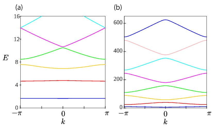
Figure 5: Calculated electronic band structures, where $N=40$, $L=40$. (a) $V(x)=V_{0}\left[1-\cos({2\pi x}/{a})\right]$ [52] (b) $V(x)=\sum_{n}V_{0}\delta(x-na)$ [53].

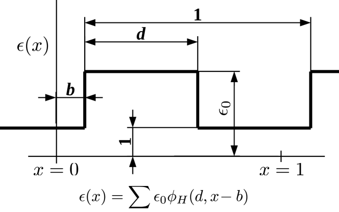
Figure 6: Parameters of dielectric susceptibility $\epsilon(x)$.

VI.1.2 Photonic Systems

The two dispersion diagrams shown in Fig. 7 are calculated from the method described in Sec. V.3. The dielectric susceptibility $\epsilon(x)$, in both cases, is a sort of step functions that is shown in the Fig. 6. The calculation conditions and parameters are shown in Table 5. Both figures well agree with the preceding results.

Table 5: Units and parameters for electric susceptibility $\epsilon(x)$ employed in the calculation of the dispersion diagrams and Wannier functions shown in Figs. 7, 10, 11 and 12. The parameters $\epsilon_{0}$, $b$ and $d$ are defined in the Fig. (6).

		Figs. 7(a), 11 and 12		Figs. 7(b) and 10
1. Units
a. Frequency		$2\pi c$		$c$
b. Length		$a=$Unit Cell Size		$a=$Unit Cell Size
2. Parameters
a. $\epsilon_{0}$		12		5
b. $b$		$0$		$0.35$
c. $d$		$0.5$		$0.3$

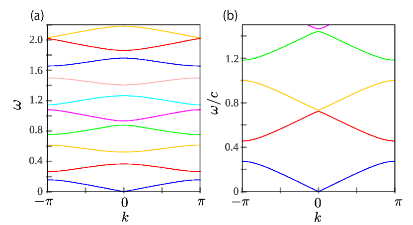
Figure 7: Calculated photonic band structures, where $N=40$, $L=40$. (a) $\epsilon(x)=\sum 12\phi_{H}(1/2,x-n)$ [15]. (b) $\epsilon(x)=\sum 5\phi_{H}(0.3,x-0.35-n)$ [51].

VI.2 WFs in Single Band Systems

The MLWFs, PPEs and PWEs pertaining to $n_{b}$-th energy band are qualitatively and quantitatively compared with preceding results.

VI.2.1 Electronic Systems

The potential energy employed in the cases of Fig. 8, is of Krönig-Penny type as noted in the captions and the MLWF, PPE and PWE well agree with the preceding results[54] in each energy band.

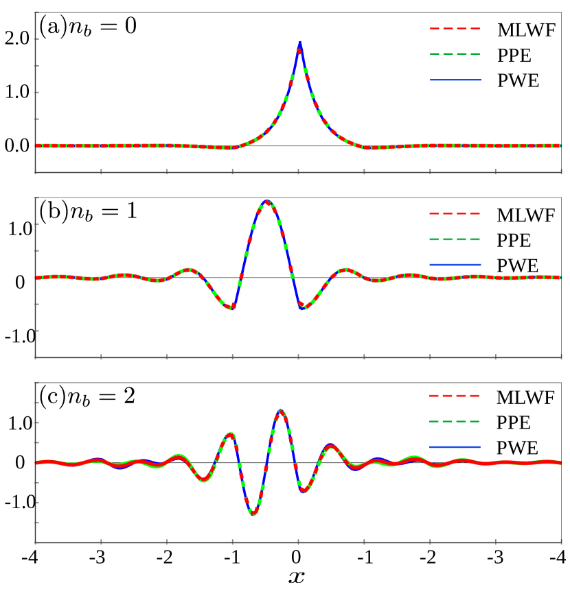
Figure 8: Profiles of MLWF, PPE and PWE. $n_{b}$ at the left upper corner of each panel denotes the band index. In all panels, $N=40$, $L=200$ and $V(x)=\sum V_{0}\delta(x-n)$ with $V_{0}=-0.2(2\pi^{2})$ [54].

Fig. 9 is a graphical representation of Eq. (60) and Eq. (61), and it shows shifting PPEs under the same condition employed in Fig. 8(b). The MLWFs and PPEs are shown in thick and thin lines, respectively, and the color of PPEs ($\xi^{\perp C}_{p}(x)=\langle x|x^{\perp C}_{p}\rangle$) changes from blue to red as the parameter $x_{p}$ varies from 0 to 1.

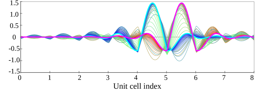
Figure 9: Profiles of MLWF(thick lines colored (red or blue) and shifting PPE (thin lines colored gradually from red to blue), $V(x)=\sum V_{0}\delta(x-n)\ (V_{0}=-0.2(2\pi^{2}))$, $N=40$, $L=200$. The band index $n_{b}=1$.

Table 6 compares the localization indicator $\sigma_{x}^{2}$ calculated with each method. The PPEs and PWEs show as good localization as the known results. When the cost of calculation is taken into account, the methods using PPE and PWE are attractive alternatives.

Table 6: Comparison of spreads, $\sigma_{x}^{2}=\langle W|\{\hat{x}-\langle W|\hat{x}|W\rangle\}^{2}|W\rangle$, obtained from different methods.

Calculation condition			$\sigma_{x}^{2}$
$V_{0}$	Band		Ref. [54]	MLWF	PPE	PWE
$-0.2\times 2\pi^{2}$	0		0.03	0.03	0.03	0.03
$-0.2\times 2\pi^{2}$	1		0.12	0.12	0.12	0.12
$-0.2\times 2\pi^{2}$	2		0.24	0.24	0.24	0.26

VI.2.2 Photonic Systems

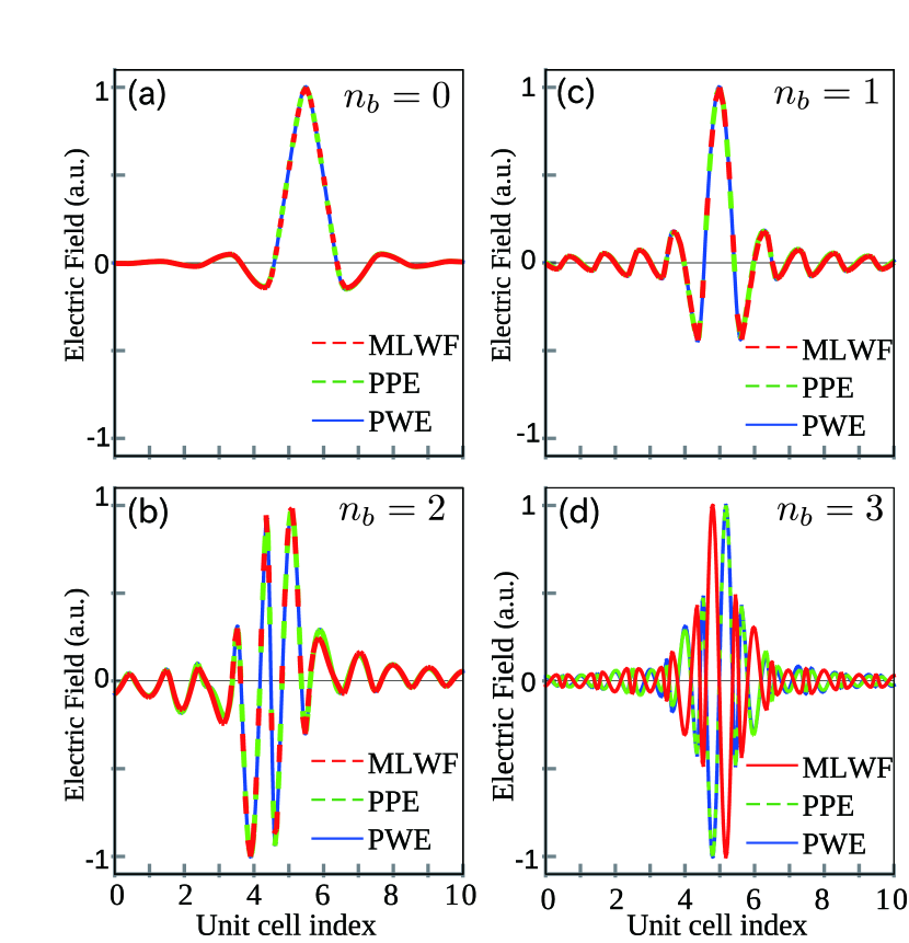
Figure 10: Profiles of MLWF, PPE and PWE. $n_{b}$ at the left upper corner of each panel denotes the band index. In all panels, $N=40$, $L=40$ and $\epsilon(x)=\sum 12\phi_{H}(0.3,x\!-0.35-\!n)$ [51].

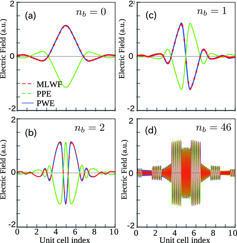
Figure 11: Profiles of electric field for MLWF, PPE and PWE. $n_{b}$ at the left upper corner of each panel denotes the band index. In (a)-(c) $N=40,\ L=40$. In (d) $N=192,\ L=96$. In all panels, $\epsilon(x)=\sum 5\phi_{H}(1/2,x\!-\!na),\ a$: cell length[15].

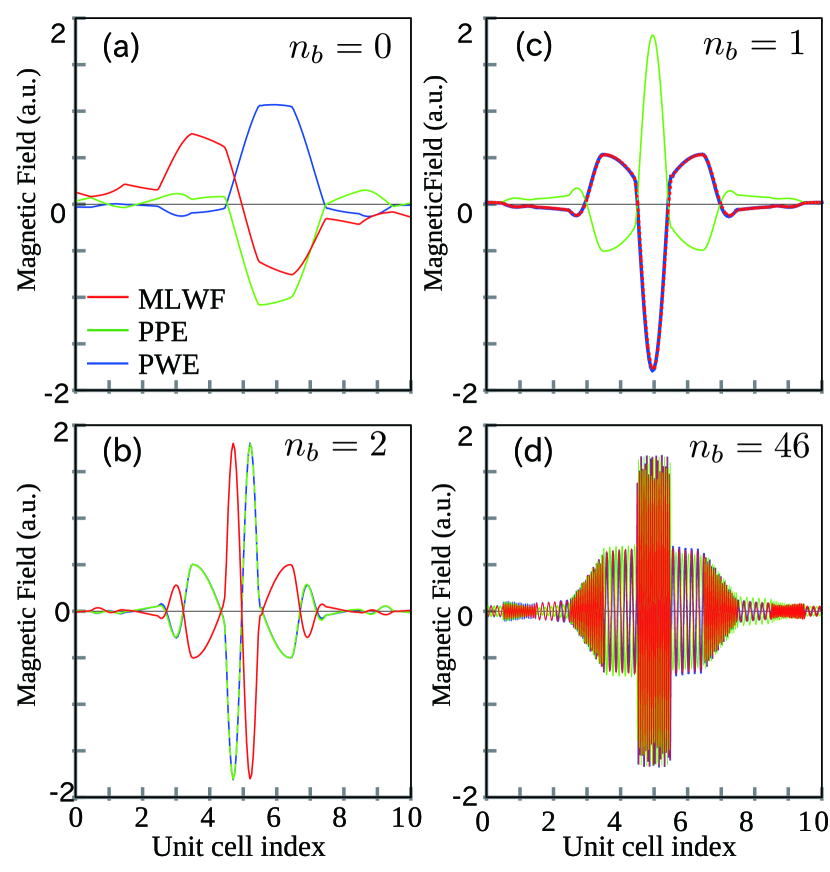
Figure 12: Profiles of magnetic field for MLWF, PPE and PWE. $n_{b}$ at the left upper corner of each panel denotes the band index. In (a)-(c) $N=40,\ L=40$. In (d) $N=192,\ L=96$. In all panels, $\epsilon(x)=\sum 5\phi_{H}(1/2,x\!-\!na),\ a$: cell length[15].

This section focuses on comparing MLWFs, PPEs and PWEs with the preceding results done for photonic crystals. The dielectric susceptibility functions used in Figs. 10 to 12, are listed in Table 5, and all MLWFs, PPEs and PWEs show good agreements, in shape and position, with the preceding results[15, 51]. The disagreement with MLWF shown in Fig. 12(a) will be discussed later in Sec. VI.2.3.

Even in the 46th band of Figs. 11 and 12 with very high wave number, all WFs calculated in this paper show good agreements with the preceding results calculated with $(N,\ L)=(512,\ 99)$. As is noted in Secs. III.3.1, $\sigma^{2}_{x}$ is actually calculated to find out the maximally localized PPE and PWE in Figs. 11(d) and 12(d).

VI.2.3 Note on 0th band MLWF in Fig. 12(a)

The MLWF drawn in red in Fig. 12(a) disagrees with the PPE, PWE and the result shown in Ref. [15]. The WF drawn in red in the present calculation is actually the eigenfunction of the position operator but not the maximally localized WF. As described in Ref. [55], the magnitude of the WFs do not decrease exponentially, thereby inappropriately influenced by the boundary condition through the eigenvalue equation, Eq. (186).

On the other hand, PPEs and PWEs show good agreements with results seen in Refs. [55, 15], since they are calculated locally with little influence from the boundary.

VI.3 WFs in Composite Band Systems

The section focuses on an electronic composite band system and the comparisons of MLWFs, PPEs and PWEs with the results shown in Ref. [56].

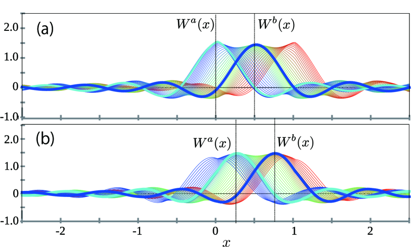
Figure 13: Searching maximally localized position with PPE in two-band systems consisting of $0$th and first energy bands. The superscript $a$ and $b$ on $W(x)$ denote the series. In (a) and (b) $N=40,L=100$ and $V(x)=\sum V_{0}\delta(x-n)$, in (a) with $V_{0}=-0.661$ and in (b) with $V_{0}=+0.661$ [56]. It shows the maximum point of one series coincides with the zero of the other.

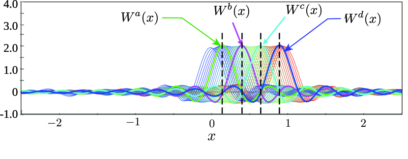
Figure 14: Searching maximally localized position with PPE in four-band system consisting of $0$th to third energy bands. The superscript $a$ to $d$ on $W(x)$ denote the series. In the panel, $N=40,L=100$ and $V(x)=\sum V_{0}\delta(x-n)$, with $V_{0}=0.661$ [56]. It shows the maximum point of one series coincides with the zero of others.

Table 7: Comparison of spreads, $\sigma_{x}^{2}=\langle W|\{\hat{x}-\langle W|\hat{x}|W\rangle\}^{2}|W\rangle$, obtained from different methods.

Calculation condition			$\sigma_{x}^{2}$
$V_{0}$	Bands		Ref. [56]	MLWF	PPE	PWE
0.661	0 to 3		0.29	0.29	0.46	0.46
-0.661	0 to 1		0.27	0.27	0.37	0.37

VI.3.1 Comparison of the Results

By using Eq. (67), Fig. 13(a) shows how shifting PPEs coincide with MLWFs in the same way Fig. 9 are drawn. In addition to the maximally localized WF near the origin of the Fig. 13(a), the second maximally localized WF is observed near $x_{p}=0.5$, which is not seen in Ref. [56]. This existence of two MLWFs in one unit cell is simply a reflection of the completeness of the MLWFs in $\mathcal{H}_{B_{12}}=\mathcal{H}_{B_{1}}+\mathcal{H}_{B_{2}}$; it takes two eigenfunctions per unit cell to span$\mathcal{H}_{B_{12}}$.

By setting $V_{0}=+0.661$, Fig. 13(b) is drawn in the same manner (which does not appear in Ref. [56]). The figure also shows two peaks on the envelope in a unit cell and the MLWFs and PPEs coincide.

By defining four-band PPEs in the same manner, Fig. 14 demonstrates the PPEs almost coincide with four four-band MLWFs, which are also shown in Ref. [56]. Table 7 compares the localization measure obtained by MLWF, PPE, PWE with the preceding results. The PPE and PWE again show decent agreement with the others.

Most importantly, by reflecting Eq. (196) and the accuracy of PPEs as an alternative to MLWF, at the maximum position of an MLWF and PPE, the other MLWFs and PPEs have their zeroes.

VII Summary

VII.1 Position Eigenfunctions

Position scaling-eigenfunctions with practically compact supports and relatively good interpolation capability are generated from compactly supported orthonormal SFs.

The matrix elements of the operators, especially those of the kinetic energy operator, are obtained without performing differentiation. This relaxes the condition on differentiability of the original compact support SFs.

VII.2 MLWF, PPE and PWE

When the MLWFs are composed of all BFs of all energy bands, the MLWFs and the position scaling-eigenfunctions are identical.

In single band cases, the difference between PPEs and MLWFs is the choice of anti-phases to cancel the phases of the BFs. In case the error estimated by Eq. (92) is small enough, it is sufficient to use PPEs as an alternative to MLWFs.

The relationship between the zeros and maxima of MLWFs and the corresponding PPEs are explained in relation to the inter- and intra-series orthogonality of MLWFs.

One of the advantages of using PPE is that it does not take additional localized orbits/bases other than the position scaling-eigenfunctions. Especially, in cases the centers of the MLWFs do not coincide with the centers of the atoms[30] and photonic crystal cases, in which there is no inherently localized orbits[19], the PPEs seem to be particularly useful.

The other advantage followed from the investigation of the PPE and PWE is the variable to be maximized has a simple form:

$$\begin{split}&F(m)=\sum_{k}\left|c_{m,k}\right|^{2}\ \left(m=p\ \mathrm{mod}\ N\right).\\ \end{split}$$ (104)

And hence it is expected to be computationally inexpensive.

VII.3 Numerical Scheme

The results well agree with the preceding results, in some cases, with less calculation cells in a unit cell.

The number of the bases, i.e., the position scaling-eigenfunctions in one unit cell and the spatial resolution are equivalent, and hence all spatial information on the system are readily stored in $\{c^{n}_{k,m}\}$ position-by-position.

The particular advantage of the numerical scheme developed is to diagonalize the potential energy, when it is composed only of the position operator. Because of this, once the discretization of the Hamiltonian is done, no actual integration is needed. In addition, the kinetic energy part is band diagonal with constant matrix elements and hence the eigenvalue and vectors are easy to obtain.

VII.4 Future Direction

On the mathematical side, the mathematical mechanism of giving compactly supported SFs a higher degree of differentiability than the Hölder exponent through Eq. (110) will have to be rigorously investigated. A method to estimate the error of PPEs with respect to the MLWFs in composite band cases has also to be developed to the degree performed in single band cases.

One of the most important steps to take is to extend the entire scheme to 2 and 3D. For the purpose, the multidimensional scaling functions may have to be constructed in the way described in Ref. [57], so that the symmetry of the system is inherent to the basis set. If the proposed scheme is not seriously restricted by the extension, it allows actually to calculate the measurable physical properties of materials, such as electric polarization, chemical bonding known to be closely related to the configuration of MLWFs [2, 3, 4, 5, 2, 6, 7, 8, 9, 5, 2, 10, 9, 6, 8, 7, 11, 12]. Concrete estimates of the efficacy of the method, such as the accuracy, speed and portability, in relation to the existing codes can be performed at this future stage.

Since the obtained position eigenfunctions are also scaling functions and satisfy the two-scale relation, the computational speed of the numerical procedures such as the maximum point searching, solving the eigenvalue problems associated with Schrödinger equations, can be improved by combining the multiscale nature, i.e., iterative methods and mesh refinement, in the future step.

Appendix A Matrix Elements of Operators

A.1 General Strategy

If an operator $\hat{A}$ satisfies the following dilation relation:

$$(x\rightarrow 2x)\longmapsto(\hat{A}\rightarrow 2^{n}\hat{A}).$$ (105)

The two-scale relation becomes linear equations for the matrix elements of the operator:

$$\begin{split}A_{m,n}&=\langle m|\hat{A}|n\rangle\\ &=\int\phi(x-m)A(x,\frac{1}{i}\frac{\partial}{\partial x})\phi(x-n)dx\\ &=2\sum_{l,k}h_{l}h_{k}\int\phi(2x-2m-l)\\ &\quad\quad A(x,\frac{1}{i}\frac{\partial}{\partial x})\phi(2x-2n-k))dx\\ &=2\sum_{l,k}h_{l}h_{k}\int\phi(y-2m-l)\\ &\quad\quad A(2^{-1}y,\frac{1}{i}\frac{\partial}{\partial\left(2^{-1}y\right)})\phi(y-2n-k)d\left(\frac{y}{2}\right)\\ &=2\sum_{l,k}h_{l}h_{k}\int\phi(y-2m-l)\\ &\quad\quad 2^{-n}A(y,\frac{1}{i}\frac{\partial}{\partial y})\phi(y-2n-k)d\left(\frac{y}{2}\right)\\ &=2^{-n}\sum_{l,k}h_{l}h_{k}A_{2m+l,2n+k}.\end{split}$$ (106)

It only takes linear algebraic calculations to obtain the matrix elements, since the final form of the equations involves neither integration nor differentiation.

A.2 Position Operator $\tilde{x}$

A.2.1 Matrix Elements of $\tilde{x}$

Since the following holds:

$$(x\rightarrow 2x)\longmapsto(\hat{x}^{n}\rightarrow 2^{n}\hat{x}^{n}),$$ (107)

Eq. (13) is a special case of Eq. (106). The solution, $X_{r}=\langle r|\hat{x}|0\rangle$, is listed on Table 8. From the table, $X_{m,n}$ is calculated as follows:

$$X_{m,n}=m+X_{r}\quad(r=m-n).$$ (108)

Table 8: Matrix elements of position operator $X_{r}=\langle r|\hat{x}|0\rangle$ obtained with different SFs.

		$X_{0}$	$X_{1}$	$X_{2}$	$X_{3}$	$X_{4}$
1. SF
a. Sy4		4.126	-0.023	-0.033	0.000	0.000
b. Db2		0.771	-0.071	-0.002	0.000	0.000
c. Db3		1.022	-0.121	0.019	-0.001	0.000
d. Db4		1.266	-0.164	0.039	-0.005	0.000

A.2.2 Matrix Elements of $\tilde{x}^{2}$

Table 9 shows the matrix elements:

$$\sigma^{2}_{r}=\langle r|\hat{x}^{2}|0\rangle.$$

They are revisited in Appendix 115 to discuss the interpolation capability of the position scaling-eigenfunctions.

Table 9: Matrix elements of $\hat{x}^{2}$, $\sigma^{2}_{r}=\langle r|\hat{x}^{2}|0\rangle$, obtained with different SFs.

		$\sigma^{2}_{0}$	$\sigma^{2}_{1}$	$\sigma^{2}_{2}$	$\sigma^{2}_{3}$	$\sigma^{2}_{4}$
1. SF
a. Sy4		0.103	-0.285	-0.314	0.004	0.000
b. Db2		0.077	-0.206	-0.003	0.000	0.000
c. Db3		0.094	-0.414	0.087	-0.001	0.000
d. Db4		0.119	-0.647	0.207	-0.031	0.000

A.3 Momentum Operator $\tilde{p}$

A.3.1 Computation

Since:

$$(x\rightarrow 2x)\longmapsto(\hat{p}^{n}\rightarrow 2^{-n}\hat{p}^{n}),$$ (109)

the following equations for the matrix elements of $\hat{p}^{n}$ are obtained from Eq. (106):

$$\begin{split}P_{m,n}&=\frac{1}{2}\langle m|\hat{p}^{n}|n\rangle\\ &=2^{n}\sum_{l,k}h_{l}h_{k}P_{2m+l,2n+k}.\end{split}$$ (110)

As in the case of the position operator, $\{P_{r}\}$ is defined:

$$P_{r}=P_{m+r,m}.$$ (111)

By substituting the above to Eq. (110), we have the equation for $\{P_{r}\}$:

$$P_{r}=2^{n}\sum_{k,q}h_{k}h_{k+2r-q}P_{q}.$$ (112)

Unlike $\hat{x}$, $\hat{p}$ is translationally invariant, thus the equation becomes homogeneous eigenvalue equation:

$$\begin{array}[]{l}\mathbf{K}\cdot\bm{P}=\rho\bm{P},\\ \left[\mathbf{K}\right]_{r,q}=\sum_{k}h_{k}h_{k+2r-q},\\ \left[\bm{P}\right]_{r}=P_{r},\end{array}$$ (113)

and hence the physical substance of $\{P_{r}\}$ depends on $\rho$:

$$P_{r}=\langle r|\hat{p}^{n}|0\rangle,\quad n=-\log_{2}\rho.$$

If $\rho=2$, it is the matrix elements of the momentum operator, if $\rho=4$, it is those of the kinetic energy operator. Since Eq. (112) is homogeneous, supplemental conditions have to be provided to determine their magnitude:

$$\begin{split}\sum_{r}rP_{r}=\frac{1}{i}&\quad(\mathrm{for\ }\rho=2),\\ \sum_{r}r^{2}P_{r}=-2&\quad(\mathrm{for\ }\rho=4).\end{split}$$ (114)

Thus, the series $\{P_{r}\}$ is uniquely determined.

A.3.2 Results and Implication

Table 10: Matrix elements of $i\hat{p}$, $iP_{r}=\langle r|\ i\hat{p}|0\rangle$ obtained with different SFs (eigenvalue $\rho=2$).

		$iP_{0}$	$iP_{1}$	$iP_{2}$	$iP_{3}$	$iP_{4}$
1. SF
a. Sy4		0.000	-0.793	0.192	-0.034	0.002
b. Db2		0.000	-0.667	0.083	0.00	0.00
c. Db3		0.000	-0.745	0.145	-0.015	0.000
d. Db4		0.000	-0.793	0.192	-0.034	0.002

Table 11: Matrix elements of $\hat{p}^{2}/2$, $P_{r}=\langle r|\ \hat{p}^{2}/2|0\rangle$ obtained with different SFs (eigenvalue $\rho=4$).

		$-P_{0}$	$-P_{1}$	$-P_{2}$	$-P_{3}$	$-P_{4}$
1. SF
a. Sy4		-4.166	2.642	-0.698	0.151	-0.011
b. Db2		-6/0	4/0	-1/0	0/0	0/0
c. Db3		-5.268	3.390	-0.876	0.114	0.005
d. Db4		-4.166	2.642	-0.698	0.151	-0.011

The numerically obtained series $\{P_{r}\}$ corresponding to the momentum and the kinetic energy operators are listed in the Table 10 and Table 11, respectively.

The following conventional calculation to obtain $\{P_{r}\}$ requires the Hölder exponent of the SFs to be greater than $n$:

$$\begin{split}P_{r}&=\langle r|\int dy|y\rangle\langle y|\hat{p}^{n}\int dx|x\rangle\langle x|n=0\rangle\\ &=\int dy\int dx\langle r|y\rangle\langle y|x\rangle\left(\frac{1}{i}\right)^{n}\frac{{\partial}^{n}}{\partial x^{n}}\langle x|n=0\rangle\\ &=\left(\frac{1}{i}\right)^{n}\int dx\phi(x-r)\frac{\partial\phi(x)}{\partial x}.\end{split}$$ (115)

On the other hand, the current method does not have explicit conditions on a differentiability per se, since no actual differentiation takes place in Eq. (106). In fact, it works well with the SFs having lower Hölder exponents such as Daubechies-3, as shown in Table 2.

The reason seems to be Eq. (115) forces to calculate the unwanted higher resolution components out of $\mathcal{H_{S}}$, which are discarded when coming back to $\mathcal{H_{S}}$. In Eq. (106), contrary, the higher resolution parts are dealt with by the two-scale relation and algebra, but not by differentiation.

In the case of Db2 ($\mathrm{C}^{0.5}$-continuous), however, the eigenvector corresponding to the kinetic energy is:

$$\bm{P}=[1,-4,6,-4,1]^{\mathrm{T}},$$ (116)

and this fails to satisfy the condition given by Eq. (114).

The differentiability in the sense of Eq. (112) will have to be investigated further.

A.3.3 Commutation Relation

Since the operators $\tilde{x}$ and $\tilde{p}$ are defined in a space spanned by a finite number of basis vectors:

$$\mathrm{Tr}\{\tilde{x}\tilde{p}\}=\mathrm{Tr}\{\tilde{p}\tilde{x}\},$$ (117)

and hence, they cannot satisfy the usual commutation relations such as:

$$[\tilde{p},\tilde{x}]=-i.$$ (118)

In stead, they satisfy the following commutation relation:

$$\begin{split}\sum_{l}&P_{m,l}X_{l,n}-X_{m,l}P_{l,n}\\ =&\sum_{l}P_{m-l}(X_{l-n}+n\delta_{l,n})-(X_{m-l}+m\delta_{m,l})P_{l-n}\\ =&(m-n)P_{m-n}.\end{split}$$ (119)

Appendix B Eigenvectors of the Operators

B.1 Position Eigenvalue

B.1.1 From translational symmetry

A position eigenvector satisfies the following:

$$\tilde{x}|x_{n}\rangle=x_{n}|x_{n}\rangle.$$ (120)

By introducing the translation operator:

$$T(\beta)=e^{i\beta\hat{p}}\ (\beta\in\mathbb{R}),$$ (121)

it is obvious:

$$\hat{T}(1)\tilde{x}|x_{n}\rangle=\hat{T}(1)\{x_{n}|x_{n}\rangle\}=x_{n}\{\hat{T}(1)|x_{n}\rangle\}.$$ (122)

On the other hand, if $\hat{T}(1)$ is applied first to $\tilde{x}$:

$$\begin{split}\hat{T}(1)\tilde{x}|x_{n}\rangle&=\hat{T}(1)\tilde{x}\hat{T}^{\dagger}(1)\hat{T}(1)|x_{n}\rangle\\ &=(\tilde{x}+1)\{\hat{T}(1)|x_{n}\rangle\}.\end{split}$$ (123)

By comparing the two equations, we get:

$$\begin{split}x_{n}\{\hat{T}(1)|x_{n}\rangle\}&=(\tilde{x}+1)\{\hat{T}(1)|x_{n}\rangle\}\\ \tilde{x}\{\hat{T}(1)|x_{n}\rangle\}&=(x_{n}-1)\{\hat{T}(1)|x_{n}\rangle\}.\\ \end{split}$$ (124)

And hence

$$\begin{array}[]{c}\hat{T}(1)|x_{n}\rangle=|x_{n-1}\rangle,\\ x_{n}=x_{n-1}+1.\end{array}$$ (125)

From the above, $x_{n}$ has to have the following form with an unknown $C_{0}$:

$$x_{n}=C_{0}+n.$$ (126)

B.1.2 With trace of the operator

On the other hand by using Eq. (15), we have:

$$\begin{split}\sum_{n}x_{n}&=Tr(\tilde{x})\\ &=\sum_{n=-N}^{N}X_{n,n}\\ &=(2N+1)X_{0}.\end{split}$$ (127)

By comparing the above and Eq. (126)

$$\begin{array}[]{c}C_{0}=X_{0},\\ x_{n}=n+X_{0}.\end{array}$$ (128)

B.2 Position Eigenvector

B.2.1 Equation

The position eigenvectors are expressed by a unitary transformation and the SFs:

$$|x_{n}\rangle=\sum_{n}\xi_{n,m}|m\rangle.$$ (129)

By translating an eigenvector by 1:

$$\begin{split}|x_{n-1}\rangle&=\hat{T}(1)|x_{n}\rangle\\ &=\sum_{m}\xi_{n,m}\hat{T}(1)|m\rangle\\ &=\sum_{m}\xi_{n,m}|m-1\rangle\\ &=\sum_{m}\xi_{n,m+1}|m\rangle.\end{split}$$ (130)

On the other hand, by definition:

$$|x_{n-1}\rangle=\sum_{m}\xi_{n-1,m}|m\rangle.$$ (131)

From this, we find:

$$\xi_{n-1,m}=\xi_{n,m+1},$$

and the matrix $\{\xi_{n,m}\}$ is simplified to a series:

$$\xi_{n,m}\rightarrow\xi_{n-m}.$$

By combining the above with Eq. (12) and Eq. (128) the equation for $\{\xi_{n}\}$ becomes:

$$\sum_{n}\{X_{m-n}\xi_{n-p}+m\delta_{m,n}\xi_{n-p}\}=x_{p}\xi_{m-p}.$$ (132)

Since the solution has the translational symmetry, it is enough to solve for $p=0$. From Eq. (126) regarding the eigenvalue and Eq. (128) regarding the diagonal elements, Eq. (132) has $X_{0}$ on the both side of it. By subtracting $X_{0}$ from the both side of Eq. (132), or equivalently setting $X_{0}=0$ and $x_{p=0}=0$, we get:

$$\sum_{n}\{X_{m-n}\xi_{n}+m\delta_{m,n}\xi_{n}\}=0.\\$$ (133)

B.2.2 Analytical Solution Procedure

Although Eq. (133) for $\{\xi_{n}\}$ is numerically solvable with a math library such as GSL[43], the analytical solution gives more insight into the position eigenvectors.

Since Eq. (133) has a form of convolution, Fourier transformation makes it easier to solve:

$$\sum_{m,n}X_{m-n}e^{-im\omega}e^{in\omega}\xi_{n}e^{-in\omega}+\sum_{m,n}m\delta_{m,n}\xi_{n}e^{-im\omega} =0.$$ (134)

By defining the following two functions:

$$X(\omega)=\sum_{m}X_{m}e^{-im\omega},$$ (135)

$$\xi(\omega)=\sum_{m}\xi_{m}e^{-im\omega},$$

we get:

$$X(\omega)\xi(\omega)+i\frac{{\partial}}{\partial\omega}\xi(\omega) =0.$$ (136)

With $C$ as the normalization factor, the solution is thus:

$$\begin{split}\xi(\omega)&=C\exp\left(i\sum_{m}\int^{\omega}d\Omega X_{m}e^{im\Omega}\right)\\ &=C\exp\left(-\sum_{m\neq 0}\frac{X_{m}}{m}e^{im\omega}\right).\end{split}$$ (137)

By using the Bessel function of the first kind $J_{n}(z)$, the following holds[58]:

$$\begin{split}e^{-(\frac{X_{m}}{m}e^{im\omega}-\frac{X_{m}}{m}e^{-im\omega})}&=e^{-2iX_{m}\sin(m\omega)}\\ &=\sum_{n=-\infty}^{+\infty}J_{n}\left(-\frac{2X_{m}}{m}\right)e^{inm\theta}.\\ \end{split}$$ (138)

By defining:

$$Y_{m}=-\frac{X_{m}}{m},$$ (139)

$\xi(\omega)$ is thus factorized as follows:

$$\begin{split}\xi(\omega)=C&\left\{\sum_{n_{1}=-\infty}^{+\infty}J_{n_{1}}(Y_{1})e^{in_{1}\omega}\right\}\left\{\sum_{n_{2}=-\infty}^{+\infty}J_{n_{2}}(Y_{2})e^{i2n_{2}\omega}\right\}\\ &...\left\{\sum_{n_{T}=-\infty}^{+\infty}J_{n_{M}}(Y_{M})e^{iMn_{M}\omega}\right\}.\\ \end{split}$$ (140)

By segregating the terms in Eq. (140) exponent-by-exponent, we have:

$$\begin{split}\xi_{n}&=\frac{1}{2\pi}\int_{0}^{2\pi}\xi(\omega)e^{in\omega}d\omega\\ &=C\sum_{n_{1}+2n_{2}+...+Mn_{M}=-n}J_{n_{1}}(Y_{1})J_{n_{2}}(Y_{2})...J_{n_{M}}(Y_{M}).\end{split}$$ (141)

The following is an example hand calculation of Pdb2:

$$\begin{split}\xi(\omega)\simeq&(J_{2}(Y_{1})e^{-2i\omega}-J_{1}(Y_{1})e^{-i\omega}\\ &\quad+J_{0}(Y_{1})+J_{1}(Y_{1})e^{i\omega}+J_{2}(Y_{2})e^{2i\omega})\\ &(J_{2}(Y_{2})e^{-4i\omega}-J_{1}(Y_{2})e^{-2i\omega}\\ &\quad+J_{0}(Y_{2})+J_{1}(Y_{2})e^{2\omega}+J_{2}(Y_{2})e^{4i\omega})\\ \simeq&(0.0025e^{-2i\omega}-0.0708e^{-i\omega}\\ &\quad+0.9950+0.0708e^{i\omega}+0.0025e^{2i\omega})\\ &\left(-0.0001e^{-2i\omega}+1.0000+0.0001e^{2\omega}\right)\\ \simeq&0.0015e^{-2i\omega}-0.0709e^{-i\omega}\\ &+0.9950+0.0708e^{i\omega}+0.0035e^{2i\omega},\end{split}$$ (142)

where the values of $\{Y_{m}\}$ are obtained from Table 8 through Eq. (139). After paying attention to Eq. (135), we have $\{\xi_{n}\}$ approximately equals to the corresponding series shown in Table 1.

B.2.3 Rate of Decay of $\xi_{n}$

If

$$F^{m}(\omega)=\left\{\sum_{n=-\infty}^{+\infty}J_{n}(Y_{m})e^{inm\omega}\right\}.$$ (143)

is analytic, $\xi(\omega)$ is also analytic[59] and hence $\xi_{n}$ decays faster than any polynomial[60].

The decay of the following Fourier series is, therefore, first estimated to show $F^{m}(\omega)$ is analytic:

$$f^{m}_{nm}=\frac{1}{2\pi}\int F^{m}(\omega)e^{-inm\omega}d\omega.$$ (144)

When $|n|$ is large enough to meet:

$$0<|Y_{m}|\ll\sqrt{n+1},\\$$ (145)

the following holds[61]:

$$J_{n}(Y_{m})\sim\operatorname{sign}(n)^{|n|}\frac{1}{|n|!}\left(\frac{Y_{m}}{2}\right)^{|n|}.$$ (146)

And hence

$$\begin{split}|f^{m}_{nm}|&=\frac{1}{|n|!}\left|\frac{Y_{m}}{2}\right|^{|n|}\\ &=\frac{1}{\sqrt{2\pi|n|}}\left(\frac{e}{|n|}\right)^{|n|}\left|\frac{Y_{m}}{2}\right|^{|n|}\\ &=\frac{1}{\sqrt{2\pi|n|}}\left(\frac{e\left|Y_{m}\right|}{2|n|}\right)^{|n|}.\end{split}$$ (147)

From Table 8

$$\left(\frac{e\left|Y_{m}\right|}{2|n|}\right)^{|n|}<1,$$ (148)

and hence positive constants $A$ and $c_{0}$ satisfying the following system of inequality exist:

$$|f^{m}_{nm}|<Ae^{-c_{0}|n|}\ \quad(n\in\mathbb{Z}).$$ (149)

By defining $r=nm$, $c_{1}=c_{0}/m$, we have

$$|f^{m}_{r}|<Ae^{-c_{1}|r|}\ \quad(r\in\mathbb{Z}).$$ (150)

Thus, $F^{m}(\omega)$ is analytic[60], and hence $\xi(\omega)$ is analytic and $\xi_{n}$ decays faster than any polynomial of $r$ as $r$ goes to infinity.

B.2.4 Normalization of $\xi_{m}$ and Convergence of the Sum

The normalization coefficient $C$ is determined as follows:

$$\begin{split}\delta_{mn}=&\langle m|\hat{1}|n\rangle\\ =&\langle m|\{\sum_{p=-\infty}^{\infty}|x_{p}\rangle\langle x_{p}|\}|n\rangle\\ =&\sum_{p}\xi_{m-p}\xi_{n-p}\\ =&\frac{C^{2}}{(2\pi)^{2}}\!\!\!\sum_{p=-\infty}^{\infty}\!\!\!\int e^{i(m-p)\omega_{1}}\xi(\omega_{1})d\omega_{1}\int e^{i(n-p)\omega_{2}}\xi(\omega_{2})d\omega_{2}\\ =&\frac{C^{2}}{(2\pi)^{2}}\!\!\!\int\!\!d\omega_{1}\!\!\!\int\!\!\!d\omega_{2}\!\!\!\sum_{p=-\infty}^{\infty}\!\!\!e^{-ip(\omega_{1}+\omega_{2})}\xi(\omega_{1})\xi(\omega_{2})e^{in\omega_{2}}e^{im\omega_{1}}\\ =&\frac{C^{2}}{2\pi}\int d\omega_{1}\xi(\omega_{1})\xi(-\omega_{1})e^{i(m-n)\omega_{1}}\\ =&\frac{C^{2}}{2\pi}\int d\omega_{1}e^{i(m-n)\omega_{1}}\\ =&C^{2}\delta_{m,n}.\\ \end{split}$$ (151)

Thus,

$$|C|=1.$$ (152)

B.2.5 Convergence of $\sum\xi_{m}$

Since $X_{m}/m$ is antisymmetric with respect to $m$, summing Eq. (141) from $-\infty$ to $\infty$ gives:

$$\begin{split}\sum_{m=-\infty}^{\infty}\xi_{m}&=\frac{1}{2\pi}\int 2\pi\delta(\omega)\xi(\omega)d\omega\\ &=\xi(0)=\exp\left(-\sum_{m\neq 0}\frac{X_{m}}{m}\right)=1.\end{split}$$ (153)

B.3 Position Eigenvector as Scaling Function

By applying the two-scale relation to the position eigenfunctions:

$$\begin{split}\xi(x)&=\sum_{p}\xi_{p}\phi(x-p)\\ &=\sqrt{2}\sum_{p}\xi_{p}\sum_{n}h_{n}\phi(2x-2p-n),\end{split}$$ (154)

and utilizing the following:

$$\begin{split}\phi(x)&=\langle x|0\rangle\\ &=\langle x|\sum_{p}|x_{p}\rangle\langle x_{p}|0\rangle\\ &=\sum_{p}\xi_{p}(x)\xi_{-p},\\ \end{split}$$ (155)

we have:

$$\begin{split}\sqrt{2}\sum_{p}\xi_{p}&\sum_{n}h_{n}\phi(2x-2p-n)\\ &=\sqrt{2}\sum_{p}\xi_{p}\sum_{n}h_{n}\sum_{q}\xi_{-q}\xi(2x-2p-n-q)\\ &=\sqrt{2}\sum_{p,n,q}\xi_{p}h_{n}\xi_{q}\xi(2x-2p-n+q)\\ &=\sqrt{2}\sum_{p,n,q}\xi_{p}h_{l-2p+q}\xi_{q}\xi(2x-l).\end{split}$$ (156)

Thus, we have:

$$\begin{split}&\xi(x)=\sqrt{2}\sum_{l}\eta_{l}\xi(2x-l),\\ \end{split}$$ (157)

where

$$\begin{split}\quad\eta_{l}=\sum_{p,q,l}\xi_{p}\xi_{q}h_{q+l-2p}.\end{split}$$ (158)

Therefore, the position eigenfunctions turn out to be scaling functions. The central part of $\{\eta_{l}\}$ is listed in Table 12 and the wavelets corresponding to the position scaling-eigenfunctions are shown in Fig. 15.

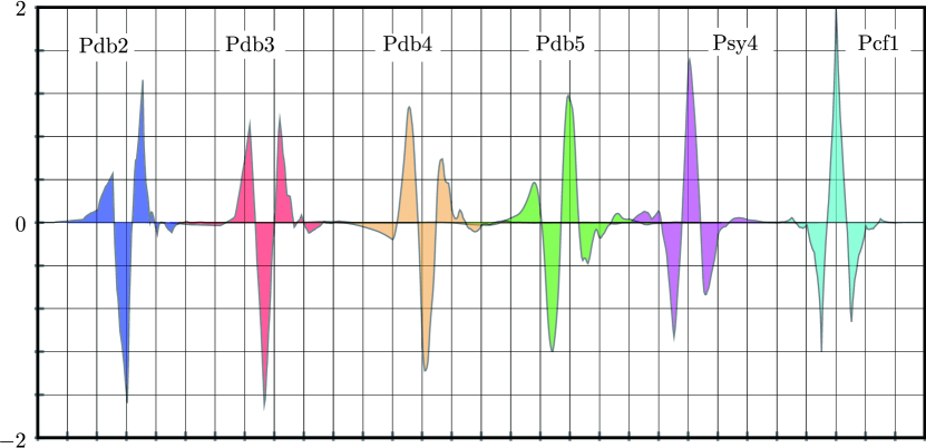
Figure 15: Position wavelets. From left to right, wavelet of Pdb2, Pdb3, Pdb4, Pdb5, Psy4 and Pcf1.

Table 12: Central part of $\{\eta_{r}\}$ corresponding to the position eigenfunction indicated in the first column.

	$\eta_{-3}$	$\eta_{-2}$	$\eta_{-1}$	$\eta_{0}$	$\eta_{1}$	$\eta_{2}$	$\eta_{3}$
1. SF
a. Psy4	-0.026	-0.096	0.316	0.808	0.480	-0.039	-0.066
b. Pdb2	-0.037	-0.023	0.526	0.822	0.193	-0.083	0.022
c. Pdb3	-0.046	-0.062	0.376	0.827	0.400	-0.089	-0.015
d. Pdb4	-0.038	-0.093	0.244	0.772	0.572	-0.018	-0.074

In comparison with the original compact support SFs, the position scaling-eigenfunctions have the following properties: (1) Infinite support length. The position scaling-eigenfunctions in real space decay exponentially, but the support is no longer compact. (2) Substantially small $\sigma_{0}^{2}$. Despite the infinitely wide supports of the position scaling-eigenfunctions, $\sigma_{0}^{2}$s are nearly identical to those of the original compactly supported SFs (see Tables 9 and 13). (3) Substantially small $\sigma_{r}^{2}(r\neq 0)$. From the tables, the position scaling-eigenfunctions are closer to the eigenvector of $\hat{x}^{2}$ than the original compactly supported SFs are, since the off-diagonal parts are in general substantially smaller.

Table 13: Matrix elements of $\hat{x}^{2}$, $\sigma^{2}_{r}=\langle x_{r}|\hat{x}^{2}|x_{0}\rangle$, obtained with different position scaling-eigenfunctions.

		$\sigma^{2}_{0}$	$\sigma^{2}_{1}$	$\sigma^{2}_{2}$	$\sigma^{2}_{3}$	$\sigma^{2}_{4}$
1. SF
a. Psy4		0.108	-0.077	0.026	0.000	0.000
b. Pdb2		0.088	-0.040	-0.002	0.001	0.000
c. Pdb3		0.102	-0.064	0.009	0.004	-0.001
d. Pdb4		0.116	-0.082	0.024	0.002	-0.003

B.4 Transformation of Position Scaling-Eigenvector in Physical and Numerical Coordinate Systems

The formulation can be done either in the physical or in numerical domain. In the numerical domain, the unit cell length coincides with the number of division in one unit cell $N$. It disagrees with the convention, but the formulation becomes simplest. When the physical domain is chosen to keep the unit cell length at $1$, the following constant for conformation $c$ has to be chosen,

$$\langle x|x_{p}\rangle=c\xi(N(x-x_{p})).$$ (159)

A choice of $c$ makes some relationships simple and others a little more complex. In the paper, $c$ is chosen so that the basis set becomes orthonormal. The resulting relationships between variables and functions are listed in Table 14 for convenience.

Table 14: Correspondence of parameters, variables, functions, inner products and operator between physical and numerical domains.

	Domain
	Physical	Numerical
Unit cell length	$1$	$N$
Range	$0\leq x<L$	$0\leq x<NL$
$\Delta x$	$1/N$	$1$
$x_{p}$	$p\Delta x$	$p$
$\langle x|x_{p}\rangle$	$\sqrt{N}\xi(N(x-x_{p}))$	$\xi(x-x_{p})$
$\langle f|x_{p}\rangle$	$f_{p}$	$f_{p}$
$f(x)$	$\sqrt{N}\sum_{p}f_{p}\xi(N(x-x_{p}))$	$\sum_{p}f_{p}\xi(x-x_{p})$
$f(x_{p})$	$\sqrt{N}\{f_{p}+O(\sigma^{2}_{0}/N^{2})\}$	$f_{p}+O(\sigma^{2}_{0})$
$\int dxf(x)g(x)\simeq$	$\sum_{p}f(x_{p})g(x_{p})\Delta x$
$\hat{1}$	$\sum_{p}|x_{p}\rangle\langle x_{p}|$	$\sum_{p}|x_{p}\rangle\langle x_{p}|$
$\langle x_{p}|x_{q}\rangle$	$\delta_{p,q}$	$\delta_{p,q}$
$\int dx\langle x|x_{p}\rangle$	$1/\sqrt{N}$	$1$

B.5 Approximation of Functions and Matrix Elements Using Position eigenvectors’ Properties

A function or signal can be projected onto $\mathcal{H_{S}}$ spanned by a set of SFs $\{|\phi_{p}\rangle\}$:

$$\begin{split}\tilde{f}(x)&=\sum f_{p}\phi(x-p),\\ f_{p}&=\langle\phi_{p}|f\rangle.\end{split}$$ (160)

Certain SFs called interpolation SFs, such as the Shannon SF[62], satisfy:

$$f_{p}=f(p).$$ (161)

This implies the values of an incoming signal or a function on the ticks are by themselves expansion coefficients, thereby substantially reducing the cost of decomposition (albeit, the Shannon SF is hard to employ in practical cases for the slow decay). This section therefore focuses on the interpolation capability of the position scaling-eigenfunctions and the eventual reduction in the potential energy matrix elements.

B.5.1 Interpolation Capability of Position Scaling-Eigenfunctions

In general case, by using a set of general orthonormal scaling functions $\{\phi_{p}(x)\}$, $f_{p}$ is expressed as follows:

$$\begin{split}f_{p}&=\int dxf(x)\phi_{p}(x)\\ &=\int dx\langle x|f(\hat{x})|\phi_{p}\rangle.\end{split}$$ (162)

If $f(x)$ is piece-wise quadratic polynomial over a few calculation cells:

$$f(\hat{x})=a_{0}+a_{1}\hat{x}+a_{2}\hat{x}^{2}.$$ (163)

And if the sampling rate or the resolution is high enough to reconstruct the signal or the function, the operation can be done in $\mathcal{H_{S}}$. Thus, following approximation is valid in the vicinity where Eq. (163) holds:

$$\begin{split}f(\hat{x})|\phi_{p}\rangle&=a_{0}|\phi_{p}\rangle+a_{1}\hat{x}|\phi_{p}\rangle+a_{2}\hat{x}^{2}|\phi_{p}\rangle\\ &=a_{0}|\phi_{p}\rangle+a_{1}(\sum_{r}X_{r}|\phi_{p+r}\rangle+p|\phi_{p}\rangle)\\ &\ +\!\!a_{2}(\sum_{r}\sigma_{r}^{2}|\phi_{p+r}\rangle\!+\!2p\sum_{r}X_{r}|\phi_{p+r}\rangle\!+\!p^{2}|\phi_{p}\rangle)\\ &=\{f(p)+(a_{1}X_{0}+2a_{2}pX_{0}+a_{2}\sigma^{2}_{0})\}|\phi_{p}\rangle\\ &\ +\sum_{r\neq 0}\{(a_{1}+2a_{2}p)X_{r}+a_{2}\sigma_{r}^{2}\}|\phi_{p+r}\rangle\\ &=f_{p}|\phi_{p}\rangle+\sum_{r\neq 0}f_{p}^{r}|\phi_{p+r}\rangle,\end{split}$$ (164)

where

$$\begin{array}[]{l}f_{p}=f(p)+(a_{1}X_{0}+2a_{2}pX_{0}+a_{2}\sigma^{2}_{0}),\\ f_{p}^{r}=(a_{1}+2a_{2}p)X_{r}+a_{2}\sigma_{r}^{2},\end{array}$$ (165)

and the contribution from the higher resolution wavelets are ignored when the operator acts on the kets.

By choosing one of the position scaling-eigenvectors as $\phi(x)$, all elements of $\{X_{r}\}$ become zero. Furthermore, $\sigma_{r}^{2}(r\neq 0)$ shown in Table 13 becomes substantially smaller than those of the original SFs listed in Table 9. And hence:

$$\begin{array}[]{l}f_{p}=f(p)+O(\sigma^{2}_{0}),\\ f_{p}^{r}=0+O(\sigma^{2}_{r}).\end{array}$$ (166)

In the physical domain:

$$\begin{array}[]{l}f_{p}=N^{-1/2}f(x_{p})+O(\sigma^{2}_{0}/N^{2}),\\ f_{p}^{r}=0+O(\sigma^{2}_{r}/N^{2}),\\ x_{p}=p/N\ (L_{0},V_{0}\in\mathbb{R}).\end{array}$$ (167)

B.5.2 Application to BFs

From Eqs. (37) and (166),

$$\begin{split}e^{ikl}e^{ikm\Delta x}c_{m,k}^{n}&=\psi_{k,p}^{n}\\ &\simeq N^{-1/2}\psi_{k}^{n}(x_{p}).\\ \end{split}$$ (168)

And hence,

$$\begin{split}|\psi^{n}_{k}\rangle=N^{-1/2}\sum_{n,k}\psi^{n}_{k}(x_{p})|x_{p}\rangle+O(\sigma^{2}_{0}/N^{2}).\\ \end{split}$$ (169)

It also applies to Wannier functions and in the same way:

$$|W_{l}^{s}\rangle=N^{-1/2}\sum_{p}W_{l}^{s}(x_{p})|x_{p}\rangle+O(\sigma^{2}_{0}/N^{2}).$$ (170)

B.5.3 Application to Potential Energy Matrix Elements

If the potential energy as a function of $x$ is piece-wise quadratic polynomial over a few calculation cells, the matrix elements of operator $V(\hat{x})$ is calculated by utilizing Eq. (164):

$$\begin{split}\langle x_{p_{1}}|V(\hat{x})|x_{p_{2}}\rangle&=\langle x_{p_{1}}|\{V(\hat{x})|x_{p_{2}}\rangle\}\\ &=\langle x_{p_{1}}|\{V(x_{p_{2}})|x_{p_{2}}\rangle\}+O(\sigma^{2}_{0}/N^{2})\\ &=V(x_{p_{2}})\delta_{p_{1},{p_{2}}}+O(\sigma^{2}_{0}/N^{2}).\end{split}$$ (171)

The approximation above is, in effect, equivalent of:

$$V(\hat{x})\rightarrow V(\tilde{x}).$$ (172)

B.5.4 $\delta$-function Potential

When $V(x)$ is given as a $\delta$-function such as:

$$\begin{split}V(x,a)&=V_{0}\delta(x-a),\\ \end{split}$$ (173)

preserving the character of the $\delta$-function as an impulse, rather than the direct projection of the delta function onto the composite band space, is prioritized.

The formal potential operator is calculated as follows:

$$\begin{split}\hat{V}(a)&=\int\!\!\!dx|x\rangle V_{0}\delta(x\!\!-\!\!a)\langle x|\\ &=V_{0}|a\rangle\langle a|,\end{split}$$ (174)

and hence,

$$\begin{array}[]{r}\langle f|\hat{V}(a)|g\rangle=V_{0}f(a)g(a)\quad\left(\forall|f\rangle,|g\rangle\in\mathcal{H}\right).\end{array}$$ (175)

In $\mathcal{H}_{X}$, on the other hand,

$$\begin{array}[]{r}\begin{aligned} \langle f|x_{p}\rangle\langle x_{p}|g\rangle&=f_{p}g_{p}\\ &=\frac{1}{N}f(x_{p})f(x_{p})\quad\left(\forall|f\rangle,|g\rangle\in\mathcal{H}_{X}\right).\end{aligned}\end{array}$$ (176)

Thus, the potential energy operator is discretized to be:

$$\begin{array}[]{c}V_{0}|a\rangle\langle a|\rightarrow NV_{0}|x_{p}\rangle\langle x_{p}|,\\ x_{p}=a,\\ p=a/\Delta x.\end{array}$$ (177)

Eventually, the numerical expression of the $\delta$-function potential becomes as follows:

$$\begin{split}\langle x_{p}|\hat{V}(a)|x_{p_{1}}\rangle=V_{0}N\delta_{p,p_{1}}.\end{split}$$ (178)

Note that if the direct projection of $\hat{V}(a)$ on to $\mathcal{H}_{X}$ is carried out, it will result in a possibly broader potential energy operator as described in Sec. III.4:

$$\begin{split}\sum_{p,q}|x_{p}\rangle\langle x_{p}|\hat{V}(a)|x_{q}\rangle\langle x_{q}|=\sum_{p,q}|x_{p}\rangle\xi_{p}(a)\xi_{q}(a)\langle x_{q}|.\end{split}$$ (179)

B.6 Momentum Eigenvector

In a similar way described in Sec. B.2.2, the momentum eigenvectors are obtained:

$$\begin{array}[]{c}\tilde{P}|k\rangle=P(k)|k\rangle,\\ |k\rangle=\frac{1}{\sqrt{N}}\sum_{n}e^{ikn}|n\rangle,\\ P(k)=\sum_{r}P_{r}e^{ikr},\end{array}$$ (180)

where $\tilde{P}$ is the momentum operator in $\mathcal{H_{S}}$, $|k\rangle$ is the momentum eigenvector with the wave number $k$, and $P(k)$ is the eigenvalue. It is easily checked the above satisfies the following eigenvalue equations:

$$\sum_{m}P_{m-n}e^{ikn}=P(k)e^{ikm}.$$ (181)

Appendix C MLWF and PPE Calculations

C.1 Eigenvalue Equations for MLWFs

An MLWF satisfies the following equations[24][25]:

$$\begin{split}\tilde{x}|W\rangle&=x|W\rangle.\\ \end{split}$$ (182)

Since the number of energy bands involved is $n_{c}$ and the total unit cell number is $L$, Eq. (182) has $n_{c}\times L$ eigenvalues and eigenvectors, if there is no degeneracy:

$$\begin{split}\tilde{x}|W^{s}_{l}\rangle&=x^{s}_{l}|W^{s}_{l}\rangle.\\ \end{split}$$ (183)

An MLWF is expanded by the primal WFs pertaining to cell $l$ and energy band $n$, $\{|\tilde{W}^{n}_{l}\rangle\}$:

$$\begin{split}|W^{s}_{l}\rangle&=\sum_{l_{1},n}U_{l,l_{1}}^{s,n}|\tilde{W}^{n}_{l_{1}}\rangle,\\ \end{split}$$ (184)

with

$$\begin{split}\quad|\tilde{W}^{n}_{l}\rangle=L^{-1/2}\sum_{k}e^{-ikl}|\psi_{k}^{n}\rangle.\end{split}$$ (185)

Substituting the above into Eq. (183), the eigenvalue equations are obtained:

$$\begin{array}[]{l}\sum_{l_{2},n_{2}}X^{n_{1},n_{2}}_{l_{1},l_{2}}U_{l,l_{2}}^{s,n_{2}}=x^{s}_{l}U_{l,l_{1}}^{s,n_{1}},\\ X^{n_{1},n_{2}}_{l_{1},l_{2}}=\langle\tilde{W}^{n_{1}}_{l_{1}}|\tilde{x}|\tilde{W}^{n_{2}}_{l_{2}}\rangle.\end{array}$$ (186)

From the translational invariance of system, we have:

$$\begin{split}x^{s}_{l+1}&=x^{s}_{l}+1.\\ \end{split}$$ (187)

Since each series has corresponding eigenvalue for each cell number $l$, one unit cell hosts $n_{c}$ different maximally localized Wannier functions and they are the candidates for the truly maximally localized Wannier function.

In the same manner, an eigenvalue equation for MLWFs can also be obtained using the BFs:

$$\begin{array}[]{l}\sum_{k_{2},n_{2}}X^{n_{1},n_{2}}_{k_{1},k_{2}}U_{l,k_{2}}^{s,n_{2}}=x^{s}_{l}U_{l,k_{1}}^{s,n_{1}},\\ X^{n_{1},n_{2}}_{k_{1},k_{2}}=\langle\psi^{n_{1}}_{k_{1}}|\tilde{x}|\psi^{n_{2}}_{k_{2}}\rangle.\end{array}$$ (188)

The above equation is equivalent of Eq. (78) (see Eq. (201)) and useful, when the gauge of the BFs is dealt with. However, it is not suited to solving Eq. (183), since the position operator matrix is not diagonal dominant. In the present paper, therefore, MLWFs are obtained by solving Eq. (186) with the GSL library[43].

C.2 Supplement for Eq. (45)

By using the translational operator by $l$, $\hat{T}(l)$:

$$\begin{split}|W_{l}^{s}\rangle&=\hat{T}(l)|W_{0}^{s}\rangle\\ &=\sum_{n,k}w^{s,n}_{0,k}T(l)|\psi_{k}^{n}\rangle\\ &=\sum_{n,k}w^{s,n}_{0,k}e^{-ikl}|\psi_{k}^{n}\rangle.\\ \end{split}$$ (189)

Therefore, we have:

$$\begin{split}\langle x_{p}|W^{s}_{l}\rangle&=\sum_{n,k}w^{s,n}_{k}e^{-ikl}\langle x_{p}|\psi_{k}^{n}\rangle\\ &=\sum_{k}w^{s,n}_{k}e^{-ikl}N^{-1/2}\psi^{n}_{k}(x_{p})\\ &=\sum_{k}w^{s,n}_{k}N^{-1/2}\psi^{n}_{k}(x_{p}-l)\\ &=N^{-1/2}W^{s}_{0}(x_{p}-l)=N^{-1/2}W^{s}_{l}(x_{p}).\end{split}$$ (190)

C.3 Orthogonalization of Translational Vectors

The inner product of a vector $|W_{l}\rangle\in\mathrm{Span}\{|\psi_{k}\rangle\}$ and its translation is calculated as follows[42]:

$$\begin{split}\langle W_{l}|W_{l+m}\rangle&=\langle W_{l}|e^{-i\hat{p}m}|W_{l}\rangle\\ &=\sum_{k}\langle W_{0}|\psi_{k}\rangle\langle\psi_{k}|W_{0}\rangle e^{ikl}e^{-ikl}e^{-ikm}\\ &=\sum_{k}|w_{k}|^{2}e^{-ikm},\end{split}$$ (191)

where

$$w_{k}=\langle\psi_{k}|W_{0}\rangle.$$ (192)

Therefore if the following is satisfied:

$$|w_{k}|^{2}=1/L,$$ (193)

the equation below holds:

$$\langle W_{0}|e^{-i\hat{p}m}|W_{0}\rangle=\delta_{m,0}.$$ (194)

Thus, $\left\{\ \ e^{im\hat{p}}|W_{0}\rangle\ \ \right\}$ becomes an orthonormal set.

C.4 Supplement for Sec. III.3

C.4.1 Supplement for Eq. (60)

Let $|x^{C}_{p}\rangle$ be the closest vector to $|W^{s}_{l}\rangle$, then,

$$\begin{split}x^{C}_{p}(x)&=N^{1/2}\langle x^{C}|x^{C}_{p}\rangle\\ &=N^{1/2}\langle x^{C}|\sum_{s_{1},l_{1}}|W^{s_{1}}_{l_{1}}\rangle\langle W^{s_{1}}_{l_{1}}|x^{C}_{p}\rangle\\ &=N^{-1/2}\sum_{s_{1},l_{1}}W^{s_{1}}_{l_{1}}(x)\overline{W}^{s_{1}}_{l_{1}}(x_{p})\\ &=N^{-1/2}W^{s}_{l}(x)\overline{W}^{s}_{l}(x_{p})\\ &\quad+N^{-1/2}\!\!\!\sum_{(s_{1},l_{1})\neq(s,l)}\!\!\!\!\!\!\!\!W^{s_{1}}_{l_{1}}(x)\overline{W}^{s_{1}}_{l_{1}}(x_{p}).\\ \end{split}$$ (195)

As $|x^{C}_{p}\rangle$ is closest to $|W_{l}^{s}\rangle$,

$$\begin{split}\langle x^{C}_{p}|W^{s_{1}}_{l_{1}}\rangle=0,\ \left((s_{1},l_{1})\neq(s,l)\right).\end{split}$$ (196)

Therefore, we have Eq. (60):

$$x^{C}_{p}(x)\simeq N^{-1/2}W^{s}_{l}(x)\overline{W}^{s}_{l}(x_{p}).$$

C.4.2 Supplement for Eq. (68)

From Eq. (64)

$$\begin{split}\langle\psi^{n}_{k}|x_{p}\rangle&=\langle\psi^{n}_{k}|x^{C}_{p}\rangle\\ &\simeq\langle\psi^{n}_{k}|\left\{\sqrt{\left|\langle x^{C}_{p}|x^{C}_{p}\rangle\right|}|W^{s}_{l}\rangle\right\}\\ &=\sqrt{\left|\langle x^{C}_{p}|x^{C}_{p}\rangle\right|}e^{-ikl}w^{s,n}_{k},\end{split}$$ (197)

by using Eq. (50):

$$\begin{split}\Phi_{k}&=\sqrt{\sum_{n}|\langle\psi^{n}_{k}|x^{C}_{p}\rangle|^{2}}\\ &\simeq\sqrt{\left|\langle x^{C}_{p}|x^{C}_{p}\rangle\right|}\sqrt{\sum_{n}|w^{s,n}_{k}|^{2}}\\ &=\sqrt{\left|\langle x^{C}_{p}|x^{C}_{p}\rangle\right|}.\end{split}$$ (198)

C.5 Contrasting MLWF and PPE

For $x,y\in\mathbb{R}$, the position eigenvectors in continuous real coordinate system satisfy the following:

$$\begin{split}\hat{x}|y\rangle&=y|y\rangle,\\ \langle x|f\rangle&=f(x),\\ \langle x|y\rangle&=\delta(x-y),\\ \end{split}$$ (199)

while the MLWFs and PPEs satisfy part of the above and they supplement each other:

$$\begin{split}\tilde{x}^{C}|W^{s}_{l}\rangle&=(x_{0s}+l)|W^{s}_{l}\rangle,\\ \langle W^{s}_{l}|f\rangle&\neq f(x_{0s}+l),\\ \langle W^{s_{1}}_{l_{1}}|W^{s_{2}}_{l_{2}}\rangle&=\delta_{s_{1},s_{2}}\delta_{l_{1},l_{2}},\\ \tilde{x}^{C}|x^{C}_{p}\rangle&\neq x_{p}|x^{C}_{p}\rangle,\\ \langle x^{C}_{p}|f\rangle&=N^{-1/2}f(x_{p}),\\ \langle x^{C}_{p_{1}}|x^{C}_{p_{2}}\rangle&=\xi_{p_{2}}^{C}(x_{p_{1}})\neq\delta_{p_{1},p_{2}}.\end{split}$$ (200)

Whether $\hat{x}$ should first be projected onto $\mathcal{H}_{C}$ or $|x_{p}\rangle$ should be directly projected is a matter of choice between the properties summarized in the upper and lower half of Eq. (200), which may depend on the necessity of the analysis.

C.6 Supplement for Eq. (78)

By multiplying $\langle\psi_{k_{1}}^{n_{1}}|$ to Eq. (77) from left and summing the term over $k_{2},n_{2}$, we get:

$$\begin{split}\sum_{k_{2},n_{2}}\langle\psi_{k_{1}}^{n_{1}}|\hat{x}w_{k_{2}}^{n_{2}}|\psi_{k_{2}}^{n_{2}}\rangle&=\!\left(\frac{1}{\sqrt{L}}\right)^{2}\!\!\!\!\!\sum_{k_{2},{n_{2}}m,l}\!\!(l+m\Delta x)e^{i(l+m\Delta x)(k_{2}-k_{1})}\bar{c}_{m,k_{1}}^{n_{1}}c_{m,k_{2}}^{n_{2}}w_{k_{2}}^{n_{2}}\\ &=\frac{{1}}{L}\sum_{k_{2},n_{2},m}\left\{\frac{{1}}{i}\frac{\partial}{\partial\lambda}\left(L\delta_{k_{2},k_{1}-\lambda}e^{im\Delta x(k_{2}-k_{1})}\bar{c}_{m,k_{1}}^{n_{1}}c_{m,k_{2}}^{n_{2}}w_{k_{2}}^{n_{2}}\right)+L\delta_{k_{2},k_{1}}m\Delta xe^{im\Delta x(k_{2}-k_{1})}\bar{c}_{m,k_{1}}^{n_{1}}c_{m,k_{2}}^{n_{2}}w_{k_{2}}^{n_{2}}\right\}\\ &=\sum_{m,n_{2}}\left\{\frac{1}{i}\frac{\partial}{\partial\lambda}\left(e^{-im\Delta x\lambda}\bar{c}_{m,k_{1}}^{n_{1}}c_{m,k_{1}-\lambda}^{n_{2}}w_{k_{1}-\lambda}^{n_{2}}\right)+m\Delta x\bar{c}_{m,k_{1}}^{n_{1}}c_{m,k_{1}}^{n_{2}}w_{k_{1}}^{n_{2}}\right\}\\ &=-\sum_{m,n_{2}}\left\{m\Delta x\bar{c}_{m,k_{1}}^{n_{1}}c_{m,k_{1}}^{n_{2}}w_{k_{1}}^{n_{2}}-\frac{1}{i}\bar{c}_{m,k_{1}}^{n_{1}}\frac{\partial c_{m,k_{1}}^{n_{2}}}{\partial k_{1}}w_{k_{1}}^{n_{2}}-\frac{1}{i}\bar{c}_{m,k_{1}}^{n_{1}}c_{m,k_{1}}^{n_{2}}\frac{\partial w_{k_{1}}^{n_{2}}}{\partial k_{1}}+m\Delta x\bar{c}_{m,k_{1}}^{n_{1}}c_{m,k_{2}}^{n_{2}}w_{k_{2}}^{n_{2}}\right\}\\ &=-\frac{1}{i}\sum_{m,n_{2}}\left\{\bar{c}_{m,k_{1}}^{n_{1}}\frac{\partial c_{m,k_{1}}^{n_{2}}}{\partial k_{1}}w_{k_{1}}^{n_{2}}+\bar{c}_{m,k_{1}}^{n_{1}}c_{m,k_{1}}^{n_{2}}\frac{\partial w_{k_{1}}^{n_{2}}}{\partial k_{1}}\right\}.\end{split}$$ (201)

Therefore:

$$\begin{split}\frac{\partial w_{k}^{n_{1}}}{\partial k}&=-\sum_{m,n_{2}}\bar{c}_{m,k_{1}}^{n_{1}}\frac{\partial c_{m,k_{1}}^{n_{2}}}{\partial k_{1}}w^{n_{2}}_{k_{1}}-ix_{a}w_{k}^{n_{1}}\\ &=\sum_{m,n_{2}}\frac{\partial\bar{c}_{m,k}^{n_{1}}}{\partial k}c_{m,k}^{n_{2}}w_{k}^{n_{2}}-ix_{a}w_{k}^{n_{1}},\end{split}$$ (202)

where the following are utilized:

$$\begin{array}[]{c}\sum_{m}\bar{c}_{m,k}^{n_{1}}c_{m,k}^{n_{2}}=\delta_{n_{1},n_{2}},\\ \frac{\partial}{\partial k}\sum_{m}\bar{c}_{m,k}^{n_{1}}c_{m,k}^{n_{2}}=\frac{\partial}{\partial k}\sum_{m}\bar{c}_{m,k}^{n_{2}}c_{m,k}^{n_{1}}=0,\end{array}$$ (203)

and

$$\begin{split}\sum_{k_{2}}le^{il(k_{2}-k_{1})}f(k_{2})&=\lim_{\lambda=0}\frac{1}{i}\frac{\partial}{\partial\lambda}\sum_{k_{1}}e^{il(k_{2}-k_{1}+\lambda)}f(k_{2})\\ &=\lim_{\lambda=0}\frac{L}{i}\frac{\partial}{\partial\lambda}\sum_{k_{1}}\delta_{k_{2},k_{1}-\lambda}f(k_{2})\\ &=\lim_{\lambda=0}\frac{L}{i}\frac{\partial}{\partial\lambda}f(k_{1}-\lambda)\\ &=-\frac{L}{i}\frac{\partial}{\partial k_{1}}f(k_{1}).\end{split}$$ (204)

References

• Wannier [1937] G. H. Wannier, The structure of electronic excitation levels in insulating crystals, Phys. Rev. 52, 191 (1937).
• Vanderbilt and King-Smith [1993] D. Vanderbilt and R. D. King-Smith, Electric polarization as a bulk quantity and its relation to surface charge, Phys. Rev. B 48, 4442 (1993).
• Resta [1994] R. Resta, Macroscopic polarization in crystalline dielectrics: the geometric phase approach, Rev. Mod. Phys. 66, 899 (1994).
• Wu et al. [2006] X. Wu, O. Diéguez, K. M. Rabe, and D. Vanderbilt, Wannier-based definition of layer polarizations in perovskite superlattices, Phys. Rev. Lett. 97, 107602 (2006).
• King-Smith and Vanderbilt [1993] R. D. King-Smith and D. Vanderbilt, Theory of polarization of crystalline solids, Phys. Rev. B 47, 1651 (1993).
• Mustafa et al. [2015] J. I. Mustafa, S. Coh, M. L. Cohen, and S. G. Louie, Automated construction of maximally localized wannier functions: Optimized projection functions method, Phys. Rev. B 92, 165134 (2015).
• Marzari et al. [2012] N. Marzari, A. A. Mostofi, J. R. Yates, I. Souza, and D. Vanderbilt, Maximally localized wannier functions: Theory and applications, Rev. Mod. Phys. 84, 1419 (2012).
• Cancès et al. [2017] E. Cancès, A. Levitt, G. Panati, and G. Stoltz, Robust determination of maximally localized wannier functions, Phys. Rev. B 95, 075114 (2017).
• Alexandradinata et al. [2014] A. Alexandradinata, X. Dai, and B. A. Bernevig, Wilson-loop characterization of inversion-symmetric topological insulators, Phys. Rev. B 89, 155114 (2014).
• Cloizeaux [1963] J. D. Cloizeaux, Orthogonal orbitals and generalized wannier functions, Phys. Rev. 129, 554 (1963).
• Koumpouras and Larsson [2020] K. Koumpouras and J. A. Larsson, Distinguishing between chemical bonding and physical binding using electron localization function (elf), Journal of Physics: Condensed Matter 32, 315502 (2020).
• Smirnov and Usvyat [2001] V. P. Smirnov and D. E. Usvyat, Variational method for the generation of localized wannier functions on the basis of bloch functions, Phys. Rev. B 64, 245108 (2001).
• Lopez et al. [2012] M. G. Lopez, D. Vanderbilt, T. Thonhauser, and I. Souza, Wannier-based calculation of the orbital magnetization in crystals, Phys. Rev. B 85, 014435 (2012).
• Busch et al. [2003] K. Busch, S. F. Mingaleev, A. Garcia-Martin, M. Schillinger, and D. Hermann, The wannier function approach to photonic crystal circuits, Journal of Physics: Condensed Matter 15, R1233 (2003).
• Busch et al. [2011] K. Busch, C. Blum, A. M. Graham, D. Hermann, M. Köhl, P. Mack, and C. Wolff, The photonic wannier function approach to photonic crystal simulations: status and perspectives, Journal of Modern Optics 58, 365 (2011).
• Wolff et al. [2013] C. Wolff, P. Mack, and K. Busch, Generation of wannier functions for photonic crystals, Phys. Rev. B 88, 075201 (2013).
• Liu et al. [2022] Y. Liu, W. Cao, W. Chen, H. Wang, L. Yang, and X. Zhang, Fully integrated topological electronics, Scientific Reports 12, 13410 (2022).
• Pham et al. [2016] V. H. Pham et al., Progress in the research and development of photonic structure devices, Adv. Nat. Sci: Nanosci. Nanotechnol. 7, 015003 (2016).
• Takeda et al. [2006] H. Takeda, A. Chutinan, and S. John, Localized light orbitals: Basis states for three-dimensional photonic crystal microscale circuits, Phys. Rev. B 74, 195116 (2006).
• Kohn [1959] W. Kohn, Analytic properties of bloch waves and wannier functions, Phys. Rev. 115, 809 (1959).
• Cloizeaux [1964a] J. D. Cloizeaux, Energy bands and projection operators in a crystal: Analytic and asymptotic properties, Phys. Rev. 135, A685 (1964a).
• Kohn and Onffroy [1973] W. Kohn and J. R. Onffroy, Wannier functions in a simple nonperiodic system, Phys. Rev. B 8, 2485 (1973).
• Nenciu and Nenciu [1993] A. Nenciu and G. Nenciu, Existence of exponentially localized wannier functions for nonperiodic systems, Phys. Rev. B 47, 10112 (1993).
• Marzari and Vanderbilt [1997] N. Marzari and D. Vanderbilt, Maximally localized generalized wannier functions for composite energy bands, Phys. Rev. B 56, 12847 (1997).
• Kivelson [1982] S. Kivelson, Wannier functions in one-dimensional disordered systems: Application to fractionally charged solitons, Phys. Rev. B 26, 4269 (1982).
• Damle et al. [2015] A. Damle, L. Lin, and L. Ying, Compressed representation of kohn–sham orbitals via selected columns of the density matrix, Journal of Chemical Theory and Computation 11, 1463 (2015), pMID: 26574357.
• Damle et al. [2016] A. Damle, L. Lin, and L. Ying, Scdm-k: Localized orbitals for solids via selected columns of the density matrix (2016), arXiv:1507.03354 [physics.comp-ph] .
• Vitale et al. [2020] V. Vitale, G. Pizzi, A. Marrazzo, J. R. Yates, N. Marzari, and A. A. Mostofi, Automated high-throughput wannierisation, npj Computational Materials 6, 66 (2020).
• Pizzi et al. [2020] G. Pizzi et al., Wannier90 as a community code: new features and applications, Journal of Physics: Condensed Matter 32, 165902 (2020).
• Freimuth et al. [2008] F. Freimuth, Y. Mokrousov, D. Wortmann, S. Heinze, and S. Blügel, Maximally localized wannier functions within the flapw formalism, Phys. Rev. B 78, 035120 (2008).
• Stubbs et al. [2021] K. D. Stubbs, A. B. Watson, and J. Lu, Iterated projected position algorithm for constructing exponentially localized generalized wannier functions for periodic and nonperiodic insulators in two dimensions and higher, Phys. Rev. B 103, 075125 (2021).
• Daubechies [1992a] I. Daubechies, Ten Lectures on Wavelets (Philadelphia, PA: Society for Industrial and Applied Mathematics, 1992).
• Battle [1999] G. Battle, Wavelets and Renormalization, Approximations and Decomposition Series (World Scientific, 1999).
• Evenbly and White [2016] G. Evenbly and S. R. White, Entanglement renormalization and wavelets, Phys. Rev. Lett. 116, 140403 (2016).
• Parzen [1953] G. Parzen, Electronic energy bands in metals, Phys. Rev. 89, 237 (1953).
• Hong et al. [2004] D. Hong, J. Wang, and R. Gardner, Real analysis with an introduction to wavelets and applications (Elsevier Science, 2004) Chap. 9.
• Clow and Johnson [2003] S. D. Clow and B. R. Johnson, Wavelet-basis calculation of wannier functions, Phys. Rev. B 68, 235107 (2003).
• Keinert [2003] F. Keinert, Wavelets and Multiwavelets (Chapman and Hall/CRC, 2003).
• Yan and Wang [2006] Z.-Z. Yan and Y.-S. Wang, Wavelet-based method for calculating elastic band gaps of two-dimensional phononic crystals, Phys. Rev. B 74, 224303 (2006).
• Checoury and Lourtioz [2006] X. Checoury and J.-M. Lourtioz, Wavelet method for computing band diagrams of 2d photonic crystals, Optics Communications 259, 360 (2006).
• Daubechies [1992b] I. Daubechies, Ten lectures on wavelets (Society for Industrial and Applied Mathematics, 1992) Chap. 6.
• Daubechies [1992c] I. Daubechies, Ten lectures on wavelets (Society for Industrial and Applied Mathematics, 1992) Chap. 5.
• [43] M. Galassi et al., GNU scientific library reference manual, http://www.gnu.org/software/gsl/.
• Daubechies [1992d] I. Daubechies, Ten lectures on wavelets (Society for Industrial and Applied Mathematics, 1992) Chap. 8.
• Daubechies [1992e] I. Daubechies, Ten lectures on wavelets (Society for Industrial and Applied Mathematics, 1992) Chap. 7.
• Daubechies and Lagarias [1991] I. Daubechies and J. C. Lagarias, Two-scale difference equations. i. existence and global regularity of solutions, SIAM Journal on Mathematical Analysis 22, 1388 (1991).
• Daubechies [1988] I. Daubechies, Orthonormal bases of compactly supported wavelets, Commun. Pure Appl. Math. 41, 909 (1988).
• Cloizeaux [1964b] J. D. Cloizeaux, Analytical properties of $n$-dimensional energy bands and wannier functions, Phys. Rev. 135, A698 (1964b).
• Prodan and Kohn [2005] E. Prodan and W. Kohn, Nearsightedness of electronic matter, Proc. Natl. Acad. Sci. U.S.A. 102, 11635 (2005).
• Benzi et al. [2013] M. Benzi, P. Boito, and N. Razouk, Decay properties of spectral projectors with applications to electronic structure, SIAM Review 55, 3 (2013).
• Gupta and Bradlyn [2022] V. Gupta and B. Bradlyn, Wannier-function methods for topological modes in one-dimensional photonic crystals, Phys. Rev. A 105, 053521 (2022).
• G.Grosso [2000] G.Grosso, Solid State Physics, CBMS-NSF Regional Conf. Series in Appl. Math. (Academic Press, 2000).
• Johnston [2019] D. C. Johnston, Attractive kronig-penney band structures and wave functions, arXiv preprint arXiv:1905.12084  (2019).
• Vellasco-Gomes et al. [2020] A. Vellasco-Gomes, R. de Figueiredo Camargo, and A. Bruno-Alfonso, Energy bands and wannier functions of the fractional kronig-penney model, Applied Mathematics and Computation 380, 125266 (2020).
• Romano et al. [2010] M. C. Romano, D. R. Nacbar, and A. Bruno-Alfonso, Wannier functions of a one-dimensional photonic crystal with inversion symmetry, J. Phys. B 43, 215403 (2010).
• Wang et al. [2014] R. Wang, E. A. Lazar, H. Park, A. J. Millis, and C. A. Marianetti, Selectively localized wannier functions, Phys. Rev. B 90, 165125 (2014).
• Cohen and Schlenker [1993] A. Cohen and J.-M. Schlenker, Compactly supported bidimensional wavelet bases with hexagonal symmetry, Constructive Approximation 9, 209 (1993).
• Cuyt et al. [2008] A. Cuyt, F. Backeljauw, V. Petersen, C. Bonan-Hamada, B. Verdonk, H. Waadeland, and W. Jones, Handbook of Continued Fractions for Special Functions, SpringerLink: Springer e-Books (Springer Netherlands, 2008) p. 344.
• Ahlfers [1979] L. V. Ahlfers, Complex Analysis; an Introduction to the Theory of Analytic Functions of One Complex Variable, 3rd ed. (McGraw-Hill, 1979) Chap. 2.
• Pinsky [2008] M. Pinsky, Introduction to Fourier Analysis and Wavelets, Graduate studies in mathematics (American Mathematical Society, 2008) Chap. 1.
• Abramowitz and Stegun [1964] M. Abramowitz and I. A. Stegun, Handbook of Mathematical Functions with Formulas, Graphs, and Mathematical Tables (Dover Publications, New York, 1964) p. 36.
• Daubechies [1992f] I. Daubechies, Ten lectures on wavelets (Society for Industrial and Applied Mathematics, 1992) Chap. 2.