Geodesic ball packings generated by rotations and monotonicity behavior of their densities in $\mathbf{H}^{2}\!\times\!\mathbf{R}$ space

Abstract

After having investigated several types of geodesic ball packings in $\mathbf{S}^{2}\!\times\!\mathbf{R}$ space, in this paper we study the locally optimal geodesic simply and multiply transitive ball packings with equal balls to the space groups generated by rotations in $\mathbf{H}^{2}\!\times\!\mathbf{R}$ geometry which space can be derived by the direct product of the hyperbolic plane $\mathbf{H}^{2}$ and the real line $\mathbf{R}$.

Moreover, we develop a procedure to determine the densities of the above locally densest geodesic ball packing configurations. Additionally, we examine the monotonicity properties of the densities within infinite series of the considered space groups.

E. Molnár showed, that the homogeneous 3-spaces have a unified interpretation in the projective 3-sphere $\mathcal{PS}^{3}(\mathbf{V}^{4},\boldsymbol{V}_{4},\mathbf{R})$. In our work, we use this projective model of $\mathbf{H}^{2}\!\times\!\mathbf{R}$ and apply this to the visualization of locally optimal ball arrangements.

1 Introduction

The second author extended the classic Kepler’s problem to non-constant curvature Thurston geometries $\mathbf{S}^{2}\!\times\!\mathbf{R},\leavevmode\nobreak\ \mathbf{H}^{2}\!\times\!\mathbf{R},\leavevmode\nobreak\$ $\widetilde{\mathbf{S}\mathbf{L}_{2}\mathbf{R}},\leavevmode\nobreak\ \mathbf{Nil},\leavevmode\nobreak\ \mathbf{Sol}$, in [34]. The investigation of this issue brought many interesting results and opened an important path in the direction of non-Euclidean crystal geometry (see the survey [37] and [12],[13],[38]). We mention only some here:

1. In [21] we investigated the geodesic balls of the $\mathbf{Nil}$ space and computed their volume, introduced the notion of the $\mathbf{Nil}$ lattice, $\mathbf{Nil}$ parallelepiped and the density of the lattice-like ball packing. Moreover, we determined the densest lattice-like geodesic ball packing. The density of this densest packing is $\approx 0.7809$, may be surprising enough in comparison with the Euclidean result $\frac{\pi}{\sqrt{18}}\approx 0.74048$. The kissing number of the balls in this packing arrangement is $14$.

2. Moreover, a candidate of the densest geodesic ball packing is described in [34]. In the Thurston geometries, the greatest known density was $\approx 0.8533$ that is not realized by a packing with equal balls of the hyperbolic space $\mathbf{H}^{3}$. However, that is attained, e.g., by a horoball packing of $\overline{\mathbf{H}}^{3}$ where the ideal centres of horoballs lie on the absolute figure of $\overline{\mathbf{H}}^{3}$ inducing the regular ideal simplex tiling $(3,3,6)$ by its Coxeter-Schläfli symbol. In [34] we have presented a geodesic ball packing in the $\mathbf{S}^{2}\!\times\!\mathbf{R}$ geometry whose density is $\approx 0.8776$.

3. In [25] we determined the geodesic balls of $\mathbf{H}^{2}\!\times\!\mathbf{R}$ and computed their volumes, defined the notion of the geodesic ball packing and its density. Moreover, we have developed a procedure to determine the density of the simply or multiply transitive geodesic ball packings for generalized Coxeter space groups of $\mathbf{H}^{2}\!\times\!\mathbf{R}$ and applied this algorithm to them. For the above space groups the Dirichlet–Voronoi cells are “prisms” in the $\mathbf{H}^{2}\!\times\!\mathbf{R}$ sense. The optimal packing density of the generalized Coxeter space groups is $\approx 0.60726$.

Our article is related to the previous work, now, we studied the locally optimal simply and multiply transitive geodesic ball packings with equal balls to the space groups generated by rotations in $\mathbf{H}^{2}\!\times\!\mathbf{R}$ geometry.

The occurring space groups (crystallographic groups) form infinite series similar to the Bolyai - Lobachevsky hyperbolic geometry. Therefore, it is necessary to examine the monotonicity properties of these series of corresponding densities. We show that the densities form a monotonically decreasing series. The results are summarized in Lemma 4.1 and Theorems 4.2, and 4.3. Moreover, the numerical results are collected in Tables 1-9.

2 On $\mathbf{H}^{2}\!\times\!\mathbf{R}$ geometry

2.1 The structure of $\mathbf{H}^{2}\!\times\!\mathbf{R}$ space groups

$\mathbf{H}^{2}\!\times\!\mathbf{R}$ is one of the eight simply connected 3-dimensional maximal homogeneous Riemannian geometries. This Seifert fibre space is derived by the direct product of the hyperbolic plane $\mathbf{H}^{2}$ and the real line $\mathbf{R}$. The points are described by $(P,p)$ where $P\in\mathbf{H}^{2}$ and $p\in\mathbf{R}$. The complete isometry group $Isom(\mathbf{H}^{2}\!\times\!\mathbf{R})$ of $\mathbf{H}^{2}\!\times\!\mathbf{R}$ can be derived by the direct product of the isometry group $Isom(\mathbf{H}^{2})$ of the hyperbolic plane and the isometry group $Isom(\mathbf{R})$ of the real line as follows (see [25]).

$$\begin{gathered}Isom(\mathbf{H}^{2}\!\times\!\mathbf{R}):=Isom(\mathbf{H}^{2})\times Isom(\mathbf{R});\\ Isom(\mathbf{H}^{2}):=\{A\ :\ \mathbf{H}^{2}\mapsto\mathbf{H}^{2}\ :\ (P,p)\mapsto(PA,p)\}\ \text{for any fixed $p\in\mathbf{R}$}.\\ Isom(\mathbf{R}):=\{\rho\leavevmode\nobreak\ :\leavevmode\nobreak\ (P,p)\mapsto(P,\pm p+r)\},\ \text{for any fixed $P\in\mathbf{H}^{2}$}.\\ \text{here the "-" sign provides a reflection in the point}\ \frac{r}{2}\in\mathbf{R},\\ \text{by the "+" sign we get a translation of $\mathbf{R}$}.\end{gathered}$$ (2.1)

The structure of a discontinuously acting, finitely generated isometry group $\Gamma\subset$ $Isom(\mathbf{H}^{2}\!\times\!\mathbf{R})$ is as follows (see [25]) $\Gamma:=\langle(A_{1}\times\rho_{1}),\dots(A_{n}\times\rho_{n})\rangle$, where $A_{i}\times\rho_{i}:=A_{i}\times(R_{i},r_{i}):=(g_{i},r_{i})$, $(i\in\{1,2,\dots n\}$ and $A_{i}\in Isom(\mathbf{H}^{2})$, $R_{i}$ is either the identity map $\mathbf{1_{R}}$ of $\mathbf{R}$ or the point reflection $\overline{\mathbf{1}}_{\mathbf{R}}$. $g_{i}:=A_{i}\times R_{i}$ is called the linear part of the transformation $(A_{i}\times\rho_{i})$ and $r_{i}$ is its translation part. The multiplication formula is the following:

$$(A_{1}\times R_{1},r_{1})\circ(A_{2}\times R_{2},r_{2})=((A_{1}A_{2}\times R_{1}R_{2},r_{1}R_{2}+r_{2}).$$ (2.2)

Definition 2.1

$L_{\Gamma}$ is a one dimensional lattice on $\mathbf{R}$ fibres if there is a positive real number $r$ such that

$$L_{\Gamma}:=\{kr:(P,p)\mapsto(P,p+kr),\ \forall P\in\mathbf{H}^{2};\ \forall p\in\mathbf{R}\ |\ 0<r\in\mathbf{R},\ k\in\mathbf{Z}\}$$

Definition 2.2

A group of isometries $\Gamma\subset Isom(\mathbf{H}^{2}\!\times\!\mathbf{R})$ is called a space group if its linear parts form a cocompact (i.e. of compact fundamental domain in $\mathbf{H}^{2}$) group $\Gamma_{0}$ called the point group of $\Gamma$, moreover, the translation parts to the identity of this point group are required to form a one-dimensional lattice $L_{\Gamma}$ of $\mathbf{R}$.

Remark 2.3

1. It can easily be proved, that such a space group $\Gamma$ has a compact fundamental domain $\mathcal{F}_{\Gamma}$ in $\mathbf{H}^{2}\!\times\!\mathbf{R}$.

Definition 2.4

The $\mathbf{H}^{2}\!\times\!\mathbf{R}$ space groups $\Gamma_{1}$ and $\Gamma_{2}$ are geometrically equivalent, called equivariant, if there is a ”similarity” transformation $\Sigma:=S\times\sigma$ $(S\in{Hom}(\mathbf{H}^{2}),\sigma\in Sim(\mathbf{R}))$, such that $\Gamma_{2}=\Sigma^{-1}\Gamma_{1}\Sigma$, where $S$ is a piecewise linear (i.e. $PL$) homeomorphism of $\mathbf{H}^{2}$ which deforms the fundamental domain of $\Gamma_{1}$ into that of $\Gamma_{2}$. Here $\sigma(s,t):p\rightarrow p\cdot s+t$ is a similarity of $\mathbf{R}$, i.e. multiplication by $0\neq s\in\mathbf{R}$ and then addition by $t\in\mathbf{R}$ for every $p\in\mathbf{R}$.

The equivariance class of a hyperbolic plane group or its orbifold can be characterized by its Macbeath-signature. In 1967-69, Macbeath completed the classification of hyperbolic crystallographic plane groups, (for short NEC groups) [5]. He considered isometries that include both orientation-preserving and -reversing transformations within the hyperbolic plane. Although his paper primarily addresses NEC groups, it’s noteworthy that the Macbeath signature effectively characterizes not only hyperbolic groups but also Euclidean and spherical plane groups. The signature of a plane group is described as follows:

$$(\pm,g;[m_{1},m_{2},\dots,m_{r}];\leavevmode\nobreak\ \{(n_{11},n_{12},\dots,n_{1s_{1}}),\dots,(n_{k1},n_{k2},\dots,n_{ks_{k}})\}).$$ (2.3)

and, with the same notations, the combinatorial measure $T$ of the fundamental polygon is expressed by:

$$T\kappa=\pi\Big{\{}\sum_{l=1}^{r}\Big{(}\frac{2}{m_{l}}-2\Big{)}+\sum_{i=1}^{k}\Big{(}-2+\sum_{j=s_{1}}^{s_{i}}\Big{(}-1+\frac{1}{n_{ij}}\Big{)}\Big{)}+2\chi\Big{\}}.$$

Here $\chi=2-\alpha g$ $(\alpha=1$ for $-$, $\alpha=2$ for $+$, the sign $\pm$ refers to orientability) $\chi$ is the Euler characteristic of the surface with genus $g$, and $\kappa$ will denote the Gaussian curvature of the realizing plane $\mathbf{S}^{2}$, $\mathbf{E}^{2}$ or $\mathbf{H}^{2}$, whenewer $\kappa>0$, $\kappa=0$ or $\kappa<0$, respectively. The genus $g$, the proper periods $m_{l}$ of $r$ rotation centres and the period-cycles $(n_{i1},n_{i2},\dots,n_{is_{i}})$ of dihedral corners on $i^{th}$ one of the $k$ boundary components, together, with a marked fundamental polygon with side pairing generators and with a corresponding group presentation determine a plane group up to a well formulated equivariance for $\mathbf{S}^{2}$, $\mathbf{E}^{2}$ and $\mathbf{H}^{2}$, respectively [1], [20].

Theorem 2.5 ([25])

Let $\Gamma$ be a $\mathbf{H}^{2}\!\times\!\mathbf{R}$ space group, its point group $\Gamma_{0}$ belongs to one of the following three types:

1. $\mathbf{G}_{\bf H^{2}}\times{\bf 1}_{\bf R}$, ${\bf 1}_{\bf R}:x\mapsto x$ is the identity of $\mathbf{R}$.

2. $\mathbf{G}_{\bf H^{2}}\times\langle\overline{{\bf 1}}_{\bf R}\rangle$, where $\overline{\bf 1}_{\mathbf{R}}:x\mapsto-x+r$ is the $\frac{r}{2}$ reflection of $\mathbf{R}$ with some $r$ and $\langle\overline{{\bf 1}}_{\mathbf{R}}\rangle$ denotes its special linear group of two elements.

3. If the hyperbolic group $\mathbf{G}_{\bf H^{2}}$ contains a normal subgroup $\mathbf{G}$ of index two, then $\mathbf{G}_{\bf H^{2}}\mathbf{G}:=\{\mathbf{G}\times{\bf 1}_{\bf R}\}\cup\{(\mathbf{G}_{\bf H^{2}}\setminus\mathbf{G})\times\overline{{\bf 1}}_{\mathbf{R}}\}$ forms a point group.

Here $\mathbf{G}_{\bf H^{2}}$ is a group of hyperbolic isometries with compact fundamental domain $\mathcal{F}_{\Gamma}$.

In this paper, we consider space groups having rotation point groups and their generators are screw motions in $\mathbf{H}^{2}\!\times\!\mathbf{R}$ geometry

Definition 2.6

A $\mathbf{H}^{2}\!\times\!\mathbf{R}$ space group $\Gamma$ is called generalized screw motion group if the generators $\mathbf{g}_{i},\ (i=1,2,\dots m)$ of its point group $\Gamma_{0}$ are rotations and the possible translation parts of all the above generators are lattice translations, i.e. $\tau_{i}\ \text{mod}L_{\Gamma}\ (i=1,2).$

In this paper, we deal with “generalized rotation groups” in $\mathbf{H}^{2}\!\times\!\mathbf{R}$ space given by parameters $3\leq p_{1},p_{2}\in\mathbf{N}$ where $\frac{1}{p_{1}}+\frac{1}{p_{2}}<\frac{1}{2}$,

$$\Gamma_{(p_{0}=2,p_{1},p_{2})}\leavevmode\nobreak\ (+,\leavevmode\nobreak\ 0,\leavevmode\nobreak\ [p_{0}=2,p_{1},p_{2}];\leavevmode\nobreak\ \{\leavevmode\nobreak\ \})\times\mathbf{1}_{\mathbf{R}},\ \ \Gamma_{0}=(\mathbf{g}_{0},\mathbf{g}_{1}-\mathbf{g}_{0}^{2},\mathbf{g}_{1}^{p_{1}},(\mathbf{g}_{0}\mathbf{g}_{1})^{p_{2}}).$$ (2.4)

The fundamental domain of above space groups is defined as a product of the fundamental domain of a rotation group of the hyperbolic plane and a part of the real line segment $r$.

3 Geodesic curves and balls in $\mathbf{H}^{2}\!\times\!\mathbf{R}$

In [6], E. Molnár has shown that the homogeneous 3-spaces have a unified interpretation in the projective 3-sphere $\mathcal{PS}^{3}(\mathbf{V}^{4},\boldsymbol{V}_{4},\mathbf{R})$. In our work, we shall use this projective model of $\mathbf{H}^{2}\!\times\!\mathbf{R}$ and the Cartesian homogeneous coordinate simplex $E_{0}(\mathbf{e}_{0})$,$E_{1}^{\infty}(\mathbf{e}_{1})$,$E_{2}^{\infty}(\mathbf{e}_{2})$, $E_{3}^{\infty}(\mathbf{e}_{3})$, $(\{\mathbf{e}_{i}\}\subset\mathbf{V}^{4}$  with the unit point $E(\mathbf{e}=\mathbf{e}_{0}+\mathbf{e}_{1}+\mathbf{e}_{2}+\mathbf{e}_{3}))$ which is distinguished by an origin $E_{0}$ and by the ideal points of coordinate axes, respectively. Moreover, $\mathbf{y}=c\mathbf{x}$ with $0<c\in\mathbf{R}$ (or $c\in\mathbf{R}\setminus\{0\})$ defines a point $(\mathbf{x})=(\mathbf{y})$ of the projective 3-sphere $\mathcal{P}\mathcal{S}^{3}$ (or that of the projective space $\mathcal{P}^{3}$ where opposite rays $(\mathbf{x})$ and $(-\mathbf{x})$ are identified). The dual system $\{(\boldsymbol{e}^{i})\}\subset\boldsymbol{V}_{4}$ describes the simplex planes, especially the plane at infinity $(\boldsymbol{e}^{0})=E_{1}^{\infty}E_{2}^{\infty}E_{3}^{\infty}$, and generally, $\boldsymbol{v}=\boldsymbol{u}\frac{1}{c}$ defines a plane $(\boldsymbol{u})=(\boldsymbol{v})$ of $\mathcal{P}\mathcal{S}^{3}$ (or that of $\mathcal{P}^{3}$). Thus $0=\mathbf{x}\boldsymbol{u}=\mathbf{y}\boldsymbol{v}$ defines the incidence of point $(\mathbf{x})=(\mathbf{y})$ and plane $(\boldsymbol{u})=(\boldsymbol{v})$, as $(\mathbf{x})\text{I}(\boldsymbol{u})$ also denotes it. Thus $\mathbf{H}^{2}\!\times\!\mathbf{R}$ can be visualized in the affine 3-space $\mathbf{A}^{3}$ (so in $\mathbf{E}^{3}$) as well.

The points of $\mathbf{H}^{2}\!\times\!\mathbf{R}$ space, forming an open cone solid in the projective space $\mathcal{P}^{3}$, are the following:

$$\mathbf{H}^{2}\!\times\!\mathbf{R}:=\big{\{}X(\mathbf{x}=x^{i}\mathbf{e}_{i})\in\mathcal{P}^{3}:-(x^{1})^{2}+(x^{2})^{2}+(x^{3})^{2}<0<x^{0},\leavevmode\nobreak\ x^{1}\big{\}}.$$

In this context E. Molnár [6] has derived the infinitesimal arc-length square at any point of $\mathbf{H}^{2}\!\times\!\mathbf{R}$ as follows

$$\begin{gathered}(ds)^{2}=\frac{1}{(-x^{2}+y^{2}+z^{2})^{2}}\cdot[(x)^{2}+(y)^{2}+(z)^{2}](dx)^{2}+\\ +2dxdy(-2xy)+2dxdz(-2xz)+[(x)^{2}+(y)^{2}-(z)^{2}](dy)^{2}+\\ +2dydz(2yz)+[(x)^{2}-(y)^{2}+(z)^{2}](dz)^{2}.\end{gathered}$$ (3.1)

This becomes simpler in the following special (cylindrical) coordinates $(t,r,\alpha),\ \ (r\geq 0,\leavevmode\nobreak\ -\pi<\alpha\leq\pi)$ with the fibre coordinate $t\in\mathbf{R}$. We describe points in our model by the following equations:

$$x^{0}=1,\ \ x^{1}=e^{t}\cosh{r},\ \ x^{2}=e^{t}\sinh{r}\cos{\alpha},\ \ x^{3}=e^{t}\sinh{r}\sin{\alpha}.$$ (3.2)

Then we have $x=\frac{x^{1}}{x^{0}}=x^{1}$, $y=\frac{x^{2}}{x^{0}}=x^{2}$, $z=\frac{x^{3}}{x^{0}}=x^{3}$, i.e. the usual Cartesian coordinates. We obtain by [6] that in this parametrization the infinitesimal arc-length square and the symmetric metric tensor field $g_{ij}$ by (3.1): at any point of $\mathbf{H}^{2}\!\times\!\mathbf{R}$ is the following

$$g_{ij}:=\begin{pmatrix}1&0&0\\ 0&1&0\\ 0&0&\sinh^{2}{r}\\ \end{pmatrix}.$$ (3.3)

The geodesic curves of $\mathbf{H}^{2}\!\times\!\mathbf{R}$ are generally defined as a locally minimal arc length between any two (near enough) points. The equation systems of the parametrized geodesic curves $\gamma(t(\tau),r(\tau),\alpha(\tau))$ in our model is derived from the general theory of Riemann geometry:

We can assume that the starting point of a geodesic curve is $(1,1,0,0)$, as we can transform a curve into an arbitrary starting point. Moreover, the unit velocity with ”geographic” coordinates $(u,v)$ can be assumed:

$$\begin{gathered}r(0)=\alpha(0)=t(0)=0;\ \ \dot{t}(0)=\sin{v},\ \dot{r}(0)=\cos{v}\cos{u},\dot{\alpha}(0)=\cos{v}\sin{u};\\ -\pi<u\leq\pi,\leavevmode\nobreak\ -\frac{\pi}{2}\leq v\leq\frac{\pi}{2}.\end{gathered}$$

Then by (3.2) we obtain with $c=\sin{v}$, $\omega=\cos{v}$ the equation systems of a geodesic curve:

$$\begin{gathered}x(\tau)=e^{\tau\sin{v}}\cosh{(\tau\cos{v})},\\ y(\tau)=e^{\tau\sin{v}}\sinh{(\tau\cos{v})}\cos{u},\\ z(\tau)=e^{\tau\sin{v}}\sinh{(\tau\cos{v})}\sin{u},\\ -\pi<u\leq\pi,\ \ -\frac{\pi}{2}\leq v\leq\frac{\pi}{2}.\end{gathered}$$ (3.4)

Definition 3.1

The distance $d(P_{1},P_{2})$ between the points $P_{1}$ and $P_{2}$ is defined by the arc length of the geodesic curve from $P_{1}$ to $P_{2}$.

Definition 3.2

The geodesic sphere of radius $\rho$ (denoted by $S_{P_{1}}(\rho)$) with centre at the point $P_{1}$ is defined as the set of all points $P_{2}$ in the space with the condition $d(P_{1},P_{2})=\rho$. Moreover, we require that the geodesic sphere is a simply connected surface without selfintersection in $\mathbf{H}^{2}\!\times\!\mathbf{R}$ space.

Remark 3.3

In this paper, we consider only the usual spheres with ”proper centre”, i.e. $P_{1}\in\mathbf{H}^{2}\!\times\!\mathbf{R}$. If the centre of a ”sphere” lies on the absolute quadric or lies outside of our model the notion of the ”sphere” (similarly to the hyperbolic space), can be defined, but that case we shall study in a forthcoming work.

Definition 3.4

The body of the geodesic sphere of centre $P_{1}$ and of radius $\rho$ in $\mathbf{H}^{2}\!\times\!\mathbf{R}$ space is called geodesic ball, denoted by $B_{P_{1}}(\rho)$, i.e. $Q\in B_{P_{1}}(\rho)$ iff $0\leq d(P_{1},Q)\leq\rho$.

In [25], we determined the volume of a geodesic ball:

$$\begin{gathered}\mathrm{vol}(B(\rho))=\int_{V}\frac{1}{(x^{2}-y^{2}-z^{2})^{3/2}}\mathrm{d}x\leavevmode\nobreak\ \mathrm{d}y\leavevmode\nobreak\ \mathrm{d}z\\ =\int_{0}^{\rho}\int_{-\frac{\pi}{2}}^{\frac{\pi}{2}}\int_{-\pi}^{\pi}|\tau\cdot\sinh(\tau\cos(v))|\leavevmode\nobreak\ \mathrm{d}u\ \mathrm{d}v\ \mathrm{d}\tau\\ =2\pi\int_{0}^{\rho}\int_{-\frac{\pi}{2}}^{\frac{\pi}{2}}|\tau\cdot\sinh(\tau\cos(v))|\leavevmode\nobreak\ \mathrm{d}v\ \mathrm{d}\tau.\end{gathered}$$ (3.5)

We shall consider the notion and the volume computations of $\mathbf{H}^{2}\!\times\!\mathbf{R}$ prisms. $\mathbf{H}^{2}\!\times\!\mathbf{R}$ prism (see [25]) is the convex hull of two congruent $p$-gons $(p>2)$ in “parallel planes”, (a ”plane” is one sheet of concentric two sheeted hyperboloids in our model) related by translation along the radii joining their corresponding vertices that are the common perpendicular lines of the two ”hyperboloid-planes”. The prism is a polyhedron having at each vertex one hyperbolic $p$-gon and two ”quadrangles”. The $p$-gonal faces of a prism are called cover faces, and the other faces are the side faces. In these cases, every face of each polyhedron meets only one face of another polyhedron.

The volume of a $\mathbf{H}^{2}\!\times\!\mathbf{R}$ $p$-gonal prism is directly computed by the following formula:

$$\mathrm{vol}(\mathcal{P})=\mathcal{A}\cdot h$$ (3.6)

where $\mathcal{A}$ is the area of the hyperbolic $p$-gon in base plane and $h$ is the height of the prism.

3.1 On Geodesic ball packings

A $\mathbf{H}^{2}\!\times\!\mathbf{R}$ space group $\Gamma$ has a compact fundamental domain. Typically, the shape of the fundamental domain of a group of $\mathbf{S}^{2}$ is not determined uniquely but the area of the domain is finite and unique by its combinatorial measure. Thus the shape of the fundamental domain of a crystallographic group of $\mathbf{H}^{2}\!\times\!\mathbf{R}$ is also not unique.

In the following, let $\Gamma$ be a fixed screw motions generated space group of $\mathbf{H}^{2}\!\times\!\mathbf{R}$. We will denote by $d(X,Y)$ the distance of two points $X$, $Y$ by definition (3.1).

Definition 3.5

We say that the point set

$$\mathcal{D}(K)=\{X\in\mathbf{H}^{2}\!\times\!\mathbf{R}\,:\,d(K,X)\leq d(K^{\mathbf{g}},X)\text{ for all }\mathbf{g}\in\ \Gamma\}$$

is the Dirichlet–Voronoi cell (D-V cell) to $\Gamma$ around the kernel point $K\in\mathbf{H}^{2}\!\times\!\mathbf{R}$.

Definition 3.6

We say that

$$\Gamma_{X}=\{\mathbf{g}\in\Gamma\,:\,X^{\mathbf{g}}=X\}$$

is the stabilizer subgroup of $X\in\mathbf{H}^{2}\!\times\!\mathbf{R}$ in $\Gamma$.

3.1.1 Simply transitive ball packings

In this case, we assume that the stabilizer $\Gamma_{K}=\mathbf{I}$ i.e. $\Gamma$ acts simply transitively on the orbit of a point $K$. Then let $\mathcal{B}_{K}$ denote the greatest ball of centre $K$ inside the D-V cell $\mathcal{D}(K)$, moreover let $\rho(K)$ denote the radius of $\mathcal{B}_{K}$. It is easy to see that

$$\rho(K)=\min_{\mathbf{g}\in\Gamma\setminus\mathbf{I}}\frac{1}{2}d(K,K^{\mathbf{g}}).$$

The $\Gamma$-images of $\mathcal{B}_{K}$ form a ball packing $\mathcal{B}^{\Gamma}_{K}$ with centre points $K^{\mathbf{G}}$.

Definition 3.7

The density of ball packing $\mathcal{B}^{\Gamma}_{K}$ is

$$\delta(K)=\frac{\mathrm{vol}(\mathcal{B}_{K})}{\mathrm{vol}\mathcal{D}(K)}.$$

It is clear that the orbit $K^{\Gamma}$ and the ball packing $\mathcal{B}^{\Gamma}_{K}$ have the same symmetry group, moreover this group contains the starting crystallographic group $\Gamma$:

$$SymK^{\Gamma}=Sym\mathcal{B}^{\Gamma}_{K}\geq\Gamma.$$

We say that the orbit $K^{\Gamma}$ and the ball packing $\mathcal{B}^{\Gamma}_{K}$ is characteristic if $SymK^{\Gamma}=\Gamma$, otherwise the orbit is not characteristic. Our problem is to find a point $K\in\ \mathbf{H}^{2}\!\times\!\mathbf{R}$ and the orbit $K^{\Gamma}$ for $\Gamma$ such that $\Gamma_{K}=\mathbf{I}$ and the density $\delta(K)$ of the corresponding ball packing $\mathcal{B}^{\Gamma}(K)$ is maximal. In this case, the ball packing $\mathcal{B}^{\Gamma}(K)$ is said to be optimal.

Since the lattice of $\Gamma$ has a free parameter $p(\Gamma)$, we have to find the densest ball packing on $K$ for fixed $p(\Gamma)$, and vary $p$ to obtain the optimal ball packing.

$$\delta^{opt}(\Gamma)=\max_{K,\ p(\Gamma)}(\delta(K))$$ (3.7)

Let $\Gamma$ be a fixed by screw motions generated group. The stabilizer of $K$ is trivial i.e. we are looking for the optimal kernel point in a 3-dimensional region, inside of a fundamental domain of $\Gamma$ with free fibre parameter $p(\Gamma)$.

3.1.2 Multiply transitive ball packings

Similarly to the simply transitive case, we have to find a kernel point $K\in\ \mathbf{H}^{2}\!\times\!\mathbf{R}$ and the orbit $K^{\Gamma}$ for $\Gamma$ such that the density $\delta(K)$ of the corresponding ball packing $\mathcal{B}^{\Gamma}(K)$ is maximal but here $\Gamma_{K}\neq\mathbf{I}$. This ball packing is also called $\mathcal{B}^{\Gamma}(K)$ optimal. In this multiply transitive case, we are looking for the optimal kernel point $K$ in different 0- 1- or 2-dimensional regions $\mathcal{L}$: We aim to determine the maximal radius $\rho(K)$ of the balls, and the maximal density $\delta(K)$. Let $\Gamma$ be a fixed generalized Coxeter group. The stabilizer of the possible kernel points is $\Gamma_{K}\neq\mathbf{I}$. As the lattice of a considered space group may have free parameter $p(\Gamma)$, we have to find the densest ball packing for fixed parameters, and we need to vary them to get the optimal ball packing.

$$\delta^{opt}(\Gamma)=\max_{K\in\mathcal{L},\ p(\Gamma)}(\delta(K))$$ (3.8)

It can be assumed by the homogeneity of $\mathbf{H}^{2}\!\times\!\mathbf{R}$ in the simply and multiply transitive cases, as well, that the fibre coordinate of the center of the optimal ball is zero.

4 Optimal ball packings under “rotations generated” $\mathbf{H}^{2}\!\times\!\mathbf{R}$ space groups

Of course, we would have to examine an infinite number of groups. Therefore, we present our solution method for a specific group; for the remaining cases, it can be carried out analogously. Subsequently, we analyze how the densities behave as the parameters increase.

4.1 Optimal ball packing to space groups
$(+,0;\leavevmode\nobreak\ [(2,p_{1},p_{2})];\leavevmode\nobreak\ \{\leavevmode\nobreak\ \})\times\mathbf{1}_{\mathbf{R}}$

Now, we consider the following space groups:

$$\begin{gathered}(+,0;\leavevmode\nobreak\ [(2,p_{1},p_{2})];\leavevmode\nobreak\ \{\leavevmode\nobreak\ \})\times\mathbf{1}_{\mathbf{R}};\\ \Gamma_{0}=(\mathbf{g}_{0},\mathbf{g}_{1}-\mathbf{g}_{0}^{2},\mathbf{g}_{1}^{p_{1}},(\mathbf{g}_{0}\mathbf{g}_{1})^{p_{2}}),\end{gathered}$$

where$3\leq p_{1},p_{2}\in\mathbf{N}$ and $\frac{1}{p_{1}}+\frac{1}{p_{2}}<\frac{1}{2}$.

These are isometry groups in $\mathbf{H}^{2}\!\times\!\mathbf{R}$ generated by the screw motions $(\mathbf{g}_{i},\mathbf{\tau}_{i})\leavevmode\nobreak\ i=0,1$, The possible translation parts of the generators of $\Gamma_{0}$ are determined by (2.2) together with defined relations of the point group. Finally, from the so-called Frobenius congruence relations we obtain the non-equivariant solutions. For each group, a solution of the Frobenius congruences will be $(\mathbf{\tau}_{0},\mathbf{\tau}_{1})\cong(0,0)$. In this paper, we consider the space groups belonging to this solution.

Let $\Gamma$ be such a fixed generalized rotation group. It can be assumed by the homogeneity of $\mathbf{H}^{2}\!\times\!\mathbf{R}$, that the fibre coordinate of the center of optimal ball is zero. It is clear that the optimal ball $\mathcal{B}_{K}$ has to touch all faces of the D-V cell to $\Gamma$ around the kernel point $K$. Thus the height of the prism is $2\rho(K)$ where $\rho(K)$ is the radius of the inscribed circle of the hyperbolic $5$-gon. The structure of the corresponding point groups (rotation groups of the examined $\mathbf{H}^{2}\!\times\!\mathbf{R}$ groups, which are discrete subgroups of the congruence group of the hyperbolic plane) is shown in Fig. 1-2. Firstly, we consider the rotation pointgroup $\Gamma_{0}=(\mathbf{g}_{0},\mathbf{g}_{1}-\mathbf{g}_{0}^{2},\mathbf{g}_{1}^{p_{1}},(\mathbf{g}_{0}\mathbf{g}_{1})^{p_{2}})$ on hyperbolic plane where
$\mathbf{g}_{0}$ is a rotation $\left(\frac{2\pi}{2}\right)$ centered at point $A$, $\mathbf{g}_{1}$ is a rotation $\left(\frac{2\pi}{p_{1}}\right)$ centered at point $B$, $\mathbf{g}_{3}=\mathbf{g}_{0}\mathbf{g}_{1}$ is a rotation $\left(\frac{2\pi}{p_{2}}\right)$ centered at point $C$.

We consider the triangle $ABC$ in hyperbolic plane (using the Beltrami-Cayley-Klein model) whose vertices are the above rotational centres (see Fig. 1) where the parameters hold the inequality $\frac{\pi}{p_{1}}+\frac{\pi}{p_{2}}+\frac{\pi}{2}<\pi$.

Without loss of generality we may choose to point $A[\mathbb{a}]$, $B[\mathbb{b}]$, and $C[\mathbb{c}]$, admitted the triangle with angles $\frac{\pi}{p_{1}}$, $\frac{\pi}{p_{2}}$, and $\frac{\pi}{2}$, on the Beltrami-Cayley-Klein model of hyperbolic plane with.

$$\begin{gathered}\mathbb{a}=\left(1,0,-\sqrt{1-\frac{\sin^{2}{\left(\frac{\pi}{p_{2}}\right)}}{\cos^{2}{\left(\frac{\pi}{p_{1}}\right)}}}\right),\leavevmode\nobreak\ \mathbb{c}=\left(1,0,0\right),\\ \mathbb{b}=\left(1,\tan{\left(\frac{\pi}{p_{2}}\right)}\sqrt{1-\frac{\sin^{2}{\left(\frac{\pi}{p_{2}}\right)}}{\cos^{2}{\left(\frac{\pi}{p_{1}}\right)}}},-\sqrt{1-\frac{\sin^{2}{\left(\frac{\pi}{p_{2}}\right)}}{\cos^{2}{\left(\frac{\pi}{p_{1}}\right)}}}\right).\end{gathered}$$ (4.1)

Due to these chosen vertices, the lines of the sides of this triangle could be determined using the methods of the projective plane $\mathcal{P}^{2}$. The side lines opposite to vertices $A$, $B$, $C$ are given by their forms $a[\boldsymbol{u_{a}}]$, $b[\boldsymbol{u_{b}}]$, $c[\boldsymbol{u_{c}}]$:

$$\boldsymbol{u}_{a}=\left(0,\cos{\left(\frac{\pi}{p_{2}}\right)},\sin{\left(\frac{\pi}{p_{2}}\right)}\right),\leavevmode\nobreak\ \boldsymbol{u}_{b}=\left(0,-1,0\right),\leavevmode\nobreak\ \boldsymbol{u}_{c}=\left(1,0,\frac{\cos{\left(\frac{\pi}{p_{1}}\right)}}{\sqrt{\cos^{2}{\left(\frac{\pi}{p_{1}}\right)}-\sin^{2}{\left(\frac{\pi}{p_{2}}\right)}}}\right).$$

4.1.1 Optimal simply transitive ball packings

In these cases, the stabilizer of the possible kernel points is $\Gamma_{K}=\mathbf{I}$ i.e. we are looking for the optimal kernel point in a 3-dimensional region, inside of a fundamental domain of $\Gamma$ which is a prism with free fibre parameter $p(\Gamma)$.

We would like to determine the fundamental domain of the Dirichlet–Voronoi cell (D-V cell) to $\Gamma_{0}$ around the kernel point $K\in\mathbf{H}^{2}\!\times\!\mathbf{R}$ (see Definition 3.5). Firstly, we fix an inner point $K[\mathbb{k}]$ in the triangular region $ABC$ where $\mathbb{k}=(1,k_{1},k_{2})$ and determine the corresponding D-V cell. This will be a fundamental domain $\mathcal{D}(K)_{\Gamma_{0}}$ of discrete isometry group $\Gamma_{0}$.

Then, we should construct the optimum circle into $\mathcal{D}(K)_{\Gamma_{0}}$ (incircle), in the sense of the largest radius. Moreover, we pose the following question: What is the point $K[\mathbb{k}]$ should be chosen such that the radius of the incircle is maximum? The natural condition for optimal incircle (if it exists) is that the incircle osculates (tangent) to all sides of $\mathcal{D}(K)_{\Gamma_{0}}$.

Figure 1: The structure of the orbit with centre $K$ in the hyperbolic base plane utilizing the fact that $\mathbf{g}_{2}=\mathbf{g}_{0}\mathbf{g}_{1}$.

Fig. 1 and Fig. 2 show the structure of an orbit related to a given kernel point $K$ under the relation that $\mathbf{g}_{2}=\mathbf{g}_{0}\mathbf{g}_{1}$. By the methods of the projective model of hyperbolic geometry, we obtain the following

Theorem 4.1

For any $\Gamma_{0}=(\mathbf{g}_{0},\mathbf{g}_{1}-\mathbf{g}_{0}^{2},\mathbf{g}_{1}^{p_{1}},(\mathbf{g}_{0}\mathbf{g}_{1})^{p_{2}})$ ($\frac{\pi}{p_{1}}+\frac{\pi}{p_{2}}+\frac{\pi}{2}<\pi$) point group, there exists a $\mathcal{D}(K)_{\Gamma_{0}}$ D-V cell (fundamental domain) of the group with $K$ kernel point exactly one circumscribing a circle.

Proof:

Figure 2: The optimal fundamental domain with inscribed circle in the base hyperbolic plane

In this paper, we set the sectional curvature of $\mathbf{H}^{2}$, $K=-k^{2}$, to be $k=1$. The distance $d$ between two proper points $X[\mathbf{x}]$ and $Y[\mathbf{y}]$ in the Beltrami-Cayley-Klein model of the hyperbolic plane geometry is given by

$$\cosh{{d}}=\frac{-\langle\mathbf{x},\mathbf{y}\rangle}{\sqrt{\langle\mathbf{x},\mathbf{x}\rangle\langle\mathbf{y},\mathbf{y}\rangle}},$$ (4.2)

where $\langle\mathbb{x},\mathbb{y}\rangle=-x^{0}y^{0}+x^{1}y^{1}+x^{2}y^{2}$, the bilinear form of the model of hyperbolic plane in the $\mathbf{E}^{1,2}$ Lorentz space with signature $(1,2)$.

The incircle touch the sides of the corresponding D-V cell $\mathcal{D}(K)_{\Gamma_{0}}$ at points $P_{1}$, $P_{1}^{-1}$, $P_{2}$, $P_{2}^{-1}$ and $A$. Its radius $\rho^{opt}$ is the hyperbolic distance between $K$ and the touching points.

$$\rho^{opt}=d(K,A)=d(K,P_{1})=d(K,P_{1}^{-1})=d(K,P_{2})=d(K,P_{2}^{-1}).$$

We could apply the hyperbolic cosines rule on triangles $KCK^{g_{2}}$, $KBK^{g_{1}}$ and use the fact that $d(K,A)=\rho^{opt}$. Hence, we obtain the following system of equations:

$$\begin{gathered}\cosh{\left(d(K,X^{g_{1}})\right)}=\cosh{\left(2\rho^{opt}\right)}=\cosh^{2}{\left(d(B,K)\right)}-\cos{\left(\frac{2\pi}{p_{1}}\right)}\sinh^{2}{\left(d(B,K)\right)},\\ \cosh{\left(d(K,X^{g_{2}})\right)}=\cosh{\left(2\rho^{opt}\right)}=\cosh^{2}{\left(d(C,K)\right)}-\cos{\left(\frac{2\pi}{p_{2}}\right)}\sinh^{2}{\left(d(C,K)\right)},\\ \rho^{opt}=d(A,K).\end{gathered}$$ (4.3)

The coordinates of the $K[\mathbb{k}]$ in Beltrami-Cayley-Klein projective model of hyperbolic plane geometry are given by $\mathbb{k}=(1,k_{1},k_{2})$. Applying (4.1) and formula (4.2), the system of equations (4.3) takes the following form:

$$\begin{gathered}\cosh{\left(2\rho^{opt}\right)}=\frac{1-\left(k_{1}^{2}+k_{2}^{2}\right)\cos{\left(\frac{2\pi}{p_{2}}\right)}}{1-(k_{1}^{2}+k_{2}^{2})},\\ \cosh{\left(2\rho^{opt}\right)}=\frac{2\,\left(\sqrt{\cos^{2}\left({\frac{\pi}{p_{{1}}}}\right)-\sin^{2}\left({\frac{\pi}{p_{{2}}}}\right)}\left(k_{{1}}\tan\left({\frac{\pi}{p_{{2}}}}\right)-k_{{2}}\right)-\cos\left({\frac{\pi}{p_{{1}}}}\right)\right)^{2}}{\leavevmode\nobreak\ \leavevmode\nobreak\ \left(\tan\left({\frac{\pi}{p_{{2}}}}\right)\right)^{2}\left(1-{k_{{1}}}^{2}-{k_{{2}}}^{2}\right)}+\cos\left({\frac{2\pi}{p_{{1}}}}\right),\\ \cosh{(\rho^{opt})}=\frac{k_{2}\sqrt{\cos^{2}{\left(\frac{\pi}{p_{1}}\right)}-\sin^{2}{\left(\frac{\pi}{p_{2}}\right)}}+\cos{\left(\frac{\pi}{p_{1}}\right)}}{\sin{\left(\frac{\pi}{p_{2}}\right)}\sqrt{1-k_{1}^{2}-k_{2}^{2}}}.\end{gathered}$$ (4.4)

The unique solution $k_{1}:=k_{1}(p_{1},p_{2})$ and $k_{2}:=k_{2}(p_{1},p_{2})$ of the system of equations (4.4) for $p_{1}$,$p_{2}$, ($0<\frac{\pi}{p_{1}}+\frac{\pi}{p_{2}}<\frac{\pi}{2}$) parameters always exist. The solutions can be given exactly, but due to the size of the formulas, we summarized this in the appendix (see Section 5).    $\square$
It is clear, that the optimal ball ${B}_{K}$ has to touch all faces of the D-V cell to $\Gamma$ around the kernel point $K$. Thus the height of the prism is $2\rho^{opt}$ where $\rho^{opt}$ is the radius of the inscribed circle of the hyperbolic $5$-gon $\mathcal{D}(K)_{\Gamma_{0}}$. The structure of the corresponding point groups (rotation groups of the examined $\mathbf{H}^{2}\!\times\!\mathbf{R}$ groups, which are discrete subgroups of the congruence group of the hyperbolic plane) is shown in Fig. 1-2. The fundamental domain of the space group $\Gamma$ is a pentagonal prism $\mathcal{D}(K)$ which is derived from the hyperbolic fundamental domain $\mathcal{D}(K)_{\Gamma_{0}}$ by translations $\tau/2$ and $-\tau/2$, ($|\tau|=2\rho^{opt}$). $\mathcal{D}(K)$ is also a D-V cell of the considered group with kernel point $K$, as well. Let $\mathcal{B}^{\Gamma}(\rho^{opt})$ denote a geodesic ball packing of $\mathbf{H}^{2}\!\times\!\mathbf{R}$ space with balls ${B}(\rho^{opt})$ of radius $\rho^{opt}$ where their centres give rise to the orbit $K^{\Gamma}$. In the following we consider the ball packing the possible smallest translation part $\tau(K,\rho^{opt})$ depending on $\Gamma$. A fundamental domain of $\Gamma$ is its prism-like D-V cell $\mathcal{D}(K)$ around the kernel point $K$. The volume of $\mathcal{D}(K)$ can be calculated by the area of the hyperbolical fundamental domain $\mathcal{D}(K)_{\Gamma_{0}}$ and by the height $|\tau(K,\rho^{opt})|$. The images of $\mathcal{D}(K)$ form a congruent prism tiling by the discrete isometry group $\Gamma$. For the density of the packing, it is sufficient to relate the volume of the optimal ball to that of the solid $\mathcal{D}(K)$ (see Definition 3.7).

It is easy to see, that the area of the base polygon $\mathrm{area}(\mathcal{D}(K)_{\Gamma_{0}})=2\cdot\mathrm{area}(ABC)=2(\pi-(\frac{\pi}{2}+\frac{\pi}{p_{1}}+\frac{\pi}{p_{2}}))$, therefore the volume of the Dirichlet-Voronoi cell can be computed by the formula (3.6). Moreover, we get by (3.5) the volume of the insphere $\mathrm{vol}(\mathcal{B}(\rho^{opt}))$ and thus using the density formula given in Definition 3.7 (see formula(3.7)) we obtain the optimal density.

The results related to the simply transitive cases are summarized in Tables 1-4. It is obvious that here we have an infinite number of generated space groups, hence we also get the infinite number of tilings and their corresponding ball packings. The question is how the densities behave as the parameters are increased, and we will examine this in the following.

Lemma 4.2

Let $\Gamma$ be such a fixed generalized rotation group. The packing density $\delta^{opt}(\Gamma)$ decreases monotonically as $p_{i}$ is a given parameter and $p_{j}$ , ($i,j\in\{1,2\},\leavevmode\nobreak\ i\neq j$) increases where $0<\frac{\pi}{p_{i}}+\frac{\pi}{p_{j}}<\frac{\pi}{2}$ and $3\leq p_{i},p_{j}\in\mathbf{N}$ hold.

Proof:
Let us introduce the continuous extension $\delta^{c}(\Gamma)$ of the function $\delta^{opt}(\Gamma)$ using Definition 3.7 and formulas (3.5) and (3.6):

$$\delta^{c}(\Gamma)=\frac{\mathrm{vol}({B(K))}}{\mathrm{vol}(\mathcal{D}(K))}=\displaystyle\frac{2\pi\int_{0}^{\rho^{opt}}\int_{-\frac{\pi}{2}}^{\frac{\pi}{2}}\lvert\tau\sinh{(\tau\cos{v})}\rvert\leavevmode\nobreak\ dv\leavevmode\nobreak\ d\tau}{4\rho^{opt}\left(\frac{\pi}{2}-\frac{\pi}{p_{i}}-\frac{\pi}{p_{j}}\right)},$$ (4.6)

where $0<\frac{\pi}{p_{i}}+\frac{\pi}{p_{j}}<\frac{\pi}{2}$ and $3\leq p_{i},p_{j}\in\mathbf{R}$. Certainly, only to the parameters $3\leq p_{i},p_{j}\in\mathbf{N}$ belong to $\mathbf{H}^{2}\!\times\!\mathbf{R}$ space groups and sphere packings. We use the continuation of two variable density function $\delta^{c}(\Gamma)(p_{i},p_{j})$ i.e the differentiable function $\displaystyle\delta^{c}(\Gamma):U\rightarrow\mathbf{R}$, where $\displaystyle U:=\left\{\left(p_{i},p_{j}\right)\subset\mathbf{R}^{+}\times\mathbf{R}^{+}:0<\frac{\pi}{p_{i}}+\frac{\pi}{p_{j}}<\frac{\pi}{2}\right\}$, the set of all possible ’positive real’ parameters $p_{i}$, $p_{j}$ ($i,j\in\{1,2\},\leavevmode\nobreak\ i\neq j$).

Firstly, we observe the following partial derivatives of density function where $k\in{1,2}$

$$\frac{\partial\delta^{c}(\Gamma)}{\partial p_{k}} =\frac{\partial}{\partial p_{k}}\left(\frac{\mathrm{vol}(\mathcal{B}(K))}{\mathrm{vol}\mathcal{D(K)}}\right)$$ (4.7)

$$=\frac{\mathrm{vol}(\mathcal{D}(K))\left(\frac{\partial}{\partial p_{k}}(\mathrm{vol}(\mathcal{B}(K)))\right)-\mathrm{vol}(\mathcal{B}(K))\left(\frac{\partial}{\partial p_{k}}(\mathrm{vol}\mathcal{D}(K))\right)}{(\mathrm{vol}(\mathcal{D}(K)))^{2}}$$

by writing $\frac{\pi}{p_{k}}=:\alpha_{k}$, and $\bigtriangleup:=\pi-\left(\frac{\pi}{2}+\frac{\pi}{p_{1}}+\frac{\pi}{p_{2}}\right)$, we rewrite the partial derivatives of density as follows

$$\frac{\partial\delta}{\partial p_{k}}=-\frac{\pi}{{p_{k}}^{2}}\frac{\mathrm{vol}(\mathcal{D}(K))\left(\frac{\partial}{\partial\alpha_{k}}(\mathrm{vol}(\mathcal{B}(K)))\right)-\mathrm{vol}(\mathcal{B}(K))\left(\frac{\partial}{\partial\alpha_{k}}(\mathrm{vol}(\mathcal{D}(K)))\right)}{(\mathrm{vol}(\mathcal{D}(K)))^{2}}$$ (4.8)

Now, it is sufficient to observe the expression

$$\mathrm{vol}(\mathcal{D}(K))\left(\frac{\partial}{\partial\alpha_{k}}(\mathrm{vol}(\mathcal{B}(K)))\right)-\mathrm{vol}(\mathcal{B})\left(\frac{\partial}{\partial\alpha_{i}}(\mathrm{vol}(\mathcal{D}(K)))\right)$$ (4.9)

To observe them, we compare the change rates of ball volume and prism volume.

$$\begin{gathered}\frac{\frac{\partial\mathrm{vol}(\mathcal{B}(K))}{\partial\alpha_{k}}}{\frac{\partial\mathrm{vol}(\mathcal{D}(K))}{\partial\alpha_{k}}}=\frac{2\pi\left(\frac{\partial}{\partial\rho^{opt}}\int_{0}^{\rho^{opt}}\int_{-\frac{\pi}{2}}^{\frac{\pi}{2}}\lvert\tau\sinh{(\tau\cos{v})}\rvert\leavevmode\nobreak\ dv\leavevmode\nobreak\ d\tau\right)\frac{\partial\rho^{opt}}{\partial\alpha_{k}}}{\frac{\partial}{\partial\alpha_{k}}\left(4\rho^{opt}\left(\frac{\pi}{2}-\alpha_{1}-\alpha_{2}\right)\right)}=\\ =\frac{\pi\int_{0}^{\frac{\pi}{2}}\rho^{opt}\sinh{(\rho^{opt}\cos{v})}dv\frac{\partial\rho^{opt}}{\partial\alpha_{k}}}{\bigtriangleup\frac{\partial\rho^{opt}}{\partial\alpha_{k}}-\rho^{opt}}>\frac{\pi\int_{0}^{\frac{\pi}{2}}\rho^{opt}\sinh{(\rho^{opt}\cos{v})}dv\frac{\partial\rho^{opt}}{\partial\alpha_{k}}}{\bigtriangleup\frac{\partial\rho^{opt}}{\partial\alpha_{k}}}=\\ =\frac{\pi}{\bigtriangleup}\int_{0}^{\frac{\pi}{2}}\rho^{opt}\sinh{(\rho^{opt}\cos{v})}\leavevmode\nobreak\ dv>\frac{\pi}{\bigtriangleup}\int_{0}^{\frac{\pi}{2}}{\rho^{opt}}^{2}\cos{v}\leavevmode\nobreak\ dv=\frac{\pi}{\bigtriangleup}{\rho^{opt}}^{2}.\end{gathered}$$

As a result, $\displaystyle\frac{\partial\mathrm{vol}(\mathcal{B}(K))}{\partial\alpha_{k}}>\frac{\pi}{\bigtriangleup}{\rho^{opt}}^{2}\leavevmode\nobreak\ \displaystyle\frac{\partial\mathrm{vol}(\mathcal{D}(K))}{\partial\alpha_{k}}$. We apply this inequality to the expression (4.9)

$$\begin{gathered}\mathrm{vol}(\mathcal{D}(K))\left(\frac{\partial}{\partial\alpha_{k}}(\mathrm{vol}(\mathcal{B}(K)))\right)-\mathrm{vol}(\mathcal{B}(K))\left(\frac{\partial}{\partial\alpha_{k}}(\mathrm{vol}(\mathcal{D}(K)))\right)>\\ >\frac{\partial}{\partial\alpha_{k}}(\mathrm{vol}(\mathcal{D}(K)))\left(\frac{\pi}{\bigtriangleup}{\rho^{opt}}^{2}\mathrm{vol}(\mathcal{D}(K))-\mathrm{vol}(\mathcal{B}(K))\right)=\\ =\frac{\partial}{\partial\alpha_{k}}(\mathrm{vol}(\mathcal{D}(K)))\left(4\pi{\rho^{opt}}^{3}-\mathrm{vol}(\mathcal{B}(K))\right)>\frac{\partial}{\partial\alpha_{k}}(\mathrm{vol}(\mathcal{D}(K)))\left(4\pi{\rho^{opt}}^{3}-\mathrm{vol}(\mathcal{C})\right),\end{gathered}$$

where $\mathcal{C}$ denotes the covering cylinder of the optimal ball $\mathcal{B}(K)$ in $\mathbf{H}^{2}\times\mathbf{R}$, that has hyperbolic circular base of radius $\rho^{opt}$, and height $2\rho^{opt}$. Hence, $\mathrm{vol}(\mathcal{C})=4\pi\sinh^{2}{\left(\frac{\rho^{opt}}{2}\right)}\cdot 2\rho^{opt}$. Therefore,

$$\begin{gathered}\mathrm{vol}(\mathcal{D}(K))\left(\frac{\partial}{\partial\alpha_{k}}(\mathrm{vol}(\mathcal{B}(K)))\right)-\mathrm{vol}(\mathcal{B}(K))\left(\frac{\partial}{\partial\alpha_{k}}(\mathrm{vol}(\mathcal{D}(K))\right)>\\ >\frac{\partial}{\partial\alpha_{k}}(\mathrm{vol}(\mathcal{D}(K)))\left(4\pi{\rho^{opt}}^{3}-\mathrm{vol}(\mathcal{C})\right)=\\ =4\pi\rho^{opt}\frac{\partial}{\partial\alpha_{k}}(\mathrm{vol}(\mathcal{D}(K)))\left({\rho^{opt}}^{2}-2\sinh^{2}\left(\frac{\rho^{opt}}{2}\right)\right)=\\ =4\pi\rho^{opt}\frac{\partial}{\partial\alpha_{k}}(\mathrm{vol}(\mathcal{D}(K)))\left(({\rho^{opt}}^{2}+1)-\cosh{\rho^{opt}}\right)>0\leavevmode\nobreak\ \leavevmode\nobreak\ \leavevmode\nobreak\ \text{for all possible }\rho^{opt}.\end{gathered}$$

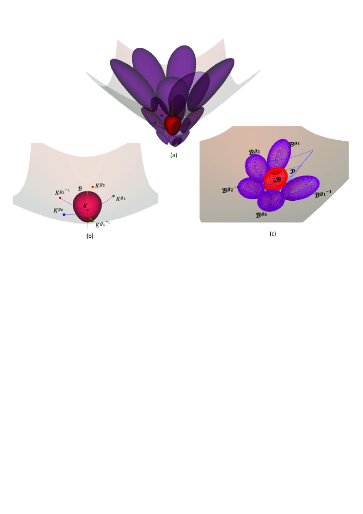
Figure 3: The optimal packing density configuration of simply transitive cases, $(2,5,4)$, with density $\delta^{opt}=0.53975\dots$. (a) The ”first neighbor crown’, (b) The ball and nearby orbit of the kernel, (c) The optimal ball, prism fundamental domain, and neighbor balls.

Using the above results, we obtain that

$$\frac{\partial\delta^{c}(\Gamma)}{\partial p_{k}}=-\frac{\pi}{{p_{k}}^{2}}\frac{\mathrm{vol}(\mathcal{D}(K))\left(\frac{\partial}{\partial\alpha_{k}}(\mathrm{vol}(\mathcal{B}(K)))\right)-\mathrm{vol}(\mathcal{B}(K))\left(\frac{\partial}{\partial\alpha_{k}}(\mathrm{vol}(\mathcal{D}(K))\right)}{(\mathrm{vol}(\mathcal{D}(K)))^{2}}<0.\leavevmode\nobreak\ \leavevmode\nobreak\ \leavevmode\nobreak\ \leavevmode\nobreak\ \square$$

Moreover, We provide some graphs of density functions in cases $(2,p_{1},3)$, $(2,p_{1},4)$, and $(2,p_{1},5)$, see Fig.4. These density functions $\delta$ are monotonically decreasing as parameter $p_{1}$ increases.

$(2,p_{1},p_{2})$	$\rho^{opt}$	$\mathrm{vol}({B})$	$\delta^{opt}$
$(2,7,3)$	$0.18773\dots$	$0.02777\dots$	$0.49454\dots$
$(2,8,3)$	$0.24309\dots$	$0.06040\dots$	$0.47451\dots$
$\vdots$	$\vdots$	$\vdots$	$\vdots$
$(2,12,3)$	$0.32328\dots$	$0.14251\dots$	$0.42095\dots$
$\vdots$	$\vdots$	$\vdots$	$\vdots$
$(2,20,3)$	$0.35904\dots$	$0.19555\dots$	$0.37149\dots$
$\vdots$	$\vdots$	$\vdots$	$\vdots$
$(2,p_{2}\rightarrow\infty,3)$	$0.37815\dots$	$0.22868\dots$	$0.28873\dots$

Table 1: $(2,p_{1},3)$ simply transitive ball packings

$(2,p_{1},p_{2})$	$\rho^{opt}$	$\mathrm{vol}({B})$	$\delta^{opt}$
$(2,5,4)$	$0.28377\dots$	$0.09623\dots$	$0.53975\dots$
$(2,6,4)$	$0.35877\dots$	$0.19510\dots$	$0.51930\dots$
$\vdots$	$\vdots$	$\vdots$	$\vdots$
$(2,12,4)$	$0.46847\dots$	$0.43700\dots$	$0.44539\dots$
$\vdots$	$\vdots$	$\vdots$	$\vdots$
$(2,20,4)$	$0.49033\dots$	$0.50176\dots$	$0.40716\dots$
$\vdots$	$\vdots$	$\vdots$	$\vdots$
$(2,p_{2}\rightarrow\infty,4)$	$0.50247\dots$	$0.54049\dots$	$0.31987\dots$

Table 2: $(2,p_{1},4)$ simply transitive ball packings

$(2,p_{1},p_{2})$	$\rho^{opt}$	$\mathrm{vol}({B})$	$\delta^{opt}$
$(2,5,5)$	$0.39445\dots$	$0.25977\dots$	$0.52406\dots$
$(2,6,5)$	$0.44772\dots$	$0.38100\dots$	$0.50788\dots$
$\vdots$	$\vdots$	$\vdots$	$\vdots$
$(2,12,5)$	$0.53359\dots$	$0.64858\dots$	$0.44642\dots$
$\vdots$	$\vdots$	$\vdots$	$\vdots$
$(2,20,5)$	$0.55148\dots$	$0.71693\dots$	$0.41380\dots$
$\vdots$	$\vdots$	$\vdots$	$\vdots$
$(2,p_{1}\rightarrow\infty,5)$	$0.56151\dots$	$0.75730\dots$	$0.35775\dots$

Table 3: $(2,p_{1},5)$ simply transitive ball packings

$(2,p_{1},p_{2})$	$\rho^{opt}$	$\mathrm{vol}({B})$	$\delta^{opt}$
$(2,p_{1}\rightarrow\infty,p_{2}\rightarrow\infty)$	$0.67122\dots$	$1.30530\dots$	$0.30950\dots$

Table 4: $(2,p_{1}\rightarrow\infty,p_{2}\rightarrow\infty)$ simply transitive ball packings

Using the results of the Theorem 4.1and the Lemma 4.2 we obtain the following

Theorem 4.3

The optimal packing density configuration of geodesic ball packings generated by rotations in simply transitive cases is realized with parameters $(2,5,4)$, where the optimal density is $\delta^{opt}=0.53975\dots$.

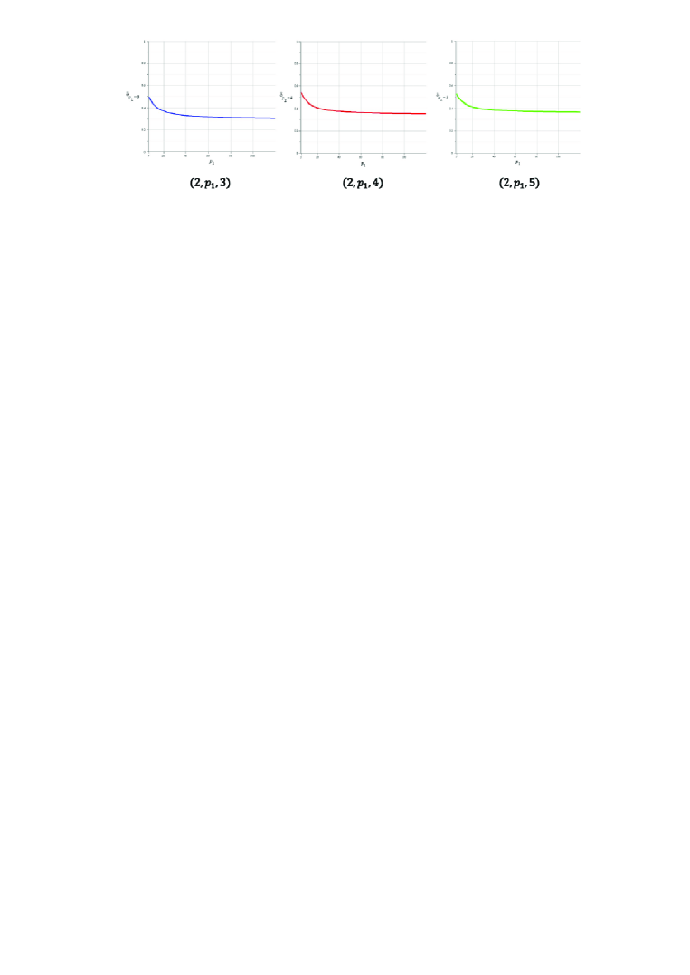
Figure 4: The monotonicity (decreasing) behaviour of density function $\delta^{opt}$ on simply transitive cases of $(2,p_{1},3),\leavevmode\nobreak\ (2,p_{1},4)$, and $\leavevmode\nobreak\ (2,p_{1},5)$

.

4.1.2 Optimal multiply transitive ball packings

We now consider a kernel point $K\in\mathbf{H}^{2}\times\mathbf{R}$ (on hyperbolic base plane) such that the stabilizer of $K$, $\Gamma_{K}\neq\mathbf{I}$. Then, it allows us to generate ball-packing $\mathcal{B}^{\Gamma}(K)$ and find the corresponding density $\delta(K)$ is maximal. In this multi-transitive case, we observe the optimal kernel $K$ in the closed triangular region $ABC$. In fact, we have three different cases i.e. where kernel point $K$ coincides with vertex $A,B$, or $C$.

Kernel point coincides with $A$.

If we choose $K$ at $A$, then $g_{0}$ is a stabilizer of $K$, see Fig. 3 (a). In that case, the optimum radius of the inscribed circle $\rho^{opt}$, will be $\rho^{opt}=\frac{1}{2}d(K,K^{g_{1}})=\frac{1}{2}d(K,K^{\mathbf{g}_{1}})=\frac{1}{2}d(K,K^{\mathbf{g}_{2}^{-1}})=\frac{1}{2}d(K,K^{\mathbf{g}_{1}^{-1}})=\frac{1}{2}d(K,K^{\mathbf{g}_{0}\mathbf{g}_{1}})$. On the other hand, the segment $BC$ is a part of the line bisector of $KK^{\mathbf{g}_{1}}$. Therefore, the maximum radius is equal to the distance between $A$ and the line $BC$ i.e.

$$\rho^{opt}=\sinh^{-1}\left(\frac{-\langle\mathbb{a},\boldsymbol{u}_{a}\rangle}{\sqrt{\langle\mathbb{a},\mathbb{a}\rangle\langle\boldsymbol{u}_{a},\boldsymbol{u}_{a}\rangle}}\right)$$

To compute the prism volume, we consider the circumscribing polygon, in this case the the area of the circumscribing polygon is $4\cdot\mathrm{area}(ABC)$. Hence the volume of the prism is

$$\mathrm{vol}(\mathcal{D}(K=A))=2\cdot\rho^{opt}\cdot 4\cdot\mathrm{area}(ABC)=8\cdot\rho^{opt}\cdot\left(\frac{\pi}{2}-\frac{\pi}{p_{1}}-\frac{\pi}{p_{2}}\right).$$

Figure 5: The structure of the orbit with centre $K$ in the hyperbolic base plane where $K$ coincides with $A$, $B$ or $C$, i.e. $\Gamma_{K}\neq\mathbf{I}$ and the optimal fundamental domain with inscribed circle in the base hyperbolic plane in multiply transitive cases.

Once have the volume of the ball and prism, we can immediately compute the packing density.

Kernel point coincides with $B$.

Analogously, we apply the previous method by choosing the kernel at point $B$. Therefore, $\mathbf{g}_{1}$ is the stabilizer of $K$, see Fig. 3 (b). Here, the optimum radius will equal the distance of points $B$ and $A$, i.e.$\rho=\cosh^{-1}\left(\frac{-\langle\mathbb{b},\mathbb{a}\rangle}{\sqrt{\langle\mathbb{b},\mathbb{b}\rangle\langle\mathbb{a},\mathbb{a}\rangle}}\right)$. On the hyperbolic base, a $p_{1}$-sided regular polygonal region is formed whose the area is $\mathrm{vol}(\mathcal{D}(K=B))=2\cdot\rho^{opt}\cdot 2\cdot p_{1}\cdot\mathrm{area}(ABC)=4\cdot p_{1}\cdot\rho^{opt}\cdot\left(\frac{\pi}{2}-\frac{\pi}{p_{1}}-\frac{\pi}{p_{2}}\right)$.

Kernel point coincides with $C$.

Again, by applying analogous method (see Fig. 3 (c)).
We know the optimal radius $\rho^{opt}=\cosh^{-1}\left(\frac{-\langle\mathbb{a},\mathbb{c}\rangle}{\sqrt{\langle\mathbb{a},\mathbb{a}\rangle\langle\mathbb{c},\mathbb{c}\rangle}}\right)$, and $C$ is surrounded by $p_{2}$-regular prisms whose volume is given by $\mathrm{vol}(\mathcal{D}(K=C))=2\cdot\rho^{opt}\cdot 2\cdot p_{2}\cdot\mathrm{area}(ABC)=4\cdot p_{2}\cdot\rho^{opt}\cdot\left(\frac{\pi}{2}-\frac{\pi}{p_{1}}-\frac{\pi}{p_{2}}\right)$.
Hence for every $(p_{0},p_{1},p_{2})$ we have 3 different cases. We need to determine the optimum among these cases. The following table is the example $(2,8,3)$.

Kernel point	$\rho^{opt}$	$\mathrm{vol}(\mathcal{B})$	$\delta^{opt}$
A	$0.31648\dots$	$0.13367\dots$	$0.40333\dots$
B	$0.76428\dots$	$1.94411\dots$	$0.60726\dots$
C	$0.36351\dots$	$0.20300\dots$	$0.35550\dots$

Table 5: Multi transitive case: The computation result of radius, ball volume, and density in case of $(2,8,3)$ from various kernel points.

$(p_{0},p_{1},p_{2})$	Opt.Kernel point	$\rho^{opt}$	$\mathrm{vol}(\mathcal{B}(K))$	$\delta^{opt}$
$(2,7,3)$	$B$	$0.54527\dots$	$0.69267\dots$	$0.60653\dots$
$(2,8,3)$	$B$	$0.76428\dots$	$1.94411\dots$	$0.607262\dots$
$(2,9,3)$	$B$	$0.92753\dots$	$3.53909\dots$	0.607267…
$(2,10,3)$	$B$	$1.06127\dots$	$5.39521\dots$	$0.60682\dots$
$(2,11,3)$	$B$	$1.17585\dots$	$7.46309\dots$	$0.60608\dots$
$(2,12,3)$	$B$	$1.27668\dots$	$9.70891\dots$	$0.60516\dots$
$\vdots$	$\vdots$	$\vdots$	$\vdots$	$\vdots$
$(2,20,3)$	$B$	$1.82969\dots$	$31.96254\dots$	$0.59576\dots$
$\vdots$	$\vdots$	$\vdots$	$\vdots$	$\vdots$
$(2,p_{1}\rightarrow\infty,3)$	$A$	$0.48121\dots$	$0.47401\dots$	$0.23516\dots$

Table 6: Multi transitive cases $(2,p_{1},3)$: The local maximum density is attained at $(2,9,3)$ with density $\delta^{opt}=0.607267\dots$

$(p_{0},p_{1},p_{2})$	Opt. Kernel point	$\rho^{opt}$	$\mathrm{vol}(\mathcal{B}(K))$	$\delta^{opt}$
$(2,5,4)$	$B$	$0.62686\dots$	$1.05919\dots$	$0.53783\dots$
$(2,6,4)$	$B$	$0.88137\dots$	$3.01979\dots$	$0.54530\dots$
$(2,7,4)$	$B$	$1.07040\dots$	$5.54276\dots$	$0.54942\dots$
$(2,8,4)$	$B$	$1.22422\dots$	$8.48710\dots$	$0.55168\dots$
$(2,9,4)$	$B$	$1.35504\dots$	$11.76673\dots$	$0.55281\dots$
$(2,10,4)$	$B$	$1.46935\dots$	$15.32291\dots$	$\mathbb{0.55324\dots}$
$(2,11,4)$	$B$	$1.57108\dots$	$19.11300\dots$	$0.55319\dots$
$(2,12,4)$	$B$	$1.66288\dots$	$23.10472\dots$	$0.55283\dots$
$\vdots$	$\vdots$	$\vdots$	$\vdots$	$\vdots$
$(2,20,4)$	$B$	$2.18922\dots$	$60.06928\dots$	$0.54587\dots$
$\vdots$	$\vdots$	$\vdots$	$\vdots$	$\vdots$
$(2,p_{1}\rightarrow\infty,4)$	$A$	$0.65847\dots$	$1.23095\dots$	$0.29752\dots$

Table 7: Multi transitive cases $(2,p_{1},4)$: The local maximum density is attained at $(2,10,4)$ with density $\delta^{opt}=0.55324\dots$

$(p_{0},p_{1},p_{2})$	Opt. Kernel point	$\rho^{opt}$	$\mathrm{vol}(\mathcal{B}(K))$	$\delta^{opt}$
$(2,5,5)$	$B$	$0.84248\dots$	$2.62573\dots$	$0.49603\dots$
$(2,6,5)$	$B$	$1.06127\dots$	$5.39521\dots$	$0.50568\dots$
$\vdots$	$\vdots$	$\vdots$	$\vdots$	$\vdots$
$(2,10,5)$	$B$	$1.61692\dots$	$21.03412\dots$	$0.51760\dots$
$(2,11,5)$	$B$	$1.71621\dots$	$25.69831\dots$	$0.51807\dots$
$(2,12,5)$	$B$	$1.80620\dots$	$30.57818\dots$	$\mathbb{0.51815\dots}$
$(2,13,5)$	$B$	$1.88855\dots$	$35.64729\dots$	$0.51795\dots$
$(2,14,5)$	$B$	$1.96447\dots$	$40.88437\dots$	$0.51754\dots$
$\vdots$	$\vdots$	$\vdots$	$\vdots$	$\vdots$
$(2,20,5)$	$B$	$2.32684\dots$	$75.03233\dots$	$0.51321\dots$
$\vdots$	$\vdots$	$\vdots$	$\vdots$	$\vdots$
$(2,p_{1}\rightarrow\infty,5)$	$A$	$0.73969\dots$	$1.75810\dots$	$0.31523\dots$

Table 8: Multi transitive cases $(2,p_{1},5)$: The local maximum density is attained at $(2,12,5)$ with density $\delta^{opt}=0.51815\dots$

$(p_{0},p_{1},p_{2})$	Opt.Kernel point	$\rho^{opt}$	$\mathrm{vol}(\mathcal{B}(K))$	$\delta^{opt}$
$(2,p_{1}\rightarrow\infty,p_{2}\rightarrow\infty)$	$A$	$0.88137\dots$	$3.01979\dots$	$0.27265\dots$

Table 9: Multi transitive cases $(2,p_{1}\rightarrow\infty,p_{2}\rightarrow\infty)$ with density $\delta^{opt}=0.27265\dots$

We do not discuss the monotonic properties of densities separately here, but it can be done similarly to Lemma 4.2. Finally, we obtain the following

Theorem 4.4

The optimal packing density configuration of geodesic ball packings generated by rotations in multiply transitive cases is realized with parameters $(2,9,3)$, where the optimal ball centred at vertex $B$ and the optimal density is $\delta^{opt}=0.607267\dots$.

Remark 4.5

1. The density of the densest multiply transitive ball packings and its configuration is the same as the density and the structure of the known densest ball packing belonging to the generalized Coxeter groups $(3,3,3,3,3,3,3,3,3)$ in $\mathbf{H}^{2}\!\times\!\mathbf{R}$ space (see [25]).

2. If we choose a kernel point $K$, which coincides with $B$, and take the parameters $(2,p_{1}\rightarrow\infty,3)$ then the corresponding Dirichlet-Voronoi cell is a prism centred at $B$ lying at infinity and the “ball” will be a horospherical cylinder. Their packing density is $3/\pi\approx 0.945$ which is equal to the density to the densest circle packing in the hyperbolic plane. However, this case cannot be classified as one of the studied ball packings, because it is not a continuous extension of the cases of ball packings. This case belongs to the topic of cylinder packings, which were also examined in the paper [38] in both the $\mathbf{H}^{2}\!\times\!\mathbf{R}$ and $\widetilde{\mathbf{S}\mathbf{L}_{2}\mathbf{R}}$S spaces.

In this paper, we mentioned only some natural problems related to $\mathbf{H}^{2}\!\times\!\mathbf{R}$ space, but we hope that from these the reader can appreciate that our projective method is suitable to study and solve similar problems that represent a huge class of open mathematical problems (see e.g. [7], [8], [10], [13], [16], [30], [12], [14], [11], [34], [28], [27]). Detailed studies are the objective of ongoing research.

5 Appendix

5.1 The explicit solution of system of equation (4.4) for optimal radius and koordinates of centre of optimal ball in simply transitive cases

The system (4.4) can be reduced into 2 explicit expressions for $\rho^{opt},\leavevmode\nobreak\ k_{1}$ and 1 fourth-degree polynomial of $k_{2}$ with explicit coefficient in term of $p_{1},p_{2}$, as follows:

$$\rho^{opt} =\operatorname{arccosh}{\left(\frac{k_{2}\sqrt{\cos^{2}{\frac{\pi}{p_{{1}}}}-\sin^{2}{\frac{\pi}{p_{{2}}}}}+\cos\frac{\pi}{p_{1}}}{\sin\frac{\pi}{p_{2}}\sqrt{1-k_{1}^{2}-k_{2}^{2}}}\right)}$$

$$k_{1} =\frac{\sqrt{\left(\sin^{4}\frac{\pi}{p_{2}}-\cos^{2}\frac{\pi}{p_{1}}\right)k_{2}^{2}-2\cos\frac{\pi}{p_{1}}\sqrt{\cos^{2}{\frac{\pi}{p_{{1}}}}-\sin^{2}{\frac{\pi}{p_{{2}}}}}k_{2}-\left(\cos^{2}{\frac{\pi}{p_{{1}}}}-\sin^{2}{\frac{\pi}{p_{{2}}}}\right)}}{\cos\frac{\pi}{p_{2}}\sin\frac{\pi}{p_{2}}}$$

$$a\leavevmode\nobreak\ k_{2}^{4}+b\leavevmode\nobreak\ k_{2}^{3}+c\leavevmode\nobreak\ k_{2}^{2}+d\leavevmode\nobreak\ k_{2}+e=0,$$

where the coefficients $a,b,c,d,e$ are given by

$$a =\left[\frac{1}{4}-\cos^{6}{\frac{\pi}{p_{{2}}}}+\left(\cos^{2}{\frac{\pi}{p_{{1}}}}+\frac{9}{4}\right)\cos^{4}{\frac{\pi}{p_{{2}}}}-\frac{3}{2}\cos^{2}{\frac{\pi}{p_{{2}}}}\right]\left[\cos^{2}{\frac{\pi}{p_{{1}}}}-\sin^{2}{\frac{\pi}{p_{{2}}}}\right]$$

$$b =\left[1-\cos^{6}{\frac{\pi}{p_{{2}}}}+\left(5+4\cos^{2}{\frac{\pi}{p_{{1}}}}\right)\,\cos^{4}{\frac{\pi}{p_{{2}}}}-5\cos^{2}{\frac{\pi}{p_{{2}}}}\right]\cos{\frac{\pi}{p_{{1}}}}\sqrt{\cos^{2}{\frac{\pi}{p_{{1}}}}-\sin^{2}{\frac{\pi}{p_{{2}}}}}$$

$$c =\left(3\,\cos^{2}{\frac{\pi}{p_{{1}}}}+\frac{3}{2}\right)\cos^{6}{\frac{\pi}{p_{{2}}}}+\,\left(6\,\cos^{4}{\frac{\pi}{p_{{1}}}}+\frac{3}{2}\,\cos^{2}{\frac{\pi}{p_{{1}}}}-\frac{7}{2}\right)\cos^{4}{\frac{\pi}{p_{{2}}}}$$

$$\leavevmode\nobreak\ +\,\left(\frac{5}{2}-6\,\cos^{2}{\frac{\pi}{p_{{1}}}}\right)\cos^{2}{\frac{\pi}{p_{{2}}}}+\frac{3}{2}\,\cos^{2}{\frac{\pi}{p_{{1}}}}-\frac{1}{2}$$

$$d =\left[1+\cos^{6}{\frac{\pi}{p_{{2}}}}+\left(1+4\,\cos^{2}{\frac{\pi}{p_{{1}}}}\right)\cos^{4}{\frac{\pi}{p_{{2}}}}-3\,\cos^{2}{\frac{\pi}{p_{{2}}}}\right]\cos{\frac{\pi}{p_{{1}}}}\sqrt{\cos^{2}{\frac{\pi}{p_{{1}}}}-\sin^{2}{\frac{\pi}{p_{{2}}}}}$$

$$e =\left[\left(\frac{1}{4}+\cos^{2}{\frac{\pi}{p_{{1}}}}\right)\cos^{4}{\frac{\pi}{p_{{2}}}}-\frac{1}{2}\,\cos^{2}{\frac{\pi}{p_{{2}}}}+\frac{1}{4}\right]\left[\cos^{2}{\frac{\pi}{p_{{1}}}}-\sin^{2}{\frac{\pi}{p_{{2}}}}\right].$$

Once we have the solution $k_{2}$ in the polynomial, the values $k_{1}$ and radius $\rho^{opt}$ are easily computed.
Based on our setting, we have to choose the real negative root $k_{2}$, For all $p_{1},p_{2}$ that satisfy $\frac{1}{p_{1}}+\frac{1}{p_{2}}<\frac{1}{2}$. Since any fourth-degree polynomial can be solved by radicals (while the fifth and higher degree can not be solved in this way i.e. Abel Ruffini Theorem), then we can formulate the exact negative real values of $k_{2}$.

$$\begin{gathered}k_{2}=-\frac{b}{4a}+S+\frac{1}{2}\sqrt{-4S^{2}-2p-\frac{q}{S}},\leavevmode\nobreak\ \text{where}\leavevmode\nobreak\ S=\frac{1}{2}\sqrt{-\frac{2}{3}p+\frac{1}{3a}(Q+\frac{\Delta_{0}}{Q})}\leavevmode\nobreak\ \text{and}\\ q=\frac{b^{3}-4abc+8a^{2}d}{8a^{3}},\leavevmode\nobreak\ \text{with}\leavevmode\nobreak\ p=\frac{8ac-3b^{2}}{8a^{2}},\leavevmode\nobreak\ Q=\sqrt[3]{\frac{\Delta_{1}+\sqrt{\Delta_{1}^{2}-4\Delta_{0}^{3}}}{2}},\\ \Delta_{1}=2c^{3}-9bcd+27ad^{2}+27b^{2}e-72ace,\leavevmode\nobreak\ \Delta_{0}=c^{2}-3bd+12ae.\end{gathered}$$

We do not provide directly the complete expression of $k_{2}$ due to the large size of the full expression.

References

- [1] Farkas, Z. J. The classification of space groups, Beitr. Algebra Geom., 42 (2001), 235–250.
- [2] Fejes Tóth, G. - Kuperberg, W. Packing and Covering with Convex Sets, Handbook of Convex Geometry Volume B, eds. Gruber, P.M., Willis J.M., pp. 799-860, North-Holland, (1983).
- [3] Fejes Tóth, L. — Fejes Tóth, G. — Kuperberg, W. Lagerungen: Arrangements in the Plane, on the Sphere, and in Space 360 Grundlehren der mathematischen Wissenschaften Springer Nature, (2023), ISBN 3031218000, 9783031218002.
- [4] Fejes Tóth, L. Regular Figures, Macmillan (New York), 1964.
- [5] Macbeath, A. M The classification of non-Euclidean plane crystallographic groups. Can. J. Math., 19 (1967), 1192–1205.
- [6] Molnár, E. The projective interpretation of the eight 3-dimensional homogeneous geometries. Beitr. Algebra Geom., 38 No. 2 (1977), 261–288.
- [7] Molnár, E. — Szirmai, J. Symmetries in the 8 homogeneous 3-geometries. Symmetry Cult. Sci., 21/1-3 (2010), 87–117.
- [8] Molnár, E. — Szirmai, J. Top dense hyperbolic ball packings and coverings for complete Coxeter orthoscheme groups, Publications de l’Institut Mathématique, 103(117) (2018), 129–146, DOI: 10.2298/PIM1817129M.
- [9] Molnár, E. — Szirmai, J. Classification of lattices. Geom. Dedicata, 161/1 (2012), 251-275.
- [10] Molnár E. — Szirmai J. — Vesnin A., Geodesic and Translation Ball Packings Generated by Prismatic Tesselations of the Universal Cover of , Results in Math. 71) (2017) 623–642.
- [11] Molnár, E. – Szirmai, J. Volumes and geodesic ball packings to the regular prism tilings in space. Publ. Math. Debrecen, 84/1-2 (2014), 189-203, DOI: 10.5486/PMD.2014.5832.
- [12] Molnár, E. – Szirmai, J. On homogeneous 3-geometries, balls and their optimal arrangements, especially in and spaces. G-Slovak Journal for Geometry and Graphics 19 (2022), 37, 5-32.
- [13] Molnár, E. — Szirmai, J. Packings with geodesic and translation balls and their visualizations in space. Journal for Geometry and Graphics 26(1) (2022), 51–64.
- [14] Molnár, E. – Szirmai, J. – Vesnin, A. Projective metric realizations of cone-manifolds with singularities along 2-bridge knots and links. J. Geometry, 95 (2009), 91-133.
- [15] Molnár, E. – Szirmai, J. – Vesnin, A. Packings by translation balls in . J. Geometry, 105 (2) (2014), 287-306, DOI: 10.1007/s00022-013-0207-x.
- [16] Németh, L. Pascal pyramid in the space . Mathematical Communications 22 (2017), 211–225.
- [17] Pallagi, J. — Schultz, B. — Szirmai, J. Visualization of geodesic curves, spheres and equidistant surfaces in space. KoG, 14 (2010), 35–40.
- [18] Pallagi, J. — Schultz, B. — Szirmai, J. Equidistant surfaces in space. KoG, 15, (2011), 3-6.
- [19] Pallagi, J. — Szirmai, J. Visualization of the Dirichlet-Voronoi cells in space. Pollack Periodica, 7 Supp 1, 95–104 (2012), DOI: 10.1556/Pollack.7.2012.S.9.
- [20] Scott, P. The geometries of 3-manifolds. Bull. London Math. Soc. 15 (1983), 401–487.
- [21] Szirmai, J. The densest geodesic ball packing by a type of lattices. Beitr. Algebra Geom. 48(2) (2007), 383–398.
- [22] Szirmai, J. A candidate to the densest packing with equal balls in the Thurston geometries. Beitr. Algebra Geom., 55(2) (2014), 441–452.
- [23] Szirmai, J. Simply transitive geodesic ball packings to space groups generated by glide reflections, Ann. Mat. Pur. Appl., 193/4 (2014), 1201-1211, DOI: 10.1007/s10231-013-0324-z.
- [24] Szirmai, J. Geodesic ball packings in space for generalized Coxeter space groups. Beitr. Algebra Geom., 52, (2011), 413 – 430.
- [25] Szirmai, J. Geodesic ball packings in space for generalized Coxeter space groups. Math. Commun., 17/1 (2012), 151–170.
- [26] Szirmai, J. Interior angle sums of geodesic triangles in and geometries. Bul. Acad. de Stiinte Republicii Mold. Mat., 93(2) (2020), 44–61.
- [27] Szirmai, J. Apollonius surfaces, circumscribed spheres of tetrahedra, Menelaus’ and Ceva’s theorems in and geometries. Q. J. Math., (2021), DOI: 10.1093/qmath/haab038.
- [28] Szirmai, J. On Menelaus’ and Ceva’s theorem in geometry. Acta Univ. Sapientiae, Mathematica, 15, 1 (2023), 155-173, DOI: 10.2478/ausm-2023-0010.
- [29] Szirmai, J. Hyperball packings in hyperbolic -space, Mat. Vesn., 70/3 (2018), 211–221.
- [30] Szirmai, J Non-periodic geodesic ball packings to infinite regular prism tilings in space. Rocky Mountain J. Math. 46/3 (2016), 1055–1070.
- [31] Szirmai, J. Packings with horo- and hyperballs generated by simple frustum orthoschemes, Acta Math. Hungar., 152/2 (2017), 365–382, DOI:10.1007/s10474-017-0728-0.
- [32] Szirmai, J. The -gonal prism tilings and their optimal hypersphere packings in the hyperbolic 3-space, Acta Math. Hungar., 111 (1-2) (2006), 65–76.
- [33] Szirmai, J. The regular prism tilings and their optimal hyperball packings in the hyperbolic -space, Publ. Math. Debrecen, 69 (1-2) (2006), 195–207.
- [34] Szirmai, J. A candidate to the densest packing with equal balls in the Thurston geometries. Beitr. Algebra Geom., (2013), DOI 10.1007/s13366-013-0158-2.
- [35] Szirmai, J. The optimal hyperball packings related to the smallest compact arithmetic -orbifolds, Kragujevac J. Math. 40(2) (2016), 260-270, DOI:10.5937/KgJMath1602260S.
- [36] Szirmai, J. The least dense hyperball covering to the regular prism tilings in the hyperbolic -space, Ann. Mat. Pur. Appl. 195/1 (2016), 235–248, DOI: 10.1007/s10231-014-0460-0.
- [37] Szirmai, J. Classical Notions and Problems in Thurston Geometries, Int. Electron. J. Geom. 16(2) (2023), 608-643, DOI: 10.36890/iejg.1221802.
- [38] Szirmai, J.: Fibre-like cylinders, their packings and coverings in space, Submitted manuscript (2023), arXiv: 2306.05721.
- [39] Thurston, W. P. (and Levy, S. editor), Three-Dimensional Geometry and Topology. Princeton University Press, Princeton, New Jersey, vol. 1 (1997).
- [40] Weeks, J. R. Real-time animation in hyperbolic, spherical, and product geometries. A. Prékopa and E. Molnár, (eds.). Non-Euclidean Geometries, János Bolyai Memorial Volume, Mathematics and Its Applications, Springer (2006) Vol. 581, 287–305.