Sensitivity analysis with multiple treatments and multiple outcomes with applications to air pollution mixtures

Abstract

Understanding the health impacts of air pollution is vital in public health research. Numerous studies have estimated negative health effects of a variety of pollutants, but accurately gauging these impacts remains challenging due to the potential for unmeasured confounding bias that is ubiquitous in observational studies. In this study, we develop a framework for sensitivity analysis in settings with both multiple treatments and multiple outcomes simultaneously. This setting is of particular interest because one can identify the strength of association between the unmeasured confounders and both the treatment and outcome, under a factor confounding assumption. This provides informative bounds on the causal effect leading to partial identification regions for the effects of multivariate treatments that account for the maximum possible bias from unmeasured confounding. We also show that when negative controls are available, we are able to refine the partial identification regions substantially, and in certain cases, even identify the causal effect in the presence of unmeasured confounding. We derive partial identification regions for general estimands in this setting, and develop a novel computational approach to finding these regions.

Keywords: Causal inference, Sensitivity analysis, Multiple treatments, Multiple Outcomes, Environmental mixtures.

1 Introduction

Understanding the health effects of air pollution is a critically important problem in public health research. There is a vast literature studying associations between air pollutants and a variety of health outcomes that indicate substantial detrimental impacts of air pollution (Dockery et al., 1993; Pope Iii et al., 2002; Cohen et al., 2017; Burnett et al., 2018; Manisalidis et al., 2020). This has helped inform regulatory policy on how to reduce air pollution, and it is important to obtain accurate estimates of the impact of these policies as both the costs and benefits of these policies are in the billions of dollars (Portney, 1990). Due to the importance of this problem and the need for policy-relevant estimates of the impacts of air pollution, there has been a push towards causal inference approaches in environmental epidemiology (Dominici & Zigler, 2017; Carone et al., 2020; Sommer et al., 2021). Causal inference in these settings is difficult for a multitude of reasons, but arguably the biggest impediment to assessing the causal effect of environmental exposures is the potential for unmeasured confounding bias. In some settings, a natural experiment is available that helps to alleviate issues stemming from unmeasured confounding (Rich, 2017). Examples include pollution reductions due to the Olympic games in Atlanta or Beijing (Huang et al., 2015) or the decommissioning of power plants leading to large reductions in pollution for nearby areas (Luechinger, 2014). Other work has looked to leverage recent advancements in double negative control designs to estimate causal effects in a manner that is robust to unmeasured confounding (Schwartz et al., 2023). Generally, however, these approaches are not always available. In such cases, sensitivity analysis should be utilized, though very little work has been done to assess the robustness of findings to potential bias from unmeasured confounding.

Sensitivity analysis for causal effects dates back at least as far as Cornfield et al. (1959) who utilized sensitivity analysis in observational studies to argue for a causal relationship between smoking and lung cancer. A central goal of sensitivity analysis is to provide bounds on the causal effect that account for biases stemming from unmeasured confounding. In simple cases such as with bounded outcomes, general bounds for causal effects can be estimated (Manski, 1990), though typically bounds are in terms of sensitivity parameters governing the strength of association between the unmeasured confounder and either the treatment or outcome. One approach is to posit a sensitivity parameter for the relationship between the unmeasured variable and treatment, while assuming the worst-case scenario that the unmeasured variable and outcome are nearly co-linear (Rosenbaum, 1987, 1988, 1991, 2002b, 2002a). Other approaches have two sensitivity parameters that govern the strength of association between the unmeasured variable and both the treatment and outcome. These parameters are intended to be interpretable so that one can reason about potential values for them. This can be done by letting them be parameters of a regression model (Rosenbaum & Rubin, 1983; McCandless et al., 2007), parameters dictating relative risks (VanderWeele & Ding, 2017; Ding & VanderWeele, 2016a), or partial $R^{2}$ values between the unmeasured variable and the treatment or outcome (Imbens, 2003; Small, 2007; Veitch & Zaveri, 2020; Cinelli & Hazlett, 2020; Freidling & Zhao, 2022; Chernozhukov et al., 2022). Additionally, while much of this work has focused on average treatment effects for binary treatments, similar ideas have been extended to situations such as mediation (Imai et al., 2010; VanderWeele, 2010; Ding & Vanderweele, 2016b; Zhang & Ding, 2022), among others.

While much of the existing work focuses on a single treatment variable, recent work has examined settings with multiple treatments (Miao et al., 2022; Kong et al., 2022; Zheng et al., 2021, 2022). Under certain assumptions about the nature of the measured confounder, partial $R^{2}$ values between the unmeasured confounders and treatment can be identified from the observed data. In some cases, such as sparsity in the effects of the treatment on the outcome, the causal effects are even identifiable in this setting (Miao et al., 2022). Similar benefits have been seen in the multi-outcome setting, where partial $R^{2}$ values between the unmeasured confounder and outcome can be estimated from the observed data in the absence of data on the unmeasured confounder (Zheng et al., 2023). These lead to more informative sensitivity analyses, because some of the sensitivity parameters are identified by the observed data, and more information on the degree of potential confounding bias is available.

In this paper, we develop a sensitivity analysis framework for scenarios with both multiple treatments and multiple outcomes. We demonstrate that leveraging information from multiple treatments and outcomes can provide informative bounds on causal effects that account for potential bias from unmeasured confounding, and these bounds can be tighter than those from single treatment or single outcome studies. We show that under certain factor confounding assumptions, the partial $R^{2}$ between the unmeasured confounders and both the treatment and outcome can be identified, which leads to a bound on the causal effect that accounts for the worst case scenario bias given the estimated associations with the unmeasured variable. We also derive partial identification regions for when a negative control treatment or outcome is available. These bounds highlight when negative controls are most useful in terms of reducing the width of the partial identification region, which provides practitioners with guidance for how to select negative controls for their study. Additionally, these results highlight that in certain situations, negative controls can be incorporated to identify the causal effect in the presence of unmeasured confounding. Additionally, we develop a computational strategy to finding the partial identification regions numerically, which can provide additional insights into possible values of the causal effect of interest beyond what the theoretical intervals provide.

2 Notation and estimands

Throughout, we observe $(Y_{i},T_{i},X_{i})$ for $i=1,\dots,n$. Here, $T=(T_{1},\cdots,T_{k})^{\top}$ denotes a vector of $k$ treatments, $Y=(Y_{1},\cdots,Y_{q})^{\top}$ denotes a vector of $q$ outcomes, and $X=(X_{1},\cdots,X_{l})^{\top}$ denotes a vector of $l$ pre-treatment covariates, respectively. Under the potential outcome framework (Splawa-Neyman et al., 1990; Rubin, 1974), we let $Y(t)$ denote the potential outcome that would have been observed had the treatment $T$ been set to $t$. Our goal throughout will be to utilize the observed data to estimate the population average treatment effect (PATE), for any linear combinations of outcomes $a^{\top}Y$, defined as

$$\text{PATE}_{a,t_{1},t_{2}}:=E[a^{\top}Y(t_{1})-a^{\top}Y(t_{2})]$$

for some $t_{1},t_{2}$. If unmeasured confounders $U$ were observed along with $X$, we could identify the causal effect from the observed data under the following assumptions:

Assumption 1 (SUTVA; Stable Unit Treatment Value Assumption).

There is no interference between units and there is only a single version of each assigned treatment.

Assumption 2 (Latent ignorability).

$Y(t)\perp\!\!\!\perp T\mid(U,X)$ for all $t$.

Assumption 3 (Latent positivity).

$f(t\mid U=u,X=x)>0$ for all possible values of $t$, $x$, and $u$. Here, $f(\cdot)$ represents the conditional density function of $T$ given $(X,U)$.

Assumption 1 ensures that $Y(t)$ is well-defined and that $Y=Y(t)$ if $T=t$, which links the observed data to potential outcomes. Assumption 2 states that $X$ and $U$ contain all common causes of $T$ and $Y$. Under this assumption, we can identify the causal effect of interest using $E[Y(t)]=E_{X,U}[E(Y|T=t,X,U)]$. Assumption 3, also referred to as overlap, assures that there is a positive probability that each unit receives any treatment value $t$ given both $X$ and $U$.

Note that our identification assumptions include unmeasured confounders $U$, which are not observed, and therefore the causal effect is not identifiable without further assumptions, as the effect of $T$ on $Y$ may be confounded by $U$ even after conditioning on $X$. Our goal in this manuscript is to provide sensitivity analysis and derive bounds for the causal effect that account for the potential presence of unmeasured confounders when we have both multiple treatments and multiple outcomes under varying assumptions about the unmeasured variables. At first, we assume the number of unmeasured confounders $m$ is known and fixed as in previous works. We discuss estimation of $m$ in Section 4 and evaluate how this choice impacts results in Section 5.

3 Partial Identification and Sensitivity Analysis

In this section, we first show that the causal effect of interest is not point-identified in our setting, but the range of possible values for the causal effect can be characterized by sensitivity parameters that, under a factor confounding assumption that we detail in subsequent sections, can be identified in the multi-treatment and multi-outcome setting. We also derive results showing how negative control treatments or outcomes can reduce the widths of the bounds on the causal effect, and can even identify the causal effect of interest in certain settings. We also develop an optimization algorithm for finding negative control bounds on causal effects that is, at times, more informative than analytic results.

3.1 Factor models with multivariate treatment and outcome

For ease of exposition, we do not include observed covariates $X$ in this section, though all results hold analogously when conditioning on $X$. Throughout, we consider the following latent variable models for the observed and unobserved data:

$$U =\epsilon_{U},~{}~{}~{}$$ (1)

$$T =BU+\epsilon_{T},~{}~{}~{}$$ (2)

$$Y =g(T)+\Gamma\Sigma_{u|t}^{-1/2}U+\epsilon_{Y},~{}~{}~{}$$ (3)

where $B\in\mathbb{R}^{k\times m}$, $\Gamma\in\mathbb{R}^{q\times m}$, and $\Sigma_{u|t}:=\text{Cov}(U|T=t)$. We let $\epsilon_{U}\sim N_{m}(0,I_{m})$, $\epsilon_{T}\sim N_{k}(0,\Sigma_{t|u})$, and $\epsilon_{Y}\sim N_{q}(0,\Sigma_{y|t,u})$. We assume that $\epsilon_{Y}\perp\!\!\!\perp T,U$. From (1)–(2), the conditional confounder distribution can be derived as

$$f(u|T=t)\sim N_{m}(\mu_{u|t},\Sigma_{u|t})$$ (4)

where

$$\mu_{u|t} =B^{\top}(BB^{\top}+\Sigma_{t|u})^{-1}t,$$

$$\Sigma_{u|t} =I_{m}-B^{\top}(BB^{\top}+\Sigma_{t|u})^{-1}B.$$

Under the models (1)–(3), the potential outcome distribution has density

$$f\{Y(t)=y\}\sim N_{q}(g(t),\Gamma\Gamma^{\top}+\Sigma_{y|t,u}).$$

Our interest is to estimate $E[Y(t)]$, which is parameterized by the function $g$, which we want to recover from the observed data. The observed outcome distribution can be written as

$$f(y|T=t)\sim N_{q}(\check{g}(t),\Sigma_{y|t})$$

where the observed mean and covariance are expressed as

$$\check{g}(t) =g(t)+\Gamma\Sigma_{u|t}^{-1/2}\mu_{u|t},$$

$$\Sigma_{y|t} =\Gamma\Gamma^{\top}+\Sigma_{y|t,u}.$$ (5)

Then, our estimand of interest and its corresponding bias when ignoring $U$ can be expressed as

$$\text{PATE}_{a,t_{1},t_{2}} :=E[a^{\top}Y(t_{1})-a^{\top}Y(t_{2})]$$ (6)

$$=a^{\top}g(t_{1})-a^{\top}g(t_{2})$$ (7)

and

$$\text{Bias}_{a,t_{1},t_{2}} =[a^{\top}\check{g}(t_{1})-a^{\top}\check{g}(t_{2})]-\text{PATE}_{a,t_{1},t_{2}}$$

$$=a^{\top}\Gamma\Sigma_{u|t}^{-1/2}\mu_{u|\Delta t},$$ (8)

where $\mu_{u|\Delta t}=\mu_{u|t_{1}}-\mu_{u|t_{2}}$.

3.2 Bound of confounding bias

While the bias term in equation (3.1) is not identifiable in the absence of data on $U$, we can derive upper bounds for this bias that are themselves identifiable under certain assumptions about the unmeasured confounders.

Theorem 1.

Assuming models (1)–(3), the confounding bias of $\text{PATE}_{a,t_{1},t_{2}}$ can be bounded as

$$\text{Bias}_{a,t_{1},t_{2}}^{2}\leq\|a^{\top}\Gamma\|_{2}^{2}\|\Sigma_{u|t}^{-1/2}\mu_{u|\Delta t}\|^{2}_{2},$$

where the right-hand side is the worst-case bias of the naive estimator and is achieved when $a^{\top}\Gamma$ is colinear with $\Sigma_{u|t}^{-1/2}\mu_{u|\Delta t}$.

The proof of the theorem is given in Appendix A.1. $a^{\top}\Gamma$ can be viewed as the strength of association between the unmeasured variables $U$ and the outcome, while $\Sigma_{u|t}^{-1/2}\mu_{u|\Delta t}$ is the scaled difference in unmeasured confounder means when treatment is shifted from $t_{1}$ to $t_{2}$ and represents the strength of association between the unmeasured confounders and treatment. This result implies that the true treatment effect lies in the interval

$$a^{\top}[\check{g}(t_{1})-\check{g}(t_{2})]\pm\|a^{\top}\Gamma\|_{2}\|\Sigma_{u|t}^{-1/2}\mu_{u|\Delta t}\|_{2},$$ (9)

which is the partial identification region for the PATE and is centered at the naively estimated PATE. While the confounding bias itself is not identifiable, it can be shown that this bound is identified under an assumption on the unmeasured confounders, which we detail in the following assumption.

Assumption 4 (Factor confounding assumption).

The data is generated by (1)–(3) and $U$ represents potential confounders in the sense that they are possible causes of $T$ and $Y$ and are not themselves caused by $T$ or $Y$. Additionally, we assume the following conditions are satisfied.

1. If any row of $\Gamma$ is deleted, there remain two disjoint submatrices of rank $m$, where $m=\text{rank}(\Gamma)$

2. If any row of $B$ is deleted, there remain two disjoint submatrices of rank $m$, where $m=\text{rank}(B)$.

We show in Appendix A.2 that the bias bound in equation (9) is identified under Assumption 4. Specifically, we show that $\|a^{\top}\Gamma\|_{2}^{2}$ is identified under condition (C1) and $\|\Sigma_{u|t}^{-1/2}\mu_{u|\Delta t}\|^{2}_{2}$ is identified under condition (C1). At the core of this result is that the factor loadings $\Gamma$ and $B$ are identifiable, but only up to certain matrix rotations. Implicit in the assumption above is that in order for $\Gamma$ to be identified up to rotation, we require that each confounder is correlated with at least three outcomes, and that $(q-m)^{2}-q-m\geq 0$, where $q$ is the number of outcomes in the data and $m$ is the number of unobserved confounders. Similarly, for $B$ to be identified up to rotation, we require that each confounder is correlated with at least three treatments, and that $(k-m)^{2}-k-m\geq 0$, where $k$ is the number of treatments. While this means that the bias itself is not identifiable, the terms in the bound given by $\|a^{\top}\Gamma\|_{2}^{2}$ and $\|\Sigma_{u|t}^{-1/2}\mu_{u|\Delta t}\|^{2}_{2}$ are identified because they are invariant to such matrix rotations. This also implies that the partial $R^{2}$ values between the unmeasured confounders and both the treatment and outcome are identified, and these are given by the following expressions:

$$R^{2}_{a^{\top}Y\sim U|T}=\frac{a^{\top}\Gamma\Gamma^{\top}a}{a^{\top}\Sigma_{y|t}a},\quad\text{and}\quad R^{2}_{d^{\top}T\sim U}=\frac{d^{\top}BB^{\top}d}{d^{\top}\Sigma_{t}d}$$ (10)

This shows the advantage of having multiple treatments and multiple outcomes, as we are able to identify the upper bound for the causal effect as well as the partial correlations between the unmeasured confounders and the treatment and outcome. Typically, in single treatment or single outcome studies, these are usually left as sensitivity parameters that users can reason about or vary to understand sensitivity to these values. Other approaches, such as the extreme robustness values of Cinelli & Hazlett (2020), assume that the partial correlation between the unmeasured confounder and outcome is 1. This leads to more conservative partial identification regions, whereas we are able to estimate these parameters and provide tighter partial identification regions. Note that Assumption 4 states that $U$ are in fact confounders. The factor models are capturing correlation in the residuals of the treatment and outcome and while we are assuming this comes from confounders, it could also come from predictors of either treatment or outcome, as well as mediators that occur post-treatment. Our bias bound in Theorem 1 is still valid in such settings, but is likely to be conservative as we will over-estimate the extent to which unmeasured confounding could bias our estimates.

3.3 Partial identification regions with negative controls

Negative controls have been widely used in observational studies to detect or mitigate bias in the causal effect of treatment on the outcome. A negative control outcome is an outcome variable known to not be causally affected by the treatment of interest. Similarly, a negative control treatment is a treatment variable known to not causally affect the outcome of interest. In the presence of both a negative control treatment and negative control outcome, one can even obtain nonparametric identification of the causal effect of interest (Miao et al., 2018, 2022; Shi et al., 2020; Hu et al., 2023). Other studies have used negative controls to reduce the size of partial identification regions (Zheng et al., 2022, 2023).We consider a more general class of negative controls as we can have a negative control exposure for the outcome of interest, a negative control outcome for the exposure of interest, or a completely separate treatment and outcome pair that is known to have no causal effect, but can still provide information about the confounding bias for the treatment and outcome pair that is of interest. Throughout this section, we refer to a negative control pair as any exposure and outcome pair among our $k$ treatments and $q$ outcomes for which we know the treatment does not causally affect the outcome. We show in what follows that even if we have a negative control pair with a separate treatment and outcome from those of interest, it can still inform the bias and partial identification region for the estimand of interest.

Let $Z$ be a $q\times k$ matrix of 0’s and 1’s indicating the treatment outcome pairs that are known to not have a causal association. Specifically, $Z_{jl}=1$ implies that $E\left[b_{j}^{\top}Y\left(t_{1}^{(j,l)}\right)-b_{j}^{\top}Y\left(t_{2}^{(j,l)}\right)\right]=0$ where $b_{j}=(0_{j-1},1,0_{q-j})$ and $t_{1}^{(j,l)}$ and $t_{2}^{(j,l)}$ are any values of the treatment vector that only differ for the $l$th treatment. For instance, if we know that the first treatment does not causally affect the first outcome ($Z_{11}=1$), then we could set $b_{1}=e_{1}^{q}$, $t_{1}^{(1,1)}=e_{1}^{k}$, and $t_{2}^{(1,1)}=0_{k}$ for that particular negative control pair, where $e_{i}^{q}$ (or $e_{i}^{k}$) denotes the $i$th canonical basis vector of length $q$ (or $k$). Now suppose we have $c_{j}$ negative control treatments for the $j$th outcome, i.e., $c_{j}=\sum_{l=1}^{k}Z_{jl}$. For each of these treatments, we have a treatment contrast, which we can define by $\mathcal{C}_{j}=\left\{\left(t_{1}^{(j,1)},t_{2}^{(j,1)}\right),\cdots,\left(t_{1}^{(j,c_{j})},t_{2}^{(j,c_{j})}\right)\right\}$. We can further define the difference in the $\check{g}(\cdot)$ function at these contrasts as

$$\check{\mathcal{G}}_{j}=\left[\check{g}\left(t_{1}^{(j,1)}\right)-\check{g}\left(t_{2}^{(j,1)}\right),\cdots,\check{g}\left(t_{1}^{(j,c_{j})}\right)-\check{g}\left(t_{2}^{(j,c_{j})}\right)\right].$$ (11)

These contrasts are such that $b_{j}^{\top}\left[g\left(t_{1}^{(j,1)}\right)-g\left(t_{2}^{(j,1)}\right),\cdots,g\left(t_{1}^{(j,c_{j})}\right)-g\left(t_{2}^{(j,c_{j})}\right)\right]=[0,\cdots,0]$ is a $c_{j}$-dimensional vector of effects assumed a priori to be zero. For these contrasts, because we assume the true causal effect is zero, the vector of observed causal effects is equal to the omitted confounder bias. Mathematically, this can be written as

$$b_{j}^{\top}\Gamma M_{u|\Delta t,j}=b_{j}^{\top}\check{\mathcal{G}}_{j},$$ (12)

where

$$M_{u|\Delta t,j}=\Sigma_{u|t}^{-1/2}[\mu_{u|\Delta t_{j,1}},\cdots,\mu_{u|\Delta t_{j,c_{j}}}]$$ (13)

is an $m\times c_{j}$ matrix with columns corresponding to the scaled difference in unmeasured confounder means for each null control pair, and $\mu_{u|\Delta t_{j,l}}=\mu_{u|t_{1}^{(j,l)}}-\mu_{u|t_{2}^{(j,l)}}$. The left-hand side of equation (12) is simply the bias formula from equation (3.1) applied to the negative control pairs, and the right-hand side is the observed causal effects for the negative controls that are obtained by ignoring $U$. Importantly, equation (12) can be used to further reduce the size of the partial identification region. We first show how this improved partial identification region can be found numerically by solving a constrained optimization problem. We then derive analytic expressions for the negative control region that are conservative, but provide intuition for when negative controls reduce the partial identification region the most, and when they can lead to point identification of the causal effect.

3.4 Numerical approach for negative control partial identification region

We begin with the fact that the bias for our estimand can be written as

$$\text{Bias}_{a,t_{1},t_{2}}=\|a^{\top}\Gamma\|_{2}\|\Sigma_{u|t}^{-1/2}\mu_{u|\Delta t}\|_{2}\cos(\theta_{a,t_{1},t_{2}}),$$

where $\theta_{a,t_{1},t_{2}}$ represents the angle between the vectors $a^{\top}\Gamma$ and $\Sigma_{u|t}^{-1/2}\mu_{u|\Delta t}$. The first two terms in this expression are identifiable under our given factor model assumptions, but the angle is not identifiable and the only information we have is that $\cos(\theta_{a,t_{1},t_{2}})\in[-1,1]$, which leads to the bound in Theorem 1. Negative control assumptions provide an additional constraint on the $\Gamma$ and $B$ matrices, which preclude certain values of $\theta_{a,t_{1},t_{2}}$ and lead to more informative bounds. Let us define $\widetilde{\Gamma}$ to be any value of the coefficient matrix that differs from the true value $\Gamma$ by an orthogonal transformation, i.e., $\widetilde{\Gamma}=\Gamma R$ for some orthogonal matrix $R$, so that $\widetilde{\Gamma}\widetilde{\Gamma}^{\top}=\Gamma\Gamma^{\top}$ (which is identifiable under our factor model assumptions). Without loss of generality, we fix $B$ throughout and evaluate all possible confounding biases by examining the range of possible rotation matrices $R$ associated with the outcome coefficients $\Gamma$.

Specifically, for a given value of $\theta_{a,t_{1},t_{2}}$ to be plausible under the negative control assumptions, there must exist a value of $\widetilde{\Gamma}$ that satisfies the following conditions:

1. $a^{\top}\widetilde{\Gamma}\Sigma_{u|t}^{-1/2}\mu_{u|\Delta t}=\|a^{\top}\Gamma\|_{2}\|\Sigma_{u|t}^{-1/2}\mu_{u|\Delta t}\|_{2}\cos(\theta_{a,t_{1},t_{2}})$.

2. For $j=1,\dots,J$ negative control contrasts, we require $b_{j}^{\top}\widetilde{\Gamma}M_{u|\Delta t,j}=b_{j}^{\top}\check{\mathcal{G}}_{j}$ where $\check{\mathcal{G}}_{j}$ and $M_{u|\Delta t,j}$ are defined in (11) and (13), respectively.

The first condition ensures that the $\widetilde{\Gamma}$ matrix leads to the correct amount of bias for the estimand of interest implied by the chosen angle $\theta_{a,t_{1},t_{2}}$. The final condition ensures that the chosen $\widetilde{\Gamma}$ matrix can lead to the observed bias for the negative control contrasts seen in our data. For certain values of $\theta_{a,t_{1},t_{2}}$ there do not exist values of $\widetilde{\Gamma}$ that satisfy all the conditions. The values of $\theta_{a,t_{1},t_{2}}$ that are able to satisfy these conditions represent the range of possible confounding biases under our factor model assumption and the negative control assumption.

In general there is not a closed-form expression to determine whether such a solution exists, though we can approximately find the set of possible $\theta_{a,t_{1},t_{2}}$ values numerically. For simplicity of exposition, we will define $M_{1}=\Sigma_{u|t}^{-1/2}\mu_{u|\Delta t}$, $M_{2,j}=M_{u|\Delta t,j}$, $c_{1}=\|a^{\top}\Gamma\|_{2}\|\Sigma_{u|t}^{-1/2}\mu_{u|\Delta t}\|_{2}\cos(\theta_{a,t_{1},t_{2}})$, and $c_{2,j}=b_{j}^{\top}\check{\mathcal{G}}_{j}$. Given these, we can check the conditions above by solving the following optimization problem:

$$\min_{\widetilde{R}\in\mathcal{V}_{m,m}}\left\{(a^{\top}\widetilde{\Gamma}\widetilde{R}M_{1}-c_{1})^{2}+\sum_{j=1}^{J}\|b_{j}^{\top}\widetilde{\Gamma}\widetilde{R}M_{2,j}-c_{2,j}\|_{2}^{2}\right\},$$ (14)

where $\mathcal{V}_{m,m}$ is the Stiefel manifold of all $m\times m$ orthogonal matrices. We are only able to identify $\Gamma$ up to rotation, and therefore this optimization minimizes the objective function over all possible orthogonal matrices $\widetilde{R}$. If the chosen value of $\theta_{a,t_{1},t_{2}}$ is in the range admissible by the negative control condition, then there should exist an orthogonal matrix $\widetilde{R}$ that makes this objective function zero. While it will not be exactly zero in practice, we can check that both $(a_{1}^{\top}\widetilde{\Gamma}\widetilde{R}M_{1}-c_{1})^{2}\leq\delta_{1}$ and $\sum_{j=1}^{J}\|b_{j}^{\top}\widetilde{\Gamma}\widetilde{R}M_{2,j}-c_{2,j}\|_{2}^{2}\leq\delta_{2}$ for sufficiently small constants $\delta_{1},\delta_{2}>0$ to approximately check whether a solution exists. We minimize equation (14) over the Stiefel manifold using the optimization algorithms implemented in the rstiefel package (Hoff & Franks, 2019). We repeat this process across a grid of all possible values of $\theta_{a,t_{1},t_{2}}$ and keep track of those that approximately minimize this objective function at zero, and those represent the confounding bias that is possible under the negative control constraints. An algorithm describing this numeric approach can be found in Appendix A.3.

3.5 Analytic solution to partial identification region for negative controls

In this section, we characterize the partial identification region mathematically to provide insight into when negative controls are most helpful, and when they can identify the causal effect even in the presence of unmeasured confounding. Note, however, that the partial identification regions derived in this section will be conservative and therefore the numeric approach described before is still the preferred approach as it provides a means to finding a sharp partial identification region. First, we derive the partial identification region when there exists a single $(J=1)$ negative control outcome.

Theorem 2.

Assume models (1)–(3) with the conditions in Assumption 4, and suppose we only have $J=1$ negative control outcome with $c_{j}<m$ negative control contrasts. Let $k_{aa}=a^{\top}\Gamma\Gamma^{\top}a$, $k_{ab}=a^{\top}\Gamma\Gamma^{\top}b_{j}$, and $k_{bb}=b_{j}^{\top}\Gamma\Gamma^{\top}b_{j}$, which are all identifiable scalars from our factor model assumptions. Then, the confounding bias, denoted by $\text{Bias}_{a,t_{1},t_{2}}$, is in the following interval

$$\frac{k_{ab}}{k_{bb}}b_{j}^{\top}\check{\mathcal{G}}_{j}M_{u|\Delta t,j}^{\dagger}\Sigma_{u|t}^{-1/2}\mu_{u|\Delta t}\quad\pm$$

$$\Bigg{(}\Big{|}\frac{k_{ab}}{k_{bb}}\Big{|}\sqrt{k_{bb}-\|b_{j}^{\top}\check{\mathcal{G}}_{j}M_{u|\Delta t,j}^{\dagger}\|_{2}^{2}}\|(I-M_{u|\Delta t,j}M_{u|\Delta t,j}^{\dagger})\Sigma_{u|t}^{-1/2}\mu_{u|\Delta t}\|_{2}$$

$$+\sqrt{k_{aa}-\frac{k_{ab}^{2}}{k_{bb}}}\ \|\Sigma_{u|t}^{-1/2}\mu_{u|\Delta t}\|_{2}\Bigg{)},$$ (15)

where $M_{u|\Delta t,j}^{\dagger}$ is a generalized inverse of $M_{u|\Delta t,j}$, and $(I-M_{u|\Delta t,j}M_{u|\Delta t,j}^{\dagger})$ is the $m\times m$ projection matrix onto the column space of $M_{u|\Delta t,j}$. Additionally, if $a=b_{j}$ and the negative control outcome is the same as the outcome of interest, then the interval simplifies to

$$b_{j}^{\top}\check{\mathcal{G}}_{j}M_{u|\Delta t,j}^{\dagger}\Sigma_{u|t}^{-1/2}\mu_{u|\Delta t}\pm\sqrt{k_{bb}-\|b_{j}^{\top}\check{\mathcal{G}}_{j}M_{u|\Delta t,j}^{\dagger}\|_{2}^{2}}\|(I-M_{u|\Delta t,j}M_{u|\Delta t,j}^{\dagger})\Sigma_{u|t}^{-1/2}\mu_{u|\Delta t}\|_{2}.$$ (16)

Lastly, if (i) we have $m$ negative control contrasts meaning that $c_{j}=m$, and (ii) either $a=b_{j}$ or $a^{\top}\Gamma$ is colinear with $b_{j}^{\top}\Gamma$, we obtain point identification of the treatment effect.

The proof of Theorem 2 can be seen in Appendix A.4, where we also provide more explicit details about when identification of the treatment effect is obtained. This shows two benefits of having negative control pairs in the analysis. First, the confounding bias is no longer centered at zero, and therefore we can construct partial identification regions for the causal effect that are now centered at

$$a^{\top}[\check{g}(t_{1})-\check{g}(t_{2})]-\frac{k_{ab}}{k_{bb}}b_{j}^{\top}\check{\mathcal{G}}_{j}M_{u|\Delta t,j}^{\dagger}\Sigma_{u|t}^{-1/2}\mu_{u|\Delta t}$$

rather than the naive estimate $a^{\top}[\check{g}(t_{1})-\check{g}(t_{2})]$. This clarifies when negative controls are most helpful at pinpointing the confounding bias. For one, the bias correction is only large in magnitude when (i) $a^{\top}\Gamma\Gamma^{\top}b_{j}$ is large in magnitude, (ii) the confounding bias of the negative control given by $b_{j}^{\top}\check{\mathcal{G}}_{j}$ is large, and (iii) when $M_{u|\Delta t,j}^{\dagger}$ is colinear with $\Sigma_{u|t}^{-1/2}\mu_{u|\Delta t}$. The first condition occurs when the negative control outcome and the outcome of interest have similar confounding mechanisms, meaning that the same linear combinations of the unmeasured confounders affect their outcomes. The third condition is large when the linear combinations of the unmeasured confounders that affect both the negative control treatment and the treatment of interest are similar. Therefore, ideal negative control pairs are those with large confounding biases and similar confounding mechanisms as the estimand of interest.

The negative control condition not only provides a bias correction, but can also shrink the total size of the partial identification region substantially. It is clear from examining the intervals that they are smaller under the same conditions that made the bias correction large. Another interesting observation from the widths of the intervals, is that they can be zero, and therefore the treatment effect is identified under certain conditions. The second term in the width of the confounding bias will be zero when $k_{ab}^{2}=k_{aa}k_{bb}$, which occurs when $a^{\top}\Gamma$ and $b_{j}^{\top}\Gamma$ are colinear. This is a situation when the confounding mechanisms are the same for the negative control outcome and the outcome of interest. For the effect to be identified we also need the first term of the interval width to be zero, which occurs under one of two conditions: 1) The magnitude of the bias for the negative control outcome, given by $\|b_{j}^{\top}\check{\mathcal{G}}_{j}M_{u|\Delta t,j}^{\dagger}\|_{2}^{2}$, is equal to the maximum possible bias given by $k_{bb}$, and 2) The scaled difference in confounder means for the negative control treatment and treatment of interest are colinear. This second condition again points to the confounding mechanisms being shared between the negative control treatment and the treatment contrast of interest. Lastly, the final result in tTheorem 2 shows that having the same negative control outcome as the outcome of interest, such that $a=b_{j}$, is beneficial because it removes the second term in the width of the partial identification region, and can lead to identification in less restrictive scenarios.

All the previous results on negative controls only hold when there exists a single negative control pair, i.e., $J=1$. We used this example as a starting point to provide intuition for the benefits that negative control pairs can provide, but having more negative control pairs can reduce the width of the partial identification region even further. We extend these results to settings with $J\geq 1$ in Theorem 3.

Theorem 3.

Under the assumptions of Theorem 2, suppose that we have $J$ negative control outcomes where $1\leq J<m$, and $c_{j}<m$ negative control contrasts for each outcome. We define $\boldsymbol{b}=[b_{1},b_{2},\dots,b_{J}]$, to be a $q\times J$ matrix that has each individual $b_{j}$ as its columns. Let $K_{ab}=a^{\top}\Gamma\Gamma^{\top}\boldsymbol{b}$ be a $J$-dimensional row vector, and $K_{bb}=\boldsymbol{b}^{\top}\Gamma\Gamma^{\top}\boldsymbol{b}$ be a $J\times J$ matrix, both of which are identified from our factor model assumptions. Then the confounding bias, $\text{Bias}_{a,t_{1},t_{2}}$, is in the interval

$$K^{*}\boldsymbol{D}^{*}\Sigma_{u|t}^{-1/2}\mu_{u|\Delta t}\quad\pm$$

$$\Bigg{(}\sum_{j=1}^{J}|(K^{*})_{j}|\sqrt{(K_{bb})_{j,j}-\|(\boldsymbol{D}^{*})_{j\cdot}\|^{2}_{2}}\|(I-M_{u|\Delta t,j}M_{u|\Delta t,j}^{\dagger})\Sigma_{u|t}^{-1/2}\mu_{u|\Delta t}\|_{2}$$

$$+\sqrt{K_{aa}-\|K^{*}\boldsymbol{b}^{\top}\Gamma\|^{2}_{2}}\|\Sigma_{u|t}^{-1/2}\mu_{u|\Delta t}\|_{2}\Bigg{)},$$ (17)

where $(K^{*})_{j}$ is the $j$th element of $K^{*}:=K_{ab}K_{bb}^{-1}$, $(K_{bb})_{j,j}$ is the $(j,j)$th entry of $K_{bb}$, and $(\boldsymbol{D}^{*})_{j\cdot}$ is the $j$th row of a $J\times m$ matrix $\boldsymbol{D}^{*}$, each row of which contains $b_{j}^{\top}\check{\mathcal{G}}_{j}M_{u|\Delta t,j}^{\dagger}$.

For any negative control outcome $j$, if (i) we have $m$ negative control contrasts meaning that $c_{j}=m$, and (ii) either $a=b_{j}$ or $a^{\top}\Gamma$ is colinear with $b_{j}^{\top}\Gamma$, we obtain point identification of the treatment effect.

The intuition for the partial identification region in Theorem 3 is analogous to the case with a single negative control condition. Ideal negative control pairs are those with large confounding biases and whose treatment and outcome are affected by similar linear combinations of the unmeasured confounders as the treatment and outcome of interest, i.e., they have similar confounding mechanisms.

4 Estimation of factor model parameters

In this section, we describe our estimation procedure for the models (1)–(3). Without loss of generality, we assume $\Sigma_{u}=I_{m}$, $\Sigma_{t|u}=\sigma^{2}_{t|u}I_{k}$, and $\Sigma_{y|t,u}=\sigma^{2}_{y|t,u}I_{q}$. The parameters corresponding to the treatment model, $\mu_{u|t}$ and $\Sigma_{u|t}$, can be estimated using factor analysis on the observed treatment matrix. From (2), we have that

$$\text{Cov}(T)=BB^{\top}+\Sigma_{t|u},$$

where we want to estimate $B$ and $\Sigma_{t|u}$. With a pre-specified number of factors, factor analysis can be applied to the covariance matrix of a standardized version of $T$, or the correlation matrix of $T$, which gives $B^{*}$ and $\Sigma_{t|u}^{*}$, from

$$\text{Cor}(T)=B^{*}B^{*\top}+\Sigma_{t|u}^{*}.$$

Here, $B^{*}$ is a matrix consisting of the factor loadings and ${\Sigma}_{t|u}^{*}=\text{diag}(\lambda_{t,1}^{*}.\cdots,\lambda_{t,k}^{*})$ is a diagonal matrix whose entries are the uniquenesses of each standardized treatment, which can be obtained from standard statistical software such as the factanal function in R. Letting $\sigma^{2}_{t,j}$ indicate the variance of the $j$th treatment, and setting $W=\text{diag}(\sigma^{2}_{t,1},\cdots,\sigma^{2}_{t,k})$, we have that

$$\text{Cov}(T) =W^{1/2}\text{Cor}(T)W^{1/2}$$

$$=W^{1/2}B^{*}B^{*\top}W^{1/2}+W^{1/2}\Sigma_{t|u}^{*}W^{1/2}$$

$$=(W^{1/2}B^{*})(W^{1/2}B^{*})^{\top}+W^{1/2}\Sigma_{t|u}^{*}W^{1/2}.$$

Hence, we can obtain estimates of $B$ and $\Sigma_{t|u}$ as follows:

$$\widehat{B} =\widehat{W}^{1/2}\widehat{B}^{*},$$

$$\widehat{\Sigma}_{t|u} =\widehat{\sigma}^{2}_{t|u}I_{k}=\frac{1}{k}\sum_{j=1}^{k}\widehat{\lambda}_{t,j}^{*}\widehat{\sigma}_{t,j}^{2}I_{k}.$$

This provides the parameter estimates of the latent confounder model for a given $t$:

$$\widehat{\mu}_{u|t} =\widehat{B}^{\top}(\widehat{B}\widehat{B}^{\top}+\widehat{\Sigma}_{t|u})^{-1}t,$$

$$\widehat{\Sigma}_{u|t} =I_{m}-\widehat{B}^{\top}(\widehat{B}\widehat{B}^{\top}+\widehat{\Sigma}_{t|u})^{-1}\widehat{B}.$$

The outcome model follows in a very similar way, though it requires an additional step where we first remove the effect of the treatment on the outcome. Specifically, we first estimate $\check{g}(\cdot)$ using a nonlinear regression of $Y$ on $T$, and compute $Y-\check{g}(T)$. We then perform the same factor analysis steps as for the treatment model, but on the correlation matrix of $Y-\check{g}(T)$, which will provide an estimate $\widehat{\Gamma}$ of the unknown factor loadings. Once we have obtained estimates $\widehat{B}$ and $\widehat{\Gamma}$, we immediately obtain estimates of any identified quantity such as the partial $R^{2}$ values between the unmeasured confounders and treatment or outcome, as well as the bias bounds derived in (9). For the nonlinear regression, we use multivariate adaptive regression splines (MARS) (Friedman, 1991), which is a nonparametric approach that automatically incorporates nonlinearities and interactions between variables, though any regression approach would apply analogously.

5 Simulation Studies

In this section, we present simulation studies to both (i) validate the identification results for the upper bound of the confounding bias and the two partial $R^{2}$ values under on the conditions outlined in Assumption 4, and (ii) highlight the circumstances under which the partial identification region can be reduced with negative controls. We generate our data according to models (1)–(3) with $\sigma^{2}_{t|u}=2$ and $\sigma^{2}_{y|t,u}=2$. We have $k=10$ treatments, $q=7$ outcomes, $m=3$ unmeasured confounders, and vary the sample size $n\in\{10^{2},10^{3},10^{4}\}$. The coefficients dictating the association between the unmeasured confounders and both the treatments and outcomes are given by $\Gamma$ and $B$. The structure of each matrix is visualized as a heatmap in Figure 2. Lastly, we let the true treatment effects be given by

$$g(T)=\left(\begin{array}[]{r}0\\ 0.3T_{9}^{2}-0.06T_{10}\\ 0\\ 0.1T_{3}^{2}+0.1T_{4}\\ 0.5T_{2}-0.5\exp(0.35|T_{3}|)+0.4T_{4}\\ 0\\ 0\\ \end{array}\right).$$ (25)

The $B$ and $\Gamma$ matrices defined here satisfy the conditions described in Assumption 4, which allows for identification of the bias bound and partial $R^{2}$ values, though we confirm this empirically in Section 5.1. It is also clear that there is a high degree of sparsity in the $g(T)$ function and only a subset of the treatments affect a subset of the outcomes, which leads to many possible negative controls. We explore different estimand and negative control combinations in Section 5.2 to explore the degree to which negative controls can improve partial identification regions in the presence of unmeasured confounding.

5.1 Estimation of bias bounds and partial R-squared values

Using the estimation procedure provided in Section 4, we estimate $\|a^{\top}\Gamma\|_{2}$ and $\|\Sigma_{u|t}^{-1/2}\mu_{u|\Delta t}\|_{2}$ leading to an estimate of the width of the bias bound. Additionally, we estimate the partial $R^{2}$ values given by $R^{2}_{a^{\top}Y\sim U|T}$ and $R^{2}_{d^{\top}T\sim U}$. For illustrative purposes, we present results for $a=e_{1}^{q}$ and $d=e_{1}^{k}$, which focuses on the first treatment and first outcome, though these can be estimated for any linear combination of outcomes $a^{\top}Y$ or treatments $d^{\top}T$, and similar results would be found. We simulate 100 data sets under each sample size, and the results can be found in Figure 1. We can see that as the sample size $n$ increases, the estimated values converge to the true values, highlighting the identifiability of the bias bound and the two partial $R^{2}$ values. Note that in this section, we assumed that $m$ was fixed at the known value of 3. In Appendix B, we explore estimation of $m$, as well as the consequences of under or over-estimating $m$. We find that we are able to reliably estimate the quantities in Figure 1 even when estimating $m$. We also find that under-estimation of $m$ leads to under-estimation of the bias bounds and partial $R^{2}$ values, while over-estimation of $m$ leads to over-estimation of the bias bounds and partial $R^{2}$, which highlights that larger values of $m$ should lead to conservative results.

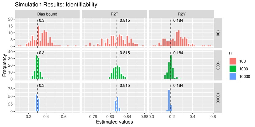
Figure 1: Histograms of estimated values of the width of the bias bound (first column), $R^{2}_{d^{\top}T\sim U}$ (second column), and $R^{2}_{a^{\top}Y\sim U|T}$ (third column). Each row corresponds to a distinct sample size, and in each panel the dashed black line indicates the true value.

5.2 Identification region with negative controls

We now highlight how negative controls can shift or reduce the size of the partial identification region, and how the extent of this depends greatly on specific choice of negative control. For illustrative purposes, we conduct experiments using one large simulated dataset of $n=10^{6}$ to minimize the estimation uncertainty stemming from sampling variability. We compare three identification regions: those without negative control adjustments, those computed using the analytical approach with negative controls, and those computed using the numerical approach with negative controls. For this comparison, we consider nine different scenarios, which are summarized in Table 1. The first seven scenarios correspond to the case with a single negative control contrast ($J=1$), where we assume that $Z_{1,1}=1$ and all other elements of $Z$ are zero. The last two scenarios correspond to the case with multiple negative control contrasts ($J=2$), where we assume that $Z_{1,1}=Z_{6,1}=1$ and all other elements of $Z$ are zero. Noting that the negative control identification regions are affected by the association between $a^{\top}\Gamma$ and $b^{\top}_{j}\Gamma$ as well as the association between $\Delta tB:=(t_{1}-t_{2})B$ and $\Delta t^{NC}B:=\left(t_{1}^{(j,1)}-t_{2}^{(j,1)}\right)B$, we explore different values of $a$ and different treatment contrasts $\Delta t=(t_{1}-t_{2})$ as described in Table 1. The three partial identification regions are presented along with the true bias values in Figure 3.

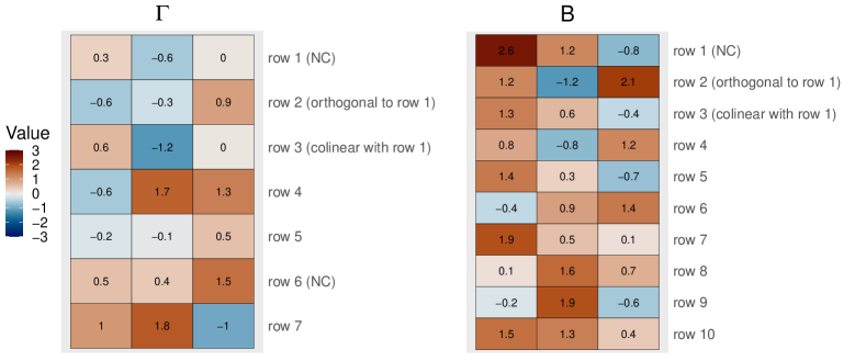
Figure 2: Heatmaps of $\Gamma$ and $B$. For the single negative control contrast case ($J=1$), the pair of the first outcome and first treatment is used as a negative control treatment-outcome pair. For the multiple negative control contrast case ($J=2$), the pair of the first outcome and first treatment and the pair of the sixth outcome and the first treatment are used as negative control treatment-outcome pairs.

Scenario	Estimand of interest		Negative controls		$a^{\top}\Gamma$ and $b_{j}^{\top}\Gamma$	$\Delta tB$ and $\Delta t^{NC}B$
	$a$	$\Delta t$	$b_{j}$	$\Delta t^{NC}$
Single negative control contrast ($J=1$):
(O, O)	$e_{2}^{q}$	$e_{2}^{k}$			orthogonal	orthogonal
(O, C)	$e_{2}^{q}$	$e_{3}^{k}$			orthogonal	colinear
(C, O)	$e_{3}^{q}$	$e_{2}^{k}$			colinear	orthogonal
(C, C)	$e_{3}^{q}$	$e_{3}^{k}$	$e_{1}^{q}$	$e_{1}^{k}$	colinear	colinear
(C, N)	$e_{3}^{q}$	$e_{4}^{k}$			colinear	neither
(N, C)	$e_{4}^{q}$	$e_{3}^{k}$			neither	colinear
(N, N)	$e_{4}^{q}$	$e_{5}^{k}$			neither	neither
Multiple negative control contrasts ($J=2$):
(ON, C)	$e_{2}^{q}$	$e_{3}^{k}$	$e_{1}^{q}$, $e_{6}^{q}$	$e_{1}^{k}$	orthogonal, neither	colinear
(NN, N)	$e_{4}^{q}$	$e_{5}^{k}$			neither, neither	neither

Table 1: The nine scenarios we considered in the estimation of our estimand of interest, $\text{PATE}_{a,t_{1},t_{2}}$. For the columns of $a$ and $b_{j}$, $e_{i}^{q}$ indicates a canonical basis vector of length $q$, implying that we focus on the $i$th outcome. For the columns of $\Delta t$ and $\Delta t^{NC}$, $e_{i}^{k}$ indicates a canonical basis vector of length $k$, implying that we focus on the $i$th treatment, where $\Delta t:=t_{1}-t_{2}=t_{1}$ with fixed $t_{2}=0_{k}$ and $\Delta t^{NC}:=t_{1}^{(j,1)}-t_{2}^{(j,1)}=t_{1}^{(j,1)}$ with fixed $t_{2}^{(j,1)}=0_{k}$.

In the first two scenarios, where $a^{\top}\Gamma$ and $b^{\top}_{j}\Gamma$ are orthogonal, the negative controls do not change the partial identification region, regardless of the association between $\Delta tB$ and $\Delta t^{NC}B$. This shows that when the confounding mechanisms for the outcome of interest and the negative control outcome are orthogonal, we obtain no benefit from negative controls. In scenarios three to five, the opposite is true as $a^{\top}\Gamma$ and $b^{\top}_{j}\Gamma$ are colinear, and we see both a bias correction and a reduction in the size of the partial identification region, though the nature of this depends on the confounding mechanism for the treatment and negative control treatment contrast. When the confounding mechanisms for the treatments are orthogonal, no benefit from the negative controls is seen, but when the treatment contrast and negative control treatment contrast have colinear confounding mechanisms, the treatment effect is point identified. In scenarios six through nine, including the cases with multiple negative controls, we observe varying magnitudes of bias correction and width reduction in the partial identification region after introducing negative controls and the nature of the partial identification regions depend on the choice of negative controls. Across all scenarios, the true value of bias is captured with and without negative controls. This underscores the potential of negative controls to reduce the size of the partial identification regions for treatment effects.

Another interesting observation is the relationship between the analytic negative control regions and the ones computed numerically. When looking at only one negative control contrast these two regions largely agree with each other. This is good for the analytic intervals, which have the potential to be conservative, but that is not seen here. Bigger differences are seen when looking at situations with multiple negative control contrasts. In the first of these scenarios, the numeric intervals are split into two separate intervals, rather than a single contiguous interval. This shows a large benefit of the numeric approach to the partial identification regions, as these split intervals can provide more information about the possible values of the causal effect than the analytic intervals, which are forced to be a single interval, and therefore contain a wider set of possible values. In scenario 8, the bias is actually identified up to its sign, but this is only reflected in the numeric interval, while the analytic interval shows no change relative to the interval without negative controls. The final scenario shows the conservativeness of the analytic intervals, as the numeric interval is much tighter as it can provide sharp bounds on the causal effect. Note that there are a couple of scenarios, such as scenarios 4 and 6, where the numeric intervals are slightly wider than the analytic ones. This is because our numeric approach to finding the partial identification region only finds approximate solutions, which tends to widen the intervals, though only by a small amount.

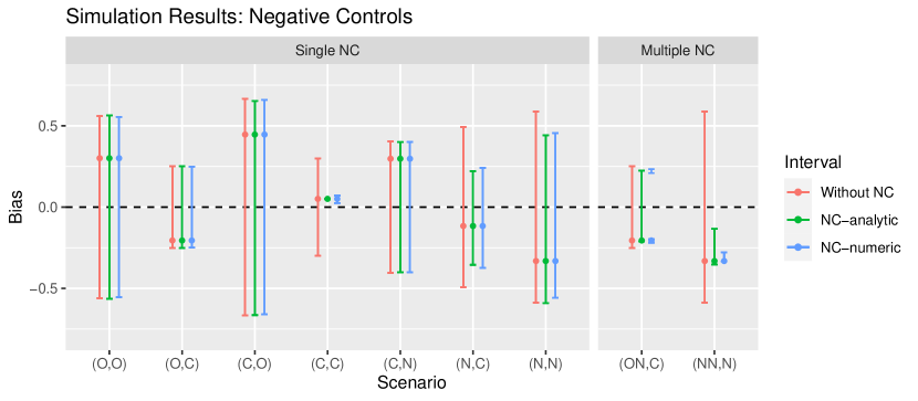
Figure 3: Estimated partial identification regions for the confounding bias when $n=10^{6}$: those computed without negative control adjustments (in red), those computed using our analytical approach with negative controls (in green), and those computed using our numerical approach with negative controls (in blue). The dot displayed alongside each interval indicates the true bias.

6 Discussion

In this paper, we proposed a sensitivity analysis framework that assesses the robustness of causal findings against omitted confounding bias in the presence of multiple treatments and outcomes. Under a factor confounding assumption, the strength of the association between the unmeasured confounders and both the treatment and outcome, expressed as partial $R^{2}$ values, is shown to be identifiable. This shows the advantage of simultaneously modeling multiple treatments and outcomes, as we are able to obtain partial identification regions for causal effects that are fully identifiable from the observed data as opposed to standard sensitivity analyses that incorporate sensitivity parameters that are not identifiable. Moreover, we show how additional information on negative control variables can reduce the size of the partial identification region. The incorporation of negative controls is particularly interesting in the multi-treatment and multi-outcome setting, as information from a separate negative control treatment-outcome pair can strengthen the causal conclusions about the estimand of interest. For the computation of the partial identification region under a negative control assumption, we proposed two novel approaches: a numerical approach using optimization over the Stiefel manifold, and an analytical approach that yields a closed-form solution for the partial identification region. Our theoretical and empirical studies suggest that the proposed framework can offer informative insights about causal effects even in the presence of unmeasured confounding variables.

There are a number of potentially interesting future research directions that could expand upon this work and make sensitivity analysis in multi-treatment and multi-outcome settings more widely applicable. For one, we have focused on continuous treatments here, which facilitates the use of the factor models used throughout, but extending these ideas to categorical treatments and generalized linear models would be an important extension of this work. Additionally, our current sensitivity analysis relies on the factor confounding assumption, and it would be useful to study the robustness of the sensitivity analysis procedure to violations of this assumption. Lastly, we studied the refinement of the partial identification region in the presence of negative controls, but other a priori assumptions, such as sparsity of treatment effects, could be incorporated as well. Extending our computational approach to these other situations would be natural extension that would broaden the scope of sensitivity analyses in this setting.

Appendix A Technical Details

A.1 Proof of Theorem 1

Proof.

The omitted confounding bias is bounded as follows:

$$\text{Bias}_{a,t_{1},t_{2}}^{2} =\left(a^{\top}\Gamma\Sigma_{u|t}^{-1/2}\mu_{u|\Delta t}\right)^{2}$$

$$=\|a^{\top}\Gamma\|_{2}^{2}\|\Sigma_{u|t}^{-1/2}\mu_{u|\Delta t}\|_{2}^{2}\cos^{2}(\theta_{a,t_{1},t_{2}})$$

$$\leq\|a^{\top}\Gamma\|_{2}^{2}\|\Sigma_{u|t}^{-1/2}\mu_{u|\Delta t}\|_{2}^{2},$$

where $\theta_{a,t_{1},t_{2}}$ represents the angle between the vectors $a^{\top}\Gamma$ and $\Sigma_{u|t}^{-1/2}\mu_{u|\Delta t}$. This completes the proof, and the bound can be reached when $a^{\top}\Gamma$ is colinear with $\Sigma_{u|t}^{-1/2}\mu_{u|\Delta t}$. ∎

A.2 Proof of identification results

Proof.

We first show the identification of $\|a^{\top}\Gamma\|_{2}$. Under the condition (C1) of Assumption 4, $\Gamma\Gamma^{\top}$ and $\Sigma_{y|t,u}$ is uniquely determined from

$$\text{Cov}[Y-g(T)|T=t] =\Gamma\Sigma_{u|t}^{-1/2}\text{Cov}(U|T=t)(\Gamma\Sigma_{u|t}^{-1/2})^{\top}+\text{Cov}(\epsilon_{Y})$$

$$=\Gamma\Sigma_{u|t}^{-1/2}\Sigma_{u|t}\Sigma_{u|t}^{-1/2}\Gamma^{\top}+\Sigma_{y|t,u}$$

$$=\Gamma\Gamma^{\top}+\Sigma_{y|t,u},$$

by applying Lemma 5.1 and Theorem 5.1 of Anderson & Rubin (1956) to the factor model (3), $\Gamma$ is identified up to rotations from the right under the factor confounding assumption. In other words, $\Gamma$ is identified up to multiplication on the right by an orthogonal matrix, and thus any admissible value for $\Gamma$ can be written as $\widetilde{\Gamma}=\Gamma R$ with an arbitrary $m\times m$ orthogonal matrix $R$ (Miao et al. 2022). Then, $\|a^{\top}\Gamma\|_{2}$, which is rotation-invariant, is identified as follows.

$$\|a^{\top}\widetilde{\Gamma}\|_{2}^{2} =\|a^{\top}\Gamma R\|_{2}^{2}$$

$$=a^{\top}\Gamma R(\Gamma R)^{\top}a$$

$$=a^{\top}\Gamma\Gamma^{\top}a$$

$$=\|a^{\top}\Gamma\|_{2}^{2},$$

since $RR^{\top}=I$.

Next, we show the identification of $\|\Sigma_{u|t}^{-1/2}\mu_{u|\Delta t}\|_{2}$, by applying the same idea to the factor model (2). Under condition (C2) of Assumption 4, $BB^{\top}$ and $\Sigma_{t|u}$ are uniquely determined from $\text{Cov}(T)=BB^{\top}+\text{Cov}(\epsilon_{t})=BB^{\top}+\Sigma_{t|u}$, and any admissible value for $B$ can be written as $\widetilde{B}=BR$ where $R$ is again an arbitrary $m\times m$ orthogonal matrix. Then, the conditional distribution of $U$ given $T$ with $\widetilde{B}$ is

$$f_{\widetilde{B}}(u|T=t)\sim N_{m}(\widetilde{\mu}_{u|t},\widetilde{\Sigma}_{u|t}),$$

with

$$\widetilde{\mu}_{u|t} =\widetilde{B}^{\top}(\widetilde{B}\widetilde{B}^{\top}+\Sigma_{t|u})^{-1}t$$

$$=R^{\top}B^{\top}(BB^{\top}+\Sigma_{t|u})^{-1}t$$

$$=R^{\top}\mu_{u|t},$$

$$\widetilde{\Sigma}_{u|t} =I_{m}-\widetilde{B}^{\top}(\widetilde{B}\widetilde{B}^{\top}+\Sigma_{t|u})^{-1}\widetilde{B}$$

$$=I_{m}-R^{\top}B^{\top}(BB^{\top}+\Sigma_{t|u})^{-1}BR$$

$$=R^{\top}\Sigma_{u|t}R,$$

where $\mu_{u|t}$ and $\Sigma_{u|t}$ are from (4). Then, we can show that

$$\|\widetilde{\Sigma}_{u|t}^{-1/2}\widetilde{\mu}_{u|\Delta t}\|^{2}_{2} =\|(R^{\top}\Sigma_{u|t}R)^{-1/2}(R^{\top}\mu_{u|\Delta t})\|^{2}_{2}$$

$$=\text{tr}\left\{(R^{\top}\mu_{u|\Delta t})^{\top}(R^{\top}\Sigma_{u|t}R)^{-1}(R^{\top}\mu_{u|\Delta t})\right\}$$

$$=\text{tr}\left(\mu_{u|\Delta t}^{\top}\Sigma_{u|t}^{-1}\mu_{u|\Delta t}\right)$$

$$=\|\Sigma_{u|t}^{-1/2}\mu_{u|\Delta t}\|^{2}_{2},$$

where $RR^{\top}=I$, which implies that $\|\Sigma_{u|t}^{-1/2}\mu_{u|\Delta t}\|_{2}$ is identified. Combining the identification results, the bias bound is identifiable under the conditions (C1) and (C2), which completes the proof. ∎

Remark. The identification of the two partial R-squared values in (10) immediately follows from the proof. Specifically, with any $R$ such that $RR^{\top}=I$, we have that

$$R^{2}_{a^{\top}Y\sim U|T} =\frac{\|a^{\top}\Gamma\|_{2}^{2}}{a^{\top}\Sigma_{y|t}a}=\frac{\|a^{\top}\Gamma R\|_{2}^{2}}{a^{\top}\Sigma_{y|t}a}=\frac{\|a^{\top}\widetilde{\Gamma}\|_{2}^{2}}{a^{\top}\Sigma_{y|t}a},$$

$$R^{2}_{d^{\top}T\sim U} =\frac{\|d^{\top}B\|_{2}^{2}}{d^{\top}\Sigma_{t}d}=\frac{\|d^{\top}BR\|_{2}^{2}}{d^{\top}\Sigma_{t}d}=\frac{\|d^{\top}\widetilde{B}\|_{2}^{2}}{d^{\top}\Sigma_{t}d}.$$

A.3 Algorithm for numerical approach in Section 3.4

We here outline the algorithm used to numerically determine the negative control partial identification regions. Note that we aim to minimize

$$\mathcal{F}(\widetilde{R})=(a^{\top}\widetilde{\Gamma}\widetilde{R}M_{1}-c_{1})^{2}+\sum_{j=1}^{J}\|b_{j}^{\top}\widetilde{\Gamma}\widetilde{R}M_{2,j}-c_{2,j}\|_{2}^{2},$$

with

$$\nabla_{\widetilde{R}}\mathcal{F}(\widetilde{R})=2(\widetilde{\Gamma}^{\top}aa^{\top}\widetilde{\Gamma}\widetilde{R}M_{1}M_{1}^{\top}-c_{1}\widetilde{\Gamma}^{\top}aM_{1})+2\sum_{j=1}^{J}(\widetilde{\Gamma}^{\top}b_{j}b_{j}^{\top}\widetilde{\Gamma}RM_{2,j}M_{2,j}^{\top}-\widetilde{\Gamma}^{\top}b_{j}c_{2,j}M_{2,j}^{\top}),$$

where $\widetilde{R}\in\mathcal{V}_{m,m}$, the Stiefel manifold of all $m\times m$ orthogonal matrices. In order to run the algorithm, we first need to (i) specify $t_{1}$, $t_{2}$, and $a$ for the estimand of interest, and $\boldsymbol{b}=(b_{1},\cdots,b_{J})$ for the negative control contrasts, (ii) obtain $\widehat{\Gamma}$, $\widehat{\Sigma}_{u|t}$, $\widehat{\mu}_{u|\Delta t}$, $\check{g}(\cdot)$, $M_{u|\Delta t,j}$, and $b_{j}^{\top}\check{\mathcal{G}}_{j}$ for $j=1,\cdots,J$ using the estimation method described in Section 4, (iii) define $\Theta=\{\theta_{a,t_{1},t_{2}}:-1\leq\cos(\theta_{a,t_{1},t_{2}})\leq 1\}$, a set of all candidate values of $\theta_{a,t_{1},t_{2}}$, and (iv) specify a threshold value, $\delta$, as a selection criterion for $\theta_{a,t_{1},t_{2}}$. Note that under the notation introduced in Section 3.4, $\delta=\delta_{1}=\delta_{2}/J$. Then the algorithm can be summarized in Algorithm 1. The idea is to find $\theta_{a,t_{1},t_{2}}$ values that align with the conditions mentioned in Section 3.4. Once Algorithm 1 is implemented, we obtain $\Theta_{NC}$ and then construct the negative control partial identification region for bias as follows:

$$\text{Bias}_{a,t_{1},t_{2}}\in\left\{\|a^{\top}\Gamma\|_{2}\|\Sigma_{u|t}^{-1/2}\mu_{u|\Delta t}\|_{2}\cos(\theta_{a,t_{1},t_{2}}):\theta_{a,t_{1},t_{2}}\in\Theta_{NC}\right\}.$$

Input: $t_{1}$, $t_{2}$, $a$ (estimand of interest), $\widehat{\Gamma}$, $\widehat{\Sigma}_{u|t}$, $\widehat{\mu}_{u|\Delta t}$ (estimates), $\boldsymbol{b}$, $M_{u|\Delta t,j}$, $b_{j}^{\top}\check{\mathcal{G}}_{j}$, $j=1,\cdots,J$ (negative controls), $\Theta$ (a set of candidate values of $\theta_{a,t_{1},t_{2}}$), $\delta$ (threshold value).

Output: $\Theta_{NC}$, a set of all selected values of $\theta_{a,t_{1},t_{2}}$.

Compute $M_{1}\leftarrow\widehat{\Sigma}_{u|t}^{-1/2}\widehat{\mu}_{u|\Delta t}$.

Compute $M_{2,j}\leftarrow M_{u|\Delta t,j}$ and $c_{2,j}\leftarrow b_{j}^{\top}\check{\mathcal{G}}_{j}$ for $j=1,\cdots,J$.

Initialize $\widetilde{R}_{0}$, by generating a random orthogonal matrix from the uniform distribution on the Stiefel manifold using the rustiefel function of the rstiefel package.

Initialize $\Theta_{NC}\leftarrow\varnothing$ (an empty set).

for each $\theta_{a,t_{1},t_{2}}\in\Theta$ do

      

      Compute $c_{1}\leftarrow\|a^{\top}\widehat{\Gamma}\|_{2}\|\widehat{\Sigma}_{u|t}^{-1/2}\widehat{\mu}_{u|\Delta t}\|_{2}\cos(\theta_{a,t_{1},t_{2}})$.

      

      Update $\widetilde{R}^{*}\leftarrow\arg\min_{\widetilde{R}\in\mathcal{V}_{m,m}}\mathcal{F}(\widetilde{R})$ using the optStiefel function of the rstiefel package, with $\widetilde{R}_{0}$ as the initial value and $\widetilde{\Gamma}\leftarrow\widehat{\Gamma}$.

       if $(a^{\top}\widetilde{\Gamma}\widetilde{R}^{*}M_{1}-c_{1})^{2}\leq\delta$ and $\frac{1}{J}\sum_{j=1}^{J}\|b_{j}^{\top}\widetilde{\Gamma}\widetilde{R}^{*}M_{2,j}-c_{2,j}\|_{2}^{2}\leq\delta$ then

            Add $\theta_{a,t_{1},t_{2}}$ to the set $\Theta_{NC}$.

       end if

      Set $\widetilde{R}_{0}\leftarrow\widetilde{R}^{*}$.

end for

Algorithm 1 Algorithm for finding negative control partial identification region

A.4 Proof of Theorem 2

Proof.

We assume that we only have a single negative control contrast. This provides us information about the plausible values of $b_{j}^{\top}\Gamma$. To ensure that the negative control assumptions are compatible, the solution for (12) exists as

$$b_{j}^{\top}\Gamma=b_{j}^{\top}\check{\mathcal{G}}_{j}M_{u|\Delta t,j}^{\dagger}+w_{b,j}(I-M_{u|\Delta t,j}M_{u|\Delta t,j}^{\dagger}),$$ (26)

for some arbitrary $m$-dimensional row vector $w_{b,j}$, if and only if

$$b_{j}^{\top}\check{\mathcal{G}}_{j}M_{u|\Delta t,j}^{\dagger}M_{u|\Delta t,j}=b_{j}^{\top}\check{\mathcal{G}}_{j}$$

holds (Penrose 1955), where $M_{u|\Delta t,j}^{\dagger}$ denotes a generalized inverse of $M_{u|\Delta t,j}$, $M_{u|\Delta t,j}M_{u|\Delta t,j}^{\dagger}$ is the projection matrix onto the column space of $M_{u|\Delta t,j}$, and $M_{u|\Delta t,j}^{\dagger}M_{u|\Delta t,j}$ is the projection matrix onto the row space of $M_{u|\Delta t,j}$. Note here that if $c_{j}=m$, we have that $M_{u|\Delta t,j}^{\dagger}$ is a standard inverse instead of a generalized inverse, and we are able to identify $b_{j}^{\top}\Gamma$.

We also have a different piece of information about the relationship between $a^{\top}\Gamma$ and $b_{j}^{\top}\Gamma$, which we have from our factor model assumptions. This is given by

$$b_{j}^{\top}\Gamma\Gamma^{\top}a=a^{\top}\Gamma\Gamma^{\top}b_{j}=k_{ab}$$ (27)

for some constant $k_{ab}$ that is identified from our factor model assumptions. We can combine these two pieces of information to see that

$$a^{\top}\Gamma =k_{ab}({D}^{\top})^{\dagger}+w_{a}\{I-({D}^{\top})({D}^{\top})^{\dagger}\},$$ (28)

where

$$D:=b_{j}^{\top}\Gamma=b_{j}^{\top}\check{\mathcal{G}}_{j}M_{u|\Delta t,j}^{\dagger}+w_{b,j}(I-M_{u|\Delta t,j}M_{u|\Delta t,j}^{\dagger})$$

is an $m$-dimensional row vector. Since $D$ is a vector, we here use the fact that

$$D^{\dagger}=\frac{D^{\top}}{\|D\|_{2}^{2}}=\frac{D^{\top}}{\|b_{j}^{\top}\Gamma\|_{2}^{2}}=\frac{D^{\top}}{k_{bb}}~{}~{}~{}\text{and thus}~{}~{}~{}(D^{\dagger})^{\top}=(D^{\top})^{\dagger}=\frac{D}{k_{bb}},$$

where $k_{bb}:=b_{j}^{\top}\Gamma\Gamma^{\top}b_{j}$ is an identifiable constant.

Combining these ideas together, for treatment contrast $\Delta t=t_{1}-t_{2}$, we can see that the omitted variable bias of $\text{PATE}_{a,t_{1},t_{2}}$ is

$$\text{Bias}_{a,t_{1},t_{2}} =a^{\top}\Gamma\Sigma_{u|t}^{-1/2}\mu_{u|\Delta t}$$

$$=k_{ab}({D}^{\top})^{\dagger}\Sigma_{u|t}^{-1/2}\mu_{u|\Delta t}+w_{a}\{I-({D}^{\top})({D}^{\top})^{\dagger}\}\Sigma_{u|t}^{-1/2}\mu_{u|\Delta t}$$

$$=\frac{k_{ab}}{k_{bb}}b_{j}^{\top}\Gamma\Sigma_{u|t}^{-1/2}\mu_{u|\Delta t}+w_{a}\{I-({D}^{\top})({D}^{\top})^{\dagger}\}\Sigma_{u|t}^{-1/2}\mu_{u|\Delta t}$$

$$=\underbrace{\frac{k_{ab}}{k_{bb}}b_{j}^{\top}\check{\mathcal{G}}_{j}M_{u|\Delta t,j}^{\dagger}\Sigma_{u|t}^{-1/2}\mu_{u|\Delta t}}_{(I)\text{ bias correction}}+\underbrace{\frac{k_{ab}}{k_{bb}}w_{b,j}(I-M_{u|\Delta t,j}M_{u|\Delta t,j}^{\dagger})\Sigma_{u|t}^{-1/2}\mu_{u|\Delta t}}_{(II)}$$

$$~{}~{}~{}+\underbrace{w_{a}\{I-({D}^{\top})({D}^{\top})^{\dagger}\}\Sigma_{u|t}^{-1/2}\mu_{u|\Delta t}}_{(III)}$$

The first term (I) is identifiable and is the bias correction term for the center of our new interval. Now all that is left to do is to bound $(II)$ and $(III)$, which include the free vectors $w_{a}$ and $w_{b,j}$ and are therefore unidentifiable.

We can first bound $(II)$. We can see that the $l_{2}$ norm of this vector is given by

$$~{}~{}~{}\left\|\frac{k_{ab}}{k_{bb}}w_{b,j}(I-M_{u|\Delta t,j}M_{u|\Delta t,j}^{\dagger})\Sigma_{u|t}^{-1/2}\mu_{u|\Delta t}\right\|_{2}^{2}$$

$$=\left\|\frac{k_{ab}}{k_{bb}}w_{b,j}(I-M_{u|\Delta t,j}M_{u|\Delta t,j}^{\dagger})^{2}\Sigma_{u|t}^{-1/2}\mu_{u|\Delta t}\right\|_{2}^{2}$$

$$\leq\left\|\frac{k_{ab}}{k_{bb}}w_{b,j}(I-M_{u|\Delta t,j}M_{u|\Delta t,j}^{\dagger})\right\|_{2}^{2}\left\|(I-M_{u|\Delta t,j}M_{u|\Delta t,j}^{\dagger})\Sigma_{u|t}^{-1/2}\mu_{u|\Delta t}\right\|_{2}^{2},$$

where the first equality holds because $(I-M_{u|\Delta t,j}M_{u|\Delta t,j}^{\dagger})$ is an idempotent matrix. Taking the $l_{2}$ norm of both sides of (26) and re-arranging terms gives us that

$$\|w_{b,j}(I-M_{u|\Delta t,j}M_{u|\Delta t,j}^{\dagger})\|_{2}^{2}=\|b_{j}^{\top}\Gamma\|_{2}^{2}-\|b_{j}^{\top}\check{\mathcal{G}}_{j}M_{u|\Delta t,j}^{\dagger}\|_{2}^{2}.$$

Hence,

$$|(II)| \leq\left\|\frac{k_{ab}}{k_{bb}}w_{b,j}(I-M_{u|\Delta t,j}M_{u|\Delta t,j}^{\dagger})\right\|_{2}\left\|(I-M_{u|\Delta t,j}M_{u|\Delta t,j}^{\dagger})\Sigma_{u|t}^{-1/2}\mu_{u|\Delta t}\right\|_{2}$$

$$=\Big{|}\frac{k_{ab}}{k_{bb}}\Big{|}\sqrt{k_{bb}-\|b_{j}^{\top}\check{\mathcal{G}}_{j}M_{u|\Delta t,j}^{\dagger}\|_{2}^{2}}\left\|(I-M_{u|\Delta t,j}M_{u|\Delta t,j}^{\dagger})\Sigma_{u|t}^{-1/2}\mu_{u|\Delta t}\right\|_{2},$$

where we use the notation $k_{bb}=\|b_{j}^{\top}\Gamma\|_{2}^{2}$.

In a similar way, we can get an upper bound of $(III)$. We here use the fact that

$$~{}~{}~{}\|w_{a}\{I-({D}^{\top})({D}^{\top})^{\dagger}\}\Sigma_{u|t}^{-1/2}\mu_{u|\Delta t}\|_{2}^{2}$$

$$=\|w_{a}\{I-({D}^{\top})({D}^{\top})^{\dagger}\}^{2}\Sigma_{u|t}^{-1/2}\mu_{u|\Delta t}\|_{2}^{2}$$

$$\leq\|w_{a}\{I-({D}^{\top})({D}^{\top})^{\dagger}\}\|_{2}^{2}\|\{I-({D}^{\top})({D}^{\top})^{\dagger}\}\Sigma_{u|t}^{-1/2}\mu_{u|\Delta t}\|_{2}^{2}$$

and, from (28),

$$\|w_{a}\{I-({D}^{\top})({D}^{\top})^{\dagger}\}\|_{2}^{2} =\|a^{\top}\Gamma\|_{2}^{2}-\|k_{ab}({D}^{\top})^{\dagger}\|_{2}^{2}$$

$$=k_{aa}-\|k_{ab}({D}^{\top})^{\dagger}\|_{2}^{2},$$

where $k_{aa}:=\|a^{\top}\Gamma\|_{2}^{2}$. To simplify this further, we use that

$$\|({D}^{\top})^{\dagger}\|_{2}^{2}=\left\|\frac{D}{k_{bb}}\right\|_{2}^{2}=\frac{1}{k_{bb}^{2}}\|D\|_{2}^{2}=\frac{k_{bb}}{k_{bb}^{2}}=\frac{1}{k_{bb}}.$$

Combining all of this gives us our final bound on $(III)$, which is given by

$$|(III)| \leq\|w_{a}\{I-({D}^{\top})({D}^{\top})^{\dagger}\}\|_{2}\|\{I-({D}^{\top})({D}^{\top})^{\dagger}\}\Sigma_{u|t}^{-1/2}\mu_{u|\Delta t}\|_{2}$$

$$\leq\sqrt{k_{aa}-\frac{k_{ab}^{2}}{k_{bb}}}\|\{I-({D}^{\top})({D}^{\top})^{\dagger}\}\Sigma_{u|t}^{-1/2}\mu_{u|\Delta t}\|_{2}$$

$$\leq\sqrt{k_{aa}-\frac{k_{ab}^{2}}{k_{bb}}}\|\Sigma_{u|t}^{-1/2}\mu_{u|\Delta t}\|_{2}.$$

The final step is done because the $\|\{I-({D}^{\top})({D}^{\top})^{\dagger}\}\Sigma_{u|t}^{-1/2}\mu_{u|\Delta t}\|_{2}$ term is unidentifiable, which means that different rotations of either the $\Gamma$ or $B$ matrices can lead to different values of this quantity. Putting all of these thoughts together gives us the following interval for the confounding bias of $a^{\top}Y$ in the presence of the negative controls:

$$\frac{k_{ab}}{k_{bb}}b_{j}^{\top}\check{\mathcal{G}}_{j}M_{u|\Delta t,j}^{\dagger}\Sigma_{u|t}^{-1/2}\mu_{u|\Delta t}\quad\pm$$

$$\Bigg{(}\Big{|}\frac{k_{ab}}{k_{bb}}\Big{|}\sqrt{k_{bb}-\|b_{j}^{\top}\check{\mathcal{G}}_{j}M_{u|\Delta t,j}^{\dagger}\|_{2}^{2}}\|(I-M_{u|\Delta t,j}M_{u|\Delta t,j}^{\dagger})\Sigma_{u|t}^{-1/2}\mu_{u|\Delta t}\|_{2}$$

$$+\sqrt{k_{aa}-\frac{k_{ab}^{2}}{k_{bb}}}\ \|\Sigma_{u|t}^{-1/2}\mu_{u|\Delta t}\|_{2}\Bigg{)}.$$

Note that, we obtain point identification of the treatment effect if (i) we have $m$ negative control contrasts ($c_{j}=m$), and (ii) either our negative control outcome is the same as the outcome of interest ($a=b_{j}$) or $a^{\top}\Gamma$ is colinear with $b_{j}^{\top}\Gamma$. ∎

A.5 Proof of Theorem 3

Proof.

Suppose that there are $J$ outcomes with at least one negative control treatment. Letting $\mathcal{Q}\subset\{1,\cdots,q\}$ denote a set of the indices of such outcomes and $\text{card}(\cdot)$ denote the cardinality of a set, we have that $J=\text{card}(\mathcal{Q})$. The negative control contrast provides us information about the plausible values of $b_{j}^{\top}\Gamma$ for $j\in\mathcal{Q}$. In particular, we can see the following. By Theorem 2 of Penrose (1955), a necessary and sufficient condition for (12) to have a solution is

$$b_{j}^{\top}\check{\mathcal{G}}_{j}M_{u|\Delta t,j}^{\dagger}M_{u|\Delta t,j}=b_{j}^{\top}\check{\mathcal{G}}_{j},$$

in which case the general solution exists as

$$b_{j}^{\top}\Gamma=b_{j}^{\top}\check{\mathcal{G}}_{j}M_{u|\Delta t,j}^{\dagger}+w_{b,j}(I-M_{u|\Delta t,j}M_{u|\Delta t,j}^{\dagger})$$ (29)

for some arbitrary $m$-dimensional row vector $w_{b,j}$, where $M_{u|\Delta t,j}^{\dagger}$ denotes a generalized inverse of $M_{u|\Delta t,j}$, $M_{u|\Delta t,j}M_{u|\Delta t,j}^{\dagger}$ is the projection matrix onto the column space of $M_{u|\Delta t,j}$, and $M_{u|\Delta t,j}^{\dagger}M_{u|\Delta t,j}$ is the projection matrix onto the row space of $M_{u|\Delta t,j}$. Notice that (29) satisfies

$$\|w_{b,j}(I-M_{u|\Delta t,j}M_{u|\Delta t,j}^{\dagger})\|^{2}_{2}=\|b_{j}^{\top}\Gamma\|^{2}_{2}-\|b_{j}^{\top}\check{\mathcal{G}}_{j}M_{u|\Delta t,j}^{\dagger}\|^{2}_{2}.$$ (30)

For notational convenience, we denote the decomposition of (29) by $b_{j}^{\top}\Gamma:=D_{j}=D_{j}^{(1)}+D_{j}^{(2)}$ where $D_{j}^{(1)}:=b_{j}^{\top}\check{\mathcal{G}}_{j}M_{u|\Delta t,j}^{\dagger}$ and $D_{j}^{(2)}:=w_{b,j}(I-M_{u|\Delta t,j}M_{u|\Delta t,j}^{\dagger})$. It will also be useful later to break this matrix into two components since $D^{(1)}$ contains the estimable components and $D^{(2)}$ refers to the unidentified portion. We refer to the stacked version of $D_{j}$’s as $\boldsymbol{D}=[D_{1}^{\top},\dots,D_{J}^{\top}]^{\top}$, which is a $J\times m$ matrix. We can also define $\boldsymbol{b}=[b_{1},b_{2},\dots,b_{J}]$, which is a $q\times J$ matrix that has each individual $b_{j}$ as its columns. In other words, in the matrix form, we have that

$$\left(\begin{array}[]{c}b_{1}^{\top}\Gamma\\ \vdots\\ b_{J}^{\top}\Gamma\\ \end{array}\right)=\left(\begin{array}[]{c}b_{1}^{\top}\check{\mathcal{G}}_{1}M_{u|\Delta t,1}^{\dagger}+w_{b,1}(I-M_{u|\Delta t,1}M_{u|\Delta t,1}^{\dagger})\\ \vdots\\ b_{J}^{\top}\check{\mathcal{G}}_{J}M_{u|\Delta t,J}^{\dagger}+w_{b,J}(I-M_{u|\Delta t,J}M_{u|\Delta t,J}^{\dagger})\\ \end{array}\right)=\left(\begin{array}[]{c}D_{1}^{(1)}+D_{1}^{(2)}\\ \vdots\\ D_{J}^{(1)}+D_{J}^{(2)}\\ \end{array}\right)=\left(\begin{array}[]{c}D_{1}\\ \vdots\\ D_{J}\\ \end{array}\right),$$

i.e., $\boldsymbol{b}^{\top}\Gamma=\boldsymbol{D}^{(1)}+\boldsymbol{D}^{(2)}=\boldsymbol{D}$.

Under our factor modeling assumptions, we are able to identify

$$a^{\top}\Gamma\Gamma^{\top}\boldsymbol{b}:=K_{ab}$$ (31)

where $K_{ab}$ is a $J$-dimensional row vector. Using the fact that $\boldsymbol{b}^{\top}\Gamma=\boldsymbol{D}$, we know that $a^{\top}\Gamma\boldsymbol{D}^{\top}:=K_{ab}$, and thus all solutions to $a^{\top}\Gamma$ can be written as

$$a^{\top}\Gamma=K_{ab}(\boldsymbol{D}^{\top})^{\dagger}+w_{a}\left\{I-(\boldsymbol{D}^{\top})(\boldsymbol{D}^{\top})^{\dagger}\right\}$$ (32)

for some arbitrary $m$-dimensional row vector $w_{a}$. This follows

$$\left\|w_{a}\left\{I-(\boldsymbol{D}^{\top})(\boldsymbol{D}^{\top})^{\dagger}\right\}\right\|^{2}_{2}=\|a^{\top}\Gamma\|^{2}_{2}-\|K_{ab}(\boldsymbol{D}^{\top})^{\dagger}\|^{2}_{2}.$$ (33)

Given that the rank of $\boldsymbol{D}$ is $J$, we can re-write $\boldsymbol{D}^{\dagger}$ as

$$\boldsymbol{D}^{\dagger}=\boldsymbol{D}^{\top}(\boldsymbol{D}\boldsymbol{D}^{\top})^{-1}$$

and $(\boldsymbol{D}^{\top})^{\dagger}=(\boldsymbol{D}^{\dagger})^{\top}=(\boldsymbol{D}\boldsymbol{D}^{\top})^{-1}\boldsymbol{D}$, which implies that

$$a^{\top}\Gamma =K_{ab}(\boldsymbol{D}\boldsymbol{D}^{\top})^{-1}\boldsymbol{D}+w_{a}\left\{I-(\boldsymbol{D}^{\top})(\boldsymbol{D}^{\top})^{\dagger}\right\}$$

$$=K_{ab}(\boldsymbol{D}\boldsymbol{D}^{\top})^{-1}\boldsymbol{D}^{(1)}+K_{ab}(\boldsymbol{D}\boldsymbol{D}^{\top})^{-1}\boldsymbol{D}^{(2)}+w_{a}\left\{I-(\boldsymbol{D}^{\top})(\boldsymbol{D}^{\top})^{\dagger}\right\}.$$

The bias for the estimand of interest is given by

$$~{}~{}~{}a^{\top}\Gamma\Sigma_{u|t}^{-1/2}\mu_{u|\Delta t}$$

$$=K_{ab}(\boldsymbol{D}\boldsymbol{D}^{\top})^{-1}\boldsymbol{D}^{(1)}\Sigma_{u|t}^{-1/2}\mu_{u|\Delta t}+K_{ab}(\boldsymbol{D}\boldsymbol{D}^{\top})^{-1}\boldsymbol{D}^{(2)}\Sigma_{u|t}^{-1/2}\mu_{u|\Delta t}+w_{a}\left\{I-(\boldsymbol{D}^{\top})(\boldsymbol{D}^{\top})^{\dagger}\right\}\Sigma_{u|t}^{-1/2}\mu_{u|\Delta t}$$

$$=\underbrace{K_{ab}K_{bb}^{-1}\boldsymbol{D}^{(1)}\Sigma_{u|t}^{-1/2}\mu_{u|\Delta t}}_{(I)\text{ bias correction}}+\underbrace{K_{ab}(\boldsymbol{D}\boldsymbol{D}^{\top})^{-1}\boldsymbol{D}^{(2)}\Sigma_{u|t}^{-1/2}\mu_{u|\Delta t}}_{(II)}+\underbrace{w_{a}\left\{I-(\boldsymbol{D}^{\top})(\boldsymbol{D}^{\top})^{\dagger}\right\}\Sigma_{u|t}^{-1/2}\mu_{u|\Delta t}}_{(III)},$$

where $K_{bb}:=\boldsymbol{D}\boldsymbol{D}^{\top}$, and thus the first term $(I)$ is identifiable as our bias correction. The remaining two terms, $(II)$ and $(III)$, are not identifiable and therefore we will bound them to create regions for the confounding bias that are compatible with the negative control conditions. Before bounding these terms, it is helpful to write $(II)$ as

$$(II)=\sum_{j=1}^{J}\alpha_{j}w_{b,j}(I-M_{u|\Delta t,j}M_{u|\Delta t,j}^{\dagger})\Sigma_{u|t}^{-1/2}\mu_{u|\Delta t},$$

where $\alpha_{j}$ is the $j$th element of the $J$-dimensional row vector $K_{ab}(\boldsymbol{D}\boldsymbol{D}^{\top})^{-1}=K_{ab}K_{bb}^{-1}$. We know that, for $j=1,\cdots,J$,

$$~{}~{}~{}\left\{\alpha_{j}w_{b,j}(I-M_{u|\Delta t,j}M_{u|\Delta t,j}^{\dagger})\Sigma_{u|t}^{-1/2}\mu_{u|\Delta t}\right\}^{2}$$

$$=\left\{\alpha_{j}w_{b,j}(I-M_{u|\Delta t,j}M_{u|\Delta t,j}^{\dagger})^{2}\Sigma_{u|t}^{-1/2}\mu_{u|\Delta t}\right\}^{2}$$

$$=\|\alpha_{j}w_{b,j}(I-M_{u|\Delta t,j}M_{u|\Delta t,j}^{\dagger})^{2}\Sigma_{u|t}^{-1/2}\mu_{u|\Delta t}\|^{2}_{2}$$

$$\leq\alpha_{j}^{2}\|w_{b,j}(I-M_{u|\Delta t,j}M_{u|\Delta t,j}^{\dagger})\|^{2}_{2}\|(I-M_{u|\Delta t,j}M_{u|\Delta t,j}^{\dagger})\Sigma_{u|t}^{-1/2}\mu_{u|\Delta t}\|^{2}_{2}.$$

The first equality holds because $(I-M_{u|\Delta t,j}M_{u|\Delta t,j}^{\dagger})$ is an idempotent matrix. Combining this with (30),

$$|(II)| \leq\sum_{j=1}^{J}|\alpha_{j}|\|w_{b,j}(I-M_{u|\Delta t,j}M_{u|\Delta t,j}^{\dagger})\|_{2}\|(I-M_{u|\Delta t,j}M_{u|\Delta t,j}^{\dagger})\Sigma_{u|t}^{-1/2}\mu_{u|\Delta t}\|_{2}$$

$$=\sum_{j=1}^{J}|\alpha_{j}|\sqrt{\|b_{j}^{\top}\Gamma\|^{2}_{2}-\|b_{j}^{\top}\check{\mathcal{G}}_{j}M_{u|\Delta t,j}^{\dagger}\|^{2}_{2}}\|(I-M_{u|\Delta t,j}M_{u|\Delta t,j}^{\dagger})\Sigma_{u|t}^{-1/2}\mu_{u|\Delta t}\|_{2},$$

where $\|b_{j}^{\top}\Gamma\|^{2}_{2}=(K_{bb})_{j,j}$ is the $(j,j)$th entry of $K_{bb}$, which is identifiable.

Now we need to provide a bound for the final term $(III)$ in the expression for the bias of interest. In a similar way, this can be done with (33) as,

$$|(III)| \leq\left\|w_{a}\left\{I-(\boldsymbol{D}^{\top})(\boldsymbol{D}^{\top})^{\dagger}\right\}\right\|_{2}\left\|\left\{I-(\boldsymbol{D}^{\top})(\boldsymbol{D}^{\top})^{\dagger}\right\}\Sigma_{u|t}^{-1/2}\mu_{u|\Delta t}\right\|_{2}$$

$$=\sqrt{K_{aa}-\|K_{ab}K_{bb}^{-1}\boldsymbol{b}^{\top}\Gamma\|^{2}_{2}}\left\|\left\{I-(\boldsymbol{D}^{\top})(\boldsymbol{D}^{\top})^{\dagger}\right\}\Sigma_{u|t}^{-1/2}\mu_{u|\Delta t}\right\|_{2}$$

$$\leq\sqrt{K_{aa}-\|K_{ab}K_{bb}^{-1}\boldsymbol{b}^{\top}\Gamma\|^{2}_{2}}\|\Sigma_{u|t}^{-1/2}\mu_{u|\Delta t}\|_{2},$$

where $K_{aa}:=a^{\top}\Gamma\Gamma^{\top}a$ is identifiable and $K_{ab}(\boldsymbol{D}^{\top})^{\dagger}=K_{ab}K_{bb}^{-1}\boldsymbol{b}^{\top}\Gamma$. Putting all of this together, we can see that the confounding bias is in the region given by

$$K_{ab}K_{bb}^{-1}\boldsymbol{D}^{(1)}\Sigma_{u|t}^{-1/2}\mu_{u|\Delta t}\quad\pm$$

$$\Bigg{(}\sum_{j=1}^{J}|\alpha_{j}|\sqrt{\|b_{j}^{\top}\Gamma\|^{2}_{2}-\|b_{j}^{\top}\check{\mathcal{G}}_{j}M_{u|\Delta t,j}^{\dagger}\|^{2}_{2}}\|(I-M_{u|\Delta t,j}M_{u|\Delta t,j}^{\dagger})\Sigma_{u|t}^{-1/2}\mu_{u|\Delta t}\|_{2}$$

$$+\sqrt{K_{aa}-\|K_{ab}K_{bb}^{-1}\boldsymbol{b}^{\top}\Gamma\|^{2}_{2}}\|\Sigma_{u|t}^{-1/2}\mu_{u|\Delta t}\|_{2}\Bigg{)},$$

which is equivalent to

$$K^{*}\boldsymbol{D}^{*}\Sigma_{u|t}^{-1/2}\mu_{u|\Delta t}\quad\pm$$

$$\Bigg{(}\sum_{j=1}^{J}|(K^{*})_{j}|\sqrt{(K_{bb})_{j,j}-\|(\boldsymbol{D}^{*})_{j\cdot}\|^{2}_{2}}\|(I-M_{u|\Delta t,j}M_{u|\Delta t,j}^{\dagger})\Sigma_{u|t}^{-1/2}\mu_{u|\Delta t}\|_{2}$$

$$+\sqrt{K_{aa}-\|K^{*}\boldsymbol{b}^{\top}\Gamma\|^{2}_{2}}\|\Sigma_{u|t}^{-1/2}\mu_{u|\Delta t}\|_{2}\Bigg{)},$$

where $K^{*}:=K_{ab}K_{bb}^{-1}$ and $\boldsymbol{D}^{*}:=\boldsymbol{D}^{(1)}$. ∎

Appendix B Additional Results

B.1 Determination of number of factors for factor analysis

One key component of factor analysis is determining how many factors to retain, as it is generally unknown in real applications. The methods for the determination include: vss.comp1 and vss.comp2 (very simple structure criterion with complexity 1 and 2; (Revelle & Rocklin 1979)), map (minimum average partial criterion Velicer (1976)), BIC (BIC for each number of factors), adjBIC (sample size adjusted BIC for each number of factors), parallel.fa and parallel.pc (number of factors/components with eigenvalues greater than those of random data; parallel analysis Horn (1965)), and eigen (number of eigenvalues greater than 1).

We apply these eight methods to the models (2) and (3) to estimate the number of unmeasured confounders. We adopt the same settings as in Section 5, but take subsets of the $\Gamma$ and $B$ matrices by excluding their last columns, assuming the true value of $m$ is 2. Figure 4 shows that $m$ is typically estimated at its true value in this simulation setting, while the very simple structure criterion tends to over-estimate $m$, and the minimum average partial criterion often under-estimates it for model (3).

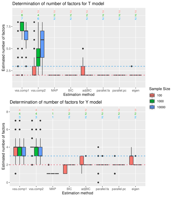
Figure 4: Boxplots of the number of factors determined by eight different methods. The numbers displayed alongside the boxplots represent the median value of $m$ determined over 300 simulation replicates. The red dashed line indicates the true value of $m$, and the blue dashed line indicates the maximum value of $m$ that satisfies the factor confounding assumption.

The value of $m$ determined by the aforementioned methods does not necessarily satisfy our factor model assumption. In real applications with data consisting of a known number of outcomes and treatments, we can first determine the maximum value of $m$ that meets our factor confounding assumption. Then we can see whether any given value of $m$ in a factor model (ranging from 1 to its maximum value) is sufficient to capture the full dimensionality of the given data. The factanal function in R provides such a significant test. In our simulation setting, where the true value of $m$ is 2 and the maximum value of $m$ is 3 given that $k=10$ and $q=7$, we found that $m$ is correctly determined at its true value most of the time and is very rarely under-estimated.

B.2 Results with incorrect number of unmeasured confounders

For practical applications, it is worth studying the sensitivity of our findings to misspecification of the number of unmeasured confounders. Figure 5 illustrates how the bias bound and the two partial $R^{2}$ values are estimated if $m$ were to be under or over-estimated. These values are identifiable when $m$ is correctly specified. The figure shows that the bias bound and the two partial $R^{2}$ values tend to be under-estimated when $m$ is under-estimated, and conversely, they tend to be over-estimated when $m$ is over-estimated. This implies that over-estimating $m$ results in a conservative bias bound and a conservative partial identification region.

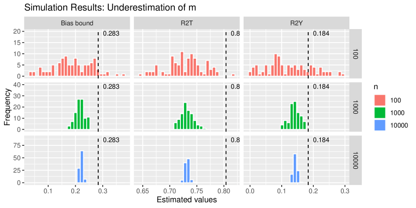
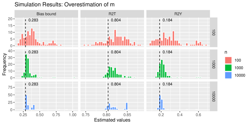
Figure 5: Histograms of estimated values of bias bound (first column), $R^{2}_{b^{\top}T\sim U}$ (second column), $R^{2}_{a^{\top}Y\sim U|T}$ (third column) when $m$ is under-estimated as 1 or over-estimated as 3. In each panel, the dashed black line indicates the true value.

References

- (1)
- Anderson & Rubin (1956) Anderson, T. & Rubin, H. (1956), Statistical inference in, in ‘Proceedings of the Third Berkeley Symposium on Mathematical Statistics and Probability: Held at the Statistical Laboratory, University of California, December, 1954, July and August, 1955’, Vol. 1, Univ of California Press, p. 111.
- Burnett et al. (2018) Burnett, R., Chen, H., Szyszkowicz, M., Fann, N., Hubbell, B., Pope III, C. A., Apte, J. S., Brauer, M., Cohen, A., Weichenthal, S. et al. (2018), ‘Global estimates of mortality associated with long-term exposure to outdoor fine particulate matter’, Proceedings of the National Academy of Sciences 115(38), 9592–9597.
- Carone et al. (2020) Carone, M., Dominici, F. & Sheppard, L. (2020), ‘In pursuit of evidence in air pollution epidemiology: the role of causally driven data science’, Epidemiology (Cambridge, Mass.) 31(1), 1.
- Chernozhukov et al. (2022) Chernozhukov, V., Cinelli, C., Newey, W., Sharma, A. & Syrgkanis, V. (2022), Long story short: Omitted variable bias in causal machine learning, Technical report, National Bureau of Economic Research.
- Cinelli & Hazlett (2020) Cinelli, C. & Hazlett, C. (2020), ‘Making sense of sensitivity: Extending omitted variable bias’, Journal of the Royal Statistical Society Series B-Statistical Methodology 82(1), 39–67.
- Cohen et al. (2017) Cohen, A. J., Brauer, M., Burnett, R., Anderson, H. R., Frostad, J., Estep, K., Balakrishnan, K., Brunekreef, B., Dandona, L., Dandona, R. et al. (2017), ‘Estimates and 25-year trends of the global burden of disease attributable to ambient air pollution: an analysis of data from the global burden of diseases study 2015’, The lancet 389(10082), 1907–1918.
- Cornfield et al. (1959) Cornfield, J., Haenszel, W., Hammond, E. C., Lilienfeld, A. M., Shimkin, M. B. & Wynder, E. L. (1959), ‘Smoking and lung cancer: recent evidence and a discussion of some questions’, Journal of the National Cancer institute 22(1), 173–203.
- Ding & VanderWeele (2016a) Ding, P. & VanderWeele, T. J. (2016a), ‘Sensitivity analysis without assumptions’, Epidemiology (Cambridge, Mass.) 27(3), 368.
- Ding & Vanderweele (2016b) Ding, P. & Vanderweele, T. J. (2016b), ‘Sharp sensitivity bounds for mediation under unmeasured mediator-outcome confounding’, Biometrika 103(2), 483–490.
- Dockery et al. (1993) Dockery, D. W., Pope, C. A., Xu, X., Spengler, J. D., Ware, J. H., Fay, M. E., Ferris Jr, B. G. & Speizer, F. E. (1993), ‘An association between air pollution and mortality in six us cities’, New England journal of medicine 329(24), 1753–1759.
- Dominici & Zigler (2017) Dominici, F. & Zigler, C. (2017), ‘Best practices for gauging evidence of causality in air pollution epidemiology’, American journal of epidemiology 186(12), 1303–1309.
- Freidling & Zhao (2022) Freidling, T. & Zhao, Q. (2022), ‘Sensitivity analysis with the -calculus’, arXiv preprint arXiv:2301.00040 .
- Friedman (1991) Friedman, J. H. (1991), ‘Multivariate adaptive regression splines’, The annals of statistics 19(1), 1–67.
- Hoff & Franks (2019) Hoff, P. & Franks, A. (2019), rstiefel: Random Orthonormal Matrix Generation and Optimization on the Stiefel Manifold. R package version 1.0.0.
- Horn (1965) Horn, J. L. (1965), ‘A rationale and test for the number of factors in factor analysis’, Psychometrika 30, 179–185.
- Hu et al. (2023) Hu, J. K., Zorzetto, D. & Dominici, F. (2023), ‘A bayesian nonparametric method to adjust for unmeasured confounding with negative controls’, arXiv preprint arXiv:2309.02631 .
- Huang et al. (2015) Huang, C., Nichols, C., Liu, Y., Zhang, Y., Liu, X., Gao, S., Li, Z. & Ren, A. (2015), ‘Ambient air pollution and adverse birth outcomes: a natural experiment study’, Population health metrics 13, 1–7.
- Imai et al. (2010) Imai, K., Keele, L. & Yamamoto, T. (2010), ‘Identification, inference and sensitivity analysis for causal mediation effects’.
- Imbens (2003) Imbens, G. W. (2003), ‘Sensitivity to exogeneity assumptions in program evaluation’, American Economic Review 93(2), 126–132.
- Kong et al. (2022) Kong, D., Yang, S. & Wang, L. (2022), ‘Identifiability of causal effects with multiple causes and a binary outcome’, Biometrika 109(1), 265–272.
- Luechinger (2014) Luechinger, S. (2014), ‘Air pollution and infant mortality: A natural experiment from power plant desulfurization’, Journal of health economics 37, 219–231.
- Manisalidis et al. (2020) Manisalidis, I., Stavropoulou, E., Stavropoulos, A. & Bezirtzoglou, E. (2020), ‘Environmental and health impacts of air pollution: a review’, Frontiers in public health 8, 14.
- Manski (1990) Manski, C. F. (1990), ‘Nonparametric bounds on treatment effects’, The American Economic Review 80(2), 319–323.
- McCandless et al. (2007) McCandless, L. C., Gustafson, P. & Levy, A. (2007), ‘Bayesian sensitivity analysis for unmeasured confounding in observational studies’, Statistics in medicine 26(11), 2331–2347.
- Miao et al. (2022) Miao, W., Hu, W., Ogburn, E. L. & Zhou, X.-H. (2022), ‘Identifying effects of multiple treatments in the presence of unmeasured confounding’, Journal of the American Statistical Association pp. 1–15.
- Miao et al. (2018) Miao, W., Shi, X. & Tchetgen, E. T. (2018), ‘A confounding bridge approach for double negative control inference on causal effects’, arXiv preprint arXiv:1808.04945 .
- Penrose (1955) Penrose, R. (1955), A generalized inverse for matrices, in ‘Mathematical proceedings of the Cambridge philosophical society’, Vol. 51, Cambridge University Press, pp. 406–413.
- Pope Iii et al. (2002) Pope Iii, C. A., Burnett, R. T., Thun, M. J., Calle, E. E., Krewski, D., Ito, K. & Thurston, G. D. (2002), ‘Lung cancer, cardiopulmonary mortality, and long-term exposure to fine particulate air pollution’, Jama 287(9), 1132–1141.
- Portney (1990) Portney, P. R. (1990), ‘Policy watch: economics and the clean air act’, Journal of Economic Perspectives 4(4), 173–181.
- Revelle & Rocklin (1979) Revelle, W. & Rocklin, T. (1979), ‘Very simple structure: An alternative procedure for estimating the optimal number of interpretable factors’, Multivariate behavioral research 14(4), 403–414.
- Rich (2017) Rich, D. Q. (2017), ‘Accountability studies of air pollution and health effects: lessons learned and recommendations for future natural experiment opportunities’, Environment international 100, 62–78.
- Rosenbaum (1987) Rosenbaum, P. R. (1987), ‘Sensitivity analysis for certain permutation inferences in matched observational studies’, Biometrika 74(1), 13–26.
- Rosenbaum (1988) Rosenbaum, P. R. (1988), ‘Sensitivity analysis for matching with multiple controls’, Biometrika 75(3), 577–581.
- Rosenbaum (1991) Rosenbaum, P. R. (1991), ‘Sensitivity analysis for matched case-control studies’, Biometrics pp. 87–100.
- Rosenbaum (2002a) Rosenbaum, P. R. (2002a), ‘Covariance adjustment in randomized experiments and observational studies’, Statistical Science 17(3), 286–327.
- Rosenbaum (2002b) Rosenbaum, P. R. (2002b), Overt bias in observational studies, Springer.
- Rosenbaum & Rubin (1983) Rosenbaum, P. R. & Rubin, D. B. (1983), ‘Assessing sensitivity to an unobserved binary covariate in an observational study with binary outcome’, Journal of the Royal Statistical Society: Series B (Methodological) 45(2), 212–218.
- Rubin (1974) Rubin, D. B. (1974), ‘Estimating causal effects of treatments in randomized and nonrandomized studies.’, Journal of Educational Psychology 66(5), 688.
- Schwartz et al. (2023) Schwartz, J., Wei, Y., Dominici, F. & Yazdi, M. D. (2023), ‘Effects of low-level air pollution exposures on hospital admission for myocardial infarction using multiple causal models’, Environmental Research p. 116203.
- Shi et al. (2020) Shi, X., Miao, W. & Tchetgen, E. T. (2020), ‘A selective review of negative control methods in epidemiology’, Current epidemiology reports 7, 190–202.
- Small (2007) Small, D. S. (2007), ‘Sensitivity analysis for instrumental variables regression with overidentifying restrictions’, Journal of the American Statistical Association 102(479), 1049–1058.
- Sommer et al. (2021) Sommer, A. J., Leray, E., Lee, Y. & Bind, M.-A. C. (2021), ‘Assessing environmental epidemiology questions in practice with a causal inference pipeline: An investigation of the air pollution-multiple sclerosis relapses relationship’, Statistics in Medicine 40(6), 1321–1335.
- Splawa-Neyman et al. (1990) Splawa-Neyman, J., Dabrowska, D. M. & Speed, T. P. (1990), ‘On the application of probability theory to agricultural experiments. essay on principles. section 9.’, Statistical Science pp. 465–472.
- VanderWeele (2010) VanderWeele, T. J. (2010), ‘Bias formulas for sensitivity analysis for direct and indirect effects’, Epidemiology (Cambridge, Mass.) 21(4), 540.
- VanderWeele & Ding (2017) VanderWeele, T. J. & Ding, P. (2017), ‘Sensitivity analysis in observational research: introducing the e-value’, Annals of internal medicine 167(4), 268–274.
- Veitch & Zaveri (2020) Veitch, V. & Zaveri, A. (2020), ‘Sense and sensitivity analysis: Simple post-hoc analysis of bias due to unobserved confounding’, Advances in Neural Information Processing Systems 33, 10999–11009.
- Velicer (1976) Velicer, W. F. (1976), ‘Determining the number of components from the matrix of partial correlations’, Psychometrika 41, 321–327.
- Zhang & Ding (2022) Zhang, M. & Ding, P. (2022), ‘Interpretable sensitivity analysis for the baron-kenny approach to mediation with unmeasured confounding’, arXiv preprint arXiv:2205.08030 .
- Zheng et al. (2021) Zheng, J., D’Amour, A. & Franks, A. (2021), ‘Copula-based sensitivity analysis for multi-treatment causal inference with unobserved confounding’, arXiv preprint arXiv:2102.09412 .
- Zheng et al. (2022) Zheng, J., D’Amour, A. & Franks, A. (2022), Bayesian inference and partial identification in multi-treatment causal inference with unobserved confounding, in ‘International Conference on Artificial Intelligence and Statistics’, PMLR, pp. 3608–3626.
- Zheng et al. (2023) Zheng, J., Wu, J., D’Amour, A. & Franks, A. (2023), ‘Sensitivity to unobserved confounding in studies with factor-structured outcomes’, Journal of the American Statistical Association (just-accepted), 1–23.