Efficient Reinforcement Learning from Partial Observability

Abstract

In most real-world reinforcement learning applications, state information is only partially observable, which breaks the Markov decision process assumption and leads to inferior performance for algorithms that conflate observations with state. Partially Observable Markov Decision Processes (POMDPs), on the other hand, provide a general framework that allows for partial observability to be accounted for in learning, exploration and planning, but presents significant computational and statistical challenges. To address these difficulties, we develop a representation-based perspective that leads to a coherent framework and tractable algorithmic approach for practical reinforcement learning from partial observations. We provide a theoretical analysis for justifying the statistical efficiency of the proposed algorithm, and also empirically demonstrate the proposed algorithm can surpass state-of-the-art performance with partial observations across various benchmarks, advancing reliable reinforcement learning towards more practical applications.

1 Introduction

Reinforcement learning (RL) addresses the problem of making sequential decisions that maximize a cumulative reward through interaction and observation in an environment (Mnih et al., 2013; Levine et al., 2016). The Markov decision process (MDP) has been the standard mathematical model used for most RL algorithm design. However, the success of MDP-based RL algorithms (Zhang et al., 2022; Ren et al., 2023c) relies on an assumption that state information is fully observable, which implies that the optimal policy is memoryless, i.e., optimal actions can be selected based purely on the current state (Puterman, 2014). However, such an assumption typically does not hold in practice. For example, in chatbot learning (Jiang et al., 2021) or video game control (Mnih et al., 2013) only dialogue exchanges or images are observed, from which state information only can be partially inferred. The violation of full observability can lead to significant performance degeneration of MDP-based RL algorithms in such scenarios.

The Partially Observed Markov Decision Process (POMDP) (Åström, 1965) has been proposed to extend the classical MDP formulation by introducing observation variables that only give partial information about the underlying latent state (Hauskrecht and Fraser, 2000; Roy and Gordon, 2002; Chen et al., 2016). This extension greatly expands the practical applicability of POMDPs over MDPs, but the additional uncertainty over the underlying state given only observations creates a non-Markovian dependence between successive observations, even though Markovian dependence is preserved between latent states. Consequently, the optimal policy for a POMDP is no longer memoryless but entire-history dependent, expanding the state complexity exponentially w.r.t. horizon length. Such a non-Markovian dependence creates significant computational and statistical challenges in planning, and in learning and exploration. In fact, without additional assumptions, computing an optimal policy for a POMDP with known dynamics (i.e., planning) is PSPACE-complete (Papadimitriou and Tsitsiklis, 1987), while the sample complexity of learning for POMDPs grows exponentially w.r.t. the horizon (Jin et al., 2020a).

Despite the worst case hardness of POMDPs, given their importance in practice, there has been extensive work on developing practical RL algorithms that can cope with partial observations. One common heuristic is to extend MDP-based RL algorithms by maintaining a history window over observations to encode a policy or value function, e.g., recurrent neural networks (Wierstra et al., 2007; Hausknecht and Stone, 2015; Zhu et al., 2017). Such algorithms have been applied to many real-world applications with image- or text-based observations (Berner et al., 2019; Jiang et al., 2021), sometimes even surpassing human-level performance (Mnih et al., 2013; Kaufmann et al., 2023).

These empirical successes have motivated investigation into structured POMDPs that allow some of the core computational and statistical complexities to be overcome, and provides an improved understanding of exploitable structure and practical new algorithms with rigorous justification. For example, the concept of decodability has been used to express POMDPs where the latent state can be exactly recovered from a window of past observations (Efroni et al., 2022; Guo et al., 2023). Observability is another special structure, where the $m$-step emission model is assumed to be full-rank, allowing the latent state to be identified from $m$ future observation sequences (Jin et al., 2020a; Golowich et al., 2022; Liu et al., 2022, 2023). Such structures eliminate unbounded history dependence, and thus, reduce the computational and statistical complexity. However, most works rely on the existence of an ideal computational oracle for planning, which, unsurprisingly, is infeasible in most cases, hence difficult to apply in practice. Although there have been a few attempts to overcome the computational complexity of POMDPS, these algorithms are either only applicable to the tabular setting (Golowich et al., 2022) or rely on an integration oracle that quickly become intractable for large observation spaces (Guo et al., 2018). This gap immediately motivates the question:

• Can efficient and practical RL algorithms be designed for partial observations by exploiting natural structures?

By “efficient" we mean the statistical complexity avoids an exponential dependence on history length, while by “practical" we mean that every component of learning, planning and exploration can be easily implemented and applied in practical settings. In this paper, we provide an affirmative answer to this question. More specifically,

• We reveal for the first time that an $L$-decodable POMDP admits a sufficient representation, the Multi-step Latent Variable Representation ($\mu$LV-Rep), that supports exact and tractable linear representation of the value functions (Section 4.1), breaking the fundamental computational barriers explained in more detail in Section 3.

• We design a computationally efficient planning algorithm that can implement both the principles of optimism and pessimism in the face of uncertainty for online and offline POMDPs respectively, by leveraging the learned sufficient representation $\mu$LV-Rep (Section 4.2).

• We provide a theoretical analysis of the sample complexity of the proposed algorithm, justifying its efficiency in balancing exploitation versus exploration in Section 5.

• We conduct a comprehensive empirical comparison to current existing RL algorithms for POMDPs on several benchmarks, demonstrating the superior empirical performance of $\mu$LV-Rep (Section 7).

2 Preliminaries

We follow the definition of a POMDP given in (Efroni et al., 2022; Liu et al., 2022, 2023), which is formally denoted as a tuple $\mathcal{P}=(\mathcal{S},\mathcal{A},\mathcal{O},r,H,\rho_{0},\mathbb{P},\mathbb{O})$, where $\mathcal{S}$ is the state space, $\mathcal{A}$ is the action space, and $\mathcal{O}$ is the observation space. The positive integer $H$ denotes the horizon length, $\rho_{0}$ is the initial state distribution, $r:\mathcal{O}\times\mathcal{A}\to[0,1]$ is the reward function, $\mathbb{P}(\cdot|s,a):\mathcal{S}\times\mathcal{A}\to\Delta(\mathcal{S})$ is the transition kernel capturing dynamics over latent states, and $\mathbb{O}(\cdot|s):\mathcal{S}\to\Delta(\mathcal{O})$ is the emission kernel, which induces an observation from a given state.

Initially, the agent starts at a state $s_{0}$ drawn from $\rho_{0}(s)$. At each step $h$, the agent selects an action $a$ from $\mathcal{A}$. This leads to the generation of a new state $s_{h+1}$ following the distribution $\mathbb{P}(\cdot|s_{h},a_{h})$, from which the agent observes $o_{h+1}$ according to $\mathbb{O}(\cdot|s_{h+1})$. The agent also receives a reward $r(o_{h+1},a_{h+1})$. Observing $o$ instead of the true state $s$ leads to a non-Markovian transition between observations, which means we need to consider policies $\pi_{h}:\mathcal{O}\times(\mathcal{A}\times\mathcal{O})^{h}\to\Delta(\mathcal{A})$ that depend on the entire history, denoted by $\tau_{h}=\{o_{0},a_{0},\cdots,o_{h}\}$. Let $[H]:=\left\{0,\ldots,H\right\}$. Then the value associated with policy $\pi=\{\pi_{h}\}_{h\in[H]}$ is defined as $v^{\pi}=\mathbb{E}_{\pi}\left[\sum_{h\in[H]}r(o_{h},a_{h})\right]$. The goal is to find the optimal policy $\pi^{*}=\arg\max_{\pi}v^{\pi}$. Note that the MDP given by $\mathcal{M}=(\mathcal{S},\mathcal{A},r,H,\rho_{0},\mathbb{P})$ is a special case of a POMDP, where the state space $\mathcal{S}$ is equivalent to the observation space $\mathcal{O}$, and the emission kernel $\mathbb{O}(o|s)$ is defined as $\delta(o=s)$.

Define the belief function $b(\cdot):\mathcal{O}\times(\mathcal{A}\times\mathcal{O})^{h}\to\Delta(\mathcal{S})$. Let $b(s_{1}|o_{1})=\mathbb{P}(s_{1}|o_{1})$. Then we can recursively compute:

$$b(s_{h+1}|\tau_{h+1})\!\propto\!\!\int_{\mathcal{S}}b(s_{h}|\tau_{h})\mathbb{P}(s_{h+1}|s_{h},a_{h})\mathbb{O}(o_{h+1}|s_{h+1})ds_{h}.$$ (1)

With such a definition, one can convert a POMDP to an equivalent MDP over beliefs, denoted as $\mathcal{M}_{b}=\left(\mathcal{B},\mathcal{A},R_{h},H,\mu_{b},T_{b}\right)$, where $\mathcal{B}\subseteq\Delta(\mathcal{S})$ represents the set of possible beliefs, $\mu_{b}(\cdot)=\int b(\cdot|o_{1})\mu(o_{1})do_{1}$, and

$$\mathbb{P}_{b}\left(b_{h+1}|b_{h},a_{h}\right)=\int\mathbf{1}_{b_{h+1}=b(\tau_{h},a_{h},o_{h+1})}\mathbb{P}(o_{h+1}|b_{h},a_{h})do_{h+1}.$$ (2)

Notice that $b(\cdot)\in\mathcal{B}$ is a mapping $b:\mathcal{O}\times(\mathcal{A}\times\mathcal{O})^{h}\to\Delta(\mathcal{S})$, i.e., each belief corresponds to a density measure over the state space, thus $\mathbb{P}_{b}\left(\cdot|b_{h},a_{h}\right)$ represents a conditional operator that characterizes the transition between belief distributions. For a given policy $\pi:\mathcal{B}\to\Delta(\mathcal{A})$, we can define the state value function $V_{h}^{\pi}(b_{h})$ and state-action value function $Q_{h}^{\pi}(b_{h},a_{h})$ respectively for the belief MDP (i.e., equivalently for the original POMDP) as:

$$V_{h}^{\pi}(b_{h})=\mathbb{E}\left[\sum_{t=h}^{H}r(o_{t},a_{t})|b_{h}\right],\quad$$

$$Q_{h}^{\pi}(b_{h},a_{h})=\mathbb{E}\left[\sum_{t=h}^{H}r(o_{t},a_{t})|b_{h},a_{h}\right].$$ (3)

Therefore, the Bellman equation can be expressed as

$$V_{h}^{\pi}(b_{h})=\mathbb{E}_{\pi}\left[Q_{h}^{\pi}(b_{h},a_{h})\right],\quad$$

$$Q_{h}^{\pi}(b_{h},a_{h})=r(o_{h},a_{h})+\mathbb{E}_{\mathbb{P}_{b}}\left[V_{h+1}^{\pi}(b_{h+1})\right].$$ (4)

Although this reformulation of a POMDP provides a reduction to an equivalent MDP, it is crucial to recognize that the equivalent MDP is based on beliefs, which are also not directly observed. More importantly, these beliefs are densities that depend on the entire history, hence the joint distribution is supported on a space of growing dimension, leading to exponential representation complexity even when the number of states is finite. These difficulties result in infeasible computational and statistical complexity (Papadimitriou and Tsitsiklis, 1987; Jin et al., 2020a), and reveal the inherent suboptimality of directly applying MDP-based RL algorithms in a POMDP. Moreover, incorporating function approximation in learning and planning is significantly more involved in a POMDP than an MDP.

Consequently, several special structures have been investigated in the theoretical literature to reduce the statistical complexity of learning in a POMDP. Specifically, $L$-decodability and $\gamma$-observability have been introduced in (Du et al., 2019; Efroni et al., 2022) and  (Golowich et al., 2022; Even-Dar et al., 2007) respectively.

Definition 1 ($L$-decodability (Efroni et al., 2022))

$\forall h\in[H]$, define

$$x_{h}\in\mathcal{X}:=(\mathcal{O}\times\mathcal{A})^{L-1}\times\mathcal{O},$$

$$x_{h}=(o_{h-L+1},a_{h-L+1},\cdots,o_{h}).$$ (5)

A POMDP is $L$-decodable if there exists a decoder $p^{*}:\mathcal{X}\to\Delta(\mathcal{S})$ such that $p^{*}(x_{h})=b(\tau_{h})$.

Definition 2 ($\gamma$-observability (Golowich et al., 2022; Even-Dar et al., 2007))

Denote $\left\langle\mathbb{O},b\right\rangle:=\int\mathbb{O}_{h}\left(\cdot|s\right)b\left(s\right)ds$, for arbitrary beliefs $b$ and $b^{\prime}$ over states. A POMDP is $\gamma$-observable if $\left\|\left\langle\mathbb{O},b\right\rangle-\left\langle\mathbb{O},b^{\prime}\right\rangle\right\|_{1}\geqslant\gamma\left\|b-b^{\prime}\right\|_{1}$.

Note that we slightly generalize the decodability definition of Efroni et al. (2022), which assumes $b(\tau_{h})$ is a Dirac measure on $\mathcal{S}$. It is worth noticing that $\gamma$-observability and $L$-decodability are highly related. Existing works have shown that a $\gamma$-observable POMDP can be well approximated by a decodable POMDP with a history of suitable length $L$ (Golowich et al., 2022; Uehara et al., 2022; Guo et al., 2023) (see Appendix B for a detailed discussion). Hence, in the main text, we focus on $L$-decodable POMDPs, which can be directly extended to $\gamma$-observable POMDPs.

Although these structural assumptions have been introduced to ensure the sample complexity of learning in a structured POMDP is reduced, the computational tractability of planning and exploring given such structures remains open.

3 Difficulties in Learning with POMDPs

Before attempting to design practical RL algorithms for structured POMDPs, we first demonstrate the generic difficulties of learning in POMDPs, including the difficulty of planning even in a known POMDP. These challenges only become more difficult when combined with the need to explore in an unknown POMDP during learning.

The major difficulty of planning in a known POMDP lies in evaluating the value function (Ross et al., 2008), which is necessary for both temporal-difference and policy gradient based planning and learning methods. For clarity in explaining the difficulties, consider estimating $Q^{\pi}$ for a given policy $\pi$. (The same difficulties arise in estimating $Q^{*}$.) Based on the Bellman equation (2), we have:

$$Q^{\pi}_{h}\left(b_{h},a_{h}\right)=r\left(o_{h},a_{h}\right)+\mathbb{E}_{\mathbb{P}(o_{h+1}|b_{h},a_{h})}\left[{V^{\pi}_{h+1}\left(b_{h+1}\right)}\right].$$

To execute dynamic programming in the $h^{\textrm{th}}$ time step, i.e., to determine $Q^{\pi}_{h}$, we require several components:

• The belief $b_{h+1}(\cdot)$ must be calculated, as defined in (1), which requires marginalization and renormalization, with a computational complexity proportional to the number of states. For continuous control, the calculation involves integration, which is intractable in general.

• Representing the value function $V_{h+1}^{\pi}(\cdot)$ quickly becomes intractable, even for discrete state and action spaces. In general, expressing $V_{h+1}^{\pi}(\cdot)$ requires space proportional to size of the support of beliefs, which is exponential w.r.t. the horizon. (The optimal value function $V_{h+1}^{*}\left(\cdot\right)$ can be represented by convex piece-wise linear function (Smallwood and Sondik, 1973), but the number of components can grow exponentially in the horizon.) For continuous state POMDPS, no compact characterization is yet known for the space of value functions.

• The expectation $\mathbb{E}_{\mathbb{P}(o_{h+1}|b_{h},a_{h})}\left[V^{\pi}\left(b_{h+1}\right)\right]$ requires integration w.r.t. the distribution $\mathbb{P}(o_{h+1}|b_{h},a_{h})=\int\mathbb{O}(o_{h+1}|s_{h+1})\mathbb{P}\left(s_{h+1}|s_{h},a_{h}\right)b_{h}\left(s_{h}\right)ds_{h}ds_{h+1}$ with computational cost proportional to the size of the support of beliefs, which is also exponential in the horizon.

These calculations are generally intractable in a POMDP, particularly one with a continuous state space. Due to this intractability, the exact calculation of the value function via the Bellman equation is generally infeasible. Consequently, many approximation methods have been proposed for each component of planning (Ross et al., 2008). However, the approximation error in each step can be amplified when these steps are composed through the Bellman recursion, leading to significantly suboptimal performance.

Due to promising theoretical results that exploit $\gamma$-observability or $L$-decodability to reduce the exponential dependence on horizon in terms of statistical complexity, there have been many attempts to exploit these properties to also achieve computationally tractable planning for RL in a POMDP. Golowich et al. (2022) construct an approximate MDP for an $L$-observable POMDP, whose approximation error can be characterized for planning. However, the proposed algorithm only works for POMDPs with discrete observations, states and actions. Alternatively, Guo et al. (2023) exploits low-rank latent dynamics in an $L$-decodable POMDP, which induces a nonlinear representation for value functions. Unfortunately, this nonlinear structure has not been shown to support any practical algorithm. To implement the backup step in dynamic programming for $Q^{\pi}$, the algorithm in (Guo et al., 2023) requires an integration-oracle to handle the nonlinearity, which is generally infeasible.

Another barrier to practical learning in a POMDP is exploration, which is usually implemented in planning by appealing to the principle of optimism in the face of uncertainty (OFU). Unfortunately, OFU usually requires not only the estimation of the model or value function, but also their uncertainty, e.g., a confidence interval in frequentist approaches (Liu et al., 2022, 2023) or the posterior in Bayesian approaches (Simchowitz et al., 2021). Practical and general implementations are not yet known in either case.

These major issues, which have not been carefully considered in empirical RL algorithms that leverage history-based neural networks (Wierstra et al., 2007; Hausknecht and Stone, 2015; Zhu et al., 2017), interact in ways that exaggerate the difficulty of developing efficient and practical RL algorithms for POMDPs.

4 Multi-step Latent Variable Representation

In this section, we develop the first computationally efficient planning and exploration algorithm by further leveraging the structure of an $L$-decodable POMDP. The main contribution is to identify a latent variable representation that can linearly represent the value function of an arbitrary policy in an $L$-step decodable POMDP. From this representational perspective, we show that explicit belief calculation can be bypassed and the backup step can be directly calculated via optimization. We then show how a latent variable representation learning algorithm can be designed, based upon (Ren et al., 2023b), that leads to the proposed Multi-step Latent Variable Representation ($\mu$LV-Rep) method.

4.1 Efficient Policy Evaluation from Key Observations

Although the equivalent belief MDP provides a Markovian Bellman recursion (2), as discussed in Section 3, this belief viewpoint hampers tractability in planning. In the following, we introduce the key observations that allow us to resolve the aforementioned difficulties in planning step-by-step.

Belief Elimination.

Our first key observation is that $L$-decodability eliminates an aspect of exponential complexity:

• In an $L$-decodable POMDP, it is sufficient to recover the belief state by an $L$-step memory $x_{h}$ rather than the entire history $\tau_{h}$.

This is exactly the definition of $L$-decodability given in Definition 1. From this observation that beliefs $b_{h}\left(s\right)$ can be represented with a decoder from $L$-step windows $x_{h}$ (1), we obtain the simplification $Q_{h}^{\pi}\left(b_{h}\left(\tau_{h}\right),a_{h}\right)=Q_{h}^{\pi}\left(b_{h}\left(x_{h}\right),a_{h}\right)$. In addition, $L$-decodability also helps reduce dependence in the dynamics, leading to $\mathbb{P}\left(o_{h+1}|b_{h}\left(\tau_{h}\right),a_{h}\right)=\mathbb{P}\left(o_{h+1}|b_{h}\left(x_{h}\right),a_{h}\right)$. This outcome reduces the statistical complexity, as previously exploited in (Efroni et al., 2022; Guo et al., 2023). However, it is not sufficient to ensure computationally friendly planning.

Next we make a second key observation that allows us to eliminate the explicit use of beliefs in the Bellman equation:

• An observation-based value function and transition model bypasses the necessity for belief computation.

That is, since $b_{h}\left(\cdot\right)$ is a mapping from the history $x_{h}$ to the space of probability densities over state, we can reparametrize the composition $Q_{h}^{\pi}\left(b_{h}(x_{h}),a_{h}\right)$ as $Q_{h}^{\pi}\left(x_{h},a_{h}\right)$, which is a function directly over $\left(x_{h},a_{h}\right)$. Similarly, we can also consider the transition dynamics directly defined over the observation history, $\mathbb{P}\left(o_{h+1}|x_{h},a_{h}\right)$, rather than work with the far more complex dynamics between successive beliefs. With such a reformulation, we avoid explicit dependence on beliefs in the $Q^{\pi}$-function and dynamics in the Bellman recursion (2). This resolves the first difficulty that arises from explicit belief calculation, leading to the simplified Bellman equation:

$$Q_{h}^{\pi}\left(x_{h},a_{h}\right)=r\left(o_{h},a_{h}\right)+\mathbb{E}_{\mathbb{P}^{\pi}\left(o_{h+1}|x_{h},a_{h}\right)}\left[V_{h+1}^{\pi}\left(x_{h+1}\right)\right].$$ (6)

Linear Representation for $Q^{\pi}$.

Next, we address a second key difficulty that arises in representing $V_{h+1}^{\pi}(x_{h+1})=\mathbb{E}_{a\sim\pi}\left[Q_{h+1}^{\pi}\left(x_{h+1},a_{h+1}\right)\right]$. We seek an exact representation that can be recursively maintained. Inspired by the success of representing value functions exactly in linear MDPs (Jin et al., 2020b; Yang and Wang, 2020), it is natural to consider $x_{h}$ as a mega-state (Efroni et al., 2022) and factorize the observation distribution in (6) as $\mathbb{P}\left(o_{h+1}|b_{h},a_{h}\right)=\left\langle\phi\left(x_{h},a_{h}\right),\mu\left(o_{h+1}\right)\right\rangle$ over basis functions $\phi$ and $\mu$. However, it is important to realize there is an additional dependence of $V_{h+1}^{\pi}(x_{h+1})$ on $(x_{h},a_{h})$, since

$$x_{h+1}=({\color[rgb]{1,0,0}o_{h-L+2},a_{h-L+2},\cdots,o_{h},a_{h},}o_{h+1})$$

has an overlap with

$$(x_{h},a_{h})=(o_{h-L+1},a_{h-L+1},{\color[rgb]{1,0,0}o_{h-L+2},a_{h-L+2},\cdots,o_{h},a_{h}}).$$

This overlap breaks the maintained linear structure, since

$$Q_{h}^{\pi}\left(b_{h},a_{h}\right)=r_{h}\left(o_{h},a_{h}\right)+\textstyle\left\langle\phi\left(x_{h},a_{h}\right),\underbrace{\int\mu\left(o_{h+1}\right)V_{h+1}\left(x_{h},a_{h},o_{h+1}\right)d{o_{h+1}}}_{w\left(x_{h},a_{h}\right)}\right\rangle.$$

That is, the nonlinearity in $w\left(x_{h},a_{h}\right)$ prevents the direct extension of linear MDPs with mega-states (Efroni et al., 2022) to the POMDP case (Guo et al., 2023).

Nevertheless, a linear representation for the value function can still be recovered if the dependence of the $h+1$-step value function on $(x_{h},a_{h})$ can be eliminated. The next key observation shows how this overlap might be avoided:

• By $L$-step decodability, $V_{h+L}^{\pi}(x_{h+L})$ is independent of $\left(x_{h},a_{h}\right)$.

This observation inspires us to consider the $L$-step Bellman equation for $Q_{h}^{\pi}\left(\tau_{h},a_{h}\right)$, which can be easily derived by expanding (2) forward in time to:

$$Q_{h}^{\pi}\left(x_{h},a_{h}\right)=\textstyle\mathbb{E}^{\pi}_{x_{h+1:h+L}|x_{h},a_{h}}\left[\sum_{i=h}^{h+L-1}r(o_{i},a_{i})+V_{h+L}^{\pi}(x_{h+L})\right].$$ (7)

At first glance, the $L$-step forward expansion only involves $V_{h+L}^{\pi}(x_{h+L})$, which would seem to eliminate the overlapping dependence of $x_{h+L}$ on $(x_{h},a_{h})$ due to $L$-step decodability. However, the forward steps are conducted according to the policy $\pi_{h+1:h+L-1}$, which still depends on parts of $(x_{h},a_{h})$, hence the distribution $\mathbb{P}^{\pi}\left(x_{h+L}|x_{h},a_{h}\right)$ in the expectation in (7) still retains a dependence on $(x_{h},a_{h})$.

We introduce the final key observation that allows us to fully eliminate the dependence:

• For any policy $\pi$, there exists a corresponding policy $\nu_{\pi}$ that conditions on a sufficient latent variable to generate the same expected observation dynamics while being independent of history older than $L$ steps.

The $\nu_{\pi}$ is known as the “moment matching policy" (Efroni et al., 2022). The existence of such an equivalent $\nu^{\pi}$ is guaranteed by $L$-decodability: we defer the detailed construction of $\nu_{\pi}$ to Appendix C to avoid distraction, and focus on algorithm design in the main text.

With such a policy $\nu_{\pi}$, the dependence of $\pi_{h+1:h+L-1}$ on $\left(x_{h},a_{h}\right)$ at the $L^{{\textrm{t}h}}$-step in $\mathbb{P}^{\pi}\left(x_{h+L}|x_{h},a_{h}\right)$ can be eliminated. Specifically, consider

$$\mathbb{P}^{\pi}\left(x_{h+L}|x_{h},a_{h}\right) =\int p(z_{h+1}|x_{h},a_{h})\mathbb{P}^{\nu_{\pi}}\left(x_{h+L}|z_{h+1}\right)d{z_{h+1}}$$

$$=\left\langle p(\cdot|x_{h},a_{h}),\mathbb{P}^{\nu_{\pi}}(x_{h+L}|\cdot)\right\rangle_{L_{2}(\mu)},$$ (8)

where $z$ denotes the latent variable and the first equality follows from the construction of $\nu_{\pi}$. We emphasize that the idea of the moment matching policy was only considered as a proof technique in (Efroni et al., 2022), and not previously exploited to uncover linear structure for algorithm design.

Remark (Identifiability):

It should be noted that we deliberately use a latent variable $z$ rather than $s$ in (4.1), to emphasize the learned latent variable structure can be different from the ground truth state, thus avoiding an identifiability assumption. Nevertheless, the learned structure has the same effect in representing $Q^{\pi}$ linearly.

Based on the above observations, we have addressed the necessary components for a linear representation of the value function, achieved by introducing (4.1) into (7). For the first term in (7), for $\forall k\in\left\{1,\ldots,L-1\right\}$, we have

$$\mathbb{E}^{\pi}_{o_{h+k}|x_{h},a_{h}}\left[r\left(o_{h+k},a_{h+k}\right)\right]=\left\langle p(\cdot|x_{h},a_{h}),\underbrace{\int\mathbb{P}^{\nu_{\pi}}\left(o_{h+k},a_{h+k}|\cdot\right)r\left(o_{h+k},a_{h+k}\right)do_{h+k}da_{h+k}}_{w_{k}^{\pi}(\cdot)}\right\rangle.$$ (9)

That is, using the “moment matching policy" trick, the policy $\nu_{\pi}$ is independent of $(x_{h},a_{h})$, while $\mathbb{P}^{\nu_{\pi}}\left(o_{h+k},a_{h+k}|\cdot\right)$ is independent of history, leading to the linear representation in (9). Similarly, for the second term in (7), we have

$$\mathbb{E}_{\pi}\left[V_{h+L}^{\pi}\left(x_{h+L}\right)\right]=\int\mathbb{P}^{\pi}\left(x_{h+L}|x_{h},a_{h}\right)V^{\pi}\left(x_{h+L}\right)dx_{h+L}=\left\langle p(\cdot|x_{h},a_{h}),\underbrace{\int\mathbb{P}^{\nu_{\pi}}\left(x_{h+L}|\cdot\right)V^{\pi}\left(x_{h+L}\right)dx_{h+L}}_{w^{\pi}_{h+L}(\cdot)}\right\rangle.$$ (10)

Recall that $x_{h+L}$ does not overlap with $x_{h}$, so under $\nu^{\pi}$, $w_{h+L}^{\pi}\left(\cdot\right)$ is independent of $(x_{h},a_{h})$.

By combining (9) and (10) and defining $w^{\pi}=\sum_{k=h}^{h+L}w_{h+k}^{\pi}$, we conclude that, in an $L$-step decodable POMDP, the value function $Q^{\pi}$ can be represented linearly in $p\left(\cdot|x_{h},a_{h}\right)$ as

$$Q_{h}^{\pi}\left(x_{h},a_{h}\right)=\left\langle p\left(\cdot|x_{h},a_{h}\right),w^{\pi}(\cdot)\right\rangle_{L_{2}(\mu)},$$ (11)

under the assumption that $r\left(o_{h},a_{h}\right)=\left\langle p(\cdot|x_{h},a_{h}),\omega^{r}(\cdot)\right\rangle$, which can be easily achieved by feature augmentation (Ren et al., 2023a).

Least Square Policy Evaluation.

The final difficulty in a practical algorithm design is addressing the expectation calculation in the Bellman equation (7). With the linear representation established for the value function $Q_{h}^{\pi}$, the entire backup step for dynamic programming with the Bellman recursion can be replaced by a least squares regression in the space spanned by $\phi\left(x_{h},a_{h}\right)$. Specifically, at step $h$, we seek an estimate of $Q_{h+L}^{\pi}(x_{h+L},a_{x+L})$ that is expressed as $\left\langle\tilde{w}^{\pi}_{h+L},p(\cdot|x_{h+L},a_{a+L})\right\rangle$, which can be obtained by the optimization:

$$\min_{w^{\pi}_{h}}\,\, \mathbb{E}^{\pi}_{x_{h+1:h+L},x_{h},a_{h}}\bigg{[}\bigg{(}\left\langle w^{\pi}_{h},p(\cdot|x_{h},a_{h})\right\rangle-\Big{(}\sum_{i=h}^{h+L-1}r(o_{i},a_{i})+\left\langle\tilde{w}^{\pi}_{h+L},p(\cdot|x_{h+L},a_{h+L})\right\rangle\Big{)}\bigg{)}^{2}\bigg{]},$$ (12)

This problem can be easily solved by stochastic gradient descent. Setting the gradient to zero, one obtains the optimal solution to (12) as:

$$\left\langle w^{\pi}_{h},p(\cdot|x_{h},a_{h})\right\rangle=\mathbb{E}_{x_{h+1:h+L}}\left[\sum_{i=h}^{h+L-1}r(o_{i},a_{i})+\left\langle\tilde{w}^{\pi}_{h+L},p(\cdot|x_{h+L},a_{h+L})\right\rangle\right],$$

which completes the Bellman backup.

In summary, we obtain an efficient policy evaluation algorithm for $L$-decodable POMDPs that only requires least squares optimization upon a linear representation of an observation-based value function.

Remark (Connection to Linear MDPs (Jin et al., 2020b; Yang and Wang, 2020)):

The linear structure we have revealed for POMDP value functions has some similarity to value function representations in linear MDPs. One key difference between the factorization in (4.1) and that in a linear MDP, i.e., $\mathbb{P}\left(s^{\prime}|s,a\right)=\left\langle\phi\left(s,a\right),\mu\left(s^{\prime}\right)\right\rangle$, is that the latter factorizes for different transitions of the representation. Therefore, in a linear MDP, one obtains a policy-independent decomposition, where both the components $\phi\left(s,a\right)$ and $\mu\left(s^{\prime}\right)$ from the transition dynamics are invariant w.r.t. the policy. By contrast, in (4.1) for a POMDP, one of the factors, $\mathbb{P}^{\nu_{\pi}}\left(x_{h+L}|\cdot\right)$, depends on the policy. Nevertheless, we have demonstrated that this does not affect the linear representation ability of $p\left(\cdot|x_{h},a_{h}\right)$ for $Q^{\pi}$.

Remark (Connection to PSR (Littman and Sutton, 2001):

Both the linear representation revealed in this paper and the predictive state representation (PSR) (Littman and Sutton, 2001) bypass explicit belief calculation by factorizing the observation transition system. However, there are significant differences between the two structures that affect planning and exploration. Specifically, the PSR is based on the assumption that, for any finite sequence of events $y_{h+1:k}=\left(o_{h+1:h+k},a_{h:h+k-1}\right)$, $k\in\mathbb{N}_{+}$, following a history $x_{h}$, the probability can be linearly factorized as $\mathbb{P}\left(o_{h+1:h+k}|x_{h},a_{h:h+k-1}\right)=\left\langle\omega_{y_{h+1:k}},\mathbb{P}\left(U|x_{h}\right)\right\rangle$, where $\omega_{y_{h+1:k}}\in\mathbb{R}^{d}$, $U:=\left[u_{i}\right]_{i=1}^{d}$ is a set of core test events, and $\mathbb{P}\left(U|x_{h}\right)$ is the predictive state representation at step $h$. Then, the forward observation dynamics can be represented in a PSR via Bayes’ rule, $\mathbb{P}\left(o_{h+2:k}|x_{h},a_{h:h+k-1},o_{h+1}\right)=\frac{\left\langle\omega_{y_{h+2:k}},\mathbb{P}\left(U|x_{h}\right)\right\rangle}{\left\langle\omega_{y_{h+1}},\mathbb{P}\left(U|x_{h}\right)\right\rangle}$, which introduces a nonlinear operation, making planning and exploration both extremely difficult.

4.2 Learning with Exploration

Algorithm 1 Online Exploration for $L$-step decodable POMDPs with Latent Variable Representation

1:  Input: Model Class $\mathcal{M}=\{\{(p_{h}(z|x_{h},a_{h}),p_{h}(o_{h+1}|z)\}_{h\in[H]}\}$, Variational Distribution Class $\mathcal{Q}=\{\{q_{h}(z|x_{h},a_{h},o_{h+1})\}_{h\in[H]}\}$, Episode Number $K$.

2:  Initialize $\pi_{0}^{h}(s)=\mathcal{U}(\mathcal{A}),\forall h\in[H]$ where $\mathcal{U}(\mathcal{A})$ denotes the uniform distribution on $\mathcal{A}$; $\mathcal{D}_{0,h}=\emptyset,\mathcal{D}_{0,h}^{\prime}=\emptyset,\forall h\in[H]$.

3:  for episode $k=1,\cdots,K$ do

4:     Initialize $\mathcal{D}_{k,h}=\mathcal{D}_{k-1,h}$, $\mathcal{D}_{k,h}^{\prime}=\mathcal{D}_{k-1,h}^{\prime}$

5:     for Step $h=1,\cdots,H$ do

6:        Collect the transition $(x_{h},a_{h},o_{h+1},a_{h+1},\cdots,o_{h+L-1},a_{h+L-1},o_{h+L})$ where $x_{h}\sim d_{\mathcal{P}}^{\pi_{k},h}$, $a_{h:h+L-1}\sim\mathcal{U}(\mathcal{A})$, $o_{h+i}\sim\mathbb{P}^{\mathcal{P}}(\cdot|x_{h+i-1},a_{h+i-1}),\forall i\in[L]$.

7:        $\mathcal{D}_{k,h}=\mathcal{D}_{k,h}\cup\{x_{h},a_{h},o_{h+1}\}$, $\mathcal{D}_{k,h+i}^{\prime}=\mathcal{D}_{k,h+i}^{\prime}\cup\{x_{h+i},a_{h+i},o_{h+i+1}\}$, $\forall i\in[L]$.

8:     end for

9:     Learn the latent variable model $\hat{p}_{k}(z|x_{h},a_{h})$ with $\mathcal{D}_{k,h}\cup\mathcal{D}_{k,h}^{\prime}$ via maximizing the ELBO, and obtain the learned model $\widehat{\mathcal{P}}_{k}=\{(\hat{p}_{h,k}(z|x_{h},a_{h}),\hat{p}_{h,k}(o_{h+1}|z))\}_{h\in[H]}$.

10:     (Optional) Set the exploration bonus $\hat{b}_{k,h}(s,a)$.

11:     Update policy $\pi_{k}=\mathop{\arg\max}_{\pi}V^{\pi}_{\widehat{\mathcal{P}}_{k},r+\hat{b}_{k}}$.

12:  end for

13:  Return $\pi^{1},\cdots,\pi^{K}$.

We have developed a linear representation for $Q_{h}^{\pi}$ that enables efficient planning. This section discusses how to learn and explore on top of this representation. The full algorithm is presented in Algorithm 1.

Variational Learning of $\mu$LV-Rep.

As we generally do not have the latent variable representation $p(\cdot|x_{h},a_{h})$ beforehand, it is essential to perform representation learning with online collected data. One straightforward idea is to apply maximum likelihood estimation on $\mathbb{P}^{\pi}\left(x_{h+k}|x_{h},a_{h}\right)$. Although this is theoretically correct, due to the overlap between $x_{h+k}$ and $x_{h}$, a naive parametrization unnecessarily wastes memory and computational costs. Recall that we only need $p\left(z_{h}|x_{h}\right)$ to represent $Q_{h}^{\pi}$, and from

$$p\left({o_{h+1:h+l}}|x_{h},a_{h}\right)=\int_{\mathcal{Z}}p(z_{h}|x_{h},a_{h})\cdot\underbrace{\prod_{i=1}^{l}\left[\int_{\mathcal{Z}}\mathbb{P}^{\pi}(z_{h+i}|z_{h+i-1},a_{i})p(o_{h+i}|z_{h+i})dz_{h+i}\right]}_{\mathbb{P}^{\pi}\left({o_{h+1:h+l}}|z_{h}\right)}dz_{h},$$ (13)

we can obtain $p(\cdot|x_{h},a_{h})$ by performing maximum likelihood estimation (MLE) on $p\left({o_{h+1:h+l}}|x_{h},a_{h}\right)$ for arbitrary $l\in\mathbb{N}_{+}$. To obtain a tractable surrogate for the MLE of the latent variable model (13), we exploit the evidence lower bound (ELBO) (Ren et al., 2023b):

$$\quad\log p\left({o_{h+1:h+l}}|x_{h},a_{h}\right)$$

$$=\log\int_{\mathcal{Z}}p(z_{h}|x_{h},a_{h})\mathbb{P}^{\pi}\left({o_{h+1:h+l}}|z_{h}\right)$$

$$=\log\int_{\mathcal{Z}}\frac{p(z_{h}|x_{h},a_{h})\mathbb{P}^{\pi}\left({o_{h+1:h+l}}|z_{h}\right)}{q(z|x_{h},a_{h},o_{h+1:h+l})}q(z|x_{h},a_{h},o_{h+1:h+l})$$

$$=\max_{q\in\Delta\left(\mathcal{Z}\right)}\mathbb{E}_{q(\cdot|x_{h},a_{h},o_{h+1:h+l})}\left[\log\mathbb{P}^{\pi}\left({o_{h+1:h+l}}|z_{h}\right)\right]-D_{KL}\left(q(z|x_{h},a_{h},o_{h+1:h+l})||p(z_{h}|x_{h})\right),$$ (14)

where the last equation comes from Jensen’s inequality, with equality holding when $q(z|x_{h},a_{h},o_{h+1:h+l})\propto p(z_{h}|x_{h},a_{h})\mathbb{P}^{\pi}\left({o_{h+1:h+l}}|z_{h}\right)$. One can use (4.2) with data to fit the $\mu$LV-Rep. For the ease of the presentation, we choose $l=1$ in Algorithm 1.

Practical Parametrization of $Q^{\pi}$ with $\mu$LV-Rep.

With $\mu$LV-Rep, we can represent $Q_{h}^{\pi}\left(x_{h},a_{h}\right)=\left\langle p(z|x_{h}),w_{h}^{\pi}(z)\right\rangle_{L_{2}(\mu)}$. If the latent variable $z$ in $p(z|x_{h})$ is an enumeratable discrete variable, $Q^{\pi}\left(x_{h},a_{h}\right)=\sum_{i=m}w^{\pi}\left(z_{i}\right)p(z_{i}|x_{h})$, can be simply represented.

However, a discrete latent variable is not differentiable, which causes difficulty in learning. Therefore, we use a continuous latent variable $z$, which induces an infinite-dimensional $w(z)$. To address this challenge, we follow the trick in LV-Rep (Ren et al., 2023b) that forms $Q^{\pi}\left(x_{h},z_{h}\right)$ as an expectation:

$$Q^{\pi}\left(x_{h},a_{h}\right)=\left\langle p(z|x_{h}),w^{\pi}(z)\right\rangle=\mathbb{E}_{p(z|x_{h})}\left[w^{\pi}(z)\right]$$

which can then be approximated by a Monte-Carlo method or random feature quadrature (Ren et al., 2023b):

$$Q^{\pi}\left(x_{h},a_{h}\right)\approx\frac{1}{m}\sum_{i=1}^{m}w^{\pi}(z_{i})\,\,\text{or}\,\,\frac{1}{m}\sum_{i=1}^{m}\tilde{w}^{\pi}(\xi_{i})\varphi\left(z_{i},\xi_{i}\right)$$ (15)

with samples $z_{i}\sim p(z|x_{h})$ and $\xi_{i}\sim P(\xi)$ as the random feature measure for the RKHS containing $w(z)$. Both approximations can be implemented by a neural network. Due to space limitations, we defer the derivation of the random feature quadrature to Appendix E.

Planning and Exploration with $\mu$LV-Rep.

Given an accurate estimator for $Q$ functions, we can perform planning with standard dynamic programming (e.g. Munos and Szepesvári, 2008). However, dynamic programming involves an $\mathop{\arg\max}$ operation, which is only tractable when $|\mathcal{A}|<\infty$. To deal with continuous actions, we leverage popular policy gradient methods like SAC (Haarnoja et al., 2018), with the critic parameterized by $\mu$LV-Rep.

To improve the exploration, we can leverage the idea of Uehara et al. (2021); Ren et al. (2023b) and add an additional ellipsoid bonus to implement optimism in the face of uncertainty. Specifically, if we use random feature quadrature, we can compute such a bonus via:

$$\hat{\psi}_{h,k}(x_{h},a_{h})=\left[\varphi(z_{i};\xi_{i})\right]_{i\in[m]},\quad\text{where}\ \{z_{i}\}_{i\in[m]}\sim\hat{p}_{k,h}(z|x_{h},a_{h}),\{\xi_{i}\}_{i\in[m]}\sim P(\xi),$$

$$\hat{b}_{k,h}(s,a)=\alpha_{k}\hat{\psi}_{h,k}(x_{h},a_{h})\hat{\Sigma}_{k,h}^{-1}\hat{\psi}_{h,k}(x_{h},a_{h}),$$

where $\hat{\Sigma}_{k,h}=\sum_{\mathcal{D}_{k,h}}\hat{\psi}_{k,h}(x_{h,i},a_{h,i})\hat{\psi}_{k,h}(x_{h,i},a_{h,i})^{\top}+\lambda I$, and $\alpha_{k}$, $\lambda$ are user-specified constants. Similarly, the bonus can be used to implement pessimism in the face of uncertainty for offline settings, which we defer to Appendix D.

5 Theoretical Analysis

In this section, we provide a formal sample complexity analysis of the proposed algorithm. We start from the following assumptions, that are commonly used in the literature (e.g. Agarwal et al., 2020; Uehara et al., 2021; Ren et al., 2023b).

Assumption 1 (Finite Candidate Class with Realizability)

$|\mathcal{M}|<\infty$ and $\{(p_{h}^{*}(z|x_{h},a_{h}),p_{h}^{*}(o_{h+1}|z))\}_{h\in[H]}\in\mathcal{M}$. Meanwhile, for all $(p_{h}(z|x_{h},a_{h}),p(o_{h+1}|z))\in\mathcal{M}$, $p_{h}(z|x_{h},a_{h},o_{h+1})\in\mathcal{Q}$.

Assumption 2 (Normalization Conditions)

$\forall\mathcal{P}\in\mathcal{M},(x_{h},a_{h})\in\mathcal{X}\times\mathcal{A},\|p_{h}(\cdot|x_{h},a_{h})\|_{\mathcal{H}_{K}}\leqslant 1$ for some kernel $K$. Furthermore, $\forall g:\mathcal{X}\to\mathbb{R}$ such that $\|g\|_{\infty}\leqslant 1$, we have $\left\|\int_{\mathcal{X}}p(x_{h+L}|\cdot)g(x_{h+L})dx_{h+L}\right\|_{\mathcal{H}_{K}}\leqslant C$.

Then, we have the following sample complexity bound for $\mu$LV-Rep, with detailed proofs given in Appendix F.

Theorem 3 (PAC Guarantee, Informal version of Theorem 13)

Assume the kernel $K$ satisfies the regularity conditions in Appendix F.1. If we properly choose the exploration bonus $\hat{b}_{k}(x,a)$, we can obtain an $\varepsilon$-optimal policy with probability at least $1-\delta$ after we interact with the environments for $N=\mathrm{poly}\left(C,H,|\mathcal{A}|^{L},L,\varepsilon,\log(|\mathcal{M}|/\delta)\right)$ episodes.

6 Related Work

Representation has been previously considered in partially observable reinforcement learning, but for different purposes. Vision-based representations (Yarats et al., 2020; Seo et al., 2023) have been designed to extract compact features from raw pixel observations. We emphasize that this type of observation feature does not explicitly capture dynamics properties, and is essentially orthogonal to (but naturally compatible with) the proposed representation. Many dynamic-aware representation methods have been developed, such as bi-simulation (Ferns et al., 2004; Gelada et al., 2019; Zhang et al., 2020), successor features (Dayan, 1993; Barreto et al., 2017; Kulkarni et al., 2016), spectral representation (Mahadevan and Maggioni, 2007; Wu et al., 2018; Duan et al., 2019), and contrastive representation (Oord et al., 2018; Nachum and Yang, 2021; Yang et al., 2021). Our proposed representation for POMDPs has been inspired by recent progress (Jin et al., 2020b; Yang and Wang, 2020; Agarwal et al., 2020; Uehara et al., 2022) in revealing low-rank structure in the transition kernel of MDPs, and inducing effective linear representations for the state-action value function for an arbitrary policy. These prior discoveries have led to a series of practical and provable RL algorithms in the MDP setting, achieving a delicate balance between learning, planning and exploration (Ren et al., 2022; Zhang et al., 2022; Ren et al., 2023c, b). Although these algorithms demonstrate theoretical and empirical benefits, they rely on the Markovian assumption, hence are not applicable to the POMDP setting we consider here.

There have been several attempts to exploit the low-rank representation in POMDPs to reduce statistical complexity (Efroni et al., 2022). Azizzadenesheli et al. (2016) and Guo et al. (2016) exploit spectral learning for model estimation without exploration; Jin et al. (2020a) explores within an spectral estimation set; Uehara et al. (2022) builds upon the Bellman error ball; Zhan et al. (2022); Liu et al. (2022) consider the MLE confidence set for low-rank structured models; and (Huang et al., 2023) construct a UCB-type algorithm upon the MLE ball of PSR. However, these algorithms rely on intractable oracles for planning, and fewer works consider exploiting low-rank structure to achieve computationally tractable planning. One exception is (Zhang et al., 2023; Guo et al., 2023), which still includes intractable operations, i.e., infinite-dimensional operations or integrals.

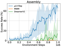
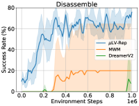
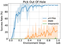
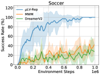
Figure 1: Learning curves on visual robotic manipulation tasks from Meta-world measured by success rate. The solid line and shaded regions represent the mean and standard deviation across five random seeds. Our method shows better or comparable sample efficiency compared to baseline methods. Learning curves on all 50 tasks are reported in Appendix H.

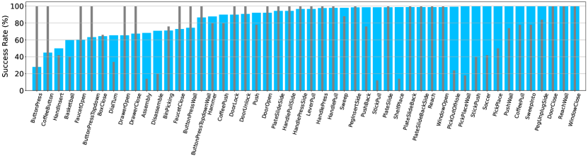
Figure 2: Success Rate on 50 Meta-world tasks after 1 million interactions. The blue bars show our results, the gray bars show the best performance among baselines. Our method succeeds on most of tasks (> 90% on 33 tasks). The results are better than or equivalent to (within 10% difference) the best baselines on 41 tasks.

7 Experimental Evaluation

We evaluate the proposed method on Meta-world (Yu et al., 2019), which is an open-source simulated benchmark consisting of 50 distinct robotic manipulation tasks with visual observations. We also provide experiment results on partial observable control problems constructed based on OpenAI gym MuJoCo (Todorov et al., 2012) in Section H.2.

We notice that directly acquiring a robust control representation through predicting future visual observations can be challenging due to the redundancy of information in images for effective decision-making. As a result, a more advantageous approach involves obtaining an image representation first and subsequently learning a latent representation based on this initial image representation. In particular, we employ visual observations with dimensions of 64 × 64 × 3 and apply a variational autoendocer (VAE) (Kingma and Welling, 2013) to learn a representation of these visual observations. The VAE is trained during the online learning procedure. This produces compact vector representations for the images, which are then forwarded as input to the representation learning method. As detailed in Section 4.2, we learn the latent representations by making predictions about future outcomes using a history of length $L$. To achieve this, we employ a continuous latent variable model similar to (Ren et al., 2023b; Hafner et al., 2020), approximating distributions with Gaussians parameterized by their mean and variance. We then apply Soft Actor-Critic (SAC) as the planner (Haarnoja et al., 2018), which takes the learned representation as input of the critic. We apply $L=3$ across all domains (with an ablation study provided in Section H.1). More implementation details, including network architectures and hyper-parameters, are provided in Appendix H.

We consider two baseline methods, DreamerV2 (Hafner et al., 2021) and the Masked World Model (MWM) (Seo et al., 2023). DreamerV2 is designed to acquire latent representations, which are subsequently input into a recurrent neural network for environment modeling. MWM utilizes an autoencoder equipped with convolutional layers and vision transformers (ViT) rather than reconstructing visual observations. This autoencoder is employed to reconstruct pixels based on masked convolutional features, allowing MWM to learn a latent dynamics model that operates on the representations derived from the autoencoder.

Figure 1 presents the learning curves of all algorithms as measured on the success rate for 1M environment steps, averaged over 5 random seeds. We observe that $\mu$LV-Rep exhibits superior performance compared to both DreamerV2 and MWM, demonstrating faster convergence and achieving higher final performance across all four tasks reported. We also provide the learning curves for all 50 Meta-world tasks in Section H.2. It is noteworthy that while MWM achieves comparable sample efficiency with $\mu$LV-Rep in certain tasks, it incurs higher computational costs and longer running times due to the incorporation of ViT network in its model. In our experimental configurations, $\mu$LV-Rep demonstrates a training speed of 21.3 steps per second, outperforming MWM, which achieves a lower training speed of 8.1 steps per second. This highlights the computational efficiency of the proposed method. Figure 5 illustrates the final performance of $\mu$LV-Rep across 50 Meta-world tasks (blue bars), comparing it with the best performance achieved by DreamerV2 and MWM (gray bars). We observe that $\mu$LV-Rep achieves better than 90% success on 33 tasks. It also performs better or equivalent to (within 10% difference) the best of DreamerV2 and MWM on 41 tasks.

8 Conclusion

In this paper, we aimed to develop a practical RL algorithm for structured POMDPs that obtained efficiency in terms of both statistical and computational complexity. We revealed some of the challenges in computationally exploiting the low-rank structure of a POMDP, then derived a linear representation for the $Q^{\pi}$-function, which automatically implies a practical learning method, with tractable planning and exploration, as in $\mu$LV-Rep. We theoretically analyzed the sub-optimality of the proposed $\mu$LV-Rep, and empirically demonstrated its advantages on several benchmarks.

Appendix

Appendix A More Related Work

Partially Observable RL.

The majority of existing practical RL algorithms for partially observable settings can also be categorized into model-based vs. model-free.

The model-based algorithms [Kaelbling et al., 1998] for partially observed scenarios are naturally derived based on the definition of POMDPs, where both the emission and transition models are learned from data. The planning procedure for optimal policy is conducted over the posterior of latent state, i.e., beliefs, which is approximately inferred based on learned dynamics and emission model. With different model parametrizations, (ranging from Gaussian processes to deep models), and different planning methods, a family of algorithms has been proposed [Deisenroth and Peters, 2012, Igl et al., 2018, Gregor et al., 2019, Zhang et al., 2019, Lee et al., 2020, Hafner et al., 2021]. However, due to the compounding errors from i), mismatch in model parametrization, ii), inaccurate beliefs calculation, iii), approximation in planning over nonlinear dynamics, and iv), neglecting of exploration, such methods might suffer from sub-optimal performances in practice.

As we discussed in Section 1, the memory-based policy and value function have been exploited to extend the MDP-based model-free RL algorithms to handle the non-Markovian dependency induced by partial observations. For example, the value-based algorithms introduces memory-based neural networks to Bellman recursion, including temporal difference learning with explicit concatenation of 4 consecutive frames as input [Mnih et al., 2013] or recurrent neural networks for longer windows [Bakker, 2001, Hausknecht and Stone, 2015, Zhu et al., 2017], and DICE [Nachum and Dai, 2020] with features extracted from transformer [Jiang et al., 2021]; the policy gradient-based algorithms have been extended to partially observable setting by introducing recurrent neural network for policy parametrization [Schmidhuber, 1990, Wierstra et al., 2007, Heess et al., 2015, Ni et al., 2021]. The actor-critic approaches exploits memory-based value and policy together [Ni et al., 2021, Meng et al., 2021]. Despite their simplicity in the algorithm extension, these algorithms demonstrate potentials in real-world applications. However, the it has been observed that the sample complexity for purely model-free RL with partial observations is very high [Mnih et al., 2013, Barth-Maron et al., 2018, Yarats et al., 2021], and the exploration remains difficult, and thus, largely neglected.

Appendix B Observability Approximation

Although the proposed $\mu$LV-Rep is designed based on the $L$-step decodability in POMDPs, Golowich et al. [2022] shows that the $\gamma$-observable POMDPs can be $\epsilon$-approximated with a $L=\tilde{O}\left(\gamma^{-4}\log\left({\left|S\right|}/{\epsilon}\right)\right)$-step decodable POMDP. By exploiting the low-rank structure in the latent dynamics, this result has been extend with function approximator [Uehara et al., 2022]. Specifically,

Theorem 4 (Proprosition 7 [Guo et al., 2023], Lemma 12 [Uehara et al., 2022])

Given a $\gamma$-observable POMDP with $d$-rank latent transition, there exists an $L$-step decodable POMDP $\mathcal{M}$ with $L=\tilde{O}\left(\gamma^{-4}\log\left(d/\epsilon\right)\right)$, $\forall\epsilon>0$, such that

$$\mathbb{E}_{a_{1:h},o_{2:h}\sim\pi}\left[\left\|\mathbb{P}_{h}\left(o_{h+1}|o_{1:h},a_{1:h}\right)-\mathbb{P}_{h}^{\mathcal{M}}\left(o_{h+1}|x_{h},a_{h}\right)\right\|_{1}\right]\leqslant\epsilon.$$ (16)

where $\pi_{h}\in\Delta\left(\prod_{h=1}^{H}\mathcal{A}^{\mathscr{H}_{h}}\right)$ with $\mathscr{H}_{h}:=\mathcal{A}^{h-1}\times\mathcal{O}^{h}$, is mapping the whole history to a distribution of action.

With this understanding, the proposed $\mu$LV-Rep can be directly applied for $\gamma$-observable POMDPs, while still maintains theoretical guarantees. Due to the space limitation, please refer to Uehara et al. [2022], Guo et al. [2023] for the details of the proofs.

Appendix C Moment Matching Policy

We provide a formal definition of the moment matching policy here.

Definition 5 (Moment Matching Policy [Efroni et al., 2022])

With the $L$-decodability assumption, for $h\in[H]$, $h^{\prime}\in[h-L+1,h]$ and $l=h^{\prime}-h+L-1$, we can define the moment matching policy $\nu^{\pi,h}=\{\nu_{h^{\prime}}^{h,\pi}:\mathcal{S}^{l}\times\mathcal{O}^{l}\times\mathcal{A}^{l-1}\to\Delta(\mathcal{A})\}_{h^{\prime}=h-L+1}^{h}$ introduced by Efroni et al. [2022] , such that

$$\nu_{h^{\prime}}^{\pi,h}(a_{h^{\prime}}|(s_{h-L+1:h^{\prime}},o_{h-L+1:h^{\prime}},a_{h-L+1:h^{\prime}-1}))$$

$$\qquad:=\mathbb{E}_{\pi}^{\mathcal{P}}[\pi_{h^{\prime}}(a_{h^{\prime}}|x_{h^{\prime}})|(s_{h-L+1:h^{\prime}},o_{h-L+1:h^{\prime}},a_{h-L+1:h^{\prime}-1})],\quad\forall h^{\prime}\leqslant h-1,$$

and $\nu_{h}^{\pi,h}=\pi_{h}$. We further define $\tilde{\pi}^{h}$, which takes first $h-L$ actions from $\pi$ and the remaining $L$ actions from $\nu^{\pi,h}$.

The main motivation to define such moment matching policy is that, we want to define a policy that is conditionally independent from the past history for theoretical justification while indistinguishable from the history dependent policy to match the practical algorithm. By Lemma B.2 in Efroni et al. [2022], under the $L$-decodability assumption, for a fixed $h\in[H]$, we have $d_{h}^{\mathcal{P},\pi}(x_{h})=d_{h}^{\mathcal{P},\tilde{\pi}_{h}}(x_{h})$, for all $L$-step policy $\pi$ and $x_{h}\in\mathcal{X}_{h}$. As $\nu^{\pi,h}_{h}=\pi_{h}$. we have $d_{h}^{\mathcal{P},\pi}(x_{h},a_{h})=d_{h}^{\mathcal{P},\tilde{\pi}^{h}}(x_{h},a_{h})$, and hence $\mathbb{E}_{\pi}^{\mathcal{P}}(x_{h},a_{h})=\mathbb{E}_{\tilde{\pi}^{h}}^{\mathcal{P}}(x_{h},a_{h})$. This enables the factorization in (10) without the dependency of the overlap observation trajectory.

Appendix D Pessimism in the Offline Setting

Similar to Uehara et al. [2021], Ren et al. [2023b], the proposed algorithm can be directly extended to the offline setting by converting the optimism into the pessimism. Specifically, we can learn the latent variable model, set the penalty with the data and perform planning with the penalized reward. The whole algorithm is shown in Algorithm 2. Following the identical proof strategy from Uehara et al. [2021], Ren et al. [2023b], we can obtain a similar sub-optimal gap guarantee for $\hat{\pi}^{*}$.

Algorithm 2 Offline Learning for $L$-step decodable POMDPs with Latent Variable Representation

1:  Input: Model Class $\mathcal{M}=\{\{(p_{h}(z|x_{h},a_{h}),p_{h}(o_{h+1}|z)\}_{h\in[H]}\}$, Variational Distribution Class $\mathcal{Q}=\{\{q_{h}(z|x_{h},a_{h},o_{h+1})\}_{h\in[H]}\}$, Offline Dataset $\{\mathcal{D}_{h}\}_{h=1}^{H}$

2:  Learn the latent variable model $\hat{p}(z|x_{h},a_{h})$ with $\mathcal{D}_{h}$ via maximizing the ELBO, and obtain the learned model $\widehat{\mathcal{P}}=\{(\hat{p}_{h}(z|x_{h},a_{h}),\hat{p}_{h}(o_{h+1}|z))\}_{h\in[H]}$.

3:  Set the exploitation penalty $\hat{b}_{h}(s,a)$ with $\mathcal{D}_{k}$.

4:  Learn the policy $\hat{\pi}^{*}=\mathop{\arg\max}_{\pi}V^{\pi}_{\widehat{\mathcal{P}},r-\hat{b}_{k}}$.

5:  Return $\hat{\pi}^{*}$.

Appendix E Technical Background

In this section, we revisit several core concepts of the kernel and the reproducing kernel Hilbert space (RKHS) that will be used in the theoretical analysis. For a complete introduction, we refer the reader to Ren et al. [2023b].

Definition 6 (Kernel and Reproducing Kernel Hilbert Space (RKHS))

[Aronszajn, 1950, Paulsen and Raghupathi, 2016] The function $k:\mathcal{X}\times\mathcal{X}\to\mathbb{R}$ is called a kernel on $\mathcal{X}$ if there exists a Hilbert space $\mathcal{H}$ and a mapping $\phi:\mathcal{X}\to\mathcal{H}$ (termed as a feature map), such that $\forall x,x^{\prime}\in\mathcal{X}$, $k(x,x^{\prime})=\langle\phi(x),\phi(x^{\prime})\rangle_{\mathcal{H}}$. The kernel $k$ is said to be positive semi-definite if $\forall n\geqslant 1,\{a_{i}\}_{i\in[n]}\subset\mathbb{R}$ and mutually distinct $\{x_{i}\}_{i\in[n]}$, we have

$$\sum_{i\in[n]}\sum_{j\in[n]}a_{i}a_{j}k(x_{i},x_{j})\geqslant 0.$$

The kernel $k$ is said to be positive definite if the inequality is strict (which means we can replace $\geqslant$ with $>$).

With a given kernel $k$, we can define the Hilbert space $\mathcal{H}_{k}$ consists of $\mathbb{R}$-valued function on $\mathcal{X}$ as a reproducing kernel Hilbert space associated with $k$ if both of the following conditions hold:

• $\forall x\in\mathcal{X}$, $k(x,\cdot)\in\mathcal{H}_{k}$.

• Reproducing Property: $\forall x\in\mathcal{X},f\in\mathcal{H}_{k},f(x)=\langle f,k(x,\cdot)\rangle_{\mathcal{H}_{k}}$.

The RKHS norm of $f\in\mathcal{H}_{k}$ is induced by the inner product, i.e. $\|f\|_{\mathcal{H}_{k}}:=\sqrt{\langle f,f\rangle_{\mathcal{H}_{k}}}$.

Theorem 7 (Mercer’s Theorem [Riesz and Nagy, 2012, Steinwart and Scovel, 2012])

Let $k$ be a continuous positive definite kernel defined on $\mathcal{X}\times\mathcal{X}$. There exists at most countable $\{\mu_{i}\}_{i\in I}$ such that $\mu_{1}\geqslant\mu_{2}\geqslant\cdots>0$ and a set of orthonormal basis $\{e_{i}\}_{i\in I}$ on $L_{2}(\mu)$ where $\mu$ is a Borel measure on $\mathcal{X}$, such that

$$\forall x,x^{\prime}\in\mathcal{X},\quad k(x,x^{\prime})=\sum_{i\in I}\mu_{i}e_{i}(x)e_{i}(x^{\prime}),$$

where the convergence is absolute and uniform.

Definition 8 (Random Feature)

The kernel $k:\mathcal{X}\times\mathcal{X}\to\mathbb{R}$ has a random feature representation if there exists a function $\psi:\mathcal{X}\times\Xi\to\mathbb{R}$ and a probability measure $P$ over $\Xi$ such that

$$k(x,x^{\prime})=\int_{\Xi}\psi(x;\xi)\psi(x^{\prime};\xi)dP(\xi).$$

Remark (random feature quadrature):

We here justify the random feature quadrature [Ren et al., 2023b] for completeness.

We can represent $Q_{h}^{\pi}$ as an expectation,

$$Q_{h}^{\pi}\left(x_{h},a_{h}\right)=\left\langle p(z|x_{h}),w_{h}^{\pi}(z)\right\rangle=\mathbb{E}_{p(z|x_{h})}\left[w_{h}^{\pi}(z)\right]_{L_{2}(\mu)}$$

Under the assumption that $w_{h}^{\pi}(\cdot)\in\mathcal{H}_{k}$, where $\mathcal{H}_{k}$ denoting some RKHS with some kernel $k\left(\cdot,\cdot\right)$. When $k\left(\cdot,\cdot\right)$ can be represented through random feature, i.e.,

$$k\left(x,y\right)=\mathbb{E}_{P(\xi)}\left[\psi\left(x;\xi\right)\psi\left(y;\xi\right)\right],$$

the $w_{h}^{\pi}\left(z\right)$ admits a representation as

$$w_{h}^{\pi}\left(z\right)=\mathbb{E}_{P(\xi)}\left[\tilde{w}^{\pi}_{h}\left(\xi\right)\psi\left(z;\xi\right)\right].$$

Therefore, we plug this random feature representation of $w_{h}^{\pi}(z)$ to $Q_{h}^{\pi}\left(x_{h},a_{h}\right)$, we obtain

$$Q_{h}^{\pi}\left(x_{h},a_{h}\right)=\mathbb{E}_{p(z|x_{h}),P(\xi)}\left[\tilde{w}_{h}^{\pi}(\xi)\psi\left(z;\xi\right)\right].$$ (17)

Applying Monte-Carlo approximation to (17), we obtain the random feature quadrature in (15).

Appendix F Theoretical Analysis

F.1 Technical Conditions

We adopt the following assumptions for the reproducing kernel, which have been used in Ren et al. [2023b] for the MDP setting.

Assumption 3 (Regularity Conditions)

$\mathcal{Z}$ is a compact metric space with respect to the Lebesgue measure $\nu$ when $\mathcal{Z}$ is continuous. Furthermore, $\int_{\mathcal{Z}}k(z,z)d\nu\leqslant 1$.

Assumption 4 (Eigendecay Conditions)

Assume $\{\nu_{i}\}_{i\in I}$ defined in Theorem 7 satisfies one of the following conditions:

• $\beta$-finite spectrum: for some positive integer $\beta$, we have $\nu_{i}=0$, $\forall i>\beta$.

• $\beta$-polynomial decay: $\nu_{i}\leqslant C_{0}i^{-\beta}$ with absolute constant $C_{0}$ and $\beta>1$.

• $\beta$-exponential decay: $\nu_{i}\leqslant C_{1}\exp(-C_{2}i^{\beta})$, with absolute constants $C_{1}$, $C_{2}$ and $\beta>0$.

We will use $C_{\mathrm{poly}}$ to denote constants in the analysis of $\beta$-polynomial decay that only depends on $C_{0}$ and $\beta$, and $C_{\mathrm{exp}}$ to denote constants in the analysis of $\beta$-exponential decay that only depends on $C_{1}$, $C_{2}$ and $\beta$, to simplify the dependency of the constant terms. Both of $C_{\mathrm{poly}}$ and $C_{\mathrm{exp}}$ can be varied step by step.

F.2 Formal Proof

Before we proceed, we first define

$$\rho_{k,h}=\frac{1}{k}\sum_{i\in[K]}d_{\mathcal{P},h}^{\pi_{k}},$$

and $\circ^{L}\mathcal{U}(\mathcal{A})$ means uniformly taking actions in the consecutive $L$ steps.

Lemma 9 ($L$-step back inequality for the true model)

Given a set of functions $\left[g_{h}\right]_{h\in[H]}$, where $g_{h}:\mathcal{X}\times\mathcal{A}\to\mathbb{R}$, $\|g_{h}\|_{\infty}\leqslant B$, $\forall h\in[H]$, we have that $\forall\pi$,

$$\sum_{h\in[H]}\mathbb{E}_{\pi}^{\mathcal{P}}[g(x_{h},a_{h})]\leqslant \sum_{h\in[H]}\mathbb{E}_{(x_{h-L},a_{h-L})\sim d_{\mathcal{P},h-L}^{\pi}}^{\mathcal{P}}\left[\left\|p^{*}(\cdot|x_{h-L},a_{h-L})\right\|_{L_{2}(\mu),\Sigma_{\rho_{k,h-L},p^{*}}^{-1}}\right]$$

$$\cdot\sqrt{k|\mathcal{A}|^{L}\cdot\mathbb{E}_{(\tilde{x}_{h},\tilde{a}_{h})\sim\rho_{k,h-L}\circ^{L}\mathcal{U}(\mathcal{A})}\left[g(\tilde{x}_{h},\tilde{a}_{h})^{2}\right]+\lambda B^{2}C}$$

Proof  The proof can be adapted from the proof of Lemma 6 in Ren et al. [2023b], and we include it for the completeness. Recall the moment matching policy $\nu^{\pi}$ Since $\nu^{\pi,h}$ does not depend on $(x_{h-L},a_{h-L})$, we can make the following decomposition:

$$\mathbb{E}_{\tilde{\pi}^{h}}^{\mathcal{P}}(x_{h},a_{h})$$

$$= \mathbb{E}_{(x_{h-L},a_{h-L})\sim\pi}^{\mathcal{P}}\left[\int_{s_{h-L+1}}\langle p^{*}(\cdot|x_{h-L},a_{h-L}),p^{*}(s_{h-L+1}|\cdot)\rangle_{L_{2}(\mu)}\cdot\mathbb{E}_{a_{h-L+1:h\sim\nu^{\pi,h}}}^{\mathcal{P}}[g(x_{h},a_{h})|s_{h-L+1}]ds_{h-L+1}\right]$$

$$\leqslant \mathbb{E}_{(x_{h-L},a_{h-L})\sim\pi}^{\mathcal{P}}\left\|p^{*}(\cdot|x_{h-L},a_{h-L})\right\|_{L_{2}(\mu),\Sigma_{\rho_{k,h-L},p^{*}}^{-1}}$$

$$\cdot\left\|\int_{s_{h-L+1}}p^{*}(s_{h-L+1}|\cdot)\mathbb{E}[g(x_{h},a_{h})|s_{h-L+1},\nu^{\pi,h}]ds_{h-L+1}\right\|_{L_{2}(\mu),\Sigma_{\rho_{k,h-L},p^{*}}}.$$

Direct computation shows that

$$\left\|\int_{s_{h-L+1}}p^{*}(s_{h-L+1}|\cdot)\mathbb{E}^{\mathcal{P}}[g(x_{h},a_{h})|s_{h-L+1},\nu^{\pi,h}]ds_{h-L+1}\right\|_{L_{2}(\mu),\Sigma_{\rho_{k,h-L},p^{*}}}$$

$$= k\mathbb{E}_{(\tilde{x}_{h-L},\tilde{a}_{h-L})\sim\rho_{k,h-L}}\left[\mathbb{E}_{s_{h-L+1}\sim\mathbb{P}_{h-L}^{\mathcal{P}}(\cdot|x_{h-L},a_{h-L})}^{\mathcal{P}}[g(x_{h},a_{h})|s_{h-L+1},\nu^{\pi,h}]\right]^{2}$$

$$+\left\|\int_{s_{h-L+1}}p^{*}(s_{h-L+1}|\cdot)\cdot\mathbb{E}^{\mathcal{P}}[g(x_{h},a_{h})|s_{h-L+1},\nu^{\pi,h}]ds_{h-L+1}\right\|_{\mathcal{H}}^{2}$$

$$\leqslant k\mathbb{E}_{(\tilde{x}_{h-L},\tilde{a}_{h-L})\sim\rho_{k,h-L}}\mathbb{E}^{\mathcal{P}}_{s_{h-L+1}\sim\mathbb{P}_{h-L}^{\mathcal{P}}(\cdot|x_{h-L},a_{h-L}),a_{h-L+1:h}\sim\nu^{\pi,h}}\left[g(x_{h},a_{h})\right]^{2}+\lambda B^{2}C$$

$$\leqslant k|\mathcal{A}|^{L}\mathbb{E}^{\mathcal{P}}_{(\tilde{x}_{h},\tilde{a}_{h})\sim\rho_{k,h-L}\circ^{L}\mathcal{U}(\mathcal{A})}[g(\tilde{x}_{h},\tilde{a}_{h})]^{2}+\lambda B^{2}C,$$

which finishes the proof.  

Lemma 10 ($L$-step back inequality for the learned model)

Assume we have a set of functions $\left[g_{h}\right]_{h\in[H]}$, where $g_{h}:\mathcal{X}\times\mathcal{A}\to\mathbb{R}$, $\|g_{h}\|_{\infty}\leqslant B$, $\forall h\in[H]$. Given Lemma 15, we have that $\forall\pi$,

$$\sum_{h\in[H]}\mathbb{E}_{\pi}^{\widehat{\mathcal{P}}_{k}}[g(x_{h},a_{h})]\leqslant \sum_{h\in[H]}\mathbb{E}_{(x_{h-L},a_{h-L})\sim d_{\widehat{\mathcal{P}}_{k},h-L}^{\pi}]}^{\widehat{\mathcal{P}}_{k}}\left[\left\|\hat{p}(\cdot|x_{h-L},a_{h-L})\right\|_{L_{2}(\mu),\Sigma_{\rho_{k,h-2L}\circ^{L}\mathcal{U}(\mathcal{A}),\hat{p}}^{-1}}\right]$$

$$\cdot\sqrt{k|\mathcal{A}|^{L}\cdot\mathbb{E}_{(\tilde{x}_{h},\tilde{a}_{h})\sim\rho_{k,h-2L}\circ^{2L}\mathcal{U}(\mathcal{A})}\left[g(\tilde{x}_{h},\tilde{a}_{h})^{2}\right]+\lambda B^{2}C+kL|\mathcal{A}|^{L-1}B^{2}\zeta_{k}}$$

Proof  The proof can be adapted from the proof of Lemma 5 in Ren et al. [2023b], and we include it for the completeness. We define a similar moment matching policy and make the following decomposition:

$$\mathbb{E}_{\pi}^{\widehat{\mathcal{P}}_{k}}(x_{h},a_{h})$$

$$= \mathbb{E}_{(x_{h-L},a_{h-L})\sim\pi}^{\widehat{\mathcal{P}}_{k}}\left[\int_{s_{h-L+1}}\langle\hat{p}(\cdot|x_{h-L},a_{h-L}),\hat{p}(s_{h-L+1}|\cdot)\rangle_{L_{2}(\mu)}\cdot\mathbb{E}^{\widehat{\mathcal{P}}_{k}}[g(x_{h},a_{h})|s_{h-L+1},\nu^{\pi,h}]ds_{h-L+1}\right]$$

$$\leqslant \mathbb{E}_{(x_{h-L},a_{h-L})\sim\pi}^{\widehat{\mathcal{P}}_{k}}\left\|\hat{p}(\cdot|x_{h-L},a_{h-L})\right\|_{L_{2}(\mu),\Sigma_{\rho_{k,h-2L}\circ^{L}\mathcal{U}(\mathcal{A}),\hat{p}}^{-1}}$$

$$\cdot\left\|\int_{s_{h-L+1}}\hat{p}(s_{h-L+1}|\cdot)\mathbb{E}^{\widehat{\mathcal{P}}_{k}}[g(x_{h},a_{h})|s_{h-L+1},\nu^{\pi,h}]ds_{h-L+1}\right\|_{L_{2}(\mu),\Sigma_{\rho_{k,h-2L}\circ^{L}\mathcal{U}(\mathcal{A}),\hat{p}}}.$$

Direct computation shows that

$$\left\|\int_{s_{h-L+1}}\hat{p}(s_{h-L+1}|\cdot)\mathbb{E}^{\widehat{\mathcal{P}}_{k}}[g(x_{h},a_{h})|s_{h-L+1},\nu^{\pi,h}]ds_{h-L+1}\right\|_{L_{2}(\mu),\Sigma_{\rho_{k,h-2L}\circ^{L}\mathcal{U}(\mathcal{A}),\hat{p}}}^{2}$$

$$= k\mathbb{E}_{(\tilde{x}_{h-L},\tilde{a}_{h-L})\sim\rho_{k,h-2L}\circ^{L}\mathcal{U}(\mathcal{A})}\left[\mathbb{E}_{s_{h-L+1}\sim\mathbb{P}_{h-L}^{\widehat{\mathcal{P}}_{k}}(\cdot|\tilde{x}_{h-L},\tilde{a}_{h-L})}\mathbb{E}^{\widehat{\mathcal{P}}_{k}}[g(x_{h},a_{h})|s_{h-L+1},\nu^{\pi,h}]\right]^{2}$$

$$+\left\|\int_{s_{h-L+1}}\hat{p}(s_{h-L+1}|\cdot)\mathbb{E}[g(x_{h},a_{h})|s_{h-L+1},\nu^{\pi,h}]ds_{h-L+1}\right\|_{\mathcal{H}}^{2}$$

$$\leqslant k\mathbb{E}_{(\tilde{x}_{h-L},\tilde{a}_{h-L})\sim\rho_{k,h-2L}\circ^{L}\mathcal{U}(\mathcal{A})}\mathbb{E}_{s_{h-L+1}\sim\mathbb{P}_{h-L}^{\widehat{\mathcal{P}}_{k}}(\cdot|\tilde{x}_{h-L},\tilde{a}_{h-L}),\nu^{\pi,h}}^{\widehat{\mathcal{P}}_{k}}[g(x_{h},a_{h})]^{2}+\lambda B^{2}C$$

$$\leqslant k|\mathcal{A}|^{L}\mathbb{E}_{(\tilde{x}_{h-L},\tilde{a}_{h-L})\sim\rho_{k,h-2L}\circ^{L}\mathcal{U}(\mathcal{A})}\mathbb{E}^{\widehat{\mathcal{P}}_{k}}_{a_{h-L+1:h}\sim\circ^{L}\mathcal{U}(\mathcal{A})}[g(x_{h},a_{h})]^{2}+\lambda B^{2}C$$

$$\leqslant k|\mathcal{A}|^{L}\mathbb{E}_{(\tilde{x}_{h},\tilde{a}_{h})\sim\rho_{k,h-2L}\circ^{2L}\mathcal{U}(\mathcal{A})}[g(\tilde{x}_{h},\tilde{a}_{h})]^{2}+kL|\mathcal{A}|^{L-1}B^{2}\zeta_{k}+\lambda B^{2}C,$$

where we use the MLE guarantee for each individual step to obtain the last inequality. This finishes the proof.  

Lemma 11 (Almost Optimism)

For episode $k\in[K]$, set

$$\hat{b}_{k,h}=\min\left\{\alpha_{k}\|\hat{p}_{k}(\cdot|x_{h-L},a_{h-L})\|_{L_{2}(\mu),\hat{\Sigma}_{k,h,\hat{p}_{k}}^{-1}},2\right\},$$

with $\alpha_{k}=\frac{\sqrt{5kL|\mathcal{A}|^{L}\zeta_{k}+4\lambda d}}{c}$,

$$\hat{\Sigma}_{k,h,\hat{p}_{k}}:L_{2}(\mu)\to L_{2}(\mu),\quad\hat{\Sigma}_{k,h,\hat{p}_{k}}:=\sum_{(x_{h,i},a_{h,i})\in\mathcal{D}_{k,h}}\left[\hat{p}_{k}(z|x_{h,i},a_{h,i})\hat{p}_{k}(z|x_{h,i},a_{h,i})^{\top}\right]+\lambda T_{K}^{-1}$$

where $T_{K}$ is the integral operator associated with $K$ (i.e. $T_{K}f=\int f(x)K(x,\cdot)dx$) and $\lambda$ is set for different eigendecay of $K$ as follows:

• $\beta$-finite spectrum: $\lambda=\Theta(\beta\log K+\log(K|\mathcal{P}|/\delta))$

• $\beta$-polynomial decay: $\lambda=\Theta(C_{\mathrm{poly}}K^{1/(1+\beta)}+\log(K|\mathcal{P}|/\delta))$;

• $\beta$-exponential decay: $\lambda=\Theta(C_{\mathrm{exp}}(\log K)^{1/\beta}+\log(K|\mathcal{P}|/\delta))$;

$c$ is an absolute constant, then with probability at least $1-\delta$, $\forall k\in[K]$ we have

$$V^{\pi^{*},\widehat{\mathcal{P}}_{k},r+\widehat{b}_{k}}-V^{\pi^{*},\mathcal{P},r}\geqslant-\sqrt{|\mathcal{A}|^{L+1}\zeta_{k}}$$

Proof  With Lemma 14, we have that

$$V^{\pi^{*},\widehat{\mathcal{P}}_{k},r+\widehat{b}^{k}}-V^{\pi^{*},\mathcal{P},r}$$

$$= \sum_{h\in[H]}\mathbb{E}_{(x_{h},a_{h})\sim d_{\widehat{\mathcal{P}}_{k},h}^{\pi^{*}}}\left[\widehat{b}_{h}^{k}(x_{h},a_{h})+\mathbb{E}_{o^{\prime}\sim\mathbb{P}_{h}^{\widehat{\mathcal{P}}_{k}}(\cdot|x_{h},a_{h})}[V_{h+1}^{\pi^{*},\mathcal{P},r}(x_{h+1}^{\prime})]-\mathbb{E}_{o^{\prime}\sim\mathbb{P}_{h}^{\mathcal{P}}(\cdot|x_{h},a_{h})}[V_{h+1}^{\pi^{*},\mathcal{P},r}(x_{h+1}^{\prime})]\right]$$

$$\geqslant \sum_{h\in[H]}\mathbb{E}_{(x_{h},a_{h})\sim d_{\widehat{\mathcal{P}}_{k},h}^{\pi^{*}}}\left[\min\left[c\alpha_{k}\left\|\hat{p}(\cdot|x_{h-L},a_{h-L})\right\|_{L_{2}(\mu),\Sigma_{\rho_{k,h-L},\hat{p}}^{-1}},2\right]+\mathbb{E}_{o^{\prime}\sim\mathbb{P}_{h}^{\widehat{\mathcal{P}}_{k}}(\cdot|x_{h},a_{h})}[V_{h+1}^{\pi^{*},\mathcal{P},r}(x_{h+1}^{\prime})]\right.$$

$$\left.-\mathbb{E}_{o^{\prime}\sim\mathbb{P}_{h}^{\mathcal{P}}(\cdot|x_{h},a_{h})}[V_{h+1}^{\pi^{*},\mathcal{P},r}(x_{h+1}^{\prime})]\right],$$

where in the last step we replace the empirical covariance with the population counterpart thanks to Lemma 17 in Ren et al. [2023b]. Define

$$g_{h}(z_{h},a_{h})=\mathbb{E}_{o^{\prime}\sim\mathbb{P}_{h}^{\mathcal{P}}(\cdot|x_{h},a_{h})}[V_{h+1}^{\pi^{*},\mathcal{P},r}(x_{h+1}^{\prime})]-\mathbb{E}_{o^{\prime}\sim\mathbb{P}_{h}^{\widehat{\mathcal{P}}_{k}}(\cdot|x_{h},a_{h})}[V_{h+1}^{\pi^{*},\mathcal{P},r}(x_{h+1}^{\prime})],$$

With Hölder’s inequality, we have that $\|g_{h}\|_{\infty}\leqslant 2$.

Furthermore, with Lemma 10, we have that

$$\sum_{h\in[H]}\mathbb{E}_{(x_{h},a_{h})\sim d_{\widehat{\mathcal{P}}_{k},h}^{\pi^{*}}}[g_{h}(x_{h},a_{h})]$$

$$\leqslant \sum_{h\in[H]}\mathbb{E}_{(x_{h-L},a_{h-L})\sim d_{\widehat{\mathcal{P}}_{k},h}^{\pi^{*}}}\left[\left\|\hat{p}(\cdot|x_{h-L},a_{h-L})\right\|_{L_{2}(\mu),\Sigma_{\rho_{k,h-L},\hat{p}}^{-1}}\right]$$

$$\cdot\sqrt{k|\mathcal{A}|^{L}\cdot\mathbb{E}_{(\tilde{x}_{h},\tilde{a}_{h})\sim\rho_{h-2L}\circ^{2L}\mathcal{U}(\mathcal{A})}\left[g(\tilde{x}_{h},\tilde{a}_{h})^{2}\right]+4\lambda C+4kL|\mathcal{A}|^{L-1}\zeta_{k}}$$

$$\leqslant \sum_{h\in[H]}\mathbb{E}_{(x_{h-L},a_{h-L})\sim d_{\widehat{\mathcal{P}}_{k},h}^{\pi^{*}}}\left[c\alpha_{k}\left\|\hat{p}(\cdot|x_{h-L},a_{h-L})\right\|_{L_{2}(\mu),\Sigma_{\rho_{k,h-L},\hat{p}}^{-1}}\right],$$

where we use Lemma 15 in the last step. Now we deal with the case with $h\in[L]$. Note that, $\forall h\in[L]$

$$\mathbb{E}_{(x_{h},a_{h})\sim\pi}[g_{h}(x_{h},a_{h})]$$

$$\leqslant |\mathcal{A}|^{h}\mathbb{E}_{x_{1}\sim d_{1},a_{1:h}\sim\circ^{h}\mathcal{U}(\mathcal{A})}\left\|\mathbb{P}^{\widehat{\mathcal{P}}_{k}}_{h}(\cdot|x_{h},a_{h})-\mathbb{P}^{\mathcal{{P}}}_{h}(\cdot|x_{h},a_{h})\right\|_{1}$$

$$\leqslant \sqrt{\mathbb{E}_{x_{1}\sim d_{1},a_{1:h}\circ^{L}\mathcal{U}(\mathcal{A})}\left\|\mathbb{P}^{\widehat{\mathcal{P}}_{k}}_{h}(\cdot|x_{h},a_{h})-\mathbb{P}^{\mathcal{{P}}}_{h}(\cdot|x_{h},a_{h})\right\|_{1}^{2}}$$

$$\leqslant \sqrt{|\mathcal{A}|^{h}\zeta_{k}},$$

where in the last step we use Lemma 15. We finish the proof by summing over $h\in[L]$.  

Lemma 12 (Regret)

With probability at least $1-\delta$, we have that

• For $\beta$-finite spectrum, we have

  $$\sum_{k=1}^{K}V^{\pi^{*},\mathcal{P},r}-V^{\pi_{k},\mathcal{P},r}\lesssim\sum_{k=1}^{K}V^{\pi^{*},\mathcal{P},r}-V^{\pi_{k},\mathcal{P},r}\lesssim H^{2}\beta^{3/2}|\mathcal{A}|^{L}\log K\sqrt{CLK\log(K|\mathcal{M}|/\delta)};$$

• For $\beta$-polynomial decay, we have

  $$\sum_{k=1}^{K}V^{\pi^{*},\mathcal{P},r}-V^{\pi_{k},\mathcal{P},r}\lesssim C_{\mathrm{poly}}H^{2}|\mathcal{A}|^{L}K^{\frac{1}{2}+\frac{1}{1+\beta}}\sqrt{CL\log(K|\mathcal{M}|/\delta)};$$

• For $\beta$-exponential decay, we have

  $$\sum_{k=1}^{K}V^{\pi^{*},\mathcal{P},r}-V^{\pi_{k},\mathcal{P},r}\lesssim C_{\mathrm{exp}}H^{2}|\mathcal{A}|^{L}(\log K)^{1+\frac{3}{2\beta}}\sqrt{CLK\log(K|\mathcal{M}|/\delta)};$$

Proof  With Lemma 11 and Lemma 14, we have

$$V^{\pi^{*},\mathcal{P},r}-V^{\pi_{k},\mathcal{P},r}$$

$$\leqslant V^{\pi^{*},\widehat{\mathcal{P}}_{k},r+\widehat{b}^{k}}+\sqrt{|\mathcal{A}|^{L+1}\zeta_{k}}-V^{\pi_{k},\mathcal{P},r}$$

$$\leqslant V^{\pi^{k},\widehat{\mathcal{P}}_{k},r+\widehat{b}^{k}}+\sqrt{|\mathcal{A}|^{L+1}\zeta_{k}}-V^{\pi_{k},\mathcal{P},r}$$

$$= \sum_{h\in[H]}\mathbb{E}_{(x_{h},a_{h})\sim d_{\mathcal{P},h}^{\pi_{k}}}\left[\widehat{b}_{h}^{k}(x_{h},a_{h})+\mathbb{E}_{o^{\prime}\sim\mathbb{P}_{h}^{\widehat{\mathcal{P}}_{k}}(\cdot|x_{h},a_{h})}\left[V_{h+1}^{\pi_{k},\widehat{\mathcal{P}}_{k},r+\widehat{b}_{h}^{k}}(x_{h+1}^{\prime})\right]-\mathbb{E}_{o^{\prime}\sim\mathbb{P}_{h}^{\mathcal{P}}(\cdot|x_{h},a_{h})}\left[V_{h+1}^{\pi_{k},\widehat{\mathcal{P}}_{k},r+\widehat{b}_{h}^{k}}(x_{h+1}^{\prime})\right]\right],$$

$$+\sqrt{|\mathcal{A}|^{L+1}\zeta_{k}}.$$

Note that $\left\|\widehat{b}_{h}^{k}\right\|_{\infty}\leqslant 2$. Applying Lemma 9, we have that

$$\sum_{h\in[H]}\mathbb{E}_{(x_{h},a_{h})\sim d_{\mathcal{P},h}^{\pi_{k}}}\left[\widehat{b}_{h}^{k}(x_{h},a_{h})\right]$$

$$\leqslant \sum_{h\in[H]}\mathbb{E}_{(\tilde{x}_{h-L},\tilde{a}_{h-L})\sim d_{\mathcal{P},h}^{\pi_{k}}}\left[\left\|p^{*}(\cdot|x_{h-L},a_{h-L})\right\|_{L_{2}(\mu),\Sigma_{\rho_{k,h-L},p^{*}}^{-1}}\right]$$

$$\cdot\sqrt{k|\mathcal{A}|^{L}\cdot\mathbb{E}_{(\tilde{x}_{h},\tilde{a}_{h})\sim\rho_{k,h-L}\circ^{L}\mathcal{U}(\mathcal{A})}\left[\widehat{b}_{h}^{k}(\tilde{x}_{h},\tilde{a}_{h})^{2}\right]+4\lambda C}$$

Following the proof of Lemma 8 in Ren et al. [2023b], we have that:

• for $\beta$-finite spectrum,

  $$k\mathbb{E}_{(\tilde{x}_{h},\tilde{a}_{h})\sim\rho_{k,h-L}\circ^{L}\mathcal{U}(\mathcal{A})}\left[\widehat{b}_{h}^{k}(\tilde{x}_{h},\tilde{a}_{h})^{2}\right]=O(\beta\log K);$$

• for $\beta$-polynomial decay,

  $$k\mathbb{E}_{(\tilde{x}_{h},\tilde{a}_{h})\sim\rho_{k,h-L}\circ^{L}\mathcal{U}(\mathcal{A})}\left[\widehat{b}_{h}^{k}(\tilde{x}_{h},\tilde{a}_{h})^{2}\right]=O\left(C_{\mathrm{poly}}K^{\frac{1}{2(1+\beta)}}\log K\right);$$

• for $\beta$-exponential decay,

  $$k\mathbb{E}_{(\tilde{x}_{h},\tilde{a}_{h})\sim\rho_{k,h-L}\circ^{L}\mathcal{U}(\mathcal{A})}\left[\widehat{b}_{h}^{k}(\tilde{x}_{h},\tilde{a}_{h})^{2}\right]=O\left(C_{\mathrm{exp}}(\log K)^{1+1/\beta}\right).$$

We then consider

$$\sum_{h\in[H]}\mathbb{E}_{(x_{h},a_{h})\sim d_{\mathcal{P},h}^{\pi_{k}}}\left[\mathbb{E}_{o^{\prime}\sim\mathbb{P}_{h}^{\widehat{\mathcal{P}}_{k}}(\cdot|x_{h},a_{h})}\left[V_{h+1}^{\pi_{k},\widehat{\mathcal{P}}_{k},r+\widehat{b}_{h}^{k}}(x_{h+1}^{\prime})\right]-\mathbb{E}_{o^{\prime}\sim\mathbb{P}_{h}^{\mathcal{P}}(\cdot|x_{h},a_{h})}\left[V_{h+1}^{\pi_{k},\widehat{\mathcal{P}}_{k},r+\widehat{b}_{h}^{k}}(x_{h+1}^{\prime})\right]\right].$$

Define

$$g(x_{h},a_{h})=\frac{1}{2H+1}\left[\mathbb{E}_{o^{\prime}\sim\mathbb{P}_{h}^{\widehat{\mathcal{P}}_{k}}(\cdot|x_{h},a_{h})}\left[V_{h+1}^{\pi_{k},\widehat{\mathcal{P}}_{k},r+\widehat{b}_{h}^{k}}(x_{h+1}^{\prime})\right]-\mathbb{E}_{o^{\prime}\sim\mathbb{P}_{h}^{\mathcal{P}}(\cdot|x_{h},a_{h})}\left[V_{h+1}^{\pi_{k},\widehat{\mathcal{P}}_{k},r+\widehat{b}_{h}^{k}}(x_{h+1}^{\prime})\right]\right].$$

With Hölder’s inequality and note that $\left\|\widehat{b}_{h}^{k}\right\|\leqslant 2$, we have that $\|g\|_{\infty}\leqslant 2$. With Lemma 9, we have that

$$\sum_{h\in[H]}\mathbb{E}_{(x_{h},a_{h})\sim d_{\mathcal{P},h}^{\pi_{k}}}[g(x_{h},a_{h})]$$

$$\leqslant \sum_{h\in[H]}\mathbb{E}_{(x_{h-L},a_{h-L})\sim d_{\mathcal{P},h}^{\pi_{k}}}^{\mathcal{P}}\left[\left\|p^{*}(\cdot|x_{h-L},a_{h-L})\right\|_{L_{2}(\mu),\Sigma_{\rho_{k,h-L},p^{*}}^{-1}}\right]\cdot\sqrt{k|\mathcal{A}|^{L}\mathbb{E}_{(\tilde{x}_{h},\tilde{a}_{h})\sim\rho_{k,h-L}\circ^{L}\mathcal{U}(\mathcal{A})}\left[g(\tilde{x}_{h},\tilde{a}_{h})^{2}\right]+4\lambda C}$$

$$\leqslant \sum_{h\in[H]}\mathbb{E}_{(x_{h-L},a_{h-L})\sim d_{\mathcal{P},h}^{\pi_{k}}}^{\mathcal{P}}\left[\left\|p^{*}(\cdot|x_{h-L},a_{h-L})\right\|_{L_{2}(\mu),\Sigma_{\rho_{k,h-L},p^{*}}^{-1}}\right]\cdot\sqrt{k|\mathcal{A}|^{L}\zeta_{k}+4\lambda C}$$

$$\leqslant c\alpha_{k}\sum_{h\in[H]}\mathbb{E}_{(x_{h-L},a_{h-L})\sim d_{\mathcal{P},h}^{\pi}}^{\mathcal{P}}\left[\left\|p^{*}(\cdot|x_{h-L},a_{h-L})\right\|_{L_{2}(\mu),\Sigma_{\rho_{k,h-L},p^{*}}^{-1}}\right]$$

With Cauchy-Schwartz inequality, we know that

$$\sum_{k\in[K]}\mathbb{E}_{(x_{h-L},a_{h-L})\sim d_{\mathcal{P},h}^{\pi_{k}}}^{\mathcal{P}}\left[\left\|p^{*}(\cdot|x_{h-L},a_{h-L})\right\|_{L_{2}(\mu),\Sigma_{\rho_{k,h-L},p^{*}}^{-1}}\right]$$

$$\leqslant \sqrt{K\sum_{k\in[K]}\mathbb{E}_{(x_{h-L},a_{h-L})\sim d_{\mathcal{P},h}^{\pi_{k}}}^{\mathcal{P}}\left[\left\|p^{*}(\cdot|x_{h-L},a_{h-L})\right\|_{L_{2}(\mu),\Sigma_{\rho_{k,h-L},p^{*}}^{-1}}^{2}\right]}.$$

Following the proof of Lemma 8 in Ren et al. [2023b], we have that

• for $\beta$-finite spectrum,

  $$\sum_{k\in[K]}\mathbb{E}_{(x_{h-L},a_{h-L})\sim d_{\mathcal{P},h}^{\pi_{k}}}^{\mathcal{P}}\left[\left\|p^{*}(\cdot|x_{h-L},a_{h-L})\right\|_{L_{2}(\mu),\Sigma_{\rho_{k,h-L},p^{*}}^{-1}}^{2}\right]=O(\beta\log K);$$

• for $\beta$-polynomial decay,

  $$\sum_{k\in[K]}\mathbb{E}_{(x_{h-L},a_{h-L})\sim d_{\mathcal{P},h}^{\pi_{k}}}^{\mathcal{P}}\left[\left\|p^{*}(\cdot|x_{h-L},a_{h-L})\right\|_{L_{2}(\mu),\Sigma_{\rho_{k,h-L},p^{*}}^{-1}}^{2}\right]=O\left(C_{\mathrm{poly}}K^{\frac{1}{2(1+\beta)}}\log K\right);$$

• for $\beta$-exponential decay,

  $$\sum_{k\in[K]}\mathbb{E}_{(x_{h-L},a_{h-L})\sim d_{\mathcal{P},h}^{\pi_{k}}}^{\mathcal{P}}\left[\left\|p^{*}(\cdot|x_{h-L},a_{h-L})\right\|_{L_{2}(\mu),\Sigma_{\rho_{k,h-L},p^{*}}^{-1}}^{2}\right]=O\left(C_{\mathrm{exp}}(\log K)^{1+1/\beta}\right).$$

Combine the previous steps and take the dominating term out, we have that

• for $\beta$-finite spectrum,

  $$\sum_{k=1}^{K}V^{\pi^{*},\mathcal{P},r}-V^{\pi_{k},\mathcal{P},r}\lesssim H^{2}\beta^{3/2}|\mathcal{A}|^{L}\log K\sqrt{CLK\log(K|\mathcal{M}|/\delta)};$$

• for $\beta$-polynomial decay,

  $$\sum_{k=1}^{K}V^{\pi^{*},\mathcal{P},r}-V^{\pi_{k},\mathcal{P},r}\lesssim C_{\mathrm{poly}}H^{2}|\mathcal{A}|^{L}K^{\frac{1}{2}+\frac{1}{1+\beta}}\sqrt{CL\log(K|\mathcal{M}|/\delta)};$$

• for $\beta$-exponential decay,

  $$\sum_{k=1}^{K}V^{\pi^{*},\mathcal{P},r}-V^{\pi_{k},\mathcal{P},r}\lesssim C_{\mathrm{exp}}H^{2}|\mathcal{A}|^{L}(\log K)^{1+\frac{3}{2\beta}}\sqrt{CLK\log(K|\mathcal{M}|/\delta)};$$

which finishes the proof.  

Theorem 13 (PAC Guarantee)

After interacting with the environments for $KH$ episodes

• $K=\Theta\left(\frac{CH^{4}L\beta^{3}|\mathcal{A}|^{2L}\log(|\mathcal{P}|/\delta)}{\varepsilon^{2}}\log^{3}\left(\frac{CH^{4}L\beta^{3}|\mathcal{A}|^{2L}\log(|\mathcal{P}|/\delta)}{\varepsilon^{2}}\right)\right)$ for $\beta$-finite spectrum;

• $K=\Theta\left(C_{\mathrm{poly}}\left(\frac{H^{2}L|\mathcal{A}|^{L}\sqrt{C\log(|\mathcal{P}|/\delta)}}{\varepsilon}\log^{3/2}\left(\frac{\sqrt{C}H^{2}L|\mathcal{A}|^{L}\log(|\mathcal{P}|/\delta)}{\varepsilon}\right)\right)^{\frac{2(1+\beta)}{\beta-1}}\right)$ for $\beta$-polynomial decay;

• $K=\Theta\left(\frac{C_{\mathrm{exp}}CH^{4}L|\mathcal{A}|^{2L}\log(|\mathcal{P}|/\delta)}{\varepsilon^{2}}\log^{\frac{3+2\beta}{\beta}}\left(\frac{CH^{4}L|\mathcal{A}|^{2L}\log(|\mathcal{P}|/\delta)}{\varepsilon^{2}}\right)\right)$ for $\beta$-exponential decay;

we can obtain an $\varepsilon$-optimal policy with high probability.

Proof  This is a direct extension of the proof of Theorem 9 in Ren et al. [2023b].  

Appendix G Technical Lemma

Lemma 14 (Simulation Lemma)

For two MDPs $\mathcal{M}=(P,r)$ and $\mathcal{M}^{\prime}=(P^{\prime},r+b)$, we have

$$V_{P^{\prime},r+b}^{\pi}-V_{P,r}^{\pi}$$

$$= \sum_{h\in[H]}\mathbb{E}_{(s_{h},a_{h})\sim d_{P,\pi}^{h}}\left[b_{h}(s_{h},a_{h})+\mathbb{E}_{s_{h+1}\sim P^{\prime}(s_{h},a_{h})}\left[V_{P^{\prime},r+b,h+1}^{\pi}(s_{h+1})\right]-\mathbb{E}_{s_{h+1}\sim P(s_{h},a_{h})}\left[V_{P^{\prime},r+b,h+1}^{\pi}(s_{h+1})\right]\right],$$

and

$$V_{P^{\prime},r+b}^{\pi}-V_{P,r}^{\pi}$$

$$= \sum_{h\in[H]}\mathbb{E}_{(s_{h},a_{h})\sim d_{P^{\prime},\pi}^{h}}\left[b_{h}(s_{h},a_{h})+\mathbb{E}_{s_{h+1}\sim P^{\prime}(s_{h},a_{h})}\left[V_{P,r,h+1}^{\pi}(s_{h+1})\right]-\mathbb{E}_{s_{h+1}\sim P(s_{h},a_{h})}\left[V_{P,r,h+1}^{\pi}(s_{h+1})\right]\right],$$

For the proof, see Uehara et al. [2021] for an example.

Lemma 15 (MLE Guarantee)

For any episoode $k\in[K]$, step $h\in[H]$, define $\rho_{h}$ as the joint distribution of $(x_{h},a_{h})$ in the dataset $\mathcal{D}_{h,k}$ at episode $k$. Then with probability at least $1-\delta$, we have that

$$\mathbb{E}_{(x_{h},a_{h})\sim\mathcal{D}_{h,k}}\left\|\mathbb{P}_{h}^{\mathcal{P}}(\cdot|x_{h},a_{h})-\mathbb{P}_{h}^{\widehat{\mathcal{P}}_{k}}(\cdot|x_{h},a_{h})\right\|_{1}^{2}\leqslant\zeta_{k},$$

where $\zeta_{k}=O(\log(Hk|\mathcal{M}|/\delta)/k)$

For the proof, see Agarwal et al. [2020].

Appendix H Implementation Details on Image-based Continuous Control

We evaluate our method on Meta-world [Yu et al., 2019]  and DeepMind Control Suites [Tassa et al., 2018]  to demonstrate its capability for complex visual control tasks. Meta-world is an open-source simulated benchmark consisting of 50 distinct robotic manipulation tasks. The DeepMind Control Suite is a set of continuous control tasks with a standardized structure and interpretable rewards, intended to serve as performance benchmarks for reinforcement learning agents. The visualization of some tasks from the two domains are shown in Figures 4 and 3. With only one frame of the visual observation, we will miss some information related to the task, for example the speed, thus these tasks are partially observable. The performance for Meta-world tasks are shown in Figure 5.

(a) Coffee Pull

(b) Hand Insert

(c) Push

(d) Plate Slide

Figure 3: Visualization of the visual robotic manipulation tasks in Meta-world.

(a) Acrobot Swingup

(b) Reacher hard

(c) Reach Duplo

(d) Quadruped Run

Figure 4: Visualization of the visual control tasks in DeepMind Control Suites.

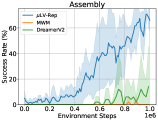
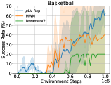
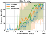
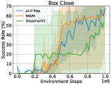
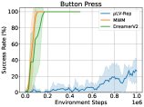
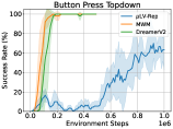
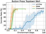
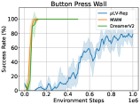
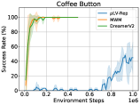
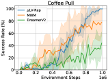
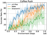
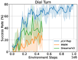
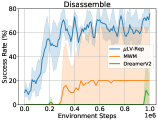
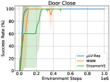
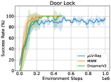
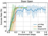
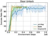
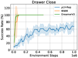
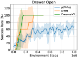
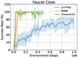
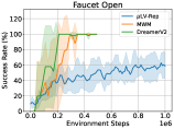
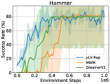
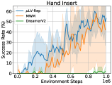
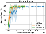
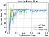
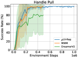
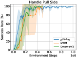
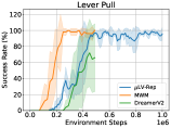
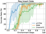
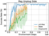
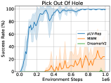
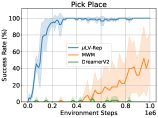
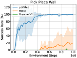
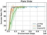
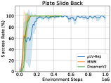
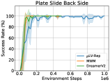
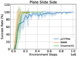
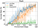
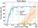
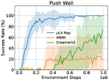
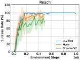
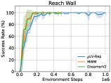
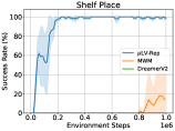
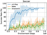
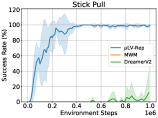
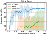
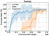
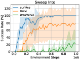
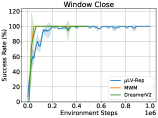
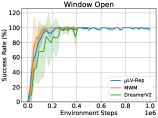
Figure 5: Overall performance on MetaWorld tasks.

In particular, we employ visual observations with dimensions of 64 × 64 × 3 and apply a variational autoencoder (VAE) to learn representations for these visual observations. The VAE is first pre-trained with random trajectories at the beginning and then fine-tuned during the online learning procedure. It produces compact vector representations for the images, which are then forwarded as input to our representation learning method. We apply actor-critic Learning based on the representation learned by VAE. The configuration of used tasks are given in Table 1. The hyperparameters used in the RL agent are shown in Table 2.

Table 1: Configuration of environments.

Hyperparameter	Value
Image observation	64$\times$64$\times 3$
Image normalization	Mean: $(0.485,0.456,0.406)$, Std: $(0.229,0.224,0.225)$
Action repeat	2
Episode length	500 (Meta-world), 1000 (DMC)
Normalize action	[-1,1]
Camera	corner2 (Meta-world), camera2 (DMC)
Total steps in environment	1M (Meta-world), 0.5M (DMC)

Table 2: Hyperparameters in $\mu$LV-Rep. The numbers in Conv and MLP denote the output channels and units.

Hyperparameter	Value
Buffer size	1,000,000
Batch size	256
Random steps	4000
Pretrain step	10000
Features dim.	100
Hidden dim.	1024
Encoder	(Conv(32), Conv(32), Conv(32), Conv(32), MLP(100))
Image Decoder	(MLP(100), MLP(1024), ConvT(32), ConvT(32), ConvT(32), ConvT(32), Conv(3))
Actor Network	(MLP(1024),MLP(1024),MLP(Action Space))
Critic Network	(MLP(1024),MLP(1024),MLP(1))
Optimizer	Adam
Learning rate	0.0001
Discount	0.99
Critic soft-update rate	0.01
Evaluate interval	10,000
Evaluate episodes	10 (Meta-world), 5 (DMC)

H.1 Ablation Studies

We perform ablation studies to demonstrate the effects of the major components, including representation dimension and window size, as illustrated below. Figure 6 presents an ablation study on representation dimension, where we compare $\mu$LV-Rep with latent representation dimensions 2048, 512, and 128. We also ablate the effect of window size $L$. In Figure 7, we compare $\mu$LV-Rep with window size $L=1,3,5$. We also compare DrQ-v2 [Yarats et al., 2022] with $L=1,3,5$ to show the effect of $L$ on other algorithms. The results show that for $L=1$, both $\mu$LV-Rep and DrQ-v2 struggle with learning, which confirms the Non-Markovian property of the DMC control problems. We can also find that $L=3$ is sufficient for learning in both test domains.

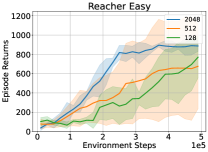
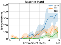
Figure 6: Ablation of feature dimension on visual control tasks from DeepMind Control Suites. Increasing the dimension of the feature gets better performance.

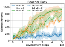
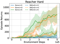
Figure 7: Ablation of window size $L$ on visual control tasks from DeepMind Control Suites. $L=3$ is sufficient for learning in both test domains.

H.2 Experiment of Partially Observable Continuous Control

We also evaluate the proposed approach on RL tasks with partial observations, constructed based on the OpenAI gym MuJoCo [Todorov et al., 2012]. Standard MuJoCo tasks from the OpenAI gym and DeepMind Control Suites are not partially observable. To generate partially observable problems based on these tasks, we adopt a widely employed approach of masking velocities within the observations [Ni et al., 2021, Weigand et al., 2021, Gangwani et al., 2020]. In this way, it becomes impossible to extract complete decision-making information from a single environment observation, yet the ability to reconstruct the missing observation remains achievable by aggregating past observations. We provide the best performance when using the original fully observable states (without velocity masking) as input, denoted by Best-FO (Best result with Full Observations). This gives a reference for the best result an algorithm is expected to achieve in our tests.

We consider four baselines in the experiments, including two model-based methods Dreamer [Hafner et al., 2020, 2021] and Stochastic Latent Actor-Critic (SLAC) [Lee et al., 2020], and a model-free baseline, SAC-MLP, that concatenates history sequences (past four observations) as input to an MLP layer for both the critic and policy. This simple baseline can be viewed as an analogue to how DQN processes observations in Atari games [Mnih et al., 2013] as a sanity check. We also compare to the neural PSR [Guo et al., 2018]. We compare all algorithms after running 200K environment steps. This setup exactly follows the benchmark [Wang et al., 2019], which has been widely adopted in [Zhang et al., 2022, Ren et al., 2023c, b] for fairness. All results are averaged across four random seeds. Table 3 presents all the experimental results, averaged over four random seeds. The results clearly demonstrate that the proposed method consistently delivers either competitive or superior outcomes across all domains compared to both the model-based and model-free baselines. We note that in most domains, $\mu$LV-Rep nearly matches the performance of Best-FO, further confirming that the proposed method is able to extract useful representations for decision-making in partially observable environments.

Table 3: Performance on various continuous control problems with partial observation. All results are averaged across 4 random seeds and a window size of 10K. $\mu$LV-Rep achieves the best performance compared to the baselines. Here, Best-FO denotes the performance of LV-Rep using full observations as inputs, providing a reference on how well an algorithm can achieve most in our tests.

	HalfCheetah	Humanoid	Walker	Ant	Hopper
$\mu$LV-Rep	3596.2 $\pm$ 874.5	806.7 $\pm$ 120.7	1298.1$\pm$ 276.3	1621.4 $\pm$ 472.3	1096.4 $\pm$ 130.4
Dreamer-v2	2863.8 $\pm$ 386	672.5 $\pm$ 36.6	1305.8 $\pm$ 234.2	1252.1 $\pm$ 284.2	758.3 $\pm$ 115.8
SAC-MLP	1612.0 $\pm$ 223	242.1 $\pm$ 43.6	736.5 $\pm$ 65.6	1612.0 $\pm$ 223	614.15 $\pm$ 67.6
SLAC	3012.4 $\pm$ 724.6	387.4 $\pm$ 69.2	536.5 $\pm$ 123.2	1134.8 $\pm$ 326.2	739.3 $\pm$ 98.2
PSR	2679.75$\pm$386	534.4 $\pm$ 36.6	862.4 $\pm$ 355.3	1128.3 $\pm$ 166.6	818.8 $\pm$ 87.2
Best-FO	5557.6$\pm$439.5	1086$\pm$278.2	2523.5$\pm$333.9	2511.8$\pm$460.0	2204.8$\pm$496.0
	Cheetah-run	Walker-run	Hopper-run	Humanoid-run	Pendulum
$\mu$LV-Rep	525.3 $\pm$ 89.2	702.3 $\pm$ 124.3	69.3$\pm$ 12.8	9.8 $\pm$ 6.4	168.2 $\pm$ 5.3
Dreamer-v2	602.3 $\pm$ 48.5	438.2 $\pm$ 78.2	59.2 $\pm$ 15.9	2.3 $\pm$ 0.4	172.3 $\pm$ 8.0
SAC-MLP	483.3 $\pm$ 77.2	279.8 $\pm$ 190.6	19.2 $\pm$ 2.3	1.2 $\pm$ 0.1	163.6 $\pm$ 9.3
SLAC	105.1 $\pm$ 30.1	139.2 $\pm$ 3.4	36.1 $\pm$ 15.3	0.9 $\pm$ 0.1	167.3 $\pm$ 11.2
PSR	173.7 $\pm$ 25.7	57.4 $\pm$ 7.4	23.2 $\pm$ 9.5	0.8 $\pm$ 0.1	159.4 $\pm$ 9.2
Best-FO	639.3$\pm$24.5	724.2$\pm$37.8	72.9$\pm$40.6	11.8$\pm$6.8	167.1$\pm$3.1

References

- Agarwal et al. (2020) Alekh Agarwal, Sham Kakade, Akshay Krishnamurthy, and Wen Sun. Flambe: Structural complexity and representation learning of low rank mdps. Advances in neural information processing systems, 33:20095–20107, 2020.
- Aronszajn (1950) Nachman Aronszajn. Theory of reproducing kernels. Transactions of the American mathematical society, 68(3):337–404, 1950.
- Åström (1965) Karl Johan Åström. Optimal control of markov processes with incomplete state information. Journal of mathematical analysis and applications, 10(1):174–205, 1965.
- Azizzadenesheli et al. (2016) Kamyar Azizzadenesheli, Alessandro Lazaric, and Animashree Anandkumar. Reinforcement learning of pomdps using spectral methods. In COLT, 2016.
- Bakker (2001) Bram Bakker. Reinforcement learning with long short-term memory. NeurIPS, 2001.
- Barreto et al. (2017) André Barreto, Will Dabney, Rémi Munos, Jonathan J Hunt, Tom Schaul, Hado P van Hasselt, and David Silver. Successor features for transfer in reinforcement learning. NeurIPS, 2017.
- Barth-Maron et al. (2018) Gabriel Barth-Maron, Matthew W Hoffman, David Budden, Will Dabney, Dan Horgan, Dhruva Tb, Alistair Muldal, Nicolas Heess, and Timothy Lillicrap. Distributed distributional deterministic policy gradients. arXiv preprint arXiv:1804.08617, 2018.
- Berner et al. (2019) Christopher Berner, Greg Brockman, Brooke Chan, Vicki Cheung, Przemysław Dębiak, Christy Dennison, David Farhi, Quirin Fischer, Shariq Hashme, Chris Hesse, et al. Dota 2 with large scale deep reinforcement learning. arXiv preprint arXiv:1912.06680, 2019.
- Chen et al. (2016) Min Chen, Emilio Frazzoli, David Hsu, and Wee Sun Lee. Pomdp-lite for robust robot planning under uncertainty. In 2016 IEEE International Conference on Robotics and Automation (ICRA), pages 5427–5433. IEEE, 2016.
- Dayan (1993) Peter Dayan. Improving generalization for temporal difference learning: The successor representation. Neural computation, 5(4):613–624, 1993.
- Deisenroth and Peters (2012) Marc Peter Deisenroth and Jan Peters. Solving nonlinear continuous state-action-observation pomdps for mechanical systems with gaussian noise. In European Workshop on Reinforcement Learning, 2012.
- Du et al. (2019) Simon Du, Akshay Krishnamurthy, Nan Jiang, Alekh Agarwal, Miroslav Dudik, and John Langford. Provably efficient rl with rich observations via latent state decoding. In International Conference on Machine Learning, pages 1665–1674. PMLR, 2019.
- Duan et al. (2019) Yaqi Duan, Tracy Ke, and Mengdi Wang. State aggregation learning from markov transition data. NeurIPS, 2019.
- Efroni et al. (2022) Yonathan Efroni, Chi Jin, Akshay Krishnamurthy, and Sobhan Miryoosefi. Provable reinforcement learning with a short-term memory. In International Conference on Machine Learning, pages 5832–5850. PMLR, 2022.
- Even-Dar et al. (2007) Eyal Even-Dar, Sham M Kakade, and Yishay Mansour. The value of observation for monitoring dynamic systems. In IJCAI, pages 2474–2479, 2007.
- Ferns et al. (2004) Norm Ferns, Prakash Panangaden, and Doina Precup. Metrics for finite markov decision processes. In UAI, 2004.
- Gangwani et al. (2020) Tanmay Gangwani, Joel Lehman, Qiang Liu, and Jian Peng. Learning belief representations for imitation learning in pomdps. In UAI, 2020.
- Gelada et al. (2019) Carles Gelada, Saurabh Kumar, Jacob Buckman, Ofir Nachum, and Marc G Bellemare. Deepmdp: Learning continuous latent space models for representation learning. In ICML, 2019.
- Golowich et al. (2022) Noah Golowich, Ankur Moitra, and Dhruv Rohatgi. Learning in observable pomdps, without computationally intractable oracles. Advances in Neural Information Processing Systems, 35:1458–1473, 2022.
- Gregor et al. (2019) Karol Gregor, Danilo Jimenez Rezende, Frederic Besse, Yan Wu, Hamza Merzic, and Aaron van den Oord. Shaping belief states with generative environment models for rl. NeurIPS, 2019.
- Guo et al. (2023) Jiacheng Guo, Zihao Li, Huazheng Wang, Mengdi Wang, Zhuoran Yang, and Xuezhou Zhang. Provably efficient representation learning with tractable planning in low-rank pomdp. arXiv preprint arXiv:2306.12356, 2023.
- Guo et al. (2016) Zhaohan Daniel Guo, Shayan Doroudi, and Emma Brunskill. A pac rl algorithm for episodic pomdps. In Artificial Intelligence and Statistics, pages 510–518. PMLR, 2016.
- Guo et al. (2018) Zhaohan Daniel Guo, Mohammad Gheshlaghi Azar, Bilal Piot, Bernardo A Pires, and Rémi Munos. Neural predictive belief representations. arXiv preprint arXiv:1811.06407, 2018.
- Haarnoja et al. (2018) Tuomas Haarnoja, Aurick Zhou, Pieter Abbeel, and Sergey Levine. Soft actor-critic: Off-policy maximum entropy deep reinforcement learning with a stochastic actor. In International conference on machine learning, pages 1861–1870. PMLR, 2018.
- Hafner et al. (2020) Danijar Hafner, Timothy Lillicrap, Jimmy Ba, and Mohammad Norouzi. Dream to control: Learning behaviors by latent imagination. In International Conference on Learning Representations, 2020. URL https://openreview.net/forum?id=S1lOTC4tDS.
- Hafner et al. (2021) Danijar Hafner, Timothy P Lillicrap, Mohammad Norouzi, and Jimmy Ba. Mastering atari with discrete world models. In International Conference on Learning Representations, 2021. URL https://openreview.net/forum?id=0oabwyZbOu.
- Hausknecht and Stone (2015) Matthew Hausknecht and Peter Stone. Deep recurrent q-learning for partially observable mdps. In AAAI fall symposium series, 2015.
- Hauskrecht and Fraser (2000) Milos Hauskrecht and Hamish Fraser. Planning treatment of ischemic heart disease with partially observable markov decision processes. Artificial intelligence in medicine, 18(3):221–244, 2000.
- Heess et al. (2015) Nicolas Heess, Jonathan J Hunt, Timothy P Lillicrap, and David Silver. Memory-based control with recurrent neural networks. arXiv:1512.04455, 2015.
- Huang et al. (2023) Ruiquan Huang, Yingbin Liang, and Jing Yang. Provably efficient ucb-type algorithms for learning predictive state representations. arXiv preprint arXiv:2307.00405, 2023.
- Igl et al. (2018) Maximilian Igl, Luisa Zintgraf, Tuan Anh Le, Frank Wood, and Shimon Whiteson. Deep variational reinforcement learning for pomdps. In ICML, 2018.
- Jiang et al. (2021) Haoming Jiang, Bo Dai, Mengjiao Yang, Tuo Zhao, and Wei Wei. Towards automatic evaluation of dialog systems: A model-free off-policy evaluation approach. arXiv preprint arXiv:2102.10242, 2021.
- Jin et al. (2020a) Chi Jin, Sham Kakade, Akshay Krishnamurthy, and Qinghua Liu. Sample-efficient reinforcement learning of undercomplete pomdps. Advances in Neural Information Processing Systems, 33:18530–18539, 2020a.
- Jin et al. (2020b) Chi Jin, Zhuoran Yang, Zhaoran Wang, and Michael I Jordan. Provably efficient reinforcement learning with linear function approximation. In COLT, 2020b.
- Kaelbling et al. (1998) Leslie Pack Kaelbling, Michael L Littman, and Anthony R Cassandra. Planning and acting in partially observable stochastic domains. Artificial intelligence, 101(1-2):99–134, 1998.
- Kaufmann et al. (2023) Elia Kaufmann, Leonard Bauersfeld, Antonio Loquercio, Matthias Müller, Vladlen Koltun, and Davide Scaramuzza. Champion-level drone racing using deep reinforcement learning. Nature, 620(7976):982–987, 2023.
- Kingma and Welling (2013) Diederik P Kingma and Max Welling. Auto-encoding variational bayes. arXiv preprint arXiv:1312.6114, 2013.
- Kulkarni et al. (2016) Tejas D Kulkarni, Ardavan Saeedi, Simanta Gautam, and Samuel J Gershman. Deep successor reinforcement learning. arXiv:1606.02396, 2016.
- Lee et al. (2020) Alex X Lee, Anusha Nagabandi, Pieter Abbeel, and Sergey Levine. Stochastic latent actor-critic: Deep reinforcement learning with a latent variable model. NeurIPS, 2020.
- Levine et al. (2016) Sergey Levine, Chelsea Finn, Trevor Darrell, and Pieter Abbeel. End-to-end training of deep visuomotor policies. The Journal of Machine Learning Research, 17(1):1334–1373, 2016.
- Littman and Sutton (2001) Michael Littman and Richard S Sutton. Predictive representations of state. Advances in neural information processing systems, 14, 2001.
- Liu et al. (2022) Qinghua Liu, Alan Chung, Csaba Szepesvári, and Chi Jin. When is partially observable reinforcement learning not scary? In Conference on Learning Theory, pages 5175–5220. PMLR, 2022.
- Liu et al. (2023) Qinghua Liu, Praneeth Netrapalli, Csaba Szepesvari, and Chi Jin. Optimistic mle: A generic model-based algorithm for partially observable sequential decision making. In Proceedings of the 55th Annual ACM Symposium on Theory of Computing, pages 363–376, 2023.
- Mahadevan and Maggioni (2007) Sridhar Mahadevan and Mauro Maggioni. Proto-value functions: A laplacian framework for learning representation and control in markov decision processes. JMLR, 8(10), 2007.
- Meng et al. (2021) Lingheng Meng, Rob Gorbet, and Dana Kulić. Memory-based deep reinforcement learning for pomdps. In 2021 IEEE/RSJ International Conference on Intelligent Robots and Systems (IROS), pages 5619–5626. IEEE, 2021.
- Mnih et al. (2013) Volodymyr Mnih, Koray Kavukcuoglu, David Silver, Alex Graves, Ioannis Antonoglou, Daan Wierstra, and Martin Riedmiller. Playing atari with deep reinforcement learning. arXiv preprint arXiv:1312.5602, 2013.
- Munos and Szepesvári (2008) Rémi Munos and Csaba Szepesvári. Finite-time bounds for fitted value iteration. Journal of Machine Learning Research, 9(5), 2008.
- Nachum and Dai (2020) Ofir Nachum and Bo Dai. Reinforcement learning via fenchel-rockafellar duality. arXiv preprint arXiv:2001.01866, 2020.
- Nachum and Yang (2021) Ofir Nachum and Mengjiao Yang. Provable representation learning for imitation with contrastive fourier features. NeurIPS, 2021.
- Ni et al. (2021) Tianwei Ni, Benjamin Eysenbach, and Ruslan Salakhutdinov. Recurrent model-free rl is a strong baseline for many pomdps. arXiv:2110.05038, 2021.
- Oord et al. (2018) Aaron van den Oord, Yazhe Li, and Oriol Vinyals. Representation learning with contrastive predictive coding. arXiv:1807.03748, 2018.
- Papadimitriou and Tsitsiklis (1987) Christos H Papadimitriou and John N Tsitsiklis. The complexity of markov decision processes. Mathematics of operations research, 12(3):441–450, 1987.
- Paulsen and Raghupathi (2016) Vern I Paulsen and Mrinal Raghupathi. An introduction to the theory of reproducing kernel Hilbert spaces, volume 152. Cambridge university press, 2016.
- Puterman (2014) Martin L Puterman. Markov decision processes: discrete stochastic dynamic programming. John Wiley & Sons, 2014.
- Ren et al. (2022) Tongzheng Ren, Tianjun Zhang, Csaba Szepesvári, and Bo Dai. A free lunch from the noise: Provable and practical exploration for representation learning. In Uncertainty in Artificial Intelligence, pages 1686–1696. PMLR, 2022.
- Ren et al. (2023a) Tongzheng Ren, Zhaolin Ren, Na Li, and Bo Dai. Stochastic nonlinear control via finite-dimensional spectral dynamic embedding. arXiv preprint arXiv:2304.03907, 2023a.
- Ren et al. (2023b) Tongzheng Ren, Chenjun Xiao, Tianjun Zhang, Na Li, Zhaoran Wang, Sujay Sanghavi, Dale Schuurmans, and Bo Dai. Latent variable representation for reinforcement learning. In The Eleventh International Conference on Learning Representations, 2023b.
- Ren et al. (2023c) Tongzheng Ren, Tianjun Zhang, Lisa Lee, Joseph E Gonzalez, Dale Schuurmans, and Bo Dai. Spectral decomposition representation for reinforcement learning. ICLR, 2023c.
- Riesz and Nagy (2012) Frigyes Riesz and Béla Sz Nagy. Functional analysis. Courier Corporation, 2012.
- Ross et al. (2008) Stéphane Ross, Joelle Pineau, Sébastien Paquet, and Brahim Chaib-Draa. Online planning algorithms for pomdps. Journal of Artificial Intelligence Research, 32:663–704, 2008.
- Roy and Gordon (2002) Nicholas Roy and Geoffrey J Gordon. Exponential family pca for belief compression in pomdps. Advances in Neural Information Processing Systems, 15, 2002.
- Schmidhuber (1990) Jürgen Schmidhuber. Reinforcement learning in markovian and non-markovian environments. NeurIPS, 3, 1990.
- Seo et al. (2023) Younggyo Seo, Danijar Hafner, Hao Liu, Fangchen Liu, Stephen James, Kimin Lee, and Pieter Abbeel. Masked world models for visual control. In Conference on Robot Learning, pages 1332–1344. PMLR, 2023.
- Simchowitz et al. (2021) Max Simchowitz, Christopher Tosh, Akshay Krishnamurthy, Daniel J Hsu, Thodoris Lykouris, Miro Dudik, and Robert E Schapire. Bayesian decision-making under misspecified priors with applications to meta-learning. Advances in Neural Information Processing Systems, 34:26382–26394, 2021.
- Smallwood and Sondik (1973) Richard D Smallwood and Edward J Sondik. The optimal control of partially observable markov processes over a finite horizon. Operations research, 21(5):1071–1088, 1973.
- Steinwart and Scovel (2012) Ingo Steinwart and Clint Scovel. Mercer’s theorem on general domains: On the interaction between measures, kernels, and rkhss. Constructive Approximation, 35(3):363–417, 2012.
- Tassa et al. (2018) Yuval Tassa, Yotam Doron, Alistair Muldal, Tom Erez, Yazhe Li, Diego de Las Casas, David Budden, Abbas Abdolmaleki, Josh Merel, Andrew Lefrancq, et al. Deepmind control suite. arXiv preprint arXiv:1801.00690, 2018.
- Todorov et al. (2012) Emanuel Todorov, Tom Erez, and Yuval Tassa. Mujoco: A physics engine for model-based control. In 2012 IEEE/RSJ international conference on intelligent robots and systems, pages 5026–5033. IEEE, 2012.
- Uehara et al. (2021) Masatoshi Uehara, Xuezhou Zhang, and Wen Sun. Representation learning for online and offline rl in low-rank mdps. arXiv preprint arXiv:2110.04652, 2021.
- Uehara et al. (2022) Masatoshi Uehara, Ayush Sekhari, Jason D Lee, Nathan Kallus, and Wen Sun. Provably efficient reinforcement learning in partially observable dynamical systems. Advances in Neural Information Processing Systems, 35:578–592, 2022.
- Wang et al. (2019) Tingwu Wang, Xuchan Bao, Ignasi Clavera, Jerrick Hoang, Yeming Wen, Eric Langlois, Shunshi Zhang, Guodong Zhang, Pieter Abbeel, and Jimmy Ba. Benchmarking model-based reinforcement learning. arXiv preprint arXiv:1907.02057, 2019.
- Weigand et al. (2021) Stephan Weigand, Pascal Klink, Jan Peters, and Joni Pajarinen. Reinforcement learning using guided observability. arXiv:2104.10986, 2021.
- Wierstra et al. (2007) Daan Wierstra, Alexander Foerster, Jan Peters, and Juergen Schmidhuber. Solving deep memory pomdps with recurrent policy gradients. In ICANN, 2007.
- Wu et al. (2018) Yifan Wu, George Tucker, and Ofir Nachum. The laplacian in rl: Learning representations with efficient approximations. arXiv:1810.04586, 2018.
- Yang and Wang (2020) Lin Yang and Mengdi Wang. Reinforcement learning in feature space: Matrix bandit, kernels, and regret bound. In International Conference on Machine Learning, pages 10746–10756. PMLR, 2020.
- Yang et al. (2021) Mengjiao Yang, Sergey Levine, and Ofir Nachum. Trail: Near-optimal imitation learning with suboptimal data. arXiv:2110.14770, 2021.
- Yarats et al. (2020) Denis Yarats, Ilya Kostrikov, and Rob Fergus. Image augmentation is all you need: Regularizing deep reinforcement learning from pixels. In International conference on learning representations, 2020.
- Yarats et al. (2021) Denis Yarats, Amy Zhang, Ilya Kostrikov, Brandon Amos, Joelle Pineau, and Rob Fergus. Improving sample efficiency in model-free reinforcement learning from images. In Proceedings of the AAAI Conference on Artificial Intelligence, volume 35, pages 10674–10681, 2021.
- Yarats et al. (2022) Denis Yarats, Rob Fergus, Alessandro Lazaric, and Lerrel Pinto. Mastering visual continuous control: Improved data-augmented reinforcement learning. In International Conference on Learning Representations, 2022.
- Yu et al. (2019) Tianhe Yu, Deirdre Quillen, Zhanpeng He, Ryan Julian, Karol Hausman, Chelsea Finn, and Sergey Levine. Meta-world: A benchmark and evaluation for multi-task and meta reinforcement learning. In Conference on Robot Learning (CoRL), 2019. URL https://arxiv.org/abs/1910.10897.
- Zhan et al. (2022) Wenhao Zhan, Masatoshi Uehara, Wen Sun, and Jason D Lee. Pac reinforcement learning for predictive state representations. arXiv preprint arXiv:2207.05738, 2022.
- Zhang et al. (2020) Amy Zhang, Rowan McAllister, Roberto Calandra, Yarin Gal, and Sergey Levine. Learning invariant representations for reinforcement learning without reconstruction. arXiv:2006.10742, 2020.
- Zhang et al. (2019) Marvin Zhang, Sharad Vikram, Laura Smith, Pieter Abbeel, Matthew Johnson, and Sergey Levine. Solar: Deep structured representations for model-based reinforcement learning. In ICML, 2019.
- Zhang et al. (2022) Tianjun Zhang, Tongzheng Ren, Mengjiao Yang, Joseph Gonzalez, Dale Schuurmans, and Bo Dai. Making linear mdps practical via contrastive representation learning. In ICML, 2022.
- Zhang et al. (2023) Tianjun Zhang, Tongzheng Ren, Chenjun Xiao, Wenli Xiao, Joseph Gonzalez, Dale Schuurmans, and Bo Dai. Energy-based predictive representations for partially observed reinforcement learning. In The 39th Conference on Uncertainty in Artificial Intelligence, 2023. URL https://openreview.net/forum?id=Z1BobPmCTy.
- Zhu et al. (2017) Pengfei Zhu, Xin Li, Pascal Poupart, and Guanghui Miao. On improving deep reinforcement learning for pomdps. arXiv preprint arXiv:1704.07978, 2017.