Day-Ahead Programming of Energy Communities Participating in Pay-as-Bid Service Markets

Abstract

This paper proposes an optimal strategy for a Renewable Energy Community participating in the Italian pay-as-bid ancillary service market. The community is composed by a group of residential customers sharing a common facility equipped with a PV power plant and a battery energy storage system. This battery is employed to maximize the community cash flow obtained by the participation in the service market. A scenario-based optimization problem is defined to size the bids to be submitted to the market and to define the corresponding optimal battery energy exchange profile for the day ahead. The proposed optimization scheme is able to take in to account the probability of acceptance of the service market bids and the uncertainties on the forecasts of PV generation and energy demands. Results prove the effectiveness of the approach and the economic advantages on participating in the service market.

I Introduction

Among the solutions proposed to integrate Renewable Energy Sources in the power system, Renewable Energy Communities, defined by the EU directive [1], have emerged as a dynamic and multifaceted entity composed by residential customers, small-medium enterprises and/or local authorities, engaging in various activities centered on the ownership and management of RESs. The primary aim of RECs is to generate, store, and sell renewable energy by facilitating the exchange of this energy among its members.

In the Italian law transportation [2] of the EU directive, RECs’ members are encouraged to share renewable energy through the payment of an incentive, but they also have the opportunity to be a player in the Ancillary Service Market (ACS), which follows a pay-as-bid mechanism. In literature, different techniques are proposed to manage RES generation and storage systems to optimize their functioning in the context of RECs compliant with the Italian law such as [3, 4, 5]. Few works optimize RECs for multi-market participation. A bidding-based peer-to-peer energy transaction optimization model is presented in [6]. The proposed model considers REC members willingness to pay for green energy and minimizes the community operating costs. A two-stage stochastic programming model for energy trading, evaluating the potential to supply ancillary services is presented in [7]. However, in literature there is a lack of papers addressing the problem of REC optimal participation in pay-as-bid service markets.

In this paper we provide an optimal scenario-based day-ahead programming algorithm that optimizes the participation of REC in the Italian ACS. As shown in Figure  1, the REC is composed by a group of residential customers sharing a Community Facility (CF) equipped with a Photovoltaic (PV) power plant, a Battery Energy Storage System (BESS) and an internal load. The proposed algorithm allows the REC to optimally size the bids to be submitted to the ACS and to define the BESS energy exchange for the day ahead, taking into account the uncertainties on the forecasts of PV generation and energy demands, as well as the probability of acceptance of the ACS bids. Simulation results that prove the effectiveness of the approach and the potential economic advantages for a REC in participating in the ACS.

II System Architecture and Market Rules

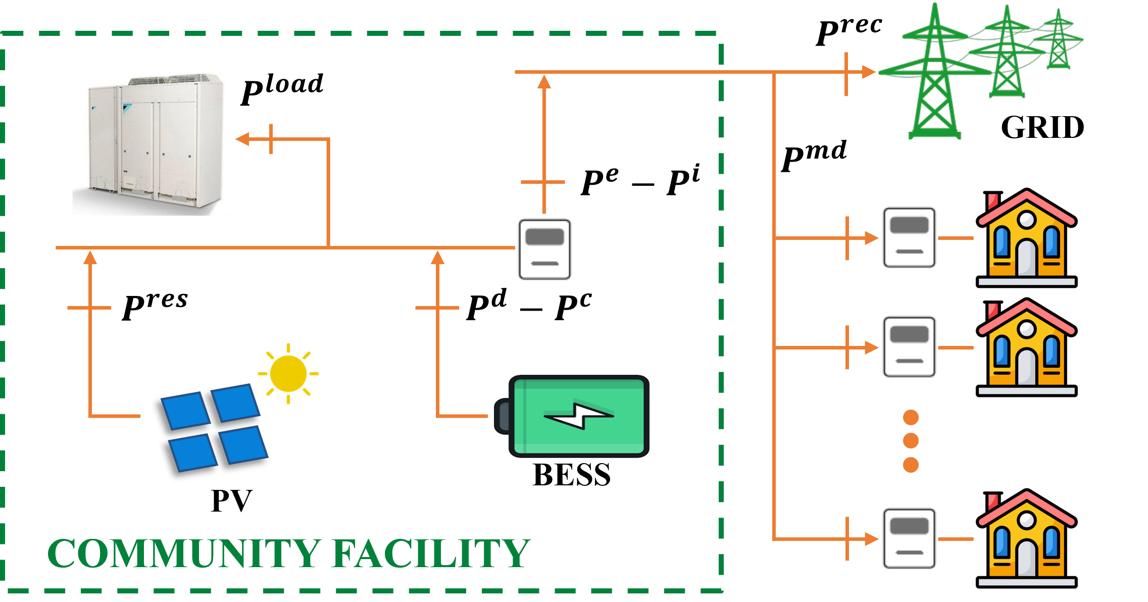
Figure 1: REC architecture.

The schematic architecture of the considered REC is shown in Figure 1. Here, links do not necessarily compose an actual electrical network since, according to the Italian law [2], the energy exchange within a REC can be virtual, with the unique condition that RESs and consumers are connected under the same HV/MV substation.

II-A Energy Markets Rules

During any hour $k=1,2,\ldots,24$, the CF can export energy $P^{e}_{k}$ or import energy $P^{i}_{k}$ with the utility grid in order to meet its internal demand $P^{load}_{k}$ and share energy with the REC members. According to the Italian law [2], the CF does not have to fully meet the aggregated members demand $P^{md}_{k}$, as every member keep their independence and contract with their energy provider. As a virtual entity, the REC energy exchange with the utility grid is

$$P^{rec}_{k}=P^{e}_{k}-P^{i}_{k}-P^{md}_{k}$$ (1)

with positive values meaning export.

The REC pays $c^{i}_{k}$ for the energy imported by the CF from the utility grid and is paid $c^{e}_{k}$ for the energy exported by the CF to the utility grid. According to the Italian law [2], the REC gets an incentive $\gamma^{sh}$ proportional to the shared energy $P^{sh}$, defined as the minimum between the aggregated members energy demand and the exported renewable energy, i.e.

$$P^{sh}_{k}=\min\{P^{e}_{k},P^{md}_{k}\}.$$ (2)

In this paper we consider the participation of the REC in the Italin acmsd where the Transmission System Operator (TSO) acts as the central counterpart. When necessary, the TSO requires participants to modify their baseline, declared the day before, by generate or consume more/less power. In the ACS market sessions, participants declare the action that they are willing to realize and submit their prices for that. The TSO accept bids according to a pay-as-bid mechanism.

More specifically, REC’s bid in the ACS, when accepted, is acknowledged by an economic reward i.e., the REC is willing to modify its baseline and it is paid to generate more (or consume less) energy (sell bid) or, on the contrary, pays to generate less (or consume more) energy (purchase bid). Bids are composed by a couple price-energy variation, $(c^{+}_{k},P^{+}_{k})$ for sell bids and $(c^{-}_{k},P^{-}_{k})$ for purchase bids. Service variations $P^{+}_{k}$ and $P^{-}_{k}$ are defied with respect a baseline $\hat{P}_{k}^{rec}$ that the REC must declare together with the bids.

We assume that the TSO is price-taker with respect to the REC. This means that a sell bid is fully accepted when the offered price $c^{+}_{k}$ is lower than the maximum accepted sell price in the ACS $\overline{c}^{+}_{k}$, while a purchase bid is fully accepted when the offered price $c^{-}$ is higher than the minimum accepted purchase price in the ACS $\underline{c}^{-}_{k}$. Clearly, $\overline{c}^{+}_{k}$ is usually higher than $c^{e}$, as well as, $\underline{c}^{-}_{k}$ is usually lower than $c^{i}_{k}$.

Therefore, if at any hour $k$ a sell bid is accepted the REC must exchange with the grid the energy $\hat{P}_{k}^{rec}+P^{+}_{k}$. In the case that $P^{rec}_{k}<\hat{P}_{k}^{rec}+P^{+}$, the error $E^{+}_{k}=\hat{P}_{k}^{rec}+P^{+}_{k}-P^{rec}_{k}$ is paid by the REC to the TSO with a penalty $p^{+}$ higher than $\overline{c}^{+}_{k}$. Similarly, if a purchase bid is accepted the REC energy exchange with the grid should be $\hat{P}_{k}^{rec}-P^{-}_{k}$ and in the case that $P^{rec}_{k}>\hat{P}_{k}^{rec}-P^{-}_{k}$, the service error $E^{-}_{k}=P^{rec}_{k}-(\hat{P}_{k}^{rec}-P^{-}_{k})$ is paid by the TSO to the REC with a price $p^{-}$ lower than $\underline{c}^{-}_{k}$.

II-B Objective

The objective of this paper is to program, for all hours $k=1,2,\ldots,24$ of the day- ahead, the REC baseline $\hat{P}^{rec}_{k}$ and the sell and buy bids to be submitted to the ACS, $(c^{+}_{k},P^{+}_{k})$ and $(c^{-}_{k},P^{-}_{k})$ assuming to be able to control the community BESS power exchange and being provided with: 1) initial State of Charge (SoC) of the BESS $S_{0}$; 2) forecasts the market prices $c^{e}_{k}$, $c^{i}_{k}$, $\overline{c}^{+}_{k}$ and $\underline{c}^{-}_{k}$; 3) forecasts of renewable generation and demands, $P^{res}_{k}$, $P^{load}_{l}$ and $P^{md}_{k}$.

The program objective is to maximize the day cash flow of the community. When the day-ahead optimization is processed, this cash flow is a random variable since we are provided with forecasts of prices, generation and demands. Therefore, we actually realize stochastic optimization where the expected value of the day cash flow is maximized.

III Forecasting Methods

III-A Energy Prices Forecast

We first suppose that, when the day-ahead programming is computed, import and export prices $c^{i}_{k}$ and $c^{e}_{k}$ with $k=1,2,\ldots,24$ are known. Differently, ACS prices cannot be known a-priori. Therefore, a scenario based forecast approach is adopted. Hystorical data of the maximum accepted sell prices $\overline{c}^{+}_{k}$ and minimum accepted purchase prices $\underline{c}^{-}_{k}$ (available on the Italian electricity market operator web repository [8]) are collected by considering each couple of daily trajectories of $\overline{c}^{+}_{k}$ and $\underline{c}^{-}_{k}$ as one scenario. Then, using the scenario reduction algorithm in [9] a reduced set of $n_{m}$ scenarios $\{\{\overline{c}^{+}_{k,s}\}_{k=1}^{24},\{\underline{c}^{-}_{k,s}\}_{k=1}^{24}\}_{s=1}^{n_{m}}$ is obtained, each associated to the probability $\pi^{m}_{s}$, with $s=1,\ldots,n_{m}$.

III-B Demands and RES Generation Forecasts

In [10], a methodology is proposed to model time series with a Discrete Markov Chain (DMC) through an adaptive online algorithm with minimal computational efforts. The constructed DMC can then be used to sample possible future scenarios given the current actual state of the DMC. The algorithm for the case of three variables i.e., RES generation $P^{res}$ and energy demands $P^{md}$ and $P^{load}$ is detailed in [3]. The DMC is used to generate 300 scenarios with a time length of 24 hours. Then, the scenario reduction algorithm in [9] is used to reduce the number of scenarios to $n_{r}$, each one with its own associated probability. The results are the forecast scenarios $\{\{P^{res}_{k,l}\}_{k=1}^{24},\{P^{load}_{k,l}\}_{k=1}^{24},\{P^{md}_{k,l}\}_{k=1}^{24}\}_{l=1}^{n_{r}}$, associated to the probability $\pi^{r}_{l}$, with $l=1,\ldots,n_{r}$.

IV Day-Ahead Programming

As stated in Section II-B, our objective is establish a day-ahead program for the CF with the objective of maximizing the expected value of the community cash flow. Since random time-series are involved, we formulate a stochastic optimization problem. Our choice is to carry out a scenario based optimization [11], where random time-series distributions are approximated by a set of scenario trajectories, each associated to an occurrence probability. As detailed in Section III-A and Section III-B the forecasts of all random time-series involved in our problem are built as scenarios. We have $n_{m}$ prices scenarios, indexed by $s=1,2,\ldots,n_{m}$ (Section III-A), and $n_{r}$ energy scenarios (for PV generation and demands, Section III-B), indexed by $l=1,2,\ldots,n_{r}$. In the following, if the value of a given variable $x_{k}$ depends on the realizations of the prices or the energy scenarios, we will indicate the corresponding realization of $x_{k}$ with $x_{k,s}$ or with $x_{k,l}$. In the case $x_{k}$ depends on both the scenarios’ realizations, the corresponding realization of $x_{k}$ will be indicated with $x_{k,s,l}$.

In order to define the day-ahead optimization problem we need to define a proper objective function and introduce a set of auxiliary variables and mixed-integer constraints modeling the ACS mechanism and the desired behaviour of the REC.

First of all we introduce two binary variables $b_{k}^{+/-}$ equal to 1 if the REC decides to submit a sell or a purchase bid at time $k$, respectively. Therefore:

$$0\leq P^{+}_{k}\leq P^{e}_{max} b^{+}_{k},\quad\ 0\leq P^{-}_{k}\leq P^{i}_{max}b^{-}_{k}$$ (3)

$$b^{+}_{k}+b^{-}_{k}\leq 1$$ (4)

where $P_{max}^{e}$ and $P_{max}^{i}$ are the maximum powers that CF can export to and import from the grid, respectively. Constraint (4) is introduced to impose that at a given time $k$ there be only one bid, either to sell or to purchase.

Let us now define two random variables $\Gamma_{k,s}^{+}$ and $\Gamma_{k,s}^{-}$ as the upward and downward variations that the REC must realize if the sell and purchase bids at time $k$ are accepted in the prices scenario $s$. Thus, according to the rules introduced in Section II-A, for all $s=1,2,\ldots,n_{m}$,

$$\Gamma^{+}_{k,s}=\delta^{+}_{k,s}{P}^{+}_{k}$$ (5)

$$\delta^{+}_{k,s}=1\Leftrightarrow c^{+}_{k}\leq\overline{c}^{+}_{k,s}$$ (6)

$$\Gamma^{-}_{k,s}=\delta^{-}_{k,s}{P}^{-}_{k}$$ (7)

$$\delta^{-}_{k,s}=1\Leftrightarrow c^{-}_{k}\geq\underline{c}^{-}_{k,s}$$ (8)

where $\delta^{+/-}_{k,s}$ are binary variables equal to one if, in the prices scenario $s$, sell or purchase bids are accepted.

Let us consider now the energy exchange of the CF and of the overall REC. If a sell (or purchase) bid is accepted, the upward (or downward) energy variation should be realized by the CF by using the energy reserve kept by the BESS. Moreover, we assume to use the BESS also to compensate the forecasting errors on PV generation and demands. This means that the energy exchanges of REC and CF will depend both on the prices and energy scenarios, meaning that $P^{rec}_{k}$, $P^{i}_{k}$ and $P^{e}_{k}$ become $P^{rec}_{k,s,l}$, $P^{i}_{k,s,l}$ and $P^{e}_{k,s,l}$. Under these assumptions, the CF energy balance is modeled by:

$$P^{e}_{k,s,l}-P^{i}_{k,s,l}=P^{res}_{k,l}-P^{load}_{k,l}+P^{d}_{k,s,l}-P^{c}_{k,s,l}$$ (9)

$$0\leq{P}^{e}_{k,s,l}\leq{\delta}^{e}_{k,s,l}P^{e}_{max}$$ (10)

$$0\leq{P}^{i}_{k,s,l}\leq(1-{\delta}^{e}_{k,s,l})P^{i}_{max}$$ (11)

where $\delta^{e}_{k,s,l}$ are binary variable equal to 1 if the CF is exporting energy. Moreover, the REC energy exchange (1) is represented as follows:

$$P^{rec}_{k,s,l}=P^{e}_{k,s,l}-P^{i}_{k,s,l}-P^{md}_{k,l}$$ (12)

$$\begin{aligned} &P^{rec}_{k,s,l}=\hat{P}^{rec}_{k}+w^{+}_{k,s,l}-w^{+}_{k,s,l}\\ &\qquad\qquad+\Gamma^{+}_{k,s}-E^{+}_{k,s,l}-(\Gamma^{-}_{k,s}-E^{-}_{k,s,l})\end{aligned}$$ (13)

$$0\leq E^{+}_{k,s,l}\leq\Gamma^{+}_{k,s,l},\quad 0\leq E^{-}_{k,s,l}\leq\Gamma^{-}_{k,s,l}$$ (14)

In (13) we impose the desired energy balance of the REC for all possible scenarios, i.e. variation from the baseline $\hat{P}^{rec}_{k}$ when one sell or purchase bid is submitted and accepted. $E^{+/-}_{k,s,l}$ can be considered as constraint relaxing variables, recalling that, if different from zero, the REC will pay penalties. While, $w_{k,s,l}^{+/-}$ are relaxing variable allowing the baseline to be modified according to the random variations of generation and demands in the scenarios where no bid is accepted.

We need now to impose that when bids are accepted, the service variations are realized by the CF using the BESS. Therefore, the following constraints must hold true:

$$\begin{aligned} &P^{e}_{k,s,l}-P^{i}_{k,s,l}=\hat{P}^{i}_{k,s,l}-\hat{P}^{e}_{k,s,l}\\ &\qquad\qquad\qquad\quad+\Gamma^{+}_{k,s}-E^{+}_{k,s,l}-(\Gamma^{-}_{k,s}-E^{-}_{k,s,l})\end{aligned}$$ (15)

$$0\leq\hat{P}^{e}_{k,s,l}\leq\hat{\delta}^{e}_{k,s,l}P^{e}_{max}$$ (16)

$$0\leq\hat{P}^{i}_{k,s,l}\leq(1-\hat{\delta}^{e}_{k,s,l})P^{i}_{max}$$ (17)

$$P^{d}_{k,s,l}-P^{c}_{k,s,l}=\hat{P}^{b}_{k}+\Gamma^{+}_{k,s,l}-\Gamma^{-}_{k,s,l}+v^{+}_{k,s,l}-v^{-}_{k,s,l}$$ (18)

$$0\leq{P}^{c}_{k,s,l}\leq P^{b}_{nom}{\delta}^{c}_{k,s,l}$$ (19)

$$0\leq{P}^{d}_{k,s,l}\leq P^{b}_{nom}(1-{\delta}^{c}_{k,s,l})$$ (20)

where $\hat{P}^{i}_{k,s,l}-\hat{P}^{e}_{k,s,l}$ is the CF baseline called to realize the REC baseline $\hat{P}^{rec}_{k}+w^{+}_{k,s,l}-w^{-}_{k,s,l}$ in (13) when no bid is accepted. Constraint (18) imposes that the service variations are effectively provided by the BESS. Here, $\hat{P}^{b}_{k}$ is the BESS baseline, followed by the BESS when no bid is accepted, whereas $v_{k,s,l}^{+/-}$ are relaxing variables which allow the BESS to be provided with a reserve to compensate the energy forecasting errors and reduce, in this way, errors $E^{+/-}_{k,s,l}$.

More specifically, the use of the relaxing variables $w_{k,s,l}^{+/-}$ and $v_{k,s,l}^{+/-}$ is regulated by the following constraints:

$$\delta^{+}_{k,s}+b^{+}_{k}=2\Leftrightarrow u^{+}_{k,s}=1$$ (21)

$$\delta^{-}_{k,s}+b^{-}_{k}=2\Leftrightarrow u^{-}_{k,s}=1$$ (22)

$$0\leq w^{+}_{k,s,l}\leq\varepsilon_{max}(1-u^{-}_{k,s})$$ (23)

$$0\leq w^{-}_{k,s,l}\leq\varepsilon_{max}(1-u^{+}_{k,s})$$ (24)

$$0\leq v^{+}_{k,s,l}\leq\varepsilon_{max}u^{+}_{k,s}$$ (25)

$$0\leq v^{-}_{k,s,l}\leq\varepsilon_{max}u^{-}_{k,s}$$ (26)

where $\varepsilon_{max}$ is the expected maximal range of variation of the balance $P^{res}-P^{load}-P^{md}$. In particular, thanks to (21)–(22), binary variables $u_{k,s}^{+}$ and $u^{-}_{k,s}$ identify if in scenario $s$ sell or purchase bids have been submitted and accepted. Then, constraints (23)–(26) suitably deactivate the use of the relaxing variables according to the following rules: in the case a sell bid is accepted, if the balance $P^{res}-P^{load}-P^{md}$ is lower then expected, the BESS is called to augment its energy export (or reduce its energy import) to reduce the service error $E^{+}$: thus, $v^{+}_{k,s,l}>0$ by (25) and $w^{-}_{k,s,l}=0$ by (24). Specularly, in the case a purchase bid is accepted, if the balance $P^{res}-P^{load}-P^{md}$ is higher then expected, the BESS is called to reduce its energy export (or augment its energy import) to reduce the service error $E^{-}$: thus, $v^{-}_{k,s,l}>0$ by (26) and $w^{+}_{k,s,l}=0$ by (23). According to (18), the BESS energy exchange will depend on the prices and energy scenarios. Therefore, we need to set scenario depending constraints on the BESS SoC:

$$0\leq S_{0}+\sum_{j=1}^{k}\frac{1}{E_{b}}\left(\eta_{c}P^{c}_{j,s,l}-\frac{1}{\eta_{d}}P^{d}_{j,s,l}\right)\leq 1$$ (27)

$$S^{24}_{min}\leq S_{0}+\sum_{j=1}^{24}\frac{1}{E_{b}}\left(\eta_{c}P^{c}_{k,s,l}-\frac{1}{\eta_{d}}P^{d}_{k,s,l}\right)\leq S^{24}_{max}$$ (28)

$$0\leq P^{c}_{k,s,l}\leq P^{b}_{nom}\delta^{c}_{k,s,l},0\leq P^{d}_{k,s,l}\leq P^{b}_{nom}(1-\delta^{c}_{k,s,l})$$ (29)

$$P^{c}_{k,s,l}\leq P^{res}_{k,l}$$ (30)

where: $E_{b}$ is the battery capacity; $\eta_{c}$ and $\eta_{d}$ are the charge and discharge efficiencies, respectively; $P^{c}_{k,s,l}$ and $P^{d}_{k,s,l}$ are charging (import) and discharging (export) energies, respectively; $\delta_{k,s,l}^{c}$ are binary variable equal to 1 when battery charging is active; $P^{b}_{nom}$ is the nominal battery power; and $[S^{24}_{min},S^{24}_{max}]$ is the interval within which the SoC must terminate at the end of the day. Constraint (30) ensures that the BESS is charged only with renewable energy an thus exported energy is renewable as well.

Before introducing the objective function and finally obtain our day-ahead optimization problem, we implement the definition of the shared energy (2) by the following constraints:

$$P^{sh}_{k,s,l}\leq P_{k,l}^{rec},\quad P^{sh}_{k,s,l}\leq P^{e}_{k,s,l}$$ (31)

where $P^{sh}_{k,s,l}$ is the shared energy obtained with the occurrence of the price scenario $s$ and the energy scenario $l$. Constraints (31) are sufficient to implement definition (2) since they are linear inequalities and $P^{sh}_{k,s,l}$ will be maximized according to the objective function (32), introduced in the following.

We finally introduce the objective function to be maximized, defined as the expected value of the community cash flow:

$$J= \sum_{k=1}^{24}\sum_{s=1}^{n_{m}}\sum_{l=1}^{n_{r}}\pi^{m}_{s}\pi^{r}_{l}\left(\hat{P}^{e}_{k,s,l}c^{e}_{k}-\hat{P}^{i}_{k,s,l}c^{i}_{k}+P^{sh}_{k,s,l}\gamma^{sh}\right.$$ (32)

$$\qquad\quad\left.+\Gamma^{+}_{k,s}c^{+}_{k}-E^{+}_{k,s,l}p^{+}-\Gamma^{-}_{k,s}c^{-}_{k}+E^{-}_{k,s,l}p^{-}\right)$$

Because of terms $\Gamma^{+}_{k,s}c^{+}_{k}$ and $\Gamma^{+}_{k,s}c^{+}_{k}$, (32) results to be a non convex quadratic function. This issue can however overcome by imposing that the bid prices $c^{+/-}_{k}$ are equal to one of the predicted prices $\overline{c}^{+}_{k,s}$ and $\underline{c}^{+}_{k,s}$ or to zero, i.e. by substituting $c^{+/-}_{k}$ with

$$c^{+}_{k}=\sum_{j=1}^{n_{m}}d^{+}_{k,j}\overline{c}^{+}_{k,j},\quad\sum_{j=1}^{n_{m}}d^{+}_{k,j}=b^{+}_{k}$$ (33)

$$c^{-}_{k}=\sum_{j=1}^{n_{m}}d^{-}_{k,j}\underline{c}^{-}_{k,j},\quad\sum_{j=1}^{n_{m}}d^{-}_{k,j}=b^{-}_{k}$$ (34)

where $d^{+/-}_{k,j}$ are binary variables. In this way, objective function (32) becomes linear mixed-integer.

The optimization problem to be solved to obtain the day-ahead programming of the REC is finally formulated as:

$$\max J\ \ \mbox{s.t. \eqref{eq:bplus}-\eqref{eq:con_shared}}$$ (35)

Notice also that relations (6), (8), (21) and (22) can be rewritten as a set of linear inequalities following, for example, the rules introduced in [12]. Therefore, the optimization problem (35) results to be linear mixed-integer, ready to be solved with a proper solver. In the simulations presented in the next section, we used Gurobi [13].

V Results

In order to test the performance of the proposed day-ahead programming scheme, we simulated a REC with the structure in Figure 1 with 15 residential customers having an aggregated nominal demand of 37.076 kW, a 50 kWp PV plant, an internal load with nominal power 10.037 kW and a 120 kW / 250 kWh BESS. The maximal import/export of the CF is $P^{i}_{max}=P^{e}_{min}=200$ kW. BESS efficiencies are set to $\eta^{c}=\eta^{d}=0.95$, and $S^{24}_{min}$ and $S^{24}_{max}$ to 0.3 and 0.7, respectively. Data from [14] have been used for PV generation and residential customers and internal load energy demands.

We simulated one week, considering the energy prices of the first week of July 2022, downloaded from the Italian electricity market operator web repository [8]. Prices scenarios have been computed as detailed in Section III-A, using data from a month preceding the simulated week as starting data-set, then reduced to $n_{m}=10$ scenarios. The incentive for shared energy is fixed to $\gamma_{sh}=0.119$ €/kWh, according to the Italian law [2]. For energy scenarios, the method mentioned in Section III-B was adopted. The DMC was trained with historical data in [14]. The final number of scenarios is $n_{r}=10$.

Figure 2 illustrates the SoC of the BESS, during the week. Grey lines are the expected scenarios SoC profiles, defined according to (27)–(28), by which the optimization explores the flexibility potentially provided by the BESS. The consistency of the proposed algorithm is proved by the fact that, as expected, the real SoC obtained during operation (red line) is always in between the bounds defined by the scenarios profiles.

The results of ACS participation are depicted in Fig. 3 and Fig. 4. Fig. 3 illustrates the sell bids presented by the REC during the simulated week. When bids are accepted, the REC is able to provide the service with no error $E^{+}_{k}$. In general, we observe that sell bid prices are often significantly higher than $c^{e}_{k}$. This means that the optimization considers an extra discharge of the BESS cost-effective only at prices significantly higher than $c^{e}_{k}$, even if, in this way, the percentage of accepted bids is lower. In Fig. 4 we observe that purchase bids are often higher than $\underline{c}^{-}_{k}$, leading to a high percentage of acceptance. This means that the optimization frequently considers extra charge of the BESS cost-effective. Few times a non zero error $E^{-}_{k}$ occurred mainly due to the errors in the prediction of PV generation, that affects the available charging power according to (30).

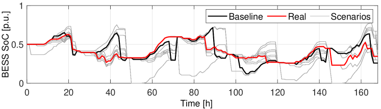
Figure 2: Results: BESS SoC profile.

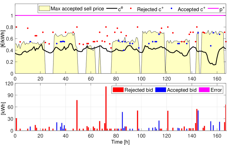
Figure 3: Results: REC sell bids: prices (top) and quantities (bottom).

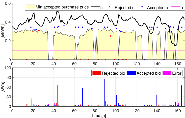
Figure 4: Results: REC purchase bids: prices (top) and quantities (bottom).

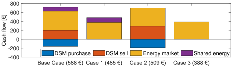
Figure 5: Results: REC cash flows. In brackets the total cash flow.

The one week simulation has been repeated in three different scenarios: Case 1, where the REC does not participate to the ACS; Case 2, where the incentive for shared energy $\gamma^{sh}$ is neglected; Case 3, where the incentive for shared energy $\gamma^{sh}$ is neglected and the REC does not participate in the ACS. The results are compared in terms of cash flows in Fig. 5. By this comparison it is possible to understand which is the actual advantage provided by the remuneration of shared energy and by the participation in ACS. Starting from Case 3: in Case 1 we obtain a cash flow increase of 25%, due to the sharing energy incentive; in Case 2 we get a cash flow increase of 31.2%, proving the profitability of the ACS participation. As expected the largest cash flow is realized in the base case, 21.2% more than Case 1, and 15.5% more than Case 3.

VI Conclusions

In this paper we have proposed a scenario-based day-ahead optimization algorithm for a REC participating in the Italian pay-as-bid ancillary service market. The algorithm is able to state the REC energy exchange baseline and decide the sell and purchase bids to be submitted to the service market with the objective of maximizing the REC cash flow. Simulation results prove the effectiveness of the approach and the advantages for the REC in participating in the service market.

References

- [1] European Union, “Directive (EU) 2018/2001 of the European Parliament and of the Council of 11 December 2018 on the promotion of the use of energy from renewable sources.” Official Journal of the European Union, vol. 61, 2018.
- [2] Italian Council of Ministers, “Decreto legislativo 8 novembre 2021, n. 199 attuazione della direttiva (UE) 2018/2001 del parlamento europeo e del consiglio, dell’11 dicembre 2018, sulla promozione dell’uso dell’energia da fonti rinnovabili,” 2021, [In Italian].
- [3] F. Conte, F. D’Antoni, G. Natrella, and M. Merone, “A new hybrid AI optimal management method for renewable energy communities,” Energy and AI, vol. 10, p. 100197, 2022.
- [4] F. R. Bianchi, B. Bosio, F. Conte, S. Massucco, G. Mosaico, G. Natrella, and M. Saviozzi, “Modelling and optimal management of renewable energy communities using reversible solid oxide cells,” Applied Energy, vol. 334, p. 120657, 2023.
- [5] G. Barone, G. Brusco, D. Menniti, A. Pinnarelli, G. Polizzi, N. Sorrentino, P. Vizza, and A. Burgio, “How smart metering and smart charging may help a local energy community in collective self-consumption in presence of electric vehicles,” Energies, vol. 13, no. 16, p. 4163, 2020.
- [6] D.-H. Park, J.-B. Park, K. Y. Lee, S.-Y. Son, and J. H. Roh, “A bidding-based peer-to-peer energy transaction model considering the green energy preference in virtual energy community,” IEEE Access, vol. 9, pp. 87 410–87 419, 2021.
- [7] F. Garcia-Munoz, F. Teng, A. Junyent-Ferre, F. Diaz-Gonzalez, and C. Corchero, “Stochastic energy community trading model for day-ahead and intraday coordination when offering DERs reactive power as ancillary services,” Sust. Energy, Grids and Networks, vol. 32, p. 100951, 2022.
- [8] Gestore dei Mercati Energetici, “Italian energy markets website.” [Online]. Available: https://www.mercatoelettrico.org/en/
- [9] N. Growe-Kuska, H. Heitsch, and W. Romisch, “Scenario reduction and scenario tree construction for power management problems,” in IEEE PowerTech, vol. 3, Bologna, Italy, 2003, pp. 1–7.
- [10] S. Massucco, G. Mosaico, M. Saviozzi, F. Silvestro, A. Fidigatti, and E. Ragaini, “An instantaneous growing stream clustering algorithm for probabilistic load modeling/profiling,” in 2020 Int. Conf. on Probabilistic Methods Applied to Power Systems (PMAPS), 2020, pp. 1–6.
- [11] P. Patrinos, S. Trimboli, and A. Bemporad, “Stochastic mpc for real-time market-based optimal power dispatch,” in 2011 IEEE CDC, 2011, pp. 7111–7116.
- [12] A. Bemporad, G. Ferrari-Trecate, and M. Morari, “Observability and controllability of piecewise affine and hybrid systems,” IEEE Transactions on Automatic Control, vol. 45, no. 10, pp. 1864–1876, 2000.
- [13] Gurobi Optimization, LLC, “Gurobi Optimizer Reference Manual,” 2023. [Online]. Available: https://www.gurobi.com
- [14] S. Ramos, J. Soares, Z. Foroozandeh, I. Tavares, and Z. Vale, “Energy consumption and PV generation data of 15 prosumers (15 minute resolution),” Zenodo, 2021. [Online]. Available: https://zenodo.org/records/5106455