Correlation Effects in a Trapped Bose-Fermi Mixture: Exact Results

Abstract

Many-body properties of a fermionic impurity embedded in a Bose-Einstein condensate are analyzed analytically using a solvable model, the harmonic-interaction model for Bose-Fermi mixtures. The one-particle and two-particle densities, reduced density matrices, and correlation functions of the fermions and bosons, both in position and momentum spaces, are prescribed in closed form. The various coherence lengths are analyzed. We show that the first-order coherence lengths in position and momentum spaces are equal whereas the second-order quantities can differ substantially. Illustrative examples where the sole interaction is between the impurity and the condensate are presented. Implications are briefly discussed.

1 Introduction

Ultracold atomic Bose-Fermi mixtures have generated a vast and extensive experimental and theoretical research for more than two decades, see, e.g., Refs. [1-32]. There are endless combinations, if one adds together intraspecies and interspecies interactions, numbers of particles of each species and their masses, and trapping potentials, to the inherent different nature of the Bose and Fermi statistics. On the theory side, this wealth offered by the ultracold realm makes solvable models rather scarce, especially in traps. The utility of exactly-solvable models of quantum many-particle systems is indispensable as tools to emulate such systems and to gain instincts on realistic scenarios. These are additional to the mere mathematical aesthetics which usually accompanies such models.

Harmonic-interaction models have amply been used to emulate many-particle systems for many years [33-52]. Another usage of harmonic-interaction models is to benchmark many-body theories and their numerical implementations [53-57]. The harmonic-interaction models have been mainly used for single-species bosons, single-species fermions, and Bose-Bose mixtures so far. In the present work we wish to add another brick to the building of harmonic-interaction models, and treat Bose-Fermi mixtures with it. Explicitly, we investigate analytically first-order and second-order correlations of a trapped fermionic impurity in a Bose-Einstein condensate both in position and momentum spaces. We build on derivations and results using the harmonic-interaction model for Bose-Fermi mixtures which will be reported in an extended format elsewhere [58].

2 Theory

The Bose-Fermi Hamiltonian within the harmonic-interaction model reads

$$\hat{H}(x_{1},\ldots,x_{N_{F}},y_{1},\ldots,y_{N_{B}})=$$

$$=\sum_{j=1}^{N_{F}}\left(-\frac{1}{2m_{F}}\frac{\partial^{2}}{\partial x_{j}^{2}}+\frac{1}{2}m_{F}\omega^{2}x_{j}^{2}\right)+\sum_{j=1}^{N_{B}}\left(-\frac{1}{2m_{B}}\frac{\partial^{2}}{\partial y_{j}^{2}}+\frac{1}{2}m_{B}\omega^{2}y_{j}^{2}\right)+$$

$$+\lambda_{F}\sum_{1\leq j<k}^{N_{F}}\left(x_{j}-x_{k}\right)^{2}+\lambda_{B}\sum_{1\leq j<k}^{N_{B}}\left(y_{j}-y_{k}\right)^{2}+\lambda_{BF}\sum_{j=1}^{N_{F}}\sum_{k=1}^{N_{B}}\left(x_{j}-y_{k}\right)^{2},\$$ (1)

where $N_{F},N_{B}$ are the numbers of fermions and bosons, $m_{F},m_{B}$ their masses, and $\lambda_{F},\lambda_{B}$ the intraspecies and $\lambda_{BF}$ the interspecies interactions strengths, respectively. Herein, the fermions are polarized.

Diagonalizing (2) leads to four distinct eigenfrequencies, also see the Bose-Bose mixture [45, 50]

$$\Omega_{F}=\sqrt{\omega^{2}+\frac{2}{m_{F}}\left(N_{F}\lambda_{F}+N_{B}\lambda_{BF}\right)},\qquad\Omega_{B}=\sqrt{\omega^{2}+\frac{2}{m_{B}}\left(N_{B}\lambda_{B}+N_{F}\lambda_{BF}\right)},$$

$$\Omega_{BF}=\sqrt{\omega^{2}+2\left(\frac{N_{B}}{m_{F}}+\frac{N_{F}}{m_{B}}\right)\lambda_{BF}},\qquad\omega.\$$ (2)

The ground-state energy of $N_{F}$ fermions and $N_{B}$ bosons is [58]

$$E=\frac{1}{2}\Bigg{[}\left(N_{F}^{2}-1\right)\sqrt{\omega^{2}+\frac{2}{m_{F}}(N_{F}\lambda_{F}+N_{B}\lambda_{BF})}+$$

$$+\left(N_{B}-1\right)\sqrt{\omega^{2}+\frac{2}{m_{B}}(N_{B}\lambda_{B}+N_{F}\lambda_{BF})}+\sqrt{\omega^{2}+2\left(\frac{N_{B}}{m_{F}}+\frac{N_{F}}{m_{B}}\right)\lambda_{BF}}+\omega\Bigg{]},$$ (3)

and the wavefunction in Cartesian coordinates reads

$$\Psi(x_{1},\ldots,x_{N_{F}},y_{1},\ldots,y_{N_{B}})=$$

$$={\mathcal{N}}\left(\frac{m_{F}\Omega_{F}}{\pi}\right)^{\frac{N_{F}^{2}-1}{4}}\left(\frac{m_{B}\Omega_{B}}{\pi}\right)^{\frac{N_{B}-1}{4}}\left(\frac{M_{BF}\Omega_{BF}}{\pi}\right)^{\frac{1}{4}}\left(\frac{M\omega}{\pi}\right)^{\frac{1}{4}}\times$$

$$\times\left[\prod_{1\leq j<k\leq N_{F}}\left(x_{j}-x_{k}\right)\right]e^{-\frac{\alpha_{F}}{2}\sum_{j=1}^{N_{F}}x_{j}^{2}-\beta_{F}\sum_{1\leq j<k}^{N_{F}}x_{j}x_{k}}e^{-\frac{\alpha_{B}}{2}\sum_{j=1}^{N_{B}}y_{j}^{2}-\beta_{B}\sum_{1\leq j<k}^{N_{B}}y_{j}y_{k}}\times$$

$$\times e^{+\gamma\sum_{j=1}^{N_{F}}\sum_{k=1}^{N_{B}}x_{j}y_{k}},\$$ (4)

where $\prod_{1\leq j<k\leq N_{F}}\left(x_{j}-x_{k}\right)=V(x_{1},\ldots,x_{N_{F}})$ is the Vandermonde determinant and ${\mathcal{N}}$ is a dimensionless normalization constant that appears in the derivation due to the relative Jacoby coordinates of the fermions [58]. The center-of-mass and relative center-of-mass degrees-of-freedom have the masses $M=m_{F}N_{F}+m_{B}N_{B}$ and $M_{BF}=\frac{m_{F}n_{B}}{M}$, respectively.

There are five coefficients in the wavefunction, also see [50],

$$\alpha_{F}=m_{F}\Omega_{F}\left[1+\frac{1}{N_{F}}\left(\frac{m_{F}N_{F}}{M}\frac{\omega}{\Omega_{F}}+\frac{m_{B}N_{B}}{M}\frac{\Omega_{BF}}{\Omega_{F}}-1\right)\right],\qquad\beta_{F}=\alpha_{F}-m_{F}\Omega_{F},$$

$$\alpha_{B}=m_{B}\Omega_{B}\left[1+\frac{1}{N_{B}}\left(\frac{m_{B}N_{B}}{M}\frac{\omega}{\Omega_{B}}+\frac{m_{F}N_{F}}{M}\frac{\Omega_{BF}}{\Omega_{B}}-1\right)\right],\qquad\beta_{B}=\alpha_{B}-m_{B}\Omega_{B},$$

$$\gamma=\frac{m_{F}m_{B}}{M}(\Omega_{BF}-\omega),\$$ (5)

which are used to express and evaluate all the correlation properties in the Bose-Fermi mixture. Explicitly, the reduced one-particle and two-particle density matrices [59, 60] and Glauber’s normalized first-order and second-order correlation functions [61-63] of the fermions and bosons, both in position and momentum spaces, are put forward in closed form and investigated.

2.1 Position and momentum correlation functions of the bosons

Consider an impurity consisting of $N_{F}=2$ fermions embedded in a Bose-Einstein condensate made of $N_{B}$ bosons. Two fermions in the impurity already lead to rich results. Of course, this is the minimal number of indistinguishable particles to exhibit the antisymmetry of the wavefunction (2) under their exchange. The results for fermions obtained below are hence explicit to two fermions, although some of them hold for a general number $N_{F}$ of fermions. It is instructive to analyze the condensate first and than the impurity, since the bosons’ correlation functions are relatively simpler than the fermions’ ones.

The reduced one-particle density matrix and the density of the bosons in position space are integrated from the all-particle density matrix and read [50, 58]

$$\rho^{(1)}_{B}(y,y^{\prime})=N_{B}\left(\frac{\alpha_{B}+C^{\prime}_{0,1}}{\pi}\right)^{\frac{1}{2}}e^{-\frac{\alpha_{B}+C^{\prime}_{0,1}}{4}\left(y+y^{\prime}\right)^{2}}e^{-\frac{\alpha_{B}}{4}\left(y-y^{\prime}\right)^{2}},$$

$$\rho^{(1)}_{B}(y)=N_{B}\left(\frac{\alpha_{B}+C^{\prime}_{0,1}}{\pi}\right)^{\frac{1}{2}}e^{-\left(\alpha_{B}+C^{\prime}_{0,1}\right)y^{2}}.\$$ (6)

We can now compute explicitly from (2.1) the first-order correlation function in position space,

$$g_{B}^{(1)}(y,y^{\prime})=\frac{\rho^{(1)}_{B}(y,y^{\prime})}{\sqrt{\rho^{(1)}_{B}(y)\rho^{(1)}_{B}(y^{\prime})}}=e^{-\frac{-C^{\prime}_{0,1}}{4}\left(y-y^{\prime}\right)^{2}},\$$ (7)

where $C^{\prime}_{0,1}$ is negative and given in closed form as a function of the coefficients (2) [50, 58], see below.

It is useful to define a dimensionless measure, the first-order coherence length in position space, as the ratio of the off-diagonal decay length of the first-order correlation function (7) and the diagonal decay length of the reduced one-particle density matrix (2.1), see [58],

$$l_{B}^{(1)}=\sqrt{\frac{\alpha_{B}+C^{\prime}_{0,1}}{-C^{\prime}_{0,1}}}=\frac{1}{\sqrt{\left(\frac{1+\rho_{B}^{(1)}}{1-\rho_{B}^{(1)}}\right)^{2}-1}}=$$ (8)

$$=\frac{1}{\sqrt{\left[1+\frac{1}{N_{B}}\left(\frac{m_{B}N_{B}}{M}\frac{\omega}{\Omega_{B}}+\frac{m_{F}N_{F}}{M}\frac{\Omega_{BF}}{\Omega_{B}}-1\right)\right]\left[1+\frac{1}{N_{B}}\left(\frac{m_{B}N_{B}}{M}\frac{\Omega_{B}}{\omega}+\frac{m_{F}N_{F}}{M}\frac{\Omega_{B}}{\Omega_{BF}}-1\right)\right]-1}}.\$$

The second expression of $l_{B}^{(1)}$ in (8) is because it is possible to express the first-order coherence length using the depleted fraction $0\leq\rho_{B}^{(1)}<1$. The depleted fraction is given in closed-form using the above coefficients, $\rho_{B}^{(1)}=\frac{\sqrt{\alpha_{B}}-\sqrt{\alpha_{B}+C^{\prime}_{0,1}}}{\sqrt{\alpha_{B}}+\sqrt{\alpha_{B}+C^{\prime}_{0,1}}}$, see [51]. Clearly the coherence length $l_{B}^{(1)}$ diverges for non-interacting bosons when there is no depletion [$\rho_{B}^{(1)}=0$]. Illustrative examples and further discussion are given in Sec. 3.

Let us proceed and compute the reduced one-particle density matrix and the density of the bosons in momentum space,

$$\tilde{\rho}^{(1)}_{B}(q,q^{\prime})=\frac{1}{2\pi}\int dydy^{\prime}e^{-i\left(qy-q^{\prime}y^{\prime}\right)}\rho^{(1)}_{B}(y,y^{\prime})=$$

$$=N_{B}\left(\frac{1}{\pi\alpha_{B}}\right)^{\frac{1}{2}}e^{-\frac{1}{4\alpha_{B}}\left(q+q^{\prime}\right)^{2}}e^{-\frac{1}{4\left(\alpha_{B}+C^{\prime}_{0,1}\right)}\left(q-q^{\prime}\right)^{2}},$$

$$\tilde{\rho}^{(1)}_{B}(q)=N_{B}\left(\frac{1}{\pi\alpha_{B}}\right)^{\frac{1}{2}}e^{-\frac{1}{\alpha_{B}}q^{2}}.\$$ (9)

Consequently, just like (7), the first-order correlation function in momentum space is readily obtained

$$\tilde{g}_{B}^{(1)}(q,q^{\prime})=\frac{\tilde{\rho}^{(1)}_{B}(q,q^{\prime})}{\sqrt{\tilde{\rho}^{(1)}_{B}(q)\tilde{\rho}^{(1)}_{B}(q^{\prime})}}=e^{-\frac{-C^{\prime}_{0,1}}{4\alpha_{B}\left(\alpha_{B}+C^{\prime}_{0,1}\right)}\left(q-q^{\prime}\right)^{2}}.\$$ (10)

Analogously to (8), we define a dimensionless measure, the first-order coherence length in momentum space, as the ratio of the off-diagonal decay length of the first-order correlation function (10) and the diagonal decay length of the reduced one-particle density matrix (2.1), both in momentum space,

$$\tilde{l}_{B}^{(1)}=\sqrt{\frac{\alpha_{B}+C^{\prime}_{0,1}}{-C^{\prime}_{0,1}}}=l_{B}^{(1)}.$$ (11)

We find that the first-order coherence lengths in position (8) and momentum (11) spaces are equal.

To facilitate the Fourier transform of second-order quantities to momentum space later on, the reduced two-particle density matrix in position space is written in a quadratic form using normal coordinates as follows

$$\rho_{B}^{(2)}(y_{1},y^{\prime}_{1},y_{2},y^{\prime}_{2})=N_{B}(N_{B}-1)\left[\frac{\left(\alpha_{B}-\beta_{B}\right)\left(\alpha_{B}+\beta_{B}+2C^{\prime}_{0,2}\right)}{\pi^{2}}\right]^{\frac{1}{2}}\times$$

$$\times e^{-\frac{\alpha_{B}+\beta_{B}+2C^{\prime}_{0,2}}{8}\left(y_{1}+y_{2}+y^{\prime}_{1}+y^{\prime}_{2}\right)^{2}}e^{-\frac{\alpha_{B}-\beta_{B}}{8}\left(y_{1}-y_{2}+y^{\prime}_{1}-y^{\prime}_{2}\right)^{2}}\times$$

$$\times e^{-\frac{\alpha_{B}+\beta_{B}}{8}\left(y_{1}+y_{2}-y^{\prime}_{1}-y^{\prime}_{2}\right)^{2}}e^{-\frac{\alpha_{B}-\beta_{B}}{8}\left(y_{1}-y_{2}-y^{\prime}_{1}+y^{\prime}_{2}\right)^{2}},$$

$$\rho_{B}^{(2)}(y_{1},y_{2})=N_{B}(N_{B}-1)\left[\frac{\left(\alpha_{B}-\beta_{B}\right)\left(\alpha_{B}+\beta_{B}+2C^{\prime}_{0,2}\right)}{\pi^{2}}\right]^{\frac{1}{2}}\times$$

$$\times e^{-\frac{1}{2}\left(\alpha_{B}+\beta_{B}+2C^{\prime}_{0,2}\right)\left(y_{1}+y_{2}\right)^{2}}e^{-\frac{1}{2}\left(\alpha_{B}-\beta_{B}\right)\left(y_{1}-y_{2}\right)^{2}},\$$ (12)

from which its diagonal, the two-body density in position space, is given [51, 58].

Next, the second-order correlation function in position space reads

$$g_{B}^{(2)}(y_{1},y_{2})=\frac{\rho^{(2)}_{B}(y_{1},y_{2})}{\rho^{(1)}_{B}(y_{1})\rho^{(1)}_{B}(y_{2})}=\frac{N_{B}-1}{N_{B}}\left[\frac{\left(\alpha_{B}+C^{\prime}_{0,2}\right)^{2}}{\left(\alpha_{B}-\beta_{B}\right)\left(\alpha_{B}+\beta_{B}+2C^{\prime}_{0,2}\right)}\right]^{\frac{1}{2}}\times$$

$$\times e^{-\frac{1}{2}\frac{-\left(\alpha_{B}-\beta_{B}\right)\left(\beta_{B}+C^{\prime}_{0,2}\right)}{\alpha_{B}+C^{\prime}_{0,2}}\left(y_{1}-y_{2}\right)^{2}}e^{+\frac{1}{2}\frac{-\left(\alpha_{B}+\beta_{B}+2C^{\prime}_{0,2}\right)\left(\beta_{B}+C^{\prime}_{0,2}\right)}{\alpha_{B}+C^{\prime}_{0,2}}\left(y_{1}+y_{2}\right)^{2}}.\$$ (13)

For $\beta_{B}+C^{\prime}_{0,2}<0$ the off diagonal decays and the diagonal grows, and for $\beta_{B}+C^{\prime}_{0,2}>0$ vice versa, also see the applications in Sec. 3 and A.

We can now proceed and define a dimensionless measure, the second-order coherence length in position space, as the ratio of the off-diagonal decay or growth length of the second-order correlation function (2.1) and the diagonal decay length of the two-particle density (2.1),

$$l_{B}^{(2)}=\sqrt{\frac{\left(\alpha_{B}+\beta_{B}+2C^{\prime}_{0,2}\right)\left(\alpha_{B}+C^{\prime}_{0,2}\right)}{\left(\alpha_{B}-\beta_{B}\right)|\beta_{B}+C^{\prime}_{0,2}|}}=$$ (14)

$$=\sqrt{\frac{1+\frac{1}{N_{B}}\left(\frac{m_{B}N_{B}}{M}\frac{\Omega_{B}}{\omega}+\frac{m_{F}N_{F}}{M}\frac{\Omega_{B}}{\Omega_{BF}}-1\right)}{\left[1+\frac{2}{N_{B}}\left(\frac{m_{B}N_{B}}{M}\frac{\Omega_{B}}{\omega}+\frac{m_{F}N_{F}}{M}\frac{\Omega_{B}}{\Omega_{BF}}-1\right)\right]\left|\frac{1}{N_{B}}\left(\frac{m_{B}N_{B}}{M}\frac{\Omega_{B}}{\omega}+\frac{m_{F}N_{F}}{M}\frac{\Omega_{B}}{\Omega_{BF}}-1\right)\right|}}.\$$

It is instrumental to compare the first-order $l_{B}^{(1)}$ and second-order $l_{B}^{(2)}$ coherence lengths, also see the illustrative examples in Sec. 3.

We now proceed to compute the the reduced two-particle density matrix and its diagonal, the two-body density of the bosons, in momentum space which take on the form

$$\tilde{\rho}_{B}^{(2)}(q_{1},q^{\prime}_{1},q_{2},q^{\prime}_{2})=\frac{1}{\left(2\pi\right)^{2}}\int dy_{1}dy_{2}dy^{\prime}_{1}dy^{\prime}_{2}e^{-i\left(q_{1}y_{1}+q_{2}y_{2}-q^{\prime}_{1}y^{\prime}_{1}-q^{\prime}_{2}y^{\prime}_{2}\right)}\rho_{B}^{(2)}(y_{1},y^{\prime}_{1},y_{2},y^{\prime}_{2})=$$ (15)

$$=N_{B}(N_{B}-1)\frac{1}{\pi\sqrt{\alpha_{B}^{2}-\beta^{2}_{B}}}e^{-\frac{1}{8\left(\alpha_{B}+\beta_{B}\right)}\left(q_{1}+q_{2}+q^{\prime}_{1}+q^{\prime}_{2}\right)^{2}}e^{-\frac{1}{8\left(\alpha_{B}-\beta_{B}\right)}\left(q_{1}-q_{2}+q^{\prime}_{1}-q^{\prime}_{2}\right)^{2}}\times$$

$$\times e^{-\frac{1}{8\left(\alpha_{B}+\beta_{B}+2C^{\prime}_{0,2}\right)}\left(q_{1}+q_{2}-q^{\prime}_{1}-q^{\prime}_{2}\right)^{2}}e^{-\frac{1}{8\left(\alpha_{B}-\beta_{B}\right)}\left(q_{1}-q_{2}-q^{\prime}_{1}+q^{\prime}_{2}\right)^{2}},$$

$$\tilde{\rho}_{B}^{(2)}(q_{1},q_{2})=N_{B}(N_{B}-1)\frac{1}{\pi\sqrt{\alpha_{B}^{2}-\beta^{2}_{B}}}e^{-\frac{1}{2\left(\alpha_{B}+\beta_{B}\right)}\left(q_{1}+q_{2}\right)^{2}}e^{-\frac{1}{2\left(\alpha_{B}-\beta_{B}\right)}\left(q_{1}-q_{2}\right)^{2}}.\$$

Then, the second-order correlation function of the bosons in momentum space can readily be evaluated as

$$\tilde{g}_{B}^{(2)}(q_{1},q_{2})=\frac{\tilde{\rho}^{(2)}_{B}(q_{1},q_{2})}{\tilde{\rho}^{(1)}_{B}(q_{1})\tilde{\rho}^{(1)}_{B}(q_{2})}=$$

$$=\frac{N_{B}-1}{N_{B}}\sqrt{\frac{\alpha_{B}^{2}}{\alpha_{B}^{2}-\beta_{B}^{2}}}e^{-\frac{1}{2}\frac{\beta_{B}}{\alpha_{B}\left(\alpha_{B}-\beta_{B}\right)}\left(q_{1}-q_{2}\right)^{2}}e^{+\frac{1}{2}\frac{\beta_{B}}{\alpha_{B}\left(\alpha_{B}+\beta_{B}\right)}\left(q_{1}+q_{2}\right)^{2}}.\$$ (16)

For $\beta_{B}>0$ the off diagonal decays and the diagonal grows, and for $\beta_{B}<0$ vice versa, also see the illustrative examples and A below.

Analogously to (14), we define a dimensionless measure, the second-order coherence length in momentum space, as the ratio of the off-diagonal decay or growth length of the second-order correlation function (2.1) and the diagonal decay length of the two-particle density (15), both in momentum space,

$$\!\!\!\!\!\!\!\!\tilde{l}_{B}^{(2)}=\sqrt{\frac{\alpha_{B}\left(\alpha_{B}-\beta_{B}\right)}{|\beta_{B}|\left(\alpha_{B}+\beta_{B}\right)}}=$$ (17)

$$\!\!\!\!\!\!\!\!=\sqrt{\frac{1+\frac{1}{N_{B}}\left(\frac{m_{B}N_{B}}{M}\frac{\omega}{\Omega_{B}}+\frac{m_{F}N_{F}}{M}\frac{\Omega_{BF}}{\Omega_{B}}-1\right)}{\left[1+\frac{2}{N_{B}}\left(\frac{m_{B}N_{B}}{M}\frac{\omega}{\Omega_{B}}+\frac{m_{F}N_{F}}{M}\frac{\Omega_{BF}}{\Omega_{B}}-1\right)\right]\left|\frac{1}{N_{B}}\left(\frac{m_{B}N_{B}}{M}\frac{\omega}{\Omega_{B}}+\frac{m_{F}N_{F}}{M}\frac{\Omega_{BF}}{\Omega_{B}}-1\right)\right|}}\neq l_{B}^{(2)}.\$$

It is found that the second-order coherence lengths in position (14) and momentum (17) spaces are different, unlike the respective first-order coherence lengths. The reason is that different parts of the many-particle wavefunction contribute to the second-order quantities in position and momentum spaces. Although $l_{B}^{(1)}\neq\tilde{l}_{B}^{(1)}$, their respective expressions are ‘reciprocal’ to each other in the sense $\frac{\Omega_{B}}{\omega},\frac{\Omega_{B}}{\Omega_{BF}}\Leftrightarrow\frac{\omega}{\Omega_{B}},\frac{\Omega_{BF}}{\Omega_{B}}$, see above and compare (14) and (17). Additionally and on the other hand, there seems to be no simple relation between the second-order coherence lengths and the pair depleted fraction $0\leq\rho_{B}^{(2)}<1$. For reference, the pair depleted fraction is given in closed-form using the above coefficients and reads $\rho_{B}^{(2)}=\frac{\sqrt{\alpha_{B}+\beta_{B}}-\sqrt{\alpha_{B}+\beta_{B}+2C^{\prime}_{0,2}}}{\sqrt{\alpha_{B}+\beta_{B}}+\sqrt{\alpha_{B}+\beta_{B}+2C^{\prime}_{0,2}}}$, see [51]. Last but not least, it is deductive to compare the first-order $\tilde{l}_{B}^{(1)}$ and second-order $\tilde{l}_{B}^{(2)}$ coherence lengths in momentum space as well, also see the illustrative examples in Sec. 3.

2.2 Position and momentum correlation functions of the fermions

The reduced one-particle density matrix and the density of the $N_{F}=2$ fermions in position space read [58]

$$\!\!\!\!\!\!\!\!\rho_{F}^{(1)}(x,x^{\prime})=2\left(\frac{\alpha_{F}+C_{1,0}}{\pi}\right)^{\frac{1}{2}}\times$$ (18)

$$\!\!\!\!\!\!\!\!\times\left\{1-\frac{1}{2}\frac{\alpha_{F}+C_{1,0}}{\alpha_{F}-\beta_{F}}+\frac{1}{4}\left[\frac{\left(\alpha_{F}+C_{1,0}\right)^{2}}{\alpha_{F}-\beta_{F}}\left(x+x^{\prime}\right)^{2}-\left(\alpha_{F}-\beta_{F}\right)\left(x-x^{\prime}\right)^{2}\right]\right\}\times$$

$$\!\!\!\!\!\!\!\!\times e^{-\frac{\alpha_{F}+C_{1,0}}{4}\left(x+x^{\prime}\right)^{2}}e^{-\frac{\alpha_{F}}{4}\left(x-x^{\prime}\right)^{2}},$$

$$\!\!\!\!\!\!\!\!\rho_{F}^{(1)}(x)=2\left(\frac{\alpha_{F}+C_{1,0}}{\pi}\right)^{\frac{1}{2}}\left[1-\frac{1}{2}\frac{\alpha_{F}+C_{1,0}}{\alpha_{F}-\beta_{F}}+\frac{\left(\alpha_{F}+C_{1,0}\right)^{2}}{\alpha_{F}-\beta_{F}}x^{2}\right]e^{-\left(\alpha_{F}+C_{1,0}\right)x^{2}}.\$$

Using (18), the first-order correlation function of the fermions in position space is computed as

$$\!\!\!\!\!\!\!\!g_{F}^{(1)}(x,x^{\prime})=\frac{\rho^{(1)}_{F}(x,x^{\prime})}{\sqrt{\rho^{(1)}_{F}(x)\rho^{(1)}_{F}(x^{\prime})}}=$$

$$\!\!\!\!\!\!\!\!=\frac{1-\frac{1}{2}\frac{\alpha_{F}+C_{1,0}}{\alpha_{F}-\beta_{F}}+\frac{1}{4}\left[\frac{\left(\alpha_{F}+C_{1,0}\right)^{2}}{\alpha_{F}-\beta_{F}}\left(x+x^{\prime}\right)^{2}-\left(\alpha_{F}-\beta_{F}\right)\left(x-x^{\prime}\right)^{2}\right]}{\sqrt{\left[1-\frac{1}{2}\frac{\alpha_{F}+C_{1,0}}{\alpha_{F}-\beta_{F}}+\frac{\left(\alpha_{F}+C_{1,0}\right)^{2}}{\alpha_{F}-\beta_{F}}x^{2}\right]\left[1-\frac{1}{2}\frac{\alpha_{F}+C_{1,0}}{\alpha_{F}-\beta_{F}}+\frac{\left(\alpha_{F}+C_{1,0}\right)^{2}}{\alpha_{F}-\beta_{F}}{x^{\prime}}^{2}\right]}}e^{-\frac{-C_{1,0}}{4}\left(x-x^{\prime}\right)^{2}},\$$ (19)

where $C_{1,0}$ is negative and given in closed form as a function of the coefficients (2) [50, 58], see for further discussion below.

Similarly to the bosons, it is instructive to define a dimensionless measure, the first-order coherence length of the fermions in position space, as the ratio of the off-diagonal decay length of the first-order correlation function (2.2) and the diagonal decay length of the reduced one-particle density matrix (18), giving

$$l_{F}^{(1)}=\sqrt{\frac{\alpha_{F}+C_{1,0}}{-C_{1,0}}}=$$ (20)

$$=\frac{1}{\sqrt{\left[1+\frac{1}{N_{F}}\left(\frac{m_{F}N_{F}}{M}\frac{\omega}{\Omega_{F}}+\frac{m_{B}N_{B}}{M}\frac{\Omega_{BF}}{\Omega_{F}}-1\right)\right]\left[1+\frac{1}{N_{F}}\left(\frac{m_{F}N_{F}}{M}\frac{\Omega_{F}}{\omega}+\frac{m_{B}N_{B}}{M}\frac{\Omega_{F}}{\Omega_{BF}}-1\right)\right]-1}}.\$$

Formally, it is possible to re-express the first-order coherence length (20) using the quantity $\bar{\rho}_{F}^{(1)}=\frac{\sqrt{\alpha_{F}}-\sqrt{\alpha_{F}+C_{1,0}}}{\sqrt{\alpha_{F}}+\sqrt{\alpha_{F}+C_{1,0}}}$, which satisfies $0\leq\bar{\rho}_{F}^{(1)}<1$ and which would have been the depleted fraction if the impurity were bosonic, see [51]. The final result is $l_{F}^{(1)}=\left[\left(\frac{1+\bar{\rho}_{F}^{(1)}}{1-\bar{\rho}_{F}^{(1)}}\right)^{2}-1\right]^{-\frac{1}{2}}$, compare to (8). Obviously, the first-order coherence length $l_{F}^{(1)}$ diverges for non-interacting fermions.

The reduced one-particle density matrix and the density of the fermions in momentum space are readily evaluated from the reduced one-particle density matrix in position space,

$$\!\!\!\!\!\!\!\!\tilde{\rho}_{F}^{(1)}(k,k^{\prime})=\frac{1}{2\pi}\int dxdx^{\prime}e^{-i\left(kx-k^{\prime}x^{\prime}\right)}\rho^{(1)}_{F}(x,x^{\prime})=$$

$$\!\!\!\!\!\!\!\!=2\left(\frac{1}{\pi\alpha_{F}}\right)^{\frac{1}{2}}\left\{1-\frac{1}{2}\frac{\alpha_{F}-\beta_{F}}{\alpha_{F}}+\frac{1}{4}\left[\frac{\alpha_{F}-\beta_{F}}{\alpha_{F}^{2}}\left(k+k^{\prime}\right)^{2}-\frac{1}{\alpha_{F}-\beta_{F}}\left(k-k^{\prime}\right)^{2}\right]\right\}\times$$

$$\!\!\!\!\!\!\!\!\times e^{-\frac{1}{4\alpha_{F}}\left(k+k^{\prime}\right)^{2}}e^{-\frac{1}{4\left(\alpha_{F}+C_{1,0}\right)}\left(k-k^{\prime}\right)^{2}},$$

$$\!\!\!\!\!\!\!\!\tilde{\rho}_{F}^{(1)}(k)=2\left(\frac{1}{\pi\alpha_{F}}\right)^{\frac{1}{2}}\left[1-\frac{1}{2}\frac{\alpha_{F}-\beta_{F}}{\alpha_{F}}+\frac{\alpha_{F}-\beta_{F}}{\alpha_{F}^{2}}k^{2}\right]e^{-\frac{1}{\alpha_{F}}k^{2}}.\$$ (21)

Afterwards, the first-order correlation function in momentum space is given by

$$\!\!\!\!\!\!\!\!\tilde{g}_{F}^{(1)}(k,k^{\prime})=\frac{\tilde{\rho}^{(1)}_{F}(k,k^{\prime})}{\sqrt{\tilde{\rho}^{(1)}_{F}(k)\tilde{\rho}^{(1)}_{F}(k^{\prime})}}=$$

$$\!\!\!\!\!\!\!\!=\frac{1-\frac{1}{2}\frac{\alpha_{F}-\beta_{F}}{\alpha_{F}}+\frac{1}{4}\left[\frac{\alpha_{F}-\beta_{F}}{\alpha_{F}^{2}}\left(k+k^{\prime}\right)^{2}-\frac{1}{\alpha_{F}-\beta_{F}}\left(k-k^{\prime}\right)^{2}\right]}{\sqrt{\left[1-\frac{1}{2}\frac{\alpha_{F}-\beta_{F}}{\alpha_{F}}+\frac{\alpha_{F}-\beta_{F}}{\alpha_{F}^{2}}k^{2}\right]\left[1-\frac{1}{2}\frac{\alpha_{F}-\beta_{F}}{\alpha_{F}}+\frac{\alpha_{F}-\beta_{F}}{\alpha_{F}^{2}}{k^{\prime}}^{2}\right]}}e^{-\frac{-C_{1,0}}{4\alpha_{F}\left(\alpha_{F}+C_{1,0}\right)}\left(k-k^{\prime}\right)^{2}}.\$$ (22)

Just like (11), we define a dimensionless measure, the first-order coherence length of the fermions in momentum space, as the ratio of the off-diagonal decay length of the first-order correlation function (2.2) and the diagonal decay length of the reduced one-particle density matrix (2.2), both in momentum space,

$$\tilde{l}_{F}^{(1)}=\sqrt{\frac{\alpha_{F}+C_{1,0}}{-C_{1,0}}}=l_{F}^{(1)}.$$ (23)

It is found that the first-order coherence lengths in position (20) and momentum (23) spaces are equal.

To ease the Fourier transform of second-order quantities to momentum space below, the reduced two-particle density matrix in position space, including the term $\left(x_{1}-x_{2}\right)\left(x^{\prime}_{1}-x^{\prime}_{2}\right)$, is expressed in a quadratic form using normal coordinates. The final result is given by

$$\rho_{F}^{(2)}(x_{1},x^{\prime}_{1},x_{2},x^{\prime}_{2})=2\left[\frac{\left(\alpha_{F}-\beta_{F}\right)^{3}\left(\alpha_{F}+\beta_{F}+2C_{2,0}\right)}{\pi^{2}}\right]^{\frac{1}{2}}\times$$

$$\times\left(x_{1}-x_{2}\right)\left(x^{\prime}_{1}-x^{\prime}_{2}\right)e^{-\frac{\alpha_{F}+\beta_{F}+2C_{2,0}}{8}\left(x_{1}+x_{2}+x^{\prime}_{1}+x^{\prime}_{2}\right)^{2}}e^{-\frac{\alpha_{F}-\beta_{F}}{8}\left(x_{1}-x_{2}+x^{\prime}_{1}-x^{\prime}_{2}\right)^{2}}\times$$

$$\times e^{-\frac{\alpha_{F}+\beta_{F}}{8}\left(x_{1}+x_{2}-x^{\prime}_{1}-x^{\prime}_{2}\right)^{2}}e^{-\frac{\alpha_{F}-\beta_{F}}{8}\left(x_{1}-x_{2}-x^{\prime}_{1}+x^{\prime}_{2}\right)^{2}},$$

$$\rho_{F}^{(2)}(x_{1},x_{2})=2\left[\frac{\left(\alpha_{F}-\beta_{F}\right)^{3}\left(\alpha_{F}+\beta_{F}+2C_{2,0}\right)}{\pi^{2}}\right]^{\frac{1}{2}}\times$$

$$\times\left(x_{1}-x_{2}\right)^{2}e^{-\frac{1}{2}\left(\alpha_{F}+\beta_{F}+2C_{2,0}\right)\left(x_{1}+x_{2}\right)^{2}}e^{-\frac{1}{2}\left(\alpha_{F}-\beta_{F}\right)\left(x_{1}-x_{2}\right)^{2}},\$$ (24)

from which the two-body density in position space is prescribed.

The second-order correlation function in position space is now evaluated as

$$g_{F}^{(2)}(x_{1},x_{2})=\frac{\rho^{(2)}_{F}(x_{1},x_{2})}{\rho^{(1)}_{F}(x_{1})\rho^{(1)}_{F}(x_{2})}=\frac{1}{2}\left[\frac{\left(\alpha_{F}+C_{2,0}\right)^{2}}{\left(\alpha_{F}-\beta_{F}\right)^{3}\left(\alpha_{F}+\beta_{F}+2C_{2,0}\right)}\right]^{\frac{1}{2}}\times$$

$$\times\frac{\left(x_{1}-x_{2}\right)^{2}}{\left[\frac{1}{2\left(\alpha_{F}+C_{2,0}\right)}+\left(1+\frac{\beta_{F}+C_{2,0}}{\alpha_{F}+C_{2,0}}\right)^{2}x_{1}^{2}\right]\left[\frac{1}{2\left(\alpha_{F}+C_{2,0}\right)}+\left(1+\frac{\beta_{F}+C_{2,0}}{\alpha_{F}+C_{2,0}}\right)^{2}x_{2}^{2}\right]}\times$$

$$\times e^{-\frac{1}{2}\frac{-\left(\alpha_{F}-\beta_{F}\right)\left(\beta_{F}+C_{2,0}\right)}{\alpha_{F}+C_{2,0}}\left(x_{1}-x_{2}\right)^{2}}e^{+\frac{1}{2}\frac{-\left(\alpha_{F}+\beta_{F}+2C_{2,0}\right)\left(\beta_{F}+C_{2,0}\right)}{\alpha_{F}+C_{2,0}}\left(x_{1}+x_{2}\right)^{2}}.\$$ (25)

For $\beta_{F}+C_{2,0}<0$ the off diagonal decays and the diagonal grows whereas the opposite occurs for $\beta_{F}+C_{2,0}>0$, also see Sec. 3 and A below.

We define and compute a dimensionless measure, the second-order coherence length of the fermions in position space, as the ratio of the off-diagonal decay or growth length of the second-order correlation function (2.2) and the diagonal decay length of the two-particle density (2.2),

$$l_{F}^{(2)}=\sqrt{\frac{\left(\alpha_{F}+\beta_{F}+2C_{2,0}\right)\left(\alpha_{F}+C_{2,0}\right)}{\left(\alpha_{F}-\beta_{F}\right)|\beta_{F}+C_{2,0}|}}=$$ (26)

$$=\sqrt{\frac{1+\frac{1}{N_{F}}\left(\frac{m_{F}N_{F}}{M}\frac{\Omega_{F}}{\omega}+\frac{m_{B}N_{B}}{M}\frac{\Omega_{F}}{\Omega_{BF}}-1\right)}{\left[1+\frac{2}{N_{F}}\left(\frac{m_{F}N_{F}}{M}\frac{\Omega_{F}}{\omega}+\frac{m_{B}N_{B}}{M}\frac{\Omega_{F}}{\Omega_{BF}}-1\right)\right]\left|\frac{1}{N_{F}}\left(\frac{m_{F}N_{F}}{M}\frac{\Omega_{F}}{\omega}+\frac{m_{B}N_{B}}{M}\frac{\Omega_{F}}{\Omega_{BF}}-1\right)\right|}}.\$$

It would be instructive to contrast the first-order $l_{F}^{(1)}$ and second-order $l_{F}^{(2)}$ coherence lengths, which is done in the illustrative examples of Sec. 3.

To continue, the reduced two-particle density matrix and two-body density of the fermions in momentum space are calculated,

$$\!\!\!\!\!\!\!\!\!\!\!\!\!\!\!\!\tilde{\rho}_{F}^{(2)}(k_{1},k^{\prime}_{1},k_{2},k^{\prime}_{2})=\frac{1}{\left(2\pi\right)^{2}}\int dx_{1}dx_{2}dx^{\prime}_{1}dx^{\prime}_{2}e^{-i\left(k_{1}x_{1}+k_{2}x_{2}-k^{\prime}_{1}x^{\prime}_{1}-k^{\prime}_{2}x^{\prime}_{2}\right)}\rho_{F}^{(2)}(x_{1},x^{\prime}_{1},x_{2},x^{\prime}_{2})=$$

$$\!\!\!\!\!\!\!\!\!\!\!\!\!\!\!\!=2\frac{1}{\pi\sqrt{\left(\alpha_{F}^{2}-\beta^{2}_{F}\right)\left(\alpha_{F}-\beta_{F}\right)^{2}}}\left(k_{1}-k_{2}\right)\left(k^{\prime}_{1}-k^{\prime}_{2}\right)e^{-\frac{1}{8\left(\alpha_{F}+\beta_{F}\right)}\left(k_{1}+k_{2}+k^{\prime}_{1}+k^{\prime}_{2}\right)^{2}}\times$$ (27)

$$\!\!\!\!\!\!\!\!\!\!\!\!\!\!\!\!\times e^{-\frac{1}{8\left(\alpha_{F}-\beta_{F}\right)}\left(k_{1}-k_{2}+k^{\prime}_{1}-k^{\prime}_{2}\right)^{2}}e^{-\frac{1}{8\left(\alpha_{F}+\beta_{F}+2C_{2,0}\right)}\left(k_{1}+k_{2}-k^{\prime}_{1}-k^{\prime}_{2}\right)^{2}}e^{-\frac{1}{8\left(\alpha_{F}-\beta_{F}\right)}\left(k_{1}-k_{2}-k^{\prime}_{1}+k^{\prime}_{2}\right)^{2}},$$

$$\!\!\!\!\!\!\!\!\!\!\!\!\!\!\!\!\tilde{\rho}_{F}^{(2)}(k_{1},k_{2})=2\frac{1}{\pi\sqrt{\left(\alpha_{F}^{2}-\beta^{2}_{F}\right)\left(\alpha_{F}-\beta_{F}\right)^{2}}}\left(k_{1}-k_{2}\right)^{2}e^{-\frac{1}{2\left(\alpha_{F}+\beta_{F}\right)}\left(k_{1}+k_{2}\right)^{2}}e^{-\frac{1}{2\left(\alpha_{F}-\beta_{F}\right)}\left(k_{1}-k_{2}\right)^{2}}.\$$

Thereafter, the second-order correlation function in momentum space is evaluated and reads

$$\tilde{g}_{F}^{(2)}(k_{1},k_{2})=\frac{\tilde{\rho}^{(2)}_{F}(k_{1},k_{2})}{\tilde{\rho}^{(1)}_{F}(k_{1})\tilde{\rho}^{(1)}_{F}(k_{2})}=\frac{1}{2}\sqrt{\frac{\alpha_{F}^{2}}{\left(\alpha_{F}^{2}-\beta^{2}_{F}\right)\left(\alpha_{F}-\beta_{F}\right)^{2}}}\times$$

$$\times\frac{\left(k_{1}-k_{2}\right)^{2}}{\left[1-\frac{1}{2}\frac{\alpha_{F}-\beta_{F}}{\alpha_{F}}+\frac{\alpha_{F}-\beta_{F}}{\alpha_{F}^{2}}k_{1}^{2}\right]\left[1-\frac{1}{2}\frac{\alpha_{F}-\beta_{F}}{\alpha_{F}}+\frac{\alpha_{F}-\beta_{F}}{\alpha_{F}^{2}}k_{2}^{2}\right]}\times$$

$$\times e^{-\frac{1}{2}\frac{\beta_{F}}{\alpha_{F}\left(\alpha_{F}-\beta_{F}\right)}\left(k_{1}-k_{2}\right)^{2}}e^{+\frac{1}{2}\frac{\beta_{F}}{\alpha_{F}\left(\alpha_{F}+\beta_{F}\right)}\left(k_{1}+k_{2}\right)^{2}}.\$$ (28)

For $\beta_{F}>0$ the off diagonal decays and the diagonal grows, and for $\beta_{F}<0$ the other way around, also see the applications below.

Finally, a dimensionless measure, the second-order coherence length of the fermions in momentum space, is defined as the ratio of the off-diagonal decay or growth length of the second-order momentum correlation function (2.2) and the diagonal decay length of the two-particle momentum density (2.2) and found to be

$$\!\!\!\!\!\!\!\!\tilde{l}_{F}^{(2)}=\sqrt{\frac{\alpha_{F}\left(\alpha_{F}-\beta_{F}\right)}{|\beta_{F}|\left(\alpha_{F}+\beta_{F}\right)}}=$$ (29)

$$\!\!\!\!\!\!\!\!=\sqrt{\frac{1+\frac{1}{N_{F}}\left(\frac{m_{F}N_{F}}{M}\frac{\omega}{\Omega_{F}}+\frac{m_{B}N_{B}}{M}\frac{\Omega_{BF}}{\Omega_{F}}-1\right)}{\left[1+\frac{2}{N_{F}}\left(\frac{m_{F}N_{F}}{M}\frac{\omega}{\Omega_{F}}+\frac{m_{B}N_{B}}{M}\frac{\Omega_{BF}}{\Omega_{F}}-1\right)\right]\left|\frac{1}{N_{F}}\left(\frac{m_{F}N_{F}}{M}\frac{\omega}{\Omega_{F}}+\frac{m_{B}N_{B}}{M}\frac{\Omega_{BF}}{\Omega_{F}}-1\right)\right|}}\neq l_{F}^{(2)}.\$$

This implies that that the second-order coherence lengths in position (26) and momentum (29) spaces are different, just as for the bosons. Although $l_{F}^{(1)}\neq\tilde{l}_{F}^{(1)}$, their respective expressions are ‘reciprocal’ to each other in the manner $\frac{\Omega_{F}}{\omega},\frac{\Omega_{F}}{\Omega_{BF}}\Leftrightarrow\frac{\omega}{\Omega_{F}},\frac{\Omega_{BF}}{\Omega_{F}}$, see above and compare (26) and (29). Finally and unlike the above analysis for the first-order coherence lengths, there is probably no simple relation between the second-order coherence lengths and between what would have been the pair depleted fraction $0\leq\frac{\sqrt{\alpha_{F}+\beta_{F}}-\sqrt{\alpha_{F}+\beta_{F}+2C_{2,0}}}{\sqrt{\alpha_{F}+\beta_{F}}+\sqrt{\alpha_{F}+\beta_{F}+2C_{2,0}}}<1$, see [51], if the impurity were made of bosons. It would hence be rewarding to compare the first-order $\tilde{l}_{F}^{(1)}$ and second-order $\tilde{l}_{F}^{(2)}$ coherence lengths in momentum space as well, also examine the application section below.

3 Application

We present illustrative examples. The results are shown in Fig. 1. Consider an impurity made of $N_{F}=2$ fermions in a condensate made of $N_{B}=10,000$ bosons. The mass of a fermion is $m_{F}=1.0$ and that of a boson $m_{B}=0.01$. The frequency of the trap is $\omega=1.0$. We explore the case where there are no intraspecies interactions, namely, $\lambda_{F}=0$ and $\lambda_{B}=0$. The correlation effects are generated only by the interspecies interaction which can assume the values $-\frac{M_{BF}\omega^{2}}{2}<\lambda_{BF}$. We investigate the above-derived eight coherence lengths, $l_{B}^{(1)},l_{B}^{(2)},l_{F}^{(1)},l_{F}^{(2)}$ in position space in Fig. 1a and $\tilde{l}_{B}^{(1)},\tilde{l}_{B}^{(2)},\tilde{l}_{F}^{(1)},\tilde{l}_{F}^{(2)}$ in momentum space in Fig. 1b. It is convenient to plot quantities as a function of the relative center-of-mass frequency $\Omega_{BF}=\sqrt{\omega^{2}+2\left(\frac{N_{B}}{m_{F}}+\frac{N_{F}}{m_{B}}\right)\lambda_{BF}}$, see Eq. (2), which in the attractive sector is not bound from above and satisfies $1<\Omega_{BF}$ and in the repulsive sector obeys $0^{+}<\Omega_{BF}<1$. For completeness, the interspecies interaction strength $\lambda_{BF}=\frac{1}{2}M_{BF}\left(\Omega^{2}_{BF}-\omega^{2}\right)$ is also plotted in Fig. 1 (in the repulsive sector for the above parameters, $|\lambda_{BF}|<\frac{M_{BF}\omega^{2}}{2}\approx 4.90\cdot 10^{-5}$ and is not visible). Obviously, for $\Omega_{BF}=1$ the mixture is non-interacting ($\lambda_{BF}=0$), and correspondingly all coherence lengths diverge per definition.

As the impurity-condensate interaction sets in, whether repulsive or attractive, all coherence lengths become finite, see Fig. 1. A diverse behavior is found. In position space, Fig. 1a, the impurity and condensate coherence lengths decay to zero with increasing interspecies interaction, repulsive or attractive, and the second-order coherence lengths are nearly the same as the first-order ones. In momentum space, Fig. 1b, as shown above in (11) and (23), the first-order coherence lengths are equal to their position-space counterparts and thus decay to zero. On the other hand, both second-order coherence lengths $\tilde{l}_{B}^{(2)}$ and $\tilde{l}_{F}^{(2)}$ saturate to (different) finite values for strong interspecies repulsion or attraction. Analysis of the closed-form expressions for $\tilde{l}_{B}^{(2)}$ and $\tilde{l}_{F}^{(2)}$, Eqs. (17) and (29), straightforwardly show why the limiting values of the second-order momentum-space coherence lengths are finite, whereas the other six coherence lengths decay to zero in these limits. We finish with a question and the beginning of its answer. Can one have different behaviors of the coherence lengths than the above? The answer is positive. Two other scenarios are analyzed in the A, demonstrating and emphasizing further the richness of the exactly-solvable harmonic-interaction many-body model for Bose-Fermi mixtures [58].

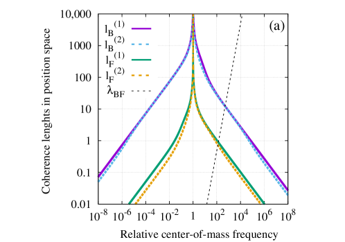
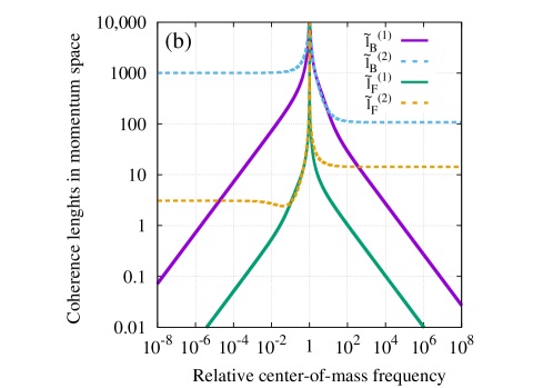
Figure 1: First-order and second-order dimensionless coherence lengths of the impurity and the condensate. The number of fermions is $N_{F}=2$ and the number of bosons $N_{B}=10,000$. The mass of a fermion is $m_{F}=1.0$ and that of a boson $m_{B}=0.01$. Panel (a) depicts the coherence lengths in position space and panel (b) in momentum space. The results are plotted against the relative center-of-mass frequency $\Omega_{BF}=\sqrt{\omega^{2}+2\left(\frac{N_{B}}{m_{F}}+\frac{N_{F}}{m_{B}}\right)\lambda_{BF}}$ [Eq. (2)] which satisfies $1<\Omega_{BF}$ for attractive and $0^{+}<\Omega_{BF}<1$ for repulsive interspecies interactions. For reference, in panel (a) the interspecies interaction strength $\lambda_{BF}=\frac{1}{2}\frac{m_{F}m_{B}}{M}\left(\Omega^{2}_{BF}-\omega^{2}\right)$ is plotted. The frequency of the trap is $\omega=1.0$. There are no intraspecies interactions, i.e., $\lambda_{F}=0$ and $\lambda_{B}=0$. Correlations build up only due to impurity-condensate interaction. The first-order coherence lengths in position and momentum spaces are equal whereas the second-order quantities can differ considerably. See the text for more details. The quantities shown are dimensionless.

4 Summary

A fermionic impurity embedded in a Bose-Einstein condensate is treated analytically, at the many-body level of theory, within the exactly-solvable harmonic-interaction model for trapped Bose-Fermi mixtures. In the present work, we have focused on the construction and analysis of correlation functions, both in position and momentum spaces, for $N_{F}=2$ fermions and a general number $N_{B}$ of bosons. For the fermionic impurity as well as for the condensate, we have prescribed the exact first-order and second-order correlation functions as functions of the masses $m_{F},m_{B}$ and intraspecies $\lambda_{F},\lambda_{B}$ and interspecies $\lambda_{BF}$ interaction strengths. Furthermore, we have studied properties of the various coherence lengths, defined as the ratio between the off-diagonal decay or growth length of a correlation function and the diagonal decay length of the respective (reduced) density. It has been found that the first-order coherence lengths in position and momentum spaces are equal, whereas the second-order quantities can differ significantly. Illustrative examples were presented and discussed. In particular, when the sole interaction is between the impurity and the condensate, all coherence lengths decay to zero for strong attraction or repulsion, except for the second-order coherence lengths in momentum space which saturate at finite values. As an obvious yet challenging outlook, it would be interesting to extend the Bose-Fermi harmonic-interaction model and its applications to time-dependent scenarios.

This research was supported by the Israel Science Foundation (Grant No. 1516/19).

Appendix A Limiting cases of the bosons’ and fermions’ first-order and second-order dimensionless coherence lengths in position and momentum spaces

Consider, first, the case of no interaction between the impurity and the condensate, i.e., $\Omega_{BF}=\omega$. We analyze the bosons but the results hold for the fermions as well. Then,

$$l_{B}^{(1)}=\tilde{l}_{B}^{(1)}=\frac{1}{\sqrt{\left[1+\frac{1}{N_{B}}\left(\frac{\omega}{\Omega_{B}}-1\right)\right]\left[1+\frac{1}{N_{B}}\left(\frac{\Omega_{B}}{\omega}-1\right)\right]-1}}\$$ (30)

and

$$\!\!\!\!\!\!\!\!\!\!\!\!\!\!\!\!l_{B}^{(2)}=\sqrt{\frac{1+\frac{1}{N_{B}}\left(\frac{\Omega_{B}}{\omega}-1\right)}{\left[1+\frac{2}{N_{B}}\left(\frac{\Omega_{B}}{\omega}-1\right)\right]\left|\frac{1}{N_{B}}\left(\frac{\Omega_{B}}{\omega}-1\right)\right|}},\quad\tilde{l}_{B}^{(2)}=\sqrt{\frac{1+\frac{1}{N_{B}}\left(\frac{\omega}{\Omega_{B}}-1\right)}{\left[1+\frac{2}{N_{B}}\left(\frac{\omega}{\Omega_{B}}-1\right)\right]\left|\frac{1}{N_{B}}\left(\frac{\omega}{\Omega_{B}}-1\right)\right|}}.$$

(31)

The limits $\lim_{\Omega_{B}\to\infty}$ and $\lim_{\Omega_{B}\to 0^{+}}$ of the coherence lengths (30) and (A) are all equal to zero expect for

$$\lim_{\Omega_{B}\to 0^{+}}l_{B}^{(2)}=\lim_{\Omega_{B}\to\infty}\tilde{l}_{B}^{(2)}=\sqrt{\frac{1-\frac{1}{N_{B}}}{\left(1-\frac{2}{N_{B}}\right)\frac{1}{N_{B}}}}.\$$ (32)

The meaning of (32) is that the second-order position and momentum coherence lengths are always finite (for a finite number of particles) at the limit of strong attractive and repulsive interactions, respectively, expect for a single pair of identical particles, $N_{B}=2$. Then, the coherence length diverges because the diagonal of the two-particle density is nothing but the pairs’ center-of-mass wavefunction (density) which does not depend on the interaction.

Next, consider the regime of parameters in which the interspecies interaction is ‘balanced’ by the intraspecies interactions, namely $\lambda_{F}=-\frac{N_{B}}{N_{F}}\lambda_{BF}$ and $\lambda_{B}=-\frac{N_{F}}{N_{B}}\lambda_{BF}$. Consequently, $\Omega_{F}=\Omega_{B}=\omega$. Furthermore, the energy (2) depends explicitly on the interspecies interaction only though the relative center-of-mass degree-of-freedom,

$$E=\frac{1}{2}\left[\left(N_{F}^{2}+N_{B}-1\right)\omega+\sqrt{\omega^{2}+2\left(\frac{N_{B}}{m_{F}}+\frac{N_{F}}{m_{B}}\right)\lambda_{BF}}\right].$$ (33)

Thus, we may call this regime of ‘balanced’ interactions the regime of ‘marginal interaction’, since only one out of $N_{F}+N_{B}$ degrees-of-freedom is explicitly interaction dependent. Now,

$$l_{B}^{(1)}=\tilde{l}_{B}^{(1)}=\frac{1}{\sqrt{\left[1+\frac{1}{N_{B}}\frac{m_{F}N_{F}}{M}\left(\frac{\Omega_{BF}}{\omega}-1\right)\right]\left[1+\frac{1}{N_{B}}\frac{m_{F}N_{F}}{M}\left(\frac{\omega}{\Omega_{BF}}-1\right)\right]-1}}\$$ (34)

and

$$l_{B}^{(2)}=\sqrt{\frac{1+\frac{1}{N_{B}}\frac{m_{F}N_{F}}{M}\left(\frac{\omega}{\Omega_{BF}}-1\right)}{\left[1+\frac{2}{N_{B}}\frac{m_{F}N_{F}}{M}\left(\frac{\omega}{\Omega_{BF}}-1\right)\right]\left|\frac{1}{N_{B}}\frac{m_{F}N_{F}}{M}\left(\frac{\omega}{\Omega_{BF}}-1\right)\right|}},$$

$$\tilde{l}_{B}^{(2)}=\sqrt{\frac{1+\frac{1}{N_{B}}\frac{m_{F}N_{F}}{M}\left(\frac{\Omega_{BF}}{\omega}-1\right)}{\left[1+\frac{2}{N_{B}}\frac{m_{F}N_{F}}{M}\left(\frac{\Omega_{BF}}{\omega}-1\right)\right]\left|\frac{1}{N_{B}}\frac{m_{F}N_{F}}{M}\left(\frac{\Omega_{BF}}{\omega}-1\right)\right|}}.\$$ (35)

The limits $\lim_{\Omega_{BF}\to\infty}$ and $\lim_{\Omega_{BF}\to 0^{+}}$ of the coherence lengths (34) and (A) are all equal to zero expect for

$$\lim_{\Omega_{BF}\to\infty}l_{B}^{(2)}=\lim_{\Omega_{BF}\to 0^{+}}\tilde{l}_{B}^{(2)}=\sqrt{\frac{1-\frac{1}{N_{B}}\frac{m_{F}N_{F}}{M}}{\left(1-\frac{2}{N_{B}}\frac{m_{F}N_{F}}{M}\right)\frac{1}{N_{B}}\frac{m_{F}N_{F}}{M}}},\$$ (36)

which are finite for any number of particles $N_{B}$ including a pair, compare to (32). The interspecies interaction dresses even a single pair of the other species, making the pair’s center-of-mass degree-of-freedom interaction dependent. Consequently, the respective second-order coherence lengths become finite at the limit of strong attractive and repulsive interactions, see (36).

Finally, equivalent limiting relations as the above, Eqs. (30-32) and (34-36), hold for the coherence lengths of the fermions, $l_{F}^{(1)}=\tilde{l}_{F}^{(1)}$, $l_{F}^{(2)}$, and $\tilde{l}_{F}^{(2)}$, with the obvious interchanges $N_{B}\Leftrightarrow N_{F}$, $\Omega_{B}\Leftrightarrow\Omega_{F}$, and $m_{F}\Leftrightarrow m_{B}$.

References

References

• [1] Bijlsma M J, Heringa B A and Stoof H T C 2000 Phys. Rev. A 61 053601
• [2] Lewenstein M, Santos L, Baranov M A and Fehrmann H 2004 Phys. Rev. Lett. 92 050401
• [3] Frahm H and Palacios G 2005 Phys. Rev. A 72 061604(R)
• [4] Imambekov A and Demler E 2006 Phys. Rev. A 73 021602(R)
• [5] Günter K, Stöferle T, Moritz H, Köhl M and Esslinger T 2006 Phys. Rev. Lett. 96 180402
• [6] Ospelkaus S, Ospelkaus C, Wille O, Succo M, Ernst P, Sengstock K and Bongs K 2006 Phys. Rev. Lett. 96 180403
• [7] Zaccanti M, D’Errico C, Ferlaino F, Roati G, Inguscio M and Modugno G 2006 Phys. Rev. A 74 041605(R)
• [8] Alon O E, Streltsov A I and Cederbaum L S 2007 Phys. Rev. A 76 062501
• [9] Girardeau M D and Minguzzi A 2007 Phys. Rev. Lett. 99 230402
• [10] Pollet L, Kollath C, Schollwöck U and Troyer M 2008 Phys. Rev. A 77 023608
• [11] Adhikari S K and Salasnich L 2008 Phys. Rev. A 78 043616
• [12] Fang B, Vignolo P, Gattobigio M, Miniatura C and Minguzzi A 2011 Phys. Rev. A 84 023626
• [13] Heinze J, Götze S, Krauser J S, Hundt B, Fläschner N, Lühmann D-S, Becker C and Sengstock K 2011 Phys. Rev. Lett. 107 135303
• [14] Wang H, Hao Y and Zhang Y 2012 Phys. Rev. A 85 053630
• [15] Yamamoto A and Hatsuda T 2012 Phys. Rev. A 86 043627
• [16] Bloom R S, Hu M-G, Cumby T D and Jin D S 2013 Phys. Rev. Lett. 111 105301
• [17] Wen L and Li J 2014 Phys. Rev. A 90 053621
• [18] Vaidya V D, Tiamsuphat J, Rolston S L and Porto J V 2015 Phys. Rev. A 92 043604
• [19] Bradlyn B and Andrey G 2016 Phys. Rev. A 93 033642
• [20] Cao L, Bolsinger V, Mistakidis S I, Koutentakis G M, Krönke S, Schurer J M and Schmelcher P 2017 J. Chem. Phys. 147 044106
• [21] DeSalvo B J, Patel K, Johansen J and Chin C 2017 Phys. Rev. Lett. 119 233401
• [22] Chen J, Schurer J M and Schmelcher P 2018 Phys. Rev. Lett. 121 043401
• [23] Trautmann A, Ilzhöfer P, Durastante G, Politi C, Sohmen M, Mark M J and Ferlaino F 2018 Phys. Rev. Lett. 121 213601
• [24] Kinnunen J J, Wu Z and Bruun G M 2018 Phys. Rev. Lett. 121 253402
• [25] Gautam S and Adhikari S K 2019 Phys. Rev. A 100 023626
• [26] Pasek M and Orso G 2019 Phys. Rev. B 100 245419
• [27] Sowiński T and García-March M Á 2019 Rep. Prog. Phys. 82 104401
• [28] Ye Z-X, Xie L-Y, Guo Z, Ma X-B, Wang G-R, You L and Tey M K 2020 Phys. Rev. A 102 033307
• [29] Jee K Y and Mueller E 2021 Phys. Rev. A 103 033307
• [30] Milczewski J von, Rose F and Schmidt R 2022 Phys. Rev. A 105 013317
• [31] Pâţu O I 2022 Phys. Rev. A 105 063309
• [32] Patel K, Cai G, Ando H and Chin C 2023 Phys. Rev. Lett. 131 083003
• [33] Pruski S, Maćkowiak J and Missuno O 1972 Rep. Math. Phys. 3 227
• [34] Robinson P D 1977 J. Chem. Phys. 66 3307
• [35] Hall R L 1978 J. Phys. A 11 1227
• [36] Cohen L and Lee C 1985 J. Math. Phys. 26 3105
• [37] Osadchii M S and Muraktanov V V 1991 Int. J. Quant. Chem. 39 173
• [38] Załuska-Kotur M A, Gajda M, Orłowski A and Mostowski J 2000 Phys. Rev. A 61 033613
• [39] Yan J 2003 J. Stat. Phys. 113 623
• [40] Gajda M 2006 Phys. Rev. A 73 023603
• [41] Zhao-Liang W, An-Min W, Yang Y and Xue-Chao L 2012 Commun. Theor. Phys. 58 639
• [42] Armstrong J R, Zinner N T, Fedorov D V and Jensen A S 2011 J. Phys. B 44 055303
• [43] Kościk P and Okopińska A 2013 Few-Body Syst. 54 1637
• [44] Schilling C 2013 Phys. Rev. A 88 042105
• [45] Bouvrie P A, Majtey A P, Tichy M C, Dehesa J S and Plastino A R 2014 Eur. Phys. J. D 68 346
• [46] Benavides-Riveros C L, Toranzo I V and Dehesa J S 2014 J. Phys. B 47 195503
• [47] Armstrong J R, Volosniev A G, Fedorov D V, Jensen A S and Zinner N T 2015 J. Phys. A 48 085301
• [48] Schilling C and Schilling R 2016 Phys. Rev. A 93 021601(R)
• [49] Klaiman S, Streltsov A I and Alon O E 2017 Chem. Phys. 482 362
• [50] Alon O E 2017 J. Phys. A 50 295002
• [51] Alon O E and Cederbaum L S 2023 J. Phys.: Conf. Ser. 2494 012014
• [52] Alon O E and Cederbaum L S 2023 arXiv:2311.08138v1 [cond-mat.quant-gas]
• [53] Lode A U J, Sakmann K, Alon O E, Cederbaum L S and Streltsov A I 2023 Phys. Rev. A 86 063606
• [54] Fasshauer E and Lode A U J 2016 Phys. Rev. A 93 033635
• [55] Lévêque C and Madsen L B 2018 J. Phys. B 51 155302
• [56] Lode A U J, Lévêque C, Madsen L B, Streltsov A I and Alon O E 2020 Rev. Mod. Phys. 92 011001
• [57] Bhowmik A and Alon O E 2023 arXiv:2309.05240v1 [cond-mat.quant-gas]
• [58] Alon O E and Cederbaum L S 2023 to be submitted
• [59] Löwdin P O 1955 Phys. Rev. 97 1474
• [60] Coleman A J and Yukalov V I 2000 Reduced Density Matrices: Coulson’s Challenge (Lectures Notes in Chemistry vol 72) (Berlin: Springer)
• [61] Glauber R J 1963 Phys. Rev. 130 2529
• [62] Naraschewski M and Glauber R J 1999 Phys. Rev. A 59 4595
• [63] Sakmann K, Streltsov A I, Alon O E and Cederbaum L S 2008 Phys. Rev. A 78 023615