cuPDLP.jl: A GPU Implementation of Restarted Primal-Dual Hybrid Gradient for Linear Programming in Julia

Abstract

In this paper, we provide an affirmative answer to the long-standing question: Are GPUs useful in solving linear programming? We present cuPDLP.jl, a GPU implementation of restarted primal-dual hybrid gradient (PDHG) for solving linear programming (LP). We show that this prototype implementation in Julia has comparable numerical performance on standard LP benchmark sets as Gurobi, a highly optimized implementation of the simplex and interior-point methods. Furthermore, we present the superior performance of cuPDLP.jl with its CPU counterpart. This demonstrates the power of using GPUs in the optimization solvers.

1 Introduction

Linear programming (LP) is a fundamental optimization problem class with a long history and a vast range of applications in operation research and computer science, such as agriculture, transportation, telecommunications, economics, production and operations scheduling, strategic decision-making, etc [28, 19, 16, 36, 14, 55].

Since the 1940s, speeding up and scaling up LP has been a central topic in the optimization community, with extensive studies from both academia and industry. The current general-purpose LP solvers, such as Gurobi [48], COPT [23], CPLEX [42] and HiGHS [31], are quite mature. These classic LP solvers are based on either the simplex method or interior-point methods (IPMs), which can generally provide high-quality solutions to LP. However, further scaling up or speeding up these methods is highly challenging. The fundamental difficulty is the necessity of solving linear systems in simplex and IPMs, which requires either LU factorization (for simplex method) or Cholesky factorization (for IPMs). Such factorization-based approaches have two major drawbacks when solving large instances: (i) Storing the factorization can be quite memory-demanding. It is often the case that a sparse matrix has a much denser factorization, which is one of the reasons for classic solvers to raise an “out-of-memory” error even if the instance can be stored in memory; (ii) Both methods are highly nontrivial to exploit massive parallelization, and thus they are infeasible to take advantage of modern computing architectures such as graphic processing units (GPUs) and distributed computing, due to the sequential nature of factorizations. Accordingly, all classic LP solvers are CPU-based and implemented on a single machine.

Nowadays, the scale of instances a classic LP solver can solve is rarely beyond 100 million variables. In contrast, the modern deep learning models used in practice, such as GPT-4, have trillions of variables. Notice that training a deep learning model, as a highly nonconvex optimization problem, is usually viewed as much harder than LP, which is perhaps the simplest non-trivial optimization problem. There is clearly a mismatch.

One commonly believed reason for the success of deep learning models is the extensive use of GPUs, which massively speeds up the neural network training process. Indeed, commercial solver companies, such as Gurobi, always try to use GPUs to speed up their solvers, but the previous efforts were unsuccessful [25, 26]. The fundamental reason is that GPUs do not work well for solving sparse linear systems, which is the computational bottleneck of simplex or barrier method solving linear programming [54, 25, 26].

This paper revisits this natural question:

Are GPUs useful in solving LP?

We provide an affirmative answer to this question by presenting cuPDLP.jl, a GPU implementation of restarted primal-dual hybrid gradient (PDHG) implemented in Julia. We present an extensive numerical study comparing cuPDLP.jl with its CPU counterpart and three methods implemented in the highly-optimized commercial LP solver Gurobi on standard LP benchmark sets, which showcase that

• cuPDLP.jl, a GPU implementation of PDLP in Julia programming language, has a comparable behavior with the highly-optimized commercial LP solver Gurobi on standard LP benchmark sets and has superior performance on large instances.

• Compared with its CPU counterpart, cuPDLP.jl clearly has superior performance and has more than ten times speed-up on at least one-third of the instances in standard benchmark sets. Furthermore, one can observe the strong correlation between the GPU speed-up and the size of the instances.

cuPDLP.jl can be viewed as a CUDA implementation of its CPU counterpart PDLP [3]. PDLP has two open-sourced implementations, a prototype implementation in Julia (FirstOrderLp.jl), and a production-level C++ implementation (open-sourced through Google OR-Tools).

Different from classic LP solvers, PDLP is a first-order method (FOM) LP solver. The fundamental difference is that the computational bottleneck of FOM is (sparse) matrix-vector multiplication, in contrast to (sparse) matrix factorization in simplex or IPMs. Table 1 presents a comparison summary of simplex, barrier, and FOM LP solvers in five different dimensions: cost per iteration, number of iterations needed to solve an instance, code complexity, whether they can take advantage of massive parallelization, and whether they need extensive memory usage (beyond just storing the instance itself). As we can see, FOMs have multiple advantages in solving large instances, compared with simplex and IPMs.

In particular, thanks to the recent development of deep learning, (sparse) matrix-vector multiplication suits very well on modern GPU infrastructure. Additionally, it is also shown that PDLP has strong theoretical guarantees [5, 4, 37, 39] and superior numerical performance compared to other FOM-based solvers [3]. These are the reasons we choose PDLP as the base algorithm in our GPU implementation.

To fully unleash the potential offered by modern GPU hardware, there are a few differences and modifications to the original CPU-based PDLP: (1) Due to the slow communication between CPU and GPU, the computational framework of PDLP has to be fully implemented on GPUs. In other words, both the instances and intermediate iterates of GPU must be resident within GPU memory (see Section 3.2 for details); (2) A key enhancement adopted by PDLP, namely adaptive restart with respect to normalized duality gap, cannot be efficiently evaluated on GPU, and we replace it by a KKT gap based adaptive restarting scheme (see Section 3.4 for details).

As a side contribution, we provide a coding framework and example of developing a high-performance FOM-based optimization solver on GPUs in Julia programming language, which we believe is of independent interest to the computational optimization community.

Table 1: Comparison of simplex, barrier, and first-order methods in five dimensions, where green, gray, and red faces represent a decreasing order of favorableness of the corresponding method in the corresponding dimension.

1.1 Related literature

Linear programming and classic solvers. Linear programming (LP) is one of the most fundamental tools in operation research and computer science, with wide practical applications [2, 9, 10, 17, 13, 27, 36, 41]. Since the 1940s, speeding up and scaling up LP has been a central topic in the optimization community, with extensive studies in both academia and industry. The state-of-the-art methods to solve LP are simplex methods[18] and interior-point methods [32]. Based on these methods, commercial solvers such as Gurobi [48] and COPT [23] and open-sourced solvers like HiGHS [31] can provide reliable solutions with high accuracy.

FOM-based LP solvers. There is a recent surge of research on using first-order methods (FOMs) to solve linear programming. FOMs are appealing due to their low per-iteration cost and ability of parallelization.

• PDHG-based solvers: PDLP [3]. PDLP is a general-purpose large-scale LP solver. PDLP is built upon restarted PDHG algorithm [5], with many practical algorithmic enhancements, such as preconditioning, adaptive restart, adaptive step-size, infeasibility detection, etc. Currently PDLP has three implementations: a prototype implemented in Julia (FirstOrderLp.jl), a production-level C++ implementation (open-sourced through Google OR-Tools), and an internal distributed version at Google [43]. There is also an extensive study on the theoretical results related to PDLP, such as, the linear convergence rate [37, 5], infeasibility detection [4], refined complexity analysis [39, 30], extensions to quadratic programming [40], etc.

• Matrix-free IPM solvers: ABIP [35, 20]. The core algorithm of ABIP is solving the homogeneous self-dual embedded cone programs via an interior-point method, and as a special case, it can solve LP. ABIP utilizes multiple ADMM iterations instead of one Newton step to approximately minimize the log-barrier penalty function. A recently enhanced version of ABIP (named ABIP+ [20]) includes many new enhancements, such as preconditioning, restart, and hybrid parameter tuning, on top of ABIP. It was shown that ABIP+ (developed in C) has a comparable numerical performance on the LP benchmark sets to the Julia implementation of PDLP.

• Dual-based solvers: ECLIPSE [6]. ECLIPSE is a distributed LP solver. It leverages accelerated gradient descent to solve a smoothed dual form of LP. ECLIPSE is designed specifically to solve large-scale LPs with certain decomposition structures arising from web applications. For example, ECLIPSE is used to solve real-world web applications with $10^{12}$ decision variables at LinkedIn [51, 1].

• ADMM-based solvers: SCS [47, 46]. SCS is designed to solve large-scale convex cone programs. It tackles the homogeneous self-dual embedding of general conic programming using ADMM. LP is solved as a special case of cone programming in SCS. The computational bottleneck of ADMM-based methods is solving a linear system with similar forms every iteration. SCS supports using direct solve or indirect solve via the conjugate gradient method. The first approach still requires doing a factorization and thus suffers from the same scaling difficulties as simplex and IPMs. The second approach usually requires at least 20 conjugate gradient steps (i.e., matrix-vector multiplications) for every iteration and is not competitive compared with the PDHG-based algorithms as shown in [3].

Primal-dual hybrid gradient method (PDHG). PDHG is an operator splitting method initially designed for applications in image processing [11, 15, 21, 29, 56]. PDHG exhibits a sub-linear rate on general convex-concave problems [12, 38] and achieves linear rate on a wide class of problems [37, 22]. PDLP [3] utilizes PDHG as its base algorithm. Built on the ergodic convergence of PDHG, a restart variant of PDHG exhibits an optimal linear convergence rate for solving LP [5]. [4] shows how to extract infeasibility information of LP from PDHG iterates.

Optimization with GPUs. To the best of our knowledge, there does not exist any general-purpose LP solvers on GPUs. Previous efforts to solve LP on GPUs have not yet been successful due to the inefficiency of solving linear systems on GPUs [25, 26, 54]. Despite this, a few works use GPUs to solve nonlinear programming with applications in power systems [34, 33, 49, 53].

2 PDLP

In this section, we introduce the basics of LP and the algorithmic components of PDLP, as stated in [3]. After a brief introduction of vanilla PDHG for solving LP (Section 2.1), we summarize the enhancements of PDLP on top of PDHG that boost the practical performance (Section 2.2).

Consider LP of the general form:

$$\min_{x\in\mathbb{R}^{n}}{}{} ~{}c^{\top}x$$ (1)

s.t. $$~{}Gx\geq h$$

$$~{}Ax=b$$

$$~{}l\leq x\leq u\ ,$$

where $G\in\mathbb{R}^{m_{1}\times n}$, $A\in\mathbb{R}^{m_{2}\times n}$, $c\in\mathbb{R}^{n}$, $h\in\mathbb{R}^{m_{1}}$, $b\in\mathbb{R}^{m_{2}}$, $l\in(\mathbb{R}\cup\{-\infty\})^{n}$, $u\in(\mathbb{R}\cup\{\infty\})^{n}$. Notice that the constraint set is a complicated polytope that is hard to be projected onto, which makes it intractable to use standard FOMs, such as, projected gradient descent for solving (1). PDLP solves the primal-dual form of the problem by dualizing the linear constraints:

$$\min_{x\in X}\max_{y\in Y}\ L(x,y):=c^{\top}x-y^{\top}Kx+q^{\top}y\ ,$$ (2)

where $K^{\top}=\begin{pmatrix}G^{\top},A^{\top}\end{pmatrix}$ and $q^{\top}:=\begin{pmatrix}h^{\top},b^{\top}\end{pmatrix}$, $X:=\{x\in\mathbb{R}^{n}:l\leq x\leq u\}$, and $Y:=\{y\in\mathbb{R}^{m_{1}+m_{2}}:y_{1:m_{1}}\geq 0\}.$ By duality theory, it is straightforward to show that a saddle point of (2) recovers an optimal primal-dual solution to (1).

2.1 PDHG for solving LP

The base algorithm of PDLP is the primal-dual hybrid gradient (PDHG, a.k.a. Chambolle-Pock method) [11]. The update of PDHG for solving (2) is

$$\begin{cases}x^{t+1}\leftarrow\text{proj}_{X}(x^{t}-\tau(c-K^{\top}y^{t}))\\ y^{t+1}\leftarrow\text{proj}_{Y}(y^{t}+\sigma(q-K(2x^{t+1}-x^{t})))\ ,\end{cases}$$ (3)

where $\tau,\sigma$ are primal and dual step-sizes respectively. The computational bottleneck of PDHG is matrix-vector multiplication $K^{\top}y^{t}$ and $Kx^{t}$; thus, PDHG is fully matrix-free to solve LP, i.e., it does not need to solve any linear equations. The primal and the dual step-size are reparameterized in PDLP as

$$\tau=\eta/\omega,\;\sigma=\eta\omega\quad\text{with}\;\ \eta,\omega>0\ ,$$

where $\eta$ (called step-size) controls the scale of the step-sizes, and $\omega$ (called primal weight) balances the primal and the dual progress.

2.2 Algorithmic enhancements in PDLP

We here summarise the algorithmic enhancements in PDLP that is presented in [3]. It turns out that the numerical performance of vanilla PDHG (3) on LP is not strong enough to support a modern solver [3]. To boost the practical performance, PDLP has essentially five major enhancements on top of PDHG: preconditioning, adaptive restart, adaptive step-size, primal weight update, and infeasibility detection. The core algorithm in PDLP, i.e., restarted PDHG, is presented in Algorithm 1, followed by discussions on each algorithmic enhancement adopted.

Input : Initial point $z^{0,0}$;

1 Initialize outer loop counter $n\leftarrow 0$, total iterations $k\leftarrow 0$, step-size $\hat{\eta}^{0,0}\leftarrow 1/\|K\|_{\infty}$, primal weight $\omega^{0}\leftarrow\text{InitializePrimalWeight}(c,q)$;

2 repeat

3       $t\leftarrow 0$;

4       repeat

5             $z^{n,t+1},\eta^{n,t+1},\hat{\eta}^{n,t+1}\leftarrow\text{AdaptiveStepPDHG}(z^{n,t},\omega^{n},\hat{\eta}^{n,t},k)$;

6             $\bar{z}^{n,t+1}\leftarrow\tfrac{1}{\sum_{i=1}^{t+1}\eta^{n,i}}\sum_{i=1}^{k+1}\eta^{n,i}z^{n,i}$;

7             $z_{c}^{n,t+1}\leftarrow\text{GetRestartCandidate}(z^{n,t+1},\bar{z}^{n,t+1})$;

8             $t\leftarrow t+1$, $k\leftarrow k+1$;

9            

10      until restart or termination criteria holds;

11      restart the outer loop $z^{n+1,0}\leftarrow z_{c}^{n,t}$, $n\leftarrow n+1$;

12       $\omega^{n}\leftarrow\text{PrimalWeightUpdate}(z^{n,0},z^{n-1,0},\omega^{n-1})$;

13      

14until termination criteria holds;

Output : $z^{n,0}$.

Algorithm 1 Restarted PDHG (after preconditioning)

• Preconditioning: The efficacy of first-order methods is closely tied to the conditioning of the underlying problem. In order to mitigate the ill-posedness, PDLP employs a diagonal preconditioner to ameliorate the condition number of the original problem. Specifically, it involves the rescaling of the constraint matrix $K=(G,A)$ to $\tilde{K}=(\tilde{G},\tilde{A})=D_{1}KD_{2}$ where $D_{1}$ and $D_{2}$ are positive diagonal matrices. This rescaling ensures that the resulting matrix $\tilde{K}$ is ”well balanced”. Consequently, this preconditioning step gives rise to a modified LP instance, wherein $A,G,c,b,h,u$ and $l$ in (1) are replaced with $\tilde{G},\tilde{A},\hat{x}=D_{2}^{-1}x,\tilde{c}=D_{2}c,(\tilde{b},\tilde{h})=D_{1}(b,h),\tilde{u}=D_{2}^{-1}u$ and $\tilde{l}=D_{2}^{-1}l$. In the default PDLP configuration, a combination of Ruiz rescaling [52] and the preconditioning technique proposed by Pock and Chambolle [50] is employed.

• Adaptive restarts. PDLP utilizes an adaptive restarting strategy to enhance convergence. PDLP initially selects a restart candidate at each iteration, choosing between the current iterate and the average iterate based on a greedy principle. Subsequently, various restart criteria are assessed to determine if there is a constant factor decay in the progress metric. If such decay is observed, a restart is triggered. Further details can be found in [5].

  In the CPU-based PDLP, the progress metric for restarting is the normalized duality gap proposed in [5], and a trust-region algorithm is devised to compute this metric efficiently. While the trust-region algorithm exhibits linear time complexity, it is less compatible with GPUs’ massively parallel computing paradigm. Therefore, in cuPDLP.jl, we introduce a novel restart scheme based on the KKT error. Detailed discussions are deferred to Section 3.4.

• Adaptive step-size. The step-size suggested by theoretical considerations, namely $1/\|A\|_{2}$, turns out to be conservative in practical applications. To address this, PDLP employs a heuristic line search to determine a suitable step-size satisfying the condition:

  $$\eta\leq\frac{\|z^{t+1}-z^{t}\|_{\omega}^{2}}{2(y^{t+1}-y^{t})^{\top}K(x^{t+1}-x^{t})}\ ,$$ (4)

  where $\|z\|_{\omega}:=\sqrt{\omega\|x\|_{2}^{2}+\frac{\|y\|_{2}^{2}}{\omega}}$ and $\omega$ is the current primal weight. Additional details of the adaptive step-size rule are elaborated in [3]. The inequality (4) was inspired from the $\mathcal{O}(1/k)$ convergence rate proof of PDHG [12, 38]. The empirical evidence from numerical experiments conducted in [3] attests to its consistent efficacy.

  Function : AdaptiveStepPDHG($z^{n,t}$, $\omega^{n}$, $\hat{\eta}^{n,t}$,$k$)

  1

  2$(x,y)\leftarrow z^{n,t}$, $\eta\leftarrow\hat{\eta}^{n,t}$

  3 for $i=0,1,...$ do

  4       $x^{\prime}\leftarrow\mathrm{proj}_{X}(x-\frac{\eta}{\omega^{n}}(c-K^{\top}y))$

  5       $y^{\prime}\leftarrow\mathrm{proj}_{Y}(y+{\eta}{\omega^{n}}(q-K(2x^{\prime}-x)))$

  6       $\bar{\eta}\leftarrow\frac{\|(x^{\prime}-x,y^{\prime}-y)\|_{\omega^{n}}^{2}}{2(y^{\prime}-y)^{\top}K(x^{\prime}-x)}$

  7       $\eta^{\prime}\leftarrow\min\left({(1-(k+1)^{-0.3})\bar{\eta},(1+(k+1)^{-0.6})\eta}\right)$

  8       if $\eta\leq\bar{\eta}$ then

  9             return $(x^{\prime},y^{\prime})$, $\eta$, $\eta^{\prime}$

  10       end if

  11      $\eta\leftarrow\eta^{\prime}$

  12 end for

  Algorithm 2 One step of PDHG using adaptive step-size heuristic

• Primal Weight Update: Adjusting the primal weight $\omega$ is designed to harmonize the primal and dual spaces through a heuristic approach. The update of primal weight is specific during restart occurrences, thus infrequently. More precisely, the initialization of $\omega$ involves the expression:

  $$\mathrm{InitializePrimalWeight}(c,q):=\begin{cases}\frac{\|c\|_{2}}{\|q\|_{2}},\;&\text{if }\|c\|_{2},\|q\|_{2}>\epsilon_{\mathrm{zero}}\\ 1,\;&\mathrm{otherwise}\end{cases}$$

  where $\epsilon_{\mathrm{zero}}$ denotes a small nonzero tolerance. Let $\Delta_{x}^{n}=\|x^{n,0}-x^{n-1,0}\|_{2}$ and $\Delta_{y}^{n}=\|y^{n,0}-y^{n-1,0}\|_{2}$. PDLP initiates the primal weight update at the beginning of each new epoch.

  $$\mathrm{PrimalWeightUpdate}(z^{n,0},z^{n-1,0},\omega^{n-1}):=\begin{cases}\exp\left({\theta\log\left({\frac{\Delta_{y}^{n}}{\Delta_{x}^{n}}}\right)+(1-\theta)\omega^{n-1}}\right),\;&\Delta_{x}^{n},\Delta_{y}^{n}>\epsilon_{\mathrm{zero}}\\ \omega^{n-1},\;&\mathrm{otherwise}\end{cases}$$

  The intuition is to determine the primal weight $\omega^{n}$ in a manner that equalizes the distance to optimality in both the primal and dual domains, i.e., $\|(x^{n,t}-x^{*},0)\|_{\omega^{n}}\approx\|(0,y^{n,t}-y^{*})\|_{\omega^{n}}$. Additionally, PDLP employs exponential smoothing with a parameter $\theta\in[0,1]$ to mitigate oscillations.

• Infeasibility detection. PDLP periodically checks whether the difference of iterates $z^{n,t+1}-z^{n,t}$ or the normalized iterates $\frac{1}{t}(z^{n,t}-z^{n,0})$ provide an infeasibility certificate, and the performance of these two sequences is instance-dependent. A detailed investigation of infeasibility detection using PDHG iterates is available in [4].

3 GPU implementation of PDLP

This section presents the design of cuPDLP.jl, the GPU implementation of PDLP. Section 3.1 briefly introduces the hardware architecture and logical structure. In Section 3.2, we discuss in detail the design of cuPDLP.jl. Section 3.3 presents the implementation of basic matrix and vector operations in cuPDLP.jl, and Section 3.4 shows the restart scheme based on KKT error to adapt on GPU. The solver is available at https://github.com/jinwen-yang/cuPDLP.jl.

3.1 GPU architecture and thread hierarchy

GPUs exhibit distinct underlying architecture with CPUs. GPUs have significantly more computation cores than CPUs. For example, the GPU we used in the experiments, NVIDIA Tesla V100, has 2688 double-precision cores. However, unlike CPU cores, many GPU cores share the same control unit and must execute the same instruction simultaneously. As a result, the hardware design of GPUs encourages high bandwidth instead of a deep pipeline.

GPUs follow the single instruction multiple data (SIMD) computational paradigm; namely, the threads execute the same instruction but fetch their own data. At the heart of GPU programming is the kernel function, i.e., a program designed to execute instructions on GPUs. Upon launching the kernel function, the execution environment configures a grid of thread blocks, each block comprising an identical number of threads. A block of threads is assigned to an available streaming multiprocessor (SM) during runtime, directing them into warps, with each warp typically encompassing a set of 32 threads. Warp is the basic unit of execution in GPUs. One caveat goes that this does not mean that all thread blocks can run concurrently on SMs, and there are no guarantees on the order of block and warp execution.

This hierarchical structure is the backbone of GPUs to foster parallel execution across threads, optimizing computational efficiency. The relationship between the physical architecture and logical structure is depicted in Figure 1. For more detailed discussion in the characteristic of GPUs, refer to [45].

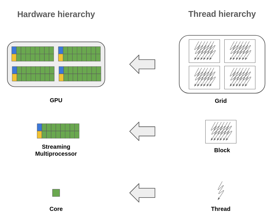
Figure 1: Illustration of the relationship between physical architecture and logical structure.

Each GPU device has its own memory hardware, which is separate from the memory of the CPU host. A typical computational paradigm is using CPUs for IO process and exploiting GPUs for burdensome computation. Thus, data moving between CPU and GPU are needed. However, the significant cost of CPU-GPU communication, especially for large-scale problems, can be a crucial issue. Frequent data transfers between CPU and GPU can introduce dominating communication cost over any computational speed-up gained on GPU.

3.2 Design of cuPDLP.jl

The design of cuPDLP.jl is illustrated in Figure 2. To avoid expensive data transfers between CPU and GPU, we have designed our implementation of cuPDLP.jl to run as much as possible on the GPU. In particular, Table 2 lists the computational components of CPU and GPU.

CPU		GPU
•  Input & Output •  Preconditioning		•  Main update of PDHG •  Adaptive restart •  Adaptive step-size •  Primal weight update •  Infeasibility detection •  Evaluate progress metric

Table 2: Computational modules on CPU and GPU.

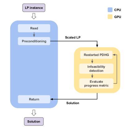
Figure 2: Illustration of the computational architecture of cuPDLP.jl.

As depicted in Figure 2, only two communications between CPU and GPU are required for cuPDLP.jl. One transfers the scaled LP instance after preconditioning from CPU to GPU while the other moves the final solution from GPU to CPU as output. Major iterations are executed completely on GPU and there is no need to transfer any vectors before termination to alleviate expensive CPU-GPU communication.

3.3 Vector and matrix operations

Matrix-vector multiplications and vector-vector operations, the core of PDLP, can be parallelized naturally and fit well with the SIMD paradigm of GPUs. GPUs have massive parallelization capability to manipulate each coordinate of vectors on each of its core in a parallel fashion. Specifically, the constraint matrix is stored in Compressed Sparse Row (CSR) format and cuPDLP.jl uses the 1-dimensional thread configuration since most of our operations are matrix-vector and vector-vector operations. We write our custom kernels for main PDHG updates (3) in cuPDLP.jl and utilize cusparseSpMV() implemented in cuSPARSE library to do matrix-vector multiplications. In our customized kernel, each thread updates a single coordinate of the iterate vector to maximize the throughput and cusparseSpMV() uses algorithm CUSPARSE_SPMV_CSR_ALG2 to provide a deterministic result for each run.

3.4 Adaptive restart based on KKT error

PDLP utilizes normalized duality gap as the progress metric for restart, which was introduced in [5]. The normalized duality gap for LP is computed by a trust-region algorithm. Although only linear time is needed, it is highly nontrivial to implement the trust-region method in an efficient parallel version on GPU. We use the KKT error defined in (5) as a proxy to the normalized duality gap for restarting since KKT error can be evaluated very efficiently on GPU.

$$\mathrm{KKT}_{\omega}(z)=\sqrt{\omega^{2}\left\|\begin{pmatrix}Ax-b\\ [h-Gx]^{+}\end{pmatrix}\right\|_{2}^{2}+\frac{1}{\omega^{2}}\|c-K^{\top}y-\lambda\|_{2}^{2}+(q^{\top}y+l^{\top}\lambda^{+}-u^{\top}\lambda^{-}-c^{\top}x)^{2}}$$ (5)

More specifically, the restart scheme is described as follows

Choosing the restart candidate.

$$z_{c}^{n,t+1}:=\mathrm{GetRestartCandidate}(z^{n,t+1},\bar{z}^{n,t+1})=\begin{cases}z^{n,t+1},&\mathrm{KKT}_{\omega^{n}}(z^{n,t+1})<\mathrm{KKT}_{\omega^{n}}(\bar{z}^{n,t+1})\\ \bar{z}^{n,t+1},&\mathrm{otherwise}\ .\end{cases}$$

Restart criteria. Define parameters $\beta_{\mathrm{sufficient}}=0.2$, $\beta_{\mathrm{necessary}}=0.8$ and $\beta_{\mathrm{artificial}}=0.36$. Denote $k$ the total iteration counter. The algorithm restarts if one of three conditions holds:

1. (Sufficient decay in KKT error)

   $$\mathrm{KKT}_{\omega^{n}}(z_{c}^{n,t+1})\leq\beta_{\mathrm{sufficient}}\mathrm{KKT}_{\omega^{n}}(z^{n,0})\ ,$$

2. (Necessary decay + no local progress in KKT error)

   $$\mathrm{KKT}_{\omega^{n}}(z_{c}^{n,t+1})\leq\beta_{\mathrm{necessary}}\mathrm{KKT}_{\omega^{n}}(z^{n,0})\quad\text{and}\quad\mathrm{KKT}_{\omega^{n}}(z_{c}^{n,t+1})>\mathrm{KKT}_{\omega^{n}}(z_{c}^{n,t})\ ,$$

3. (Long inner loop)

   $$t\geq\beta_{\mathrm{artificial}}k\ .$$

4 Numerical experiments

In this section, we study the numerical performance of cuPDLP.jl. In particular, we compare cuPDLP.jl with the CPU implementations of PDLP [3] and three methods implemented in the commercial solver Gurobi [48], i.e., primal simplex method, dual simplex method, and interior-point method. Section 4.1 describes the setup of the experiments. Section 4.2 presents the numerical results on LP relaxations of instances from MIPLIB 2017 collection [24]. More specifically, Section 4.2.1 investigates the performance of cuPDLP.jl and Gurobi, and Section 4.2.2 compares cuPDLP.jl with different versions of PDLP, namely Julia implemented FirstOrderLp.jl and C++ implemented PDLP with single thread and multiple threads. Section 4.3 discusses the performances of different solvers on Mittelmann’s LP benchmark set [44].

4.1 Experimental setup

Benchmark datasets. We use two LP benchmark datasets in the numerical experiments, MIP Relaxations, which contain 383 instances curated from root-node LP relaxation of mixed-integer programming problems from MIPLIB 2017 collection [24] (see Section 4.2), and 49 LP instances from the Mittelmann’s LP benchmark dataset [44] (see Section 4.3).

In particular, MIPLIB 2017 [24] is a collection of mixed-integer linear programming problems. We utilize the root-node LP relaxation of instances in MIPLIB as the LP benchmark set. 383 instances are selected from MIPLIB 2017 to construct MIP Relaxations based on the following criteria (similar selection criteria are used in the experiments of CPU-based PDLP [3]):

• Not tagged as numerically unstable

• Not tagged as infeasible

• Not tagged as having indicator constraints

• Finite optimal objective (if known)

• The constraint matrix has a number of nonzeros greater than 100,000

• Zero is not the optimal solution to the LP relaxation.

MIP Relaxations is further split into three classes based on the number of nonzeros (nnz) in the constraint matrix, as shown in Table 3.

	Small	Medium	Large
Number of nonzeros	100K - 1M	1M - 10M	>10M
Number of instances	269	94	20

Table 3: Scales of instances in MIP Relaxations

Mittelmann’s LP is a classic dataset to benchmark LP solvers. We utilize the 49 public instances from the dataset. The number of nonzeros of the instances spans from 100 thousand to 90 million.

Software. cuPDLP.jl is implemented in an open-source Julia [8] module. cuPDLP.jl utilizes CUDA.jl [7] as the interface for working with NVIDIA CUDA GPUs using Julia. We compare cuPDLP.jl with five LP solvers: the Julia implementation of PDLP (FirstOrderLp.jl), the C++ implementation of PDLP with single thread and multiple threads (wrapped in Google OR-Tools), the primal simplex, dual simplex and barrier method implemented in Gurobi. Crossover is disabled, and single-threaded is used in experiments of the Gurobi barrier. The running time of cuPDLP.jl and FirstOrderLp.jl is measured after pre-compilation in Julia.

Computing environment. We utilize UChicago Midway3 cluster in our experiments. More specifically, we use NVIDIA Tesla V100-PCIe-16GB GPU, with CUDA 11.5, for running cuPDLP.jl, and we use Intel Xeon Gold 6248R CPU 3.00GHz with 16GB RAM for running CPU-based solvers. The experiments are performed in Julia 1.9.0 and Gurobi 9.1 . Table 4 compares the theoretical peak of double-precision FLOPS (floating-point operations per second) of the CPU and GPU used in the experiments.

	CPU (single thread)	GPU
Processor	Intel Xeon Gold 6248R CPU 3.00GHz	NVIDIA Tesla V100-PCIe-16GB
Theoretical peak (FP64)	48 GFLOPS	7 TFLOPS
Maximum memory bandwidth	131.13 GB/sec	900 GB/sec

Table 4: Comparison of CPU and GPU specifications.

Initialization. Both PDLP and cuPDLP.jl uses all-zero vectors as the initial starting points.

Optimality termination criteria. PDLP and cuPDLP.jl terminate when the relative KKT error is no greater than the termination tolerance $\epsilon\in(0,\infty)$:

$$|q^{\top}y+l^{\top}\lambda^{+}-u^{\top}\lambda^{-}-c^{\top}x| \leq\epsilon(1+|q^{\top}y+l^{\top}\lambda^{+}-u^{\top}\lambda^{-}|+|c^{\top}x|)$$

$$\left\|\begin{pmatrix}Ax-b\\ [h-Gx]^{+}\end{pmatrix}\right\|_{2} \leq\epsilon(1+\|q\|_{2})$$

$$\|c-K^{\top}y-\lambda\|_{2} \leq\epsilon(1+\|c\|_{2})\ .$$

We use $\epsilon=10^{-4}$ for moderately accurate solutions and $\epsilon=10^{-8}$ for high-quality solutions. We also set $10^{-4}$ and $10^{-8}$ tolerances for parameters FeasibilityTol, OptimalityTol and BarConvTol (for barrier methods) of Gurobi.

Time limit. In Section 4.2, we impose a time limit of 3600 seconds on instances with small-sized and medium-sized instances and a time limit of 18000 seconds for large instances. For Section 4.3, we impose 15000 seconds as the time limit as in Mittelmann’s benchmark [44].

Shifted geometric mean. We report the shifted geometric mean of solve time to measure the performance of solvers on a certain collection of problems. More precisely, shifted geometric mean is defined as $\left(\prod_{i=1}^{n}(t_{i}+\Delta)\right)^{1/n}-\Delta$ where $t_{i}$ is the solve time for the $i$-th instance. We shift by $\Delta=10$ and denote it SGM10. If the instance is unsolved, the solve time is always set to the corresponding time limit.

4.2 MIP Relaxations

In this section, we compare cuPDLP.jl with the commercial LP solver Gurobi and CPU implementations of PDLP on MIP Relaxations respectively. The main message is that GPU-implemented cuPDLP.jl exhibits significant speedup over its CPU-implemented counterparts, and its numerical performance is on par with Gurobi.

4.2.1 cuPDLP.jl versus Gurobi

	Small (269) (1-hour limit)		Medium (94) (1-hour limit)		Large (20) (5-hour limit)		Total (383)
	Count	Time	Count	Time	Count	Time	Count	Time
cuPDLP.jl	265	10.91	89	17.60	18	156.80	372	14.94
Primal simplex (Gurobi)	268	7.81	73	140.18	13	1180.42	354	27.44
Dual simplex (Gurobi)	267	5.75	87	45.49	13	973.96	367	16.62
Barrier (Gurobi)	268	2.91	86	37.95	13	576.57	367	11.74

Table 5: Solve time in seconds and SGM10 of different solvers on instances of MIP Relaxations with tolerance $10^{-4}$: cuPDLP.jl versus Gurobi.

	Small (269) (1-hour limit)		Medium (94) (1-hour limit)		Large (20) (5-hour limit)		Total (383)
	Count	Time	Count	Time	Count	Time	Count	Time
cuPDLP.jl	257	30.17	89	52.50	16	434.34	362	40.76
Primal simplex (Gurobi)	266	9.06	68	166.03	12	1578.04	346	31.44
Dual simplex (Gurobi)	265	7.14	84	60.97	11	1438.33	360	20.63
Barrier (Gurobi)	268	3.38	82	46.13	13	630.21	363	13.28

Table 6: Solve time in seconds and SGM10 of different solvers on instances of MIP Relaxations with tolerance $10^{-8}$: cuPDLP.jl versus Gurobi.

Table 5 and Table 6 present a comparison between cuPDLP.jl and the commercial LP solver Gurobi, yielding several noteworthy observations:

• In the case of moderate accuracy ($\epsilon=10^{-4}$), cuPDLP.jl exhibits comparable performance to Gurobi regarding solved count and solve time. For medium-sized and large-sized instances, cuPDLP.jl establishes an advantage over Gurobi, achieving a 2x speed-up on medium problems with 3 more instances solved and a 3.7x speed-up on large instances with 5 additional solved instances, respectively.

• When seeking high-accuracy solutions, while Gurobi has advantages for small instances, cuPDLP.jl demonstrates comparable runtime to the best of the three Gurobi methods (i.e., barrier method) on medium-scale instances and a 1.5x speed-up on large-scale instances. In terms of solved count, cuPDLP.jl solves 7 more instances on medium scale and 3 more on large scale compared with Gurobi’s barrier algorithm, the best of the three in performance.

To summarize, these observations affirm that cuPDLP.jl attains comparable performance to Gurobi in MIP Relaxations benchmark dataset and exhibits superior performance on larger instances. This demonstrates that a first-order-method-based LP solver on GPU can be on par with a strong implementation of simplex and barrier methods, even in obtaining high-accuracy solutions.

Figure 3 shows the number of solved instances of cuPDLP.jl and three methods in Gurobi on MIP Relaxations in a given time. The y-axes display the fraction of solved instances, and the x-axes display the wall-clock time in seconds. As shown in the left panel, when seeking solutions with moderate accuracy ($\epsilon=10^{-4}$), cuPDLP.jl has comparable performances with Gurobi barrier after 10 seconds. It eventually has better performances on MIP Relaxation than all three methods of Gurobi. In addition, we can see the performance of cuPDLP.jl for high-quality solution ($\epsilon=10^{-8}$), as shown in the right panel, is still comparable to Gurobi. An observation is that the number of instances Gurobi can solve for a given running time does not differ much for moderate and high accuracy; conversely, such difference is more apparent for cuPDLP.jl. This is a feature of a first-order-method-based solver. Another interesting fact is that Gurobi solves about 40% of instances within one second, which is exactly the power of Gurobi. On the other hand, cuPDLP.jl has a computational overhead of around one second due to the GPU kernel launch time.

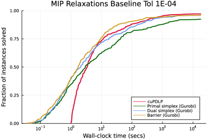
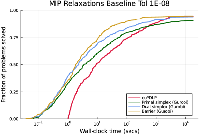
Figure 3: Number of instances solved for MIP Relaxations under moderate accuracy (left) and high accuracy (right): cuPDLP.jl versus Gurobi.

Notice that the GPU implementation of PDLP is motivated to solve larger and harder instances. Here, we further refine the selection of instances in the MIP Relaxations dataset by excluding those simple instances that at least one of the three Gurobi methods can solve within one second, a duration approximately equivalent to the kernel launch time for cuPDLP.jl. The outcomes are summarized in Table 7. Here are a few observations:

• For moderate accuracy, cuPDLP.jl successfully solves 188 instances out of a total of 196, surpassing Gurobi barrier and dual simplex by 8 instances and outperforming Gurobi primal simplex by 21 instances. Additionally, in terms of solve time, cuPDLP.jl exhibits faster performance compared to all three Gurobi methods. Particularly noteworthy is the observation that cuPDLP.jl achieves a 2x speed-up over Gurobi dual simplex and a 4x speed-up over Gurobi primal simplex.

• In the pursuit of high-quality solutions with $\epsilon=10^{-8}$, cuPDLP.jl continues to excel by solving the highest number of instances while maintaining comparable solve times to Gurobi dual simplex.

	Tol 1E-04 (196)		Tol 1E-08 (204)
	Count	Time	Count	Time
cuPDLP.jl	188	25.33	188	77.29
Primal simplex (Gurobi)	167	96.55	167	113.69
Dual simplex (Gurobi)	180	49.18	181	62.62
Barrier (Gurobi)	180	32.03	184	34.67

Table 7: Performances on MIP Relaxations instances that cannot be solved within 1 second by Gurobi. 196 instances for moderate accuracy $\epsilon=10^{-4}$ and 204 instances for high accuracy $\epsilon=10^{-8}$. Solve time in seconds and SGM10 is reported.

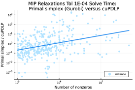
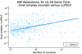
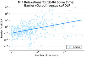
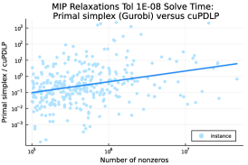
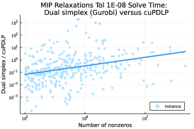
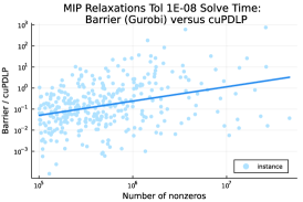
Figure 4: Ratio of Gurobi solve time over cuPDLP.jl solve time for moderate accuracy (top) and high accuracy (bottom).

Furthermore, Figure 4 visualizes the running time comparison between Gurobi and cuPDLP.jl over the size of the instances with scatter plots. Specifically, each dot in a scatter plot is an instance both methods can solve within the time limit. The x-axes are the number of nonzeros of a MIP Relaxations instance, and the y-axes are the running time ratio of Gurobi (primal simplex, dual simplex, and barrier, respectively) over cuPDLP.jl. Though with higher variance, we can observe a strong positive correlation between the speed-up of cuPDLP.jl against Gurobi versus the number of nonzeros of the problems.

4.2.2 cuPDLP.jl versus PDLP

	Small (269) (1-hour limit)		Medium (94) (1-hour limit)		Large (20) (5-hour limit)		Total (383)
	Count	Time	Count	Time	Count	Time	Count	Time
cuPDLP.jl	265	10.91	89	17.60	18	156.80	372	14.94
FirstOrderLp.jl	251	35.03	81	166.72	11	2203.72	343	67.19
PDLP (1 thread)	254	24.13	83	107.99	15	1583.54	352	46.56
PDLP (4 threads)	256	26.45	89	58.61	15	805.53	360	40.07

Table 8: Solve time in seconds and SGM10 of different solvers on instances of MIP Relaxations with tolerance $10^{-4}$: cuPDLP.jl versus PDLP.

	Small (269) (1-hour limit)		Medium (94) (1-hour limit)		Large (20) (5-hour limit)		Total (383)
	Count	Time	Count	Time	Count	Time	Count	Time
cuPDLP.jl	257	30.17	89	52.50	16	434.34	362	40.76
FirstOrderLp.jl	233	97.02	63	449.39	8	3722.08	304	174.20
PDLP (1 thread)	249	52.46	72	280.86	11	3723.40	332	102.81
PDLP (4 threads)	243	60.75	79	177.20	13	1980.16	335	96.93

Table 9: Solve time in seconds and SGM10 of different solvers on instances of MIP Relaxations with tolerance $10^{-8}$: cuPDLP.jl versus PDLP.

Tables 8 and 9 present the performance comparison of cuPDLP.jl and its CPU implementations on MIP Relaxations with tolerances of $10^{-4}$ and $10^{-8}$, respectively. The two tables demonstrate that GPU can significantly speed up PDLP, in particular for large instances:

• For moderate accuracy (Table 8), cuPDLP.jl demonstrates a 3x speed-up for small instances, a 9x speed-up for medium instances, and a 14x speed-up for large instances, compared to FirstOrderLp.jl, a CPU implementation of PDLP in Julia. When comparing cuPDLP.jl with the more delicate C++ implementation PDLP with multithreading support, it still exhibits a significant speedup for all sizes of problems. A more significant speed-up can be observed for high accuracy (Table 9).

• In terms of solved count, cuPDLP.jl solves significantly more instances regardless of the scales. In particular, comparing with FirstOrderLp.jl under tolerance $\epsilon=10^{-4}$, cuPDLP.jl solves 14 more small-sized instances, 8 more medium-sized instances and 7 more large problems, with in total 29 more instances solved. Compared to PDLP with the best of one thread or four threads, cuPDLP.jl can solve 9 more small-sized instances and 3 more large-sized instances. The improvement is more remarkable when looking at results for high accuracy $\epsilon=10^{-8}$.

In summary, the GPU-implemented cuPDLP.jl consistently outperforms the CPU-implemented PDLP in numerical performance on MIP Relaxations, with cuPDLP.jl demonstrating even more pronounced advantages on instances of medium to large scale.

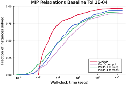
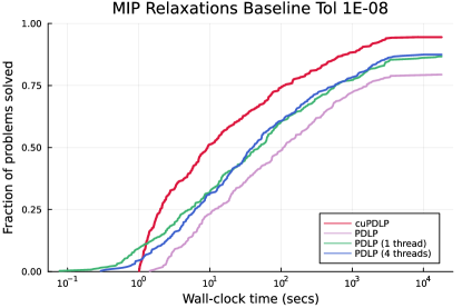
Figure 5: Number of instances solved for MIP Relaxations under moderate accuracy (left) and high accuracy (right): cuPDLP.jl versus PDLP.

Similar to Figure 3, Figure 5 demonstrates the number of solved instances of cuPDLP.jl and three CPU implementations of PDLP on MIP Relaxations in a given time. As shown in both panels, when seeking solutions with moderate accuracy ($\epsilon=10^{-4}$) and high accuracy ($\epsilon=10^{-8}$), cuPDLP.jl has a clear superior performance to all CPU versions of PDLP. Moreover, it is notable that cuPDLP.jl has a computational overhead of around one second due to the GPU kernel launch time.

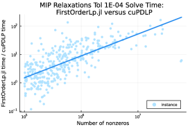
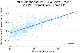
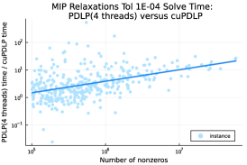
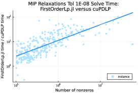
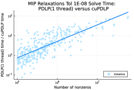
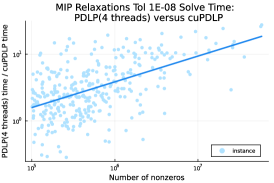
Figure 6: Ratio of PDLP solve time over cuPDLP.jl solve time for moderate accuracy (top) and high accuracy (bottom).

Furthermore, we visualize the comparison of solve time of PDLP with cuPDLP.jl in Figure 6. The y-axes are the ratio of FirstOrderLp.jl/PDLP with single thread/PDLP with four threads solve time and cuPDLP.jl solve time, which represents the speed-up gained by cuPDLP.jl, while the x-axes is the number of nonzeros in each constraint matrix. We further ran a linear regression on the data, and it turns out the slope of the fitted line equals 0.77/0.86/0.42 under moderate accuracy while equals 0.64/0.84/0.39 for high accuracy on FirstOrderLp.jl/single-threaded PDLP/four-threaded PDLP. The increasing trends in the figures imply that GPU-based cuPDLP.jl can gain more significant speed-up over CPU-based counterpart PDLP as we solve larger instances.

4.3 Mittelmann’s LP benchmark set

We further compare cuPDLP.jl with PDLP and Gurobi on Mittelmann’s LP benchmark set. Mittelmann’s LP benchmark set [44] is a standard LP benchmark to test the numerical performances of different LP solvers and includes 49 LP instances in our experiments.

Table 10 and Table 11 summarize the results on Mittelmann’s LP benchmark set. The observations are consistent with the findings on MIP Relaxations as discussed in Section 4.2. Consider the moderate accuracy. cuPDLP.jl can solve more instances against all versions of PDLP and Gurobi. When solving for high-accuracy solutions, the performance of cuPDLP.jl still performs comparable to Gurobi, only inferior to Gurobi barrier but superior to primal and dual simplex. This again demonstrates the robust performance of GPU-implemented cuPDLP.jl.

	Tol 1E-04		Tol 1E-08
	Count	Time	Count	Time
cuPDLP.jl	43	90.46	39	362.32
Primal simplex (Gurobi)	37	764.19	37	939.96
Dual simplex (Gurobi)	39	400.08	37	589.02
Barrier (Gurobi)	41	118.14	41	127.00

Table 10: Solve time in seconds and SGM10 of different solvers on instances of Mittelmann’s LP benchmark set with tolerance $10^{-4}$ and $10^{-8}$.

	Tol 1E-04		Tol 1E-08
	Count	Time	Count	Time
cuPDLP.jl	43	90.46	39	362.32
FirstOrderLp.jl	33	1044.81	24	2691.59
PDLP (1 thread)	39	636.53	31	1589.52
PDLP (4 threads)	40	362.27	34	1041.56

Table 11: Solve time in seconds and SGM10 of different solvers on instances of Mittelmann’s LP benchmark set with tolerance $10^{-4}$ and $10^{-8}$.

5 Conclusion and future directions

In this paper, we present cuPDLP.jl, a GPU implementation of restarted PDHG for solving LP in Julia. The numerical experiments demonstrate that the prototype GPU implementation cuPDLP.jl can have comparable performance with commercial solvers like Gurobi and superior performance on large instances. This sheds light on using GPU to develop high-performance optimization solvers. We end the paper by presenting a few future directions:

• C/C++ implementation. cuPDLP.jl is a prototype LP solver written in Julia. We anticipate an optimized GPU implementation of PDLP in C/C++ will perform significantly better and have superior behaviors than commercial solvers.

• Multiple GPUs. The current version of cuPDLP.jl is a single-GPU implementation. The size of a huge LP instance can go beyond the memory size of one GPU, and thus, a multiple-GPU MPI implementation is essential for cuPDLP.jl to solve larger instances.

• Mixed precision. Modern GPUs are equipped with cores specialized in efficient single-precision arithmetic. An interesting direction is effectively leveraging such computational power for optimization solvers.

References

- [1] Ayan Acharya, Siyuan Gao, Borja Ocejo, Kinjal Basu, Ankan Saha, Keerthi Selvaraj, Rahul Mazumdar, Parag Agrawal, and Aman Gupta, Promoting inactive members in edge-building marketplace, Companion Proceedings of the ACM Web Conference 2023, 2023, pp. 945–949.
- [2] Randy I Anderson, Robert Fok, and John Scott, Hotel industry efficiency: An advanced linear programming examination, American Business Review 18 (2000), no. 1, 40.
- [3] David Applegate, Mateo Díaz, Oliver Hinder, Haihao Lu, Miles Lubin, Brendan O’Donoghue, and Warren Schudy, Practical large-scale linear programming using primal-dual hybrid gradient, Advances in Neural Information Processing Systems 34 (2021), 20243–20257.
- [4] David Applegate, Mateo Díaz, Haihao Lu, and Miles Lubin, Infeasibility detection with primal-dual hybrid gradient for large-scale linear programming, arXiv preprint arXiv:2102.04592 (2021).
- [5] David Applegate, Oliver Hinder, Haihao Lu, and Miles Lubin, Faster first-order primal-dual methods for linear programming using restarts and sharpness, Mathematical Programming 201 (2023), no. 1-2, 133–184.
- [6] Kinjal Basu, Amol Ghoting, Rahul Mazumder, and Yao Pan, Eclipse: An extreme-scale linear program solver for web-applications, International Conference on Machine Learning, PMLR, 2020, pp. 704–714.
- [7] Tim Besard, Christophe Foket, and Bjorn De Sutter, Effective extensible programming: unleashing julia on gpus, IEEE Transactions on Parallel and Distributed Systems 30 (2018), no. 4, 827–841.
- [8] Jeff Bezanson, Alan Edelman, Stefan Karpinski, and Viral B Shah, Julia: A fresh approach to numerical computing, SIAM review 59 (2017), no. 1, 65–98.
- [9] Edward H Bowman, Production scheduling by the transportation method of linear programming, Operations Research 4 (1956), no. 1, 100–103.
- [10] Stephen Boyd, Stephen P Boyd, and Lieven Vandenberghe, Convex optimization, Cambridge university press, 2004.
- [11] Antonin Chambolle and Thomas Pock, A first-order primal-dual algorithm for convex problems with applications to imaging, Journal of mathematical imaging and vision 40 (2011), 120–145.
- [12] , On the ergodic convergence rates of a first-order primal–dual algorithm, Mathematical Programming 159 (2016), no. 1-2, 253–287.
- [13] Abraham Charnes and William W Cooper, The stepping stone method of explaining linear programming calculations in transportation problems, Management science 1 (1954), no. 1, 49–69.
- [14] Abraham Charnes, William W Cooper, and Merton H Miller, Application of linear programming to financial budgeting and the costing of funds, The Journal of Business 32 (1959), no. 1, 20–46.
- [15] Laurent Condat, A primal–dual splitting method for convex optimization involving lipschitzian, proximable and linear composite terms, Journal of optimization theory and applications 158 (2013), no. 2, 460–479.
- [16] Munther Dahleh and Ignacio Diaz-Bobillo, Control of uncertain systems: a linear programming approach, Prentice-Hall, Inc., 1994.
- [17] George B Dantzig, Linear programming, Operations research 50 (2002), no. 1, 42–47.
- [18] George Bernard Dantzig, Linear programming and extensions, vol. 48, Princeton university press, 1998.
- [19] Jerome Delson and Mohammad Shahidehpour, Linear programming applications to power system economics, planning and operations, IEEE Transactions on Power Systems 7 (1992), no. 3, 1155–1163.
- [20] Qi Deng, Qing Feng, Wenzhi Gao, Dongdong Ge, Bo Jiang, Yuntian Jiang, Jingsong Liu, Tianhao Liu, Chenyu Xue, Yinyu Ye, et al., New developments of admm-based interior point methods for linear programming and conic programming, arXiv preprint arXiv:2209.01793 (2022).
- [21] Ernie Esser, Xiaoqun Zhang, and Tony F Chan, A general framework for a class of first order primal-dual algorithms for convex optimization in imaging science, SIAM Journal on Imaging Sciences 3 (2010), no. 4, 1015–1046.
- [22] Olivier Fercoq, Quadratic error bound of the smoothed gap and the restarted averaged primal-dual hybrid gradient, (2021).
- [23] Dongdong Ge, Qi Huangfu, Zizhuo Wang, Jian Wu, and Yinyu Ye, Cardinal optimizer (copt) user guide, arXiv preprint arXiv:2208.14314 (2022).
- [24] Ambros Gleixner, Gregor Hendel, Gerald Gamrath, Tobias Achterberg, Michael Bastubbe, Timo Berthold, Philipp Christophel, Kati Jarck, Thorsten Koch, Jeff Linderoth, et al., Miplib 2017: data-driven compilation of the 6th mixed-integer programming library, Mathematical Programming Computation 13 (2021), no. 3, 443–490.
- [25] Greg Glockner, Parallel and distributed optimization with gurobi optimizer, https://www.gurobi.com/events/parallel-and-distributed-optimization-with-gurobi/, 2015.
- [26] , Does gurobi support gpus?, https://support.gurobi.com/hc/en-us/articles/360012237852-Does-Gurobi-support-GPUs-, 2023.
- [27] Fred Hanssmann and Sidney W Hess, A linear programming approach to production and employment scheduling, Management science (1960), no. 1, 46–51.
- [28] Peter Hazell and Pasquale Scandizzo, Competitive demand structures under risk in agricultural linear programming models, American Journal of Agricultural Economics 56 (1974), no. 2, 235–244.
- [29] Bingsheng He and Xiaoming Yuan, Convergence analysis of primal-dual algorithms for a saddle-point problem: from contraction perspective, SIAM Journal on Imaging Sciences 5 (2012), no. 1, 119–149.
- [30] Oliver Hinder, Worst-case analysis of restarted primal-dual hybrid gradient on totally unimodular linear programs, arXiv preprint arXiv:2309.03988 (2023).
- [31] Qi Huangfu and JA Julian Hall, Parallelizing the dual revised simplex method, Mathematical Programming Computation 10 (2018), no. 1, 119–142.
- [32] Narendra Karmarkar, A new polynomial-time algorithm for linear programming, Proceedings of the sixteenth annual ACM symposium on Theory of computing, 1984, pp. 302–311.
- [33] Youngdae Kim and Kibaek Kim, Accelerated computation and tracking of ac optimal power flow solutions using gpus, Workshop Proceedings of the 51st International Conference on Parallel Processing, 2022, pp. 1–8.
- [34] Youngdae Kim, François Pacaud, Kibaek Kim, and Mihai Anitescu, Leveraging gpu batching for scalable nonlinear programming through massive lagrangian decomposition, arXiv preprint arXiv:2106.14995 (2021).
- [35] Tianyi Lin, Shiqian Ma, Yinyu Ye, and Shuzhong Zhang, An admm-based interior-point method for large-scale linear programming, Optimization Methods and Software 36 (2021), no. 2-3, 389–424.
- [36] Qian Liu and Garrett Van Ryzin, On the choice-based linear programming model for network revenue management, Manufacturing & Service Operations Management 10 (2008), no. 2, 288–310.
- [37] Haihao Lu and Jinwen Yang, On the infimal sub-differential size of primal-dual hybrid gradient method, arXiv preprint arXiv:2206.12061 (2022).
- [38] , On a unified and simplified proof for the ergodic convergence rates of ppm, pdhg and admm, arXiv preprint arXiv:2305.02165 (2023).
- [39] , On the geometry and refined rate of primal-dual hybrid gradient for linear programming, arXiv preprint arXiv:2307.03664 (2023).
- [40] , A practical and optimal first-order method for large-scale convex quadratic programming, arXiv preprint arXiv:2311.07710 (2023).
- [41] Alan S Manne, Linear programming and sequential decisions, Management Science 6 (1960), no. 3, 259–267.
- [42] CPLEX User’s Manual, Ibm ilog cplex optimization studio, Version 12 (1987), no. 1987-2018, 1.
- [43] Vahab Mirrokni, Google research, 2022 & beyond: Algorithmic advances, https://ai.googleblog.com/2023/02/google-research-2022-beyond-algorithmic.html, 2023-02-10.
- [44] Hans D Mittelmann, Decision tree for optimization software., https://plato.asu.edu/bench.html, 2023.
- [45] NVIDIA, Cuda c++ best practices guide, (2023).
- [46] Brendan O’Donoghue, Operator splitting for a homogeneous embedding of the linear complementarity problem, SIAM Journal on Optimization 31 (2021), no. 3, 1999–2023.
- [47] Brendan O’Donoghue, Eric Chu, Neal Parikh, and Stephen Boyd, Conic optimization via operator splitting and homogeneous self-dual embedding, Journal of Optimization Theory and Applications 169 (2016), no. 3, 1042–1068.
- [48] Gurobi Optimization et al., Gurobi optimizer reference manual, 2023.
- [49] François Pacaud, Sungho Shin, Michel Schanen, Daniel Adrian Maldonado, and Mihai Anitescu, Accelerating condensed interior-point methods on simd/gpu architectures, Journal of Optimization Theory and Applications (2023), 1–20.
- [50] Thomas Pock and Antonin Chambolle, Diagonal preconditioning for first order primal-dual algorithms in convex optimization, 2011 International Conference on Computer Vision, IEEE, 2011, pp. 1762–1769.
- [51] Rohan Ramanath, S Sathiya Keerthi, Yao Pan, Konstantin Salomatin, and Kinjal Basu, Efficient vertex-oriented polytopic projection for web-scale applications, Proceedings of the AAAI Conference on Artificial Intelligence, vol. 36, 2022, pp. 3821–3829.
- [52] Daniel Ruiz, A scaling algorithm to equilibrate both rows and columns norms in matrices, Tech. report, CM-P00040415, 2001.
- [53] Sungho Shin, François Pacaud, and Mihai Anitescu, Accelerating optimal power flow with gpus: Simd abstraction of nonlinear programs and condensed-space interior-point methods, arXiv preprint arXiv:2307.16830 (2023).
- [54] Kasia Świrydowicz, Eric Darve, Wesley Jones, Jonathan Maack, Shaked Regev, Michael A Saunders, Stephen J Thomas, and Slaven Peleš, Linear solvers for power grid optimization problems: a review of gpu-accelerated linear solvers, Parallel Computing 111 (2022), 102870.
- [55] Peng Zhou and Beng Wah Ang, Linear programming models for measuring economy-wide energy efficiency performance, Energy Policy 36 (2008), no. 8, 2911–2916.
- [56] Mingqiang Zhu and Tony Chan, An efficient primal-dual hybrid gradient algorithm for total variation image restoration, UCLA Cam Report 34 (2008), 8–34.