FDDM: Unsupervised Medical Image Translation with a Frequency-Decoupled Diffusion Model

Abstract

Diffusion models have demonstrated significant potential in producing high-quality images for medical image translation to aid disease diagnosis, localization, and treatment. Nevertheless, current diffusion models have limited success in achieving faithful image translations that can accurately preserve the anatomical structures of medical images, especially for unpaired datasets. The preservation of structural and anatomical details is essential to reliable medical diagnosis and treatment planning, as structural mismatches can lead to disease misidentification and treatment errors. In this study, we introduced a frequency-decoupled diffusion model (FDDM), a novel framework that decouples the frequency components of medical images in the Fourier domain during the translation process, to allow structure-preserved high-quality image conversion. FDDM applies an unsupervised frequency conversion module to translate the source medical images into frequency-specific outputs and then uses the frequency-specific information to guide a following diffusion model for final source-to-target image translation. We conducted extensive evaluations of FDDM using a public brain MR-to-CT translation dataset, showing its superior performance against other GAN-, VAE-, and diffusion-based models. Metrics including the Fréchet inception distance (FID), the peak signal-to-noise ratio (PSNR), and the structural similarity index measure (SSIM) were assessed. FDDM achieves an FID of 29.88, less than half of the second best. These results demonstrated FDDM’s prowess in generating highly-realistic target-domain images while maintaining the faithfulness of translated anatomical structures.

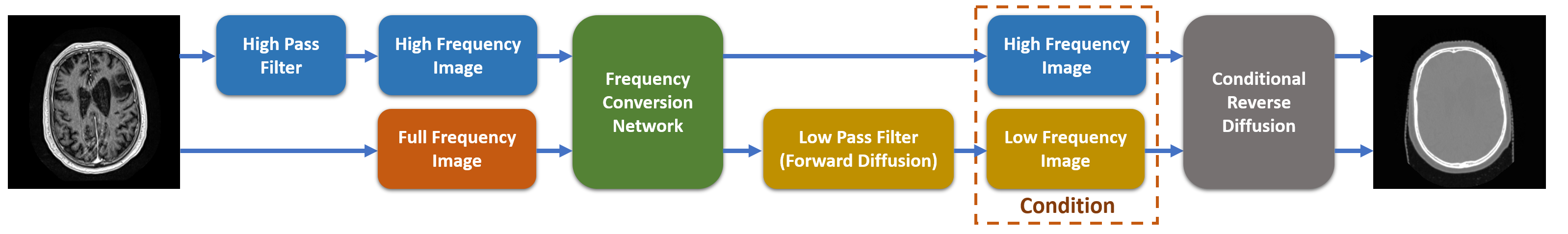
Figure 1: Overview of the FDDM framework for the MR-to-CT translation. We first converted the MR image into a high-frequency CT image and a full-frequency CT image as two separate output channels, using an unsupervised frequency conversion module. Subsequently, the full-frequency CT image was fed into a forward diffusion process (serving as a low-pass filter) to extract the low-frequency information. The low-frequency information was used as the starting step to initiate a reverse diffusion process, which was conditioned by the high-frequency CT information, to generate a final CT image.

1 Introduction

Magnetic Resonance (MR) and Computed Tomography (CT) imaging are playing pivotal and complementary roles in medical diagnosis and treatment planning [12, 19, 26, 6, 20, 22, 29, 21]. MR offers exceptional soft-tissue contrast while CT is usually preferred for bony anatomy scans. For radiation therapy, MR scans are often used for tumor localization and segmentation, while CT scans provide electron density information for calculating radiotherapy plan doses [2, 4, 27]. Current clinical practices usually acquire MR and CT as separate scans to serve different needs, incurring additional imaging time, imaging radiation dose (from CT), and medical costs. These sequential acquisitions also introduce MR/CT misregistrations that affect the alignment and localization of anatomies. The prospect of acquiring a single modality (for instance, MR), and converting it to another modality (CT) via numerical methods (MR-to-CT translation) can fundamentally address the above-mentioned challenges. However, such MR-to-CT translation remains challenging due to substantial differences between MR and CT scans in terms of image intensities and features.

The current mainstream image translation methods are generally based on generative adversarial networks (GAN) [7] or variational autoencoders (VAE) [13]. These methods show advantages in preserving the anatomical structures (high faithfulness). However, they are subject to many issues including pattern collapse, premature discriminator convergence, or resolution degradation, affecting the quality of the translated images (low realism). Recently, diffusion models demonstrated superior generative capabilities, achieving impressive Frechet Inception Distance scores (FID) that measure the realism of generated images [8, 3, 28, 25, 24]. A representative diffusion framework is the Denoising Diffusion Probabilistic Model (DDPM) [9], which utilizes a Markov chain Monte Carlo (MCMC) process to progressively add Gaussian noises to images (forward diffusion), followed by a learned reverse diffusion process that maps noises back to images. However, despite their potential, diffusion models have found significant challenges in medical image applications, particularly in preserving and maintaining the integrity of anatomical structures during image translations (low faithfulness). The forward diffusion process, where random Gaussian noises are continuously added, gradually obliterates structural details of high spatial frequencies. Such structural information is crucial for medical diagnosis/treatment, and is difficult for the reverse diffusion process to completely restore. In general, diffusion models, while excelling in creating highly realistic images, often struggle to maintain the faithfulness of translated anatomical structures. It is especially difficult to develop diffusion models on unpaired imaging datasets, which lack image pairs of well-corresponded anatomy to serve as additional clues for network training. However, unpaired datasets are far more prevalent and easier to obtain in medicine than paired datasets. Thus, a diffusion model that can learn accurate image-to-image translations from unpaired datasets (unsupervised learning) is highly desired. To address this unmet need, we proposed a novel diffusion model-based approach to achieve unsupervised image-to-image translation. The approach, named frequency-decoupled diffusion model (FDDM), uses decoupled spatial frequency information of medical images to guide anatomy-preserving image translation. We built FDDM on MR-to-CT conversions, although the same framework is readily applicable to other image translation scenarios. FDDM is composed of an unsupervised frequency conversion module and a DDPM-based diffusion model. The unsupervised frequency conversion module, which can be GAN- or VAE-based, performs an initial MR-to-CT conversion. Based on the pros/cons of the GAN- or VAE-based methods, such conversion can generate CT images of high anatomical accuracy (faithfulness), but suffers from low image quality (realism). By FDDM, the frequency conversion module outputs two channels, one with high-frequency CT information (as in the Fourier domain), and the other with full-frequency CT information. The high-frequency CT information, which correlates with the anatomical structure boundaries, leverages the advantage of the GAN- or VAE-based frequency conversion module in preserving anatomies, which can be used to condition the following diffusion model to retain the anatomy. The full-frequency CT, on the other hand, is fed into a forward diffusion process corresponding to the following diffusion model. The forward diffusion serves as a low-pass filter that captures the overall CT intensities and semantic contents. Its output is then used by the diffusion model as a starting step for the reverse diffusion, to gradually recover the middle-frequency information of the CT image, conditioned by the high-frequency CT information. Compared with the original full-frequency CT generated by the unsupervised frequency conversion module, the new CT generated by the conditioned diffusion model has boosted realism and image quality, while retaining accurate anatomical structures. In summary, our key contributions are:
1. We introduced a novel frequency-decoupled diffusion model (FDDM) for unsupervised MR-to-CT image translation. FDDM generates highly realistic images in the target CT domain, while preserving the integrity of anatomical structures from the source MR domain. By leveraging the structure preservation capability of the frequency conversion module and the realistic image generation advantage of the diffusion model, FDDM achieves both high realism and high faithfulness in the translated images.
2. With theoretical proof that the forward diffusion process of diffusion models can be approximated as a low-pass filter, the high-frequency information extracted from the frequency conversion module allows additional anatomical structure preservation. In addition, through a flexible scheme, the low- and high-frequency CT information outputs from the frequency conversion module can be selectively introduced into the diffusion model to allow the model to further correct their residual errors in the final translated CT image.
3. FDDM demonstrated superior performance in MR-to-CT translation compared to existing state-of-the-art methods, including those based on GANs, VAEs, and other diffusion models.

2 Related Work

2.1 Unsupervised Medical Image Translation.

Image-to-image translation has been widely employed in medical applications, including but not limited to tumor and organ segmentation, cross-modal image registration, low-dose CT denoising, fast MR reconstruction, and metal artifact reduction [1, 11]. For medical image translation, it is critical to preserve the integrity of anatomical structures when converting images between domains. The primary methods including Generative Adversarial Networks (GANs)  [7] and Variational Autoencoders (VAEs) generally perform well in structure retention (high faithfulness) [13]. Notable developments in GAN-based methods include CycleGAN [31] which promotes cyclic consistency; and GCGAN [5] for unilateral, geometry-consistent mapping. Additionally, RegGAN [14] blends image translation with registration. Despite much success, GANs often face training instability that reduces the quality of generated images (low realism). In addition to GANs, VAE-based approaches like UNIT [16] and MUNIT [10] share similar advantages/disadvantages.

2.2 Diffusion Models for Image Translation

Recently, diffusion models have emerged as powerful tools in generating high-quality and realistic images, surpassing GANs and VAEs. One example of the diffusion model is SDEdit [17] , which translates images through iterative denoising via stochastic differential equations. Another diffusion model, EGSDE [30], guides unpaired image translation with pre-trained energy features, balancing realism and faithfulness of translated images. In medical image translation, SynDiff [18] represents a significant advancement with its adversarial diffusion design, although its dependence on a separate CycleGAN model for paired data synthesis has limited its performance. Li et al. [15] proposed a novel framework for zero-shot medical image translation based on the diffusion model, which only requires target domain images for training. However, it is built on the assumption that the source domain and the target domain share most of the low- and high-frequency information, which is not true in the MR-to-CT translation task. In general, GANs and VAEs tend to better preserve the anatomy (faithfulness), while diffusion models generate images of superior realism. Improving the capability of diffusion models in preserving the anatomy can maximize the realism and faithfulness of the translated images. FDDM is developed to combine the benefit of VAEs or GANs in structure preservation, and the advantage of diffusion models in boosting the realism of the translated images.

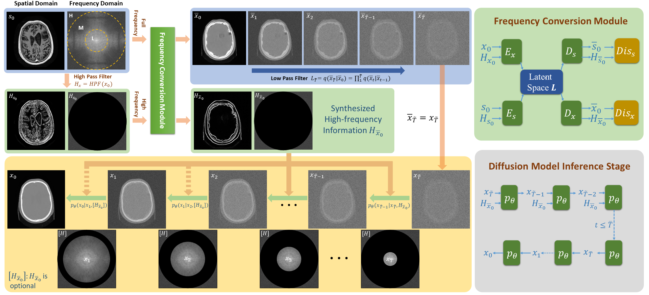
Figure 2: This figure shows the detailed framework of our FDDM, in which $\tilde{T}$ and $\overline{T}$ can be freely selected during the inference stage, allowing us to select the suitable $\tilde{T}$ and $\overline{T}$ based on the error ratio of the generated low-frequency and high-frequency information.

3 Method

Given a source MR image $s_{0}$ and a target CT image $x_{0}$, we used an unsupervised frequency conversion module that transformed the high-frequency and full-frequency information of the MR image into the counterparts of the CT image. The frequency conversion module can be either GAN- or VAE-based, which excels in structure preservation. In our implementation of FDDM, we used UNIT, a VAE-based framework. Following this, the transformed full-frequency CT image was input into the forward diffusion process, which functions as a low-pass filter for low-frequency information extraction. This low-frequency information is used by the diffusion model as the starting step for reversed diffusion. The reverse diffusion, conditioned by the high-frequency CT information from the frequency conversion module, generates the final translated CT image. In the following paragraphs, we first described the diffusion model basics and the frequency filters, with theoretical proof that the forward diffusion process of diffusion models functions as a low-pass filter. Then we described the MR-to-CT frequency conversion module used by FDDM, based on the VAE with cycle consistency. Following the frequency conversion module, we introduced the unique, flexible frequency conditioning scheme employed in FDDM to maximize the accuracy of translated images and correct the residual errors from the frequency conversion module.

3.1 Diffusion Models and Filters for Frequency Decoupling

Diffusion models, as discussed in several studies [23, 9, 24], use a forward diffusion procedure $q(\cdot)$, which progressively introduces white Gaussian noise with a constant variance $I$ to the initial image $x_{0}$ through $T$ steps:

$$q(x_{1:T}|x_{0})=\prod_{t=1}^{T}q(x_{t}|x_{t-1})$$ (1)

$$q(x_{t}|x_{t-1})=\mathcal{N}\left(x_{t};\sqrt{\frac{\alpha_{t}}{\alpha_{t-1}}}x_{t-1},(1-\frac{\alpha_{t}}{\alpha_{t-1}})I\right)$$ (2)

$x_{t}$ denotes the noise-corrupted image at step $t$. The sequence $\alpha_{1:t}$ decreases monotonically and stays within $(0,1]^{T}$. The reverse denoising (diffusion) process, $p_{\theta}(\cdot)$, is then detailed as:

$$p_{\theta}(x_{0:T})=p(x_{T})\prod_{t=1}^{T}p_{\theta}(x_{t-1}|x_{t})$$ (3)

The terms $\boldsymbol{\mu}_{\theta}(x_{t},t)$ and ${\Sigma}_{\theta}(x_{t},t)$ denote the mean and variance of the denoising model, respectively, with $\theta$ denoting its parameters.

By referencing the study of Ho et al. [9], the forward diffusion process can be viewed as a Markov chain with Gaussian transitions, regulated by the descending sequence $\alpha_{1:t}$. Derived from Eq. 2, a specific attribute of the forward process can be expressed as:

$$q(x_{t}|x_{0})=\mathcal{N}(x_{t};\sqrt{\alpha_{t}}x_{0},(1-\alpha_{t})I)$$ (4)

Following this, we can represent $x_{t}$ as:

$$x_{t}=\sqrt{\alpha_{t}}x_{0}+\sqrt{1-\alpha_{t}}z,\quad\quad z\sim\mathcal{N}(0,I)$$ (5)

with $z$ represents the white Gaussian noise. In the frequency spectrum:

$$\mathcal{F}[x_{t}] =\sqrt{\alpha_{t}}\mathcal{F}[x_{0}]+\sqrt{1-\alpha_{t}}\mathcal{F}[z]$$ (6)

$$\mathcal{X}_{t}(u,v) =\sqrt{\alpha_{t}}\mathcal{X}_{0}(u,v)+\sqrt{1-\alpha_{t}}\mathcal{Z}(u,v)$$ (7)

$\mathcal{F}$ denotes Fourier transforms, and $\mathcal{X}_{t}(u,v)$, $\mathcal{X}_{0}(u,v)$, and $\mathcal{Z}(u,v)$ are the corresponding frequency domain representations. For white Gaussian noise $\mathcal{Z}(u,v)$, the expectation and variance are:

$$E[Z(u,v)] =0$$ (8)

$$Var[Z(u,v)] =I$$ (9)

The autocorrelation function of the white Gaussian noise can be articulated as:

$$R_{N}(\tau_{1},\tau_{2}) =\int\mathcal{Z}(u,v)\mathcal{Z}(u-\tau_{1},v-\tau_{2})dudv$$ (10)

$$=\int I\delta(\tau_{1},\tau_{2})dudv$$ (11)

$$=I\delta(\tau_{1},\tau_{2})$$ (12)

Given that $\delta(\tau_{1},\tau_{2})$ represents the Dirac delta function, the white Gaussian noise has uniform power across all frequency bands. In general images, the power spectral density (PSD) is inversely proportional to the spatial frequency:

$$PSD(u,v)_{x_{0}}=\frac{k}{\|(u,v)\|^{a}}$$ (13)

where $k$ and $a$ are scaling/modifying factors. When noise is introduced to the image, the PSD of the noise gets combined with the PSD of the image. Thus, defining signal-to-noise ratio (SNR) at step $t$:

$$SNR_{t}=\frac{\sqrt{\alpha_{t}}k}{\sqrt{1-\alpha_{t}}\|(u,v)\|^{a}I}$$ (14)

Since $\alpha_{t}$ is monotonically decreasing with diffusion steps, when the diffusion step $t$ increases, the SNR decreases. Given a threshold SNR $\phi$, beyond a specific step $t$, only low-frequency information remains:

$$SNR_{t}\left\{\begin{aligned} <&\phi&\|(u,v)\|>&\psi\\ \geq&\phi&\|(u,v)\|&\leq\psi\\ \end{aligned}\right.$$ (15)

If we denote this step as $\tilde{T}$, then the forward diffusion mirrors the effect of a low-pass filter:

$$x_{\tilde{T}}=LPF_{\tilde{T}}(x_{0})=q(x_{\tilde{T}}|x_{0})$$ (16)

Approximately, we can regard the reverse diffusion as a reverse low-pass filter:

$$x_{0}=RLPF_{\tilde{T}}(x_{\tilde{T}})=p_{\theta}(x_{0}|x_{\tilde{T}})$$ (17)

For FDDM, a high-pass filter, the Sobel operator, is employed to extract high-frequency information. This operator acts as a discrete differential operator, effectively calculating the image’s intensity gradient to extract high-frequency components.

$$H_{x_{0}}=HPF(x_{0})=Sobel(x_{0})$$ (18)

Based on the output from the forward diffusion process, which functions as a low-pass filter, the low-frequency CT information can be extracted as the starting step of the diffusion model for the reversed diffusion. Concurrently, the high-frequency CT information can be extracted by the Sobel filter to condition the reverse diffusion process to retain the anatomical structures. In this regard, the diffusion model can be solely trained on the CT domain, without using any information from the MR domain. However, since the low- and high-frequency information of MRs does not match that of CTs, we need to further convert such information of MRs to CTs via another frequency conversion module prior to the CT-only diffusion model, which was described below.

3.2 Frequency Conversion Module

Since the MR and CT have vastly different information at the full frequency spectrum, we can not use a diffusion model trained solely on the CT information to convert MR to CT. However, we can first convert the MR to CT via a frequency conversion module, and then extract low- and high-frequency information from the converted CT image to feed into a CT-trained diffusion model to generate a fine-tuned CT output. We built our frequency conversion module based on a widely-used VAE framework with cycle consistency [16]. Specifically, our frequency conversion module has two encoders $E_{s}$, $E_{x}$, two decoders $D_{s}$, $D_{x}$, and two discriminators $Dis_{s},Dis_{x}$, based on the hypothesis of a shared-latent space $L$ between two encoders and two decoders, as depicted in Figure 2. This latent space can be independently derived from each domain and from this latent space, the full-frequency images and high-frequency images of both MR and CT can be regenerated. Specifically, we posit the existence of the following functions:

$$L_{s}=E_{s}(s_{0},H_{s_{0}})=L_{x}=E_{x}(x_{0},H_{x_{0}})$$ (19)

$$\overline{s}_{0},H_{\overline{s}_{0}}=D_{s}(L_{x})=D_{s}(E_{x}(x_{0},H_{x_{0}}))$$ (20)

$$\overline{x}_{0},H_{\overline{x}_{0}}=D_{x}(L_{s})=D_{x}(E_{s}(s_{0},H_{s_{0}}))$$ (21)

The training details of our frequency conversion module are in Supplementary Materials A.

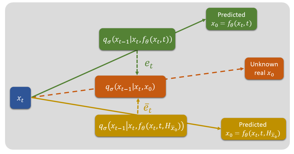
Figure 3: Schematic diagram of minimizing reverse diffusion errors.

3.3 Minimizing Reverse Diffusion Errors by Flexible Frequency Conditioning

After we obtain the full-frequency image $\overline{x}_{0}$ and the high-frequency image $H_{\overline{x}_{0}}$ of CT through the frequency conversion module, the low-frequency CT image $\overline{x}_{\tilde{T}}$ is further derived through the forward diffusion (low-pass filtering) of $\overline{x}_{0}$. Compared with conventional diffusion model setups, FDDM designs a frequency information conditioning scheme to introduce and remove the conditioning information $H_{\overline{x}_{0}}$ flexibly during the reverse diffusion process, which can help to correct residual errors of $H_{\overline{x}_{0}}$.

To predict $x_{0}$ from a noisy $x_{t}$ via the reverse diffusion, $x_{t-1}$ is generated via the reverse conditional distribution $q_{\sigma}(x_{t-1}|x_{t},x_{0})$, with an intermediately predicted $x_{0}$. $\sigma$ denotes a parameter that adjusts the update scheme. Based on [24], we can define $q_{\sigma}(x_{t-1}|x_{t},x_{0})$ as:

$$\begin{split}q_{\sigma}(x_{t-1}|x_{t},x_{0})=&\mathcal{N}\left(\sqrt{\alpha_{t-1}}x_{0}+\right.\\ &\left.\sqrt{1-\alpha_{t-1}-\sigma^{2}_{t}}\cdot\frac{x_{t}-\sqrt{\alpha_{t}}x_{0}}{\sqrt{1-\alpha_{t}}},\sigma_{t}^{2}I\right)\end{split}$$ (22)

The reverse diffusion process $p_{\theta}^{(t)}(x_{t-1}|x_{t})$ is a trainable generative process, which leverages the knowledge of $q_{\sigma}(x_{t-1}|x_{t},x_{0})$.

$$p_{\theta}^{(t)}(x_{t-1}|x_{t})=q_{\sigma}(x_{t-1}|x_{t},f_{\theta}(x_{t},t))\quad(t>1)$$ (23)

Based on Eq 5, we can predict $x_{0}$ given $x_{t}$ through the following equation:

$$x_{0}=f_{\theta}(x_{t},t):=(x_{t}-\sqrt{1-\alpha_{t}}\cdot\epsilon_{\theta}(x_{t},t))/\sqrt{\alpha_{t}}$$ (24)

where $\epsilon_{\theta}$ is our model, and during its training, the high-frequency information $H_{\overline{x}_{0}}$ can be introduced as a condition:

$$x_{0}=f_{\theta}(x_{t},t,H_{\overline{x}_{0}}):=(x_{t}-\sqrt{1-\alpha_{t}}\cdot\epsilon_{\theta}(x_{t},t,H_{\overline{x}_{0}}))/\sqrt{\alpha_{t}}$$ (25)

$$p_{\theta}^{(t)}(x_{t-1}|x_{t},H_{\overline{x}_{0}})=q_{\sigma}(x_{t-1}|x_{t},f_{\theta}(x_{t},t,H_{\overline{x}_{0}}))\quad(t>1)$$ (26)

We optimized $\theta$ via the following variational inference objective:

$$\begin{split}&J_{\sigma}(\epsilon_{\theta}):=\\ &\ \mathbb{E}_{x_{0:T}\sim q_{\sigma}(x_{0:T})}\left[\log q_{\sigma}(x_{T}|x_{0})+\sum_{t=2}^{T}\log q_{\sigma}(x_{t-1}|x_{t},x_{0})\right.\\ &\left.-\sum_{t=1}^{T}\log p_{\theta}^{(t)}(x_{t-1}|x_{t},[H_{\overline{x}_{0}}])-\log p_{\theta}(x_{T})\right]\end{split}$$ (27)

where $[H_{\overline{x}_{0}}]$ indicates that $H_{\overline{x}_{0}}$ is optional for the model during the training process. Specifically, we randomly put $H_{\overline{x}_{0}}$ or $-1$ values (no condition). Our reverse conditional distribution includes adding high-frequency information or not, shown as:

$$\begin{split}&q_{\sigma}(x_{t-1}|x_{t},f_{\theta}^{(t)}(x_{t}))=\mathcal{N}\Bigg{(}\sqrt{\alpha_{t-1}}f_{\theta}^{(t)}(x_{t})+\\ &\sqrt{1-\alpha_{t-1}-\sigma^{2}_{t}}\cdot\frac{x_{t}-\sqrt{\alpha_{t}}f_{\theta}^{(t)}(x_{t})}{\sqrt{1-\alpha_{t}}},\sigma_{t}^{2}I\Bigg{)}\end{split}$$ (28)

$$\begin{split}&q_{\sigma}(x_{t-1}|x_{t},f_{\theta}^{(t)}(x_{t},H_{\overline{x}_{0}}))=\mathcal{N}\Bigg{(}\sqrt{\alpha_{t-1}}f_{\theta}^{(t)}(x_{t},H_{\overline{x}_{0}})+\\ &\sqrt{1-\alpha_{t-1}-\sigma^{2}_{t}}\cdot\frac{x_{t}-\sqrt{\alpha_{t}}f_{\theta}^{(t)}(x_{t},H_{\overline{x}_{0}})}{\sqrt{1-\alpha_{t}}},\sigma_{t}^{2}I\Bigg{)}\end{split}$$ (29)

Inputs: The source image $s_{0}$, VAE Encoders $E_{s}$, VAE Decoders $D_{x}$, Pre-trained denoising diffusion model $p_{\theta}$, High pass filter $HPF(\cdot)$, Low pass filter $LPF(\cdot)$, High-frequency information $H_{s_{0}}$;

Output: Converted image $x_{0}$ in the target domain;

Initialize all parameters and variables;

1:  $H_{s_{0}}\leftarrow HPF(s_{0})$

2:  $\overline{x}_{0},H_{\overline{x}_{0}}\leftarrow D_{x}(E_{s}(s_{0},H_{s_{0}}))$

3:  $x_{\tilde{T}}\leftarrow LPF_{\tilde{T}}(\overline{x}_{0})$

4:  for $t=\tilde{T}$ down to $\overline{T}$ do

5:     $x_{t-1}\leftarrow p_{\theta}^{(t)}(x_{t-1}|x_{t},H_{\overline{x}_{0}})$

6:  end for

7:  for $t=\overline{T}$ down to $1$ do

8:     $x_{t-1}\leftarrow p_{\theta}^{(t)}(x_{t-1}|x_{t})$

9:  end for

10:  return  $x_{0}$

Algorithm 1 Inference Process for FDDM

We define $e_{t}$ and $\overline{e}_{t}$ as the error terms for the reverse diffusion process at each time step $t$. These terms measure the discrepancy between the actual reverse process and our model’s prediction, with $\overline{e}_{t}$ considering the additional high-frequency information $H_{\overline{x}_{0}}$.

$$\begin{split}&e_{t}=||q_{\sigma}(x_{t-1}|x_{t},x_{0})-q_{\sigma}(x_{t-1}|x_{t},f_{\theta}(x_{t},t))||\\ &=\Bigg{\|}\mathcal{N}\Bigg{(}\sqrt{\alpha_{t-1}}x_{0}+\sqrt{1-\alpha_{t-1}-\sigma^{2}_{t}}\cdot\frac{x_{t}-\sqrt{\alpha_{t}}x_{0}}{\sqrt{1-\alpha_{t}}},\sigma_{t}^{2}I\Bigg{)}-\\ &\mathcal{N}\Bigg{(}\sqrt{\alpha_{t-1}}\frac{x_{t}-\sqrt{1-\alpha_{t}}\cdot\epsilon_{\theta}(x_{t},t)}{\sqrt{\alpha_{t}}}+\\ &\sqrt{1-\alpha_{t-1}-\sigma^{2}_{t}}\cdot\frac{x_{t}-\sqrt{\alpha_{t}}\left(\frac{x_{t}-\sqrt{1-\alpha_{t}}\cdot\epsilon_{\theta}(x_{t},t)}{\sqrt{\alpha_{t}}}\right)}{\sqrt{1-\alpha_{t}}},\sigma_{t}^{2}I\Bigg{)}\Bigg{\|}\end{split}$$ (30)

$$\begin{split}&\overline{e}_{t}=||q_{\sigma}(x_{t-1}|x_{t},x_{0})-q_{\sigma}(x_{t-1}|x_{t},f_{\theta}(x_{t},t,H_{\overline{x}_{0}}))||\\ &=\Bigg{\|}\mathcal{N}\Bigg{(}\sqrt{\alpha_{t-1}}x_{0}+\sqrt{1-\alpha_{t-1}-\sigma^{2}_{t}}\cdot\frac{x_{t}-\sqrt{\alpha_{t}}x_{0}}{\sqrt{1-\alpha_{t}}},\sigma_{t}^{2}I\Bigg{)}-\\ &\mathcal{N}\Bigg{(}\sqrt{\alpha_{t-1}}\frac{x_{t}-\sqrt{1-\alpha_{t}}\cdot\epsilon_{\theta}(x_{t},t,H_{\overline{x}_{0}})}{\sqrt{\alpha_{t}}}+\\ &\sqrt{1-\alpha_{t-1}-\sigma^{2}_{t}}\cdot\frac{x_{t}-\sqrt{\alpha_{t}}\left(\frac{x_{t}-\sqrt{1-\alpha_{t}}\cdot\epsilon_{\theta}(x_{t},t,H_{\overline{x}_{0}})}{\sqrt{\alpha_{t}}}\right)}{\sqrt{1-\alpha_{t}}},\sigma_{t}^{2}I\Bigg{)}\Bigg{\|}\end{split}$$ (31)

The minimum error term $e_{min}$ is then determined at each step. Since we use high-frequency information as a condition, our reverse diffusion can be approximately viewed as a reverse low-pass filter. We assume that there is $\overline{T}$, and when $T<\overline{T}$, the relationship between $\overline{e}$ and $e$ changes, shown as Figure 3.

$$\begin{split}e_{min}=Min(e_{t},\overline{e}_{t})=\begin{cases}\overline{e}_{t}&\text{if }t\geq\overline{T},\\ e_{t}&\text{if }x<\overline{T}.\end{cases}\end{split}$$ (32)

Throughout the reverse diffusion steps, the total errors without/with $H_{\overline{x}_{0}}$ are defined as $E$ and $\overline{E}$.

$$\begin{split}E=\sum_{t=0}^{T}e_{t},\quad\overline{E}=\sum_{t=0}^{T}\overline{e}_{t}\end{split}$$ (33)

$E_{min}$ refers to the minimizing of the error in the entire reverse diffusion, as shown below:

$$\begin{split}E_{min}=\sum_{t=0}^{T}e_{min}=\sum_{t=0}^{\overline{T}}e_{t}+\sum_{t=\overline{T}}^{T}\overline{e}_{t}\end{split}$$ (34)

The derivation shows that there exists an optimal step $\overline{T}$ during the reverse diffusion, beyond which dropping the high-frequency condition can further reduce the errors in the translated image, which can be customized during test-time optimization. In summary, the whole MR-to-CT translation process is shown in Algorithm 1.

4 Experiments

Details of the dataset and implementation are given in Supplementary Materials B and C.

Method	FID $\downarrow$	SSIM $\uparrow$	PSNR $\uparrow$
GCGAN	100.1453	0.8012 $\pm$ 0.0584	35.5610 $\pm$ 1.5398
RegGAN	71.8493	0.7748 $\pm$ 0.0987	35.0037 $\pm$ 1.2602
CycleGAN	65.4173	0.7779 $\pm$ 0.0544	35.1246 $\pm$ 1.0129
UNIT	67.9931	0.7905 $\pm$ 0.0579	35.3229 $\pm$ 1.5297
MUNIT	82.5412	0.7516 $\pm$ 0.0678	34.9922 $\pm$ 1.2491
SynDiff	93.2486	0.8082 $\pm$ 0.0580	36.0907 $\pm$ 2.1146
SDEdit	96.7234	0.7302 $\pm$ 0.0739	34.8021 $\pm$ 2.2519
EGSDE	150.5618	0.6965 $\pm$ 0.0675	33.7938 $\pm$ 2.2106
FDDM	29.8828	0.8255 $\pm$ 0.0544	36.4282 $\pm$ 1.7404

Table 1: Comparison of different methods on the brain MR-to-CT translation dataset.

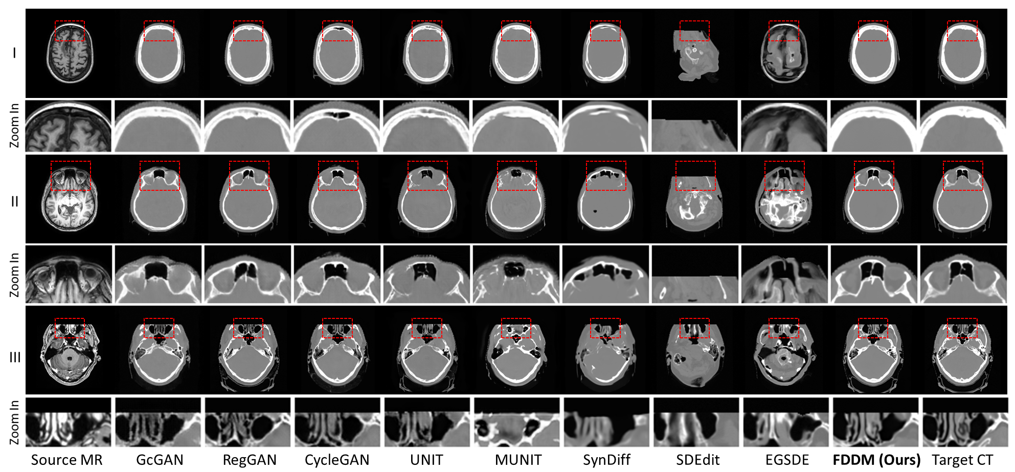
Figure 4: Visual comparison between other models and FDDM on the brain MR-to-CT translation task.

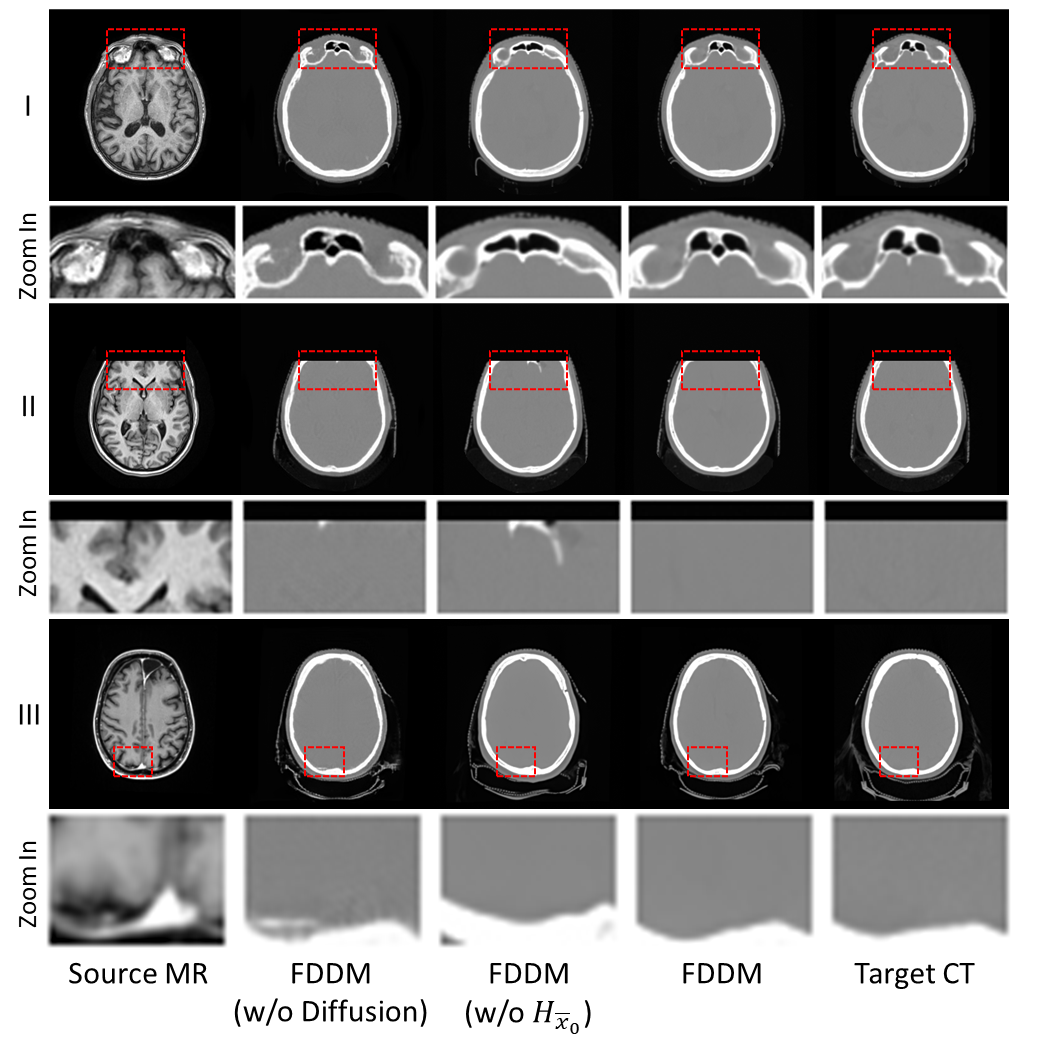
Figure 5: Visual comparison results of the ablation experiments.

Method	FID $\downarrow$	SSIM $\uparrow$	PSNR $\uparrow$
FDDM (w/o $H_{\overline{x}_{0}}$)	27.9878	0.8044 $\pm$ 0.0585	36.0336 $\pm$ 1.7653
FDDM (w/o Diffusion)	56.8436	0.7873 $\pm$ 0.0525	35.9617 $\pm$ 1.7167
FDDM	29.8828	0.8255 $\pm$ 0.0544	36.4282 $\pm$ 1.7404

Table 2: Ablation study of FDDM.

4.1 Comparison with other methods

Table 1 quantitatively compares FDDM with eight other image translation methods on FID, SSIM, and PSNR. Among them, GcGAN, CycleGAN, and RegGAN are GAN-based methods; UNIT and MUNIT are VAE-based methods; and SynDiff, SDEdit, and EGSDE are diffusion-based methods. Compared with FDDM, the GAN- and VAE-based methods presented worse FID scores (higher values), showing the challenges of these methods in generating highly realistic domain images. In contrast, these methods presented similar results to FDDM in SSIM, a structure similarity metric, matching the expectations that GANs and VAEs are good at preserving the anatomy (faithfulness), though still surpassed by FDDM. Among the three diffusion models used for comparison, SynDiff generated the best results in SSIM, as it used CycleGAN to synthesize paired MR-CT data to circumvent the challenges of unsupervised training, thus gaining a relative advantage in structure preservation. However, the introduction of CycleGAN for paired CT synthesis introduces an upper limit on imaging realism, negatively impacting SynDiff’s FID scores. Both SDEdit and EGSDE presented poor SSIM results, showing the challenge of structure retention for unsupervised training, which in turn affects realistic image generation and leads to poor FID scores. Among all methods, FDDM showed superior performance with the lowest FID score of 29.88, coupled with the highest SSIM and PSNR scores. The exceptional performance of FDDM underscores its ability to adeptly maintain the realism and faithfulness of generated images, by combining the structure preservation advantage of the frequency conversion module and the imaging realism advantage of the diffusion model (Figure 4). Compared with the SynDiff approach, which relies on the full-frequency information of a CycleGAN-generated CT to train the diffusion model, FDDM only uses selected frequency information from a GAN- or VAE-based MR-to-CT conversion network and fills in the other information via a diffusion model trained on true CT images to boost the image realism. On the other hand, the best overall SSIM scores of FDDM offered strong support to the theoretical derivations of Sec. 3.3, proving that the flexible frequency-conditioning design of FDDM not only helps to fill in the missing-frequency information but improves further on the frequency information passed from the frequency conversion module.

4.2 Ablation Study of the diffusion model and the high-frequency conditioning

FDDM integrates a unique approach that uses high- and low-frequency information outputs from the MR-CT frequency conversion module to generate a final CT image of all frequencies. The high- and low-frequency information serves as crucial conditioning inputs within the diffusion process. To access the impacts of these inputs, we performed an ablation study. Results of these ablation experiments were summerized in Table 2 and Figure 5. We first directly tested the performance of generated full-frequency images from the frequency conversion module (without diffusion), shown as FDDM w/o Diffusion in Table 2. Without the diffusion model, FDDM generated worse results, which indicates that the outputs of the VAE-based frequency conversion module can be further improved. For another ablation study where the diffusion model was introduced but with the high-frequency information conditioning removed, the FID significantly improved, showing the advantage of using the diffusion model to generate more realistic images. However, the SSIM of the high-frequency conditioning-ablated FFDM is inferior to the full FFDM model, showing the benefit of using the high-frequency conditioning to retain the anatomical structures.

In addition, we further evaluate the impact of forward diffusion steps and impact of high-frequency conditioning steps in Supplementary Materials D and E.

5 Conclusion

In this study, we introduced a frequency-decoupled diffusion model (FDDM), a novel approach for unpaired MR-to-CT image translation in medical imaging. By combining the advantage of VAE-based models in structure preservation and the advantage of diffusion models in highly realistic image generation, FDDM achieves both high faithfulness and realism for MR-to-CT conversion. The unique frequency decoupled approach of FDDM allows it to use trustworthy information to condition the diffusion models to retain the anatomy. The low-cost test time diffusion step number adjustments allow FDDM to retain the optimal amount of low-frequency information as input, and stop introducing the high-frequency conditioning at a point to allow the diffusion model to further correct the residual high-frequency errors from the frequency conversion module. The comprehensive evaluation of FDDM demonstrated its superior performance against the state-of-the-art GAN-, VAE-, and diffusion-based models. FDDM enables high-quality, anatomically accurate MR-to-CT translation, facilitating more precise disease diagnosis, localization, and treatment planning.

Supplementary Material

A. Training Details of the Frequency Conversion Module

Here $E_{\mu,s}(s_{0})$ and $E_{\mu,x}(x_{0})$ denote the mean of the encoder output, and $M_{I}$ is an identity matrix.

$$q_{s}(L_{s}|s_{0})=\mathcal{N}(L_{s}|E_{\mu,s}(s_{0}),M_{I})$$ (35)

$$q_{x}(L_{x}|x_{0})=\mathcal{N}(L_{x}|E_{\mu,x}(x_{0}),M_{I})$$ (36)

We address the optimization problem for training frequency conversion module as a combination of image reconstruction, translation, and cycle-reconstruction tasks as follows:

$$\begin{split}\min_{E_{s},E_{x},D_{s},D_{x}}&\max_{Dis_{s},Dis_{x}}\mathcal{L}_{\text{\tiny VAE}_{s}}(E_{s},D_{s})+\mathcal{L}_{\text{\tiny Dis}_{s}}(E_{x},D_{s},Dis_{s})\\ &+\mathcal{L}_{\text{\tiny CC}_{s}}(E_{s},D_{s},E_{x},D_{x})\\ &+\mathcal{L}_{\text{\tiny VAE}_{x}}(E_{x},D_{x})+\mathcal{L}_{\text{\tiny Dis}_{x}}(E_{s},D_{x},Dis_{x})\\ &+\mathcal{L}_{\text{\tiny CC}_{x}}(E_{x},D_{x},E_{s},D_{s})\end{split}$$ (37)

The VAE loss components are defined as:

$$\begin{split}\mathcal{L}_{\text{\tiny VAE}_{s}}(E_{s},D_{s})=&\lambda_{1}\text{KL}(q_{s}(L_{s}|s_{0})||\mathcal{N}(L|0,M_{I}))\\ &-\lambda_{2}\mathbb{E}_{L_{s}\sim q_{s}(L_{s}|s_{0})}[\log p_{D_{s}}(s_{0}|L_{s})]\end{split}$$ (38)

$$\begin{split}\mathcal{L}_{\text{\tiny VAE}_{x}}(E_{x},D_{x})=&\lambda_{1}\text{KL}(q_{x}(L_{x}|x_{0})||\mathcal{N}(L|0,M_{I}))\\ &-\lambda_{2}\mathbb{E}_{L_{x}\sim q_{x}(L_{x}|x_{0})}[\log p_{D_{x}}(x_{0}|L_{x})]\end{split}$$ (39)

Here, $\lambda_{1}$ and $\lambda_{2}$ are hyper-parameters, and $\mathcal{N}(L|0,M_{I})$ is a Gaussian prior. Besides, the discriminator loss functions are expressed as:

$$\begin{split}\mathcal{L}_{\text{\tiny Dis}_{s}}&(E_{x},D_{s},Dis_{s})=\lambda_{0}\mathbb{E}_{s_{0}\sim P_{\mathcal{S}_{0}}}[\log Dis_{s}(s_{0})]\\ &+\lambda_{0}\mathbb{E}_{L_{x}\sim q_{x}(L_{x}|x_{0})}[\log(1-Dis_{s}(D_{s}(L_{x})))]\end{split}$$ (40)

$$\begin{split}\mathcal{L}_{\text{\tiny Dis}_{x}}&(E_{s},D_{x},Dis_{x})=\lambda_{0}\mathbb{E}_{x_{0}\sim P_{\mathcal{X}_{0}}}[\log Dis_{x}(x_{0})]\\ &+\lambda_{0}\mathbb{E}_{L_{s}\sim q_{s}(L_{s}|s_{0})}[\log(1-Dis_{x}(D_{x}(L_{s})))]\end{split}$$ (41)

The cycle-consistency loss is formulated as:

$$\begin{split}\mathcal{L}_{\text{\tiny CC}_{s}}&(E_{s},D_{s},E_{x},D_{x})=\lambda_{3}\text{KL}(q_{s}(L_{s}|s_{0})||\mathcal{N}(L|0,M_{I}))\\ &+\lambda_{3}\text{KL}(q_{x}(L_{x}|\overline{x}_{0}))||\mathcal{N}(L|0,M_{I}))\\ &-\lambda_{4}\mathbb{E}_{L_{x}\sim q_{x}(L_{x}|\overline{x}_{0})}[\log p_{D_{s}}(s_{0}|L_{x})]\end{split}$$ (42)

$$\begin{split}\mathcal{L}_{\text{\tiny CC}_{x}}&(E_{x},D_{x},E_{s},D_{s})=\lambda_{3}\text{KL}(q_{x}(L_{x}|x_{0})||\mathcal{N}(L|0,M_{I}))\\ &+\lambda_{3}\text{KL}(q_{s}(L_{s}|\overline{s}_{0}))||\mathcal{N}(L|0,M_{I}))\\ &-\lambda_{4}\mathbb{E}_{L_{s}\sim q_{s}(L_{s}|\overline{s}_{0})}[\log p_{D_{x}}(x_{0}|L_{s})]\end{split}$$ (43)

In these equations, $\lambda_{0}$, $\lambda_{3}$, and $\lambda_{4}$ are hyper-parameters adjusting the weights of different terms in the loss functions, and $P_{\mathcal{S}_{0}}$ and $P_{\mathcal{X}_{0}}$ are the marginal distributions.

B. Dataset

In our study, we employed the SynthRAD2023 dataset, which encompasses a diverse collection of neuroimaging scans. This dataset includes a total of 360 3D images, with 180 brain CT scans and 180 registered MR scans sourced from three different hospitals. For our experimental setup, we randomly partitioned these images to leave out 18 pairs of CT and MR cases as our testing set. The remaining 162 paired MR-CT sets were used for training. Each case was processed as 2D slices, resulting in 31,142 MR and 31,142 CT slices for training and 3,417 MR and 3,417 CT slices for testing. To simulate unpaired (unsupervised) training, we re-arranged the slices and removed the pairing information from the training dataset. All slices were uniformly resized to a resolution of 256 × 256 pixels. For MR images, we applied an intensity truncation, removing the top 0.5% of the intensity values. For CT images, the Hounsfield Unit (HU) values in these images were truncated to the range of [-1000, 1000]. Then all images were rescaled to [0, 1]. The frequency conversion module was trained using the training MR and CT slices, while the CT-only diffusion model was trained using only the training CT slice sets.

C. Implementation Details

In our implementation, several parameters were empirically determined. Our diffusion model has $T=1000$ steps. The learning rates were set to $1\times 10^{-4}$ and $2\times 10^{-4}$ for the frequency conversion module and the diffusion model, respectively. The exponential moving average (EMA) was implemented for the model parameters with a decay factor of 0.9999. The loss weightings of the frequency conversion module follows the widely used VAE framework, where $\lambda_{0}$ was set to 10, $\lambda_{1}$ and $\lambda_{3}$ were set to 0.1, and $\lambda_{2}$ and $\lambda_{4}$ were set to 100. The values of $\overline{T}$ and $\tilde{T}$ for the test set were optimized during the test time as 200 and 500 (no model re-training needed), respectively, based on the parameter studies (Secs. D and E of the supplementary file). The test time optimization of the step numbers were made possible by the flexible and adaptable nature of the FDDM framework (Sec. 3.3).

We used the Pytorch library to implement the FDDM framework. The experiments were conducted on an NVIDIA A100 80G GPU card. We compared FDDM with other state-of-the-art methods (GcGAN, RegGAN, CycleGAN, UNIT, MUNIT, SynDiff, SDEdit, and EGSDE) by employing their official open-source codes[31, 5, 16, 10, 30, 17].

Step $\tilde{T}$	FID $\downarrow$	SSIM $\uparrow$	PSNR $\uparrow$
200	31.4107	0.8357 $\pm$ 0.0516	36.5114 $\pm$ 1.8025
300	30.5433	0.8335 $\pm$ 0.0519	36.5057 $\pm$ 1.8183
400	30.0098	0.8307 $\pm$ 0.0518	36.4807 $\pm$ 1.7941
500	29.8828	0.8255 $\pm$ 0.0544	36.4282 $\pm$ 1.7404
600	30.2683	0.8215 $\pm$ 0.0572	36.3740 $\pm$ 1.7201
700	30.5590	0.8131 $\pm$ 0.0629	36.2645 $\pm$ 1.7021
800	31.7188	0.8020 $\pm$ 0.0727	36.1182 $\pm$ 1.7067
900	33.9832	0.7844 $\pm$ 0.0911	35.9113 $\pm$ 1.7694
1000	38.9938	0.7461 $\pm$ 0.1313	35.4433 $\pm$ 2.0954

Table 3: Performance for using various diffusion steps during the test time (threshold of low pass filter).

Step $\overline{T}$	FID $\downarrow$	SSIM $\uparrow$	PSNR $\uparrow$
0	53.0742	0.8004 $\pm$ 0.0556	36.1084 $\pm$ 1.6453
25	42.0695	0.8062 $\pm$ 0.0566	36.2401 $\pm$ 1.6389
50	37.5870	0.8101 $\pm$ 0.0564	36.2981 $\pm$ 1.6498
100	33.2123	0.8190 $\pm$ 0.0562	36.3811 $\pm$ 1.7195
200	29.8828	0.8255 $\pm$ 0.0544	36.4282 $\pm$ 1.7404
300	28.6831	0.8234 $\pm$ 0.0549	36.3753 $\pm$ 1.7666
400	27.9087	0.8170 $\pm$ 0.0558	36.2473 $\pm$ 1.7613
500	27.9878	0.8044 $\pm$ 0.0585	36.0336 $\pm$ 1.7653

Table 4: Performance for various step numbers with the addition of high-frequency information.

D. Impact of forward diffusion steps (customized low pass filter)

For FDDM, although the diffusion model was trained with 1000 forward and reverse diffusion steps, such step number can be customized during the test time for the diffusion model to accept inputs containing different degrees of noise/information. We can adjust the forward diffusion steps to customize the amount of low-frequency information that is passed into the following diffusion model, to only keep the critical and high-fidelity signal from the frequency conversion module to optimize the output. Excessive forward diffusion (low-pass filtering) can lead to a significant loss of crucial information to affect the translation accuracy, as illustrated in Figure 6. While using too few forward steps may introduce too many residual errors into the diffusion model. Consequently, from the tests detailed in Table 3, we ultimately determined that 500 steps is optimal to use during test time $\tilde{T}$, achieving a balance between FID and SSIM.

E. Impact of high-frequency conditioning steps

The rationale behind selecting the number of step $\overline{T}$ at which to drop the high-frequency conditioning has been elaborated in Sec. 3.3. Theoretically, there exists an optimal step number $\overline{T}$ of the reverse diffusion, beyond which including the imperfect high-frequency information from the frequency conversion module can lead to more errors than removing it. Our experiments detailed in Table 4 reveal that adding high-frequency information for conditioning until step 200 achieves the best balance between FID and SSIM. Furthermore, Figure 7 provides insight into either delaying or prematurely halting the addition of high-frequency information. Both scenarios can introduce more errors, and identifying this optimal step $\overline{T}$ is crucial for minimizing errors and enhancing the overall quality and faithfulness of the final generated image.

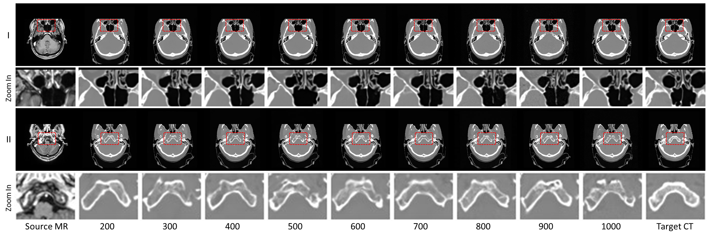
Figure 6: Visual comparison between images generated using different amount of low-frequency information (numbers of forward diffusion steps $\tilde{T}$).

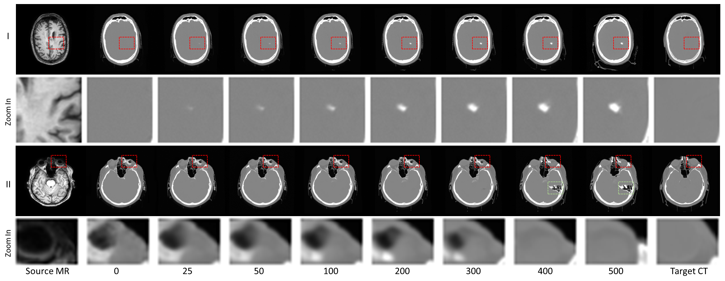
Figure 7: Visual comparison between images generated using different $\overline{T}$ steps at which the high-frequency information conditioning was dropped.

References

- Armanious et al. [2020] Karim Armanious, Chenming Jiang, Marc Fischer, Thomas Küstner, Tobias Hepp, Konstantin Nikolaou, Sergios Gatidis, and Bin Yang. Medgan: Medical image translation using gans. Computerized medical imaging and graphics, 79:101684, 2020.
- Chandarana et al. [2018] Hersh Chandarana, Hesheng Wang, RHN Tijssen, and Indra J Das. Emerging role of mri in radiation therapy. Journal of Magnetic Resonance Imaging, 48(6):1468–1478, 2018.
- Dhariwal and Nichol [2021] Prafulla Dhariwal and Alexander Nichol. Diffusion models beat gans on image synthesis. Advances in Neural Information Processing Systems, 34:8780–8794, 2021.
- Edmund and Nyholm [2017] Jens M Edmund and Tufve Nyholm. A review of substitute ct generation for mri-only radiation therapy. Radiation Oncology, 12:1–15, 2017.
- Fu et al. [2019] Huan Fu, Mingming Gong, Chaohui Wang, Kayhan Batmanghelich, Kun Zhang, and Dacheng Tao. Geometry-consistent generative adversarial networks for one-sided unsupervised domain mapping. In Proceedings of the IEEE/CVF Conference on Computer Vision and Pattern Recognition, pages 2427–2436, 2019.
- Goitein et al. [1979] Michael Goitein, Jack Wittenberg, Marta Mendiondo, Joanne Doucette, Carl Friedberg, Joseph Ferrucci, Leonard Gunderson, Rita Linggood, William U Shipley, and Harvey V Fineberg. The value of ct scanning in radiation therapy treatment planning: a prospective study. International Journal of Radiation Oncology* Biology* Physics, 5(10):1787–1798, 1979.
- Goodfellow et al. [2020] Ian Goodfellow, Jean Pouget-Abadie, Mehdi Mirza, Bing Xu, David Warde-Farley, Sherjil Ozair, Aaron Courville, and Yoshua Bengio. Generative adversarial networks. Communications of the ACM, 63(11):139–144, 2020.
- Heusel et al. [2017] Martin Heusel, Hubert Ramsauer, Thomas Unterthiner, Bernhard Nessler, and Sepp Hochreiter. Gans trained by a two time-scale update rule converge to a local nash equilibrium. Advances in neural information processing systems, 30, 2017.
- Ho et al. [2020] Jonathan Ho, Ajay Jain, and Pieter Abbeel. Denoising diffusion probabilistic models. Advances in Neural Information Processing Systems, 33:6840–6851, 2020.
- Huang et al. [2018] Xun Huang, Ming-Yu Liu, Serge Belongie, and Jan Kautz. Multimodal unsupervised image-to-image translation. In Proceedings of the European conference on computer vision (ECCV), pages 172–189, 2018.
- Kaji and Kida [2019] Shizuo Kaji and Satoshi Kida. Overview of image-to-image translation by use of deep neural networks: denoising, super-resolution, modality conversion, and reconstruction in medical imaging. Radiological physics and technology, 12(3):235–248, 2019.
- Kazemifar et al. [2019] Samaneh Kazemifar, Sarah McGuire, Robert Timmerman, Zabi Wardak, Dan Nguyen, Yang Park, Steve Jiang, and Amir Owrangi. Mri-only brain radiotherapy: Assessing the dosimetric accuracy of synthetic ct images generated using a deep learning approach. Radiotherapy and Oncology, 136:56–63, 2019.
- Kingma et al. [2019] Diederik P Kingma, Max Welling, et al. An introduction to variational autoencoders. Foundations and Trends® in Machine Learning, 12(4):307–392, 2019.
- Kong et al. [2021] Lingke Kong, Chenyu Lian, Detian Huang, Yanle Hu, Qichao Zhou, et al. Breaking the dilemma of medical image-to-image translation. Advances in Neural Information Processing Systems, 34:1964–1978, 2021.
- Li et al. [2023] Yunxiang Li, Hua-Chieh Shao, Xiao Liang, Liyuan Chen, Ruiqi Li, Steve Jiang, Jing Wang, and You Zhang. Zero-shot medical image translation via frequency-guided diffusion models. IEEE transactions on medical imaging, 2023.
- Liu et al. [2017] Ming-Yu Liu, Thomas Breuel, and Jan Kautz. Unsupervised image-to-image translation networks. Advances in neural information processing systems, 30, 2017.
- Meng et al. [2021] Chenlin Meng, Yang Song, Jiaming Song, Jiajun Wu, Jun-Yan Zhu, and Stefano Ermon. Sdedit: Image synthesis and editing with stochastic differential equations. arXiv preprint arXiv:2108.01073, 2021.
- Özbey et al. [2023] Muzaffer Özbey, Onat Dalmaz, Salman UH Dar, Hasan A Bedel, Şaban Özturk, Alper Güngör, and Tolga Çukur. Unsupervised medical image translation with adversarial diffusion models. IEEE Transactions on Medical Imaging, 2023.
- Payne and Leach [2006] GS Payne and MO Leach. Applications of magnetic resonance spectroscopy in radiotherapy treatment planning. The British journal of radiology, 79(special_issue_1):S16–S26, 2006.
- Saw et al. [2005] Cheng B Saw, Alphonse Loper, Krishna Komanduri, Tony Combine, Saiful Huq, and Carol Scicutella. Determination of ct-to-density conversion relationship for image-based treatment planning systems. Medical Dosimetry, 30(3):145–148, 2005.
- [21] Hua-Chieh Shao, Yunxiang Li, Jing Wang, Steve Jiang, and You Zhang. Real-time liver motion estimation via deep learning-based angle-agnostic x-ray imaging. Medical physics.
- Shao et al. [2023] Hua-Chieh Shao, Yunxiang Li, Jing Wang, Steve Jiang, and You Zhang. Real-time liver tumor localization via combined surface imaging and a single x-ray projection. Physics in Medicine & Biology, 68(6):065002, 2023.
- Sohl-Dickstein et al. [2015] Jascha Sohl-Dickstein, Eric Weiss, Niru Maheswaranathan, and Surya Ganguli. Deep unsupervised learning using nonequilibrium thermodynamics. In International Conference on Machine Learning, pages 2256–2265. PMLR, 2015.
- Song et al. [2021a] Jiaming Song, Chenlin Meng, and Stefano Ermon. Denoising diffusion implicit models. In International Conference on Learning Representations, 2021a.
- Song et al. [2021b] Yang Song, Jascha Sohl-Dickstein, Diederik P Kingma, Abhishek Kumar, Stefano Ermon, and Ben Poole. Score-based generative modeling through stochastic differential equations. In International Conference on Learning Representations, 2021b.
- Thornton Jr et al. [1992] AF Thornton Jr, HM Sandler, RK Ten Haken, DL McShan, BA Fraass, ML LaVigne, and BR Yanks. The clinical utility of magnetic resonance imaging in 3-dimensional treatment planning of brain neoplasms. International Journal of Radiation Oncology* Biology* Physics, 24(4):767–775, 1992.
- Wang et al. [2022] Kai Wang, Yunxiang Li, Michael Dohopolski, Tao Peng, Weiguo Lu, You Zhang, and Jing Wang. Recurrence-free survival prediction under the guidance of automatic gross tumor volume segmentation for head and neck cancers. In 3D Head and Neck Tumor Segmentation in PET/CT Challenge, pages 144–153. Springer, 2022.
- Yang et al. [2022] Ling Yang, Zhilong Zhang, Yang Song, Shenda Hong, Runsheng Xu, Yue Zhao, Yingxia Shao, Wentao Zhang, Bin Cui, and Ming-Hsuan Yang. Diffusion models: A comprehensive survey of methods and applications. arXiv preprint arXiv:2209.00796, 2022.
- Zhang et al. [2023] Yifan Zhang, Fan Ye, Lingxiao Chen, Feng Xu, Xiaodiao Chen, Hongkun Wu, Mingguo Cao, Yunxiang Li, Yaqi Wang, and Xingru Huang. Children’s dental panoramic radiographs dataset for caries segmentation and dental disease detection. Scientific Data, 10(1):380, 2023.
- Zhao et al. [2022] Min Zhao, Fan Bao, Chongxuan Li, and Jun Zhu. Egsde: Unpaired image-to-image translation via energy-guided stochastic differential equations. arXiv preprint arXiv:2207.06635, 2022.
- Zhu et al. [2017] Jun-Yan Zhu, Taesung Park, Phillip Isola, and Alexei A Efros. Unpaired image-to-image translation using cycle-consistent adversarial networks. In Proceedings of the IEEE international conference on computer vision, pages 2223–2232, 2017.