Security Fence Inspection at Airports Using Object Detection

Nils Friederich¹ Andreas Specker^3,4 Jürgen Beyerer^3,2,4
¹Karlsruhe Institute of Technology, Institute for Automation and Applied Informatics
²Karlsruhe Institute of Technology, Institute for Anthropomatics and Robotics
³Fraunhofer IOSB ⁴Fraunhofer Center for Machine Learning
nils.friederich@kit.edu {andreas.specker,juergen.beyerer}@iosb.fraunhofer.de

Abstract

To ensure the security of airports, it is essential to protect the airside from unauthorized access. For this purpose, security fences are commonly used, but they require regular inspection to detect damages. However, due to the growing shortage of human specialists and the large manual effort, there is the need for automated methods. The aim is to automatically inspect the fence for damage with the help of an autonomous robot. In this work, we explore object detection methods to address the fence inspection task and localize various types of damages. In addition to evaluating four State-of-the-Art (SOTA) object detection models, we analyze the impact of several design criteria, aiming at adapting to the task-specific challenges. This includes contrast adjustment, optimization of hyperparameters, and utilization of modern backbones. The experimental results indicate that our optimized You Only Look Once v5 (YOLOv5) model achieves the highest accuracy of the four methods with an increase of 6.9% points in Average Precision (AP) compared to the baseline. Moreover, we show the real-time capability of the model. The trained models are published on GitHub: https://github.com/N-Friederich/airport_fence_inspection.

1 Introduction

In contemporary times, airplanes have assumed a crucial role in global transportation. Ensuring the safety of passengers, cargo, and machinery is of great importance. This requires appropriate safety mechanisms, both onboard the aircraft and within the airport infrastructure. Protecting sensitive areas such as the airside is a major challenge for airport operators. In Germany, for instance, there are over 540 airfields, out of which 15 are classified as international airports according to § 27d Paragraph 1 Luftverkehrsgesetz (LuftVG) ¹¹1https://www.gesetze-im-internet.de/ (Gesetz im Netz - Federal Ministry of Justice), Date 01/09/2023 [dfs_statistik]. To obtain this classification, airfields must secure their sensitive areas, including the airside, against unauthorized access by adhering to § 8 Luftsicherheitsgesetz (LuftSiG) 1. Appropriate security fences are a common practice to protect these areas [easa_cs_adr_dsn]. These fences must be regularly checked for damage in accordance with § 8 and § 9 LuftSiG 1. Even minor damage to the fence potentially allows animals to enter the airfield and pose a danger to themselves, people, and machinery [easa_cs_adr_dsn]. However, the availability of skilled human personnel to perform fence inspections is becoming increasingly limited [Burstedde2022Fachkr]. Therefore, exploring automated methods to monitor this real-world surveillance application, such as utilizing mobile robots with cameras for detecting damages, is highly valuable.

Refer to caption — Figure 1: Examples of damaged security fences – The BBox colors symbolize different types of damage: Green marks a hole in the fence; Red marks damage to the climb-over-protection.

To implement such an automatic system, this work focuses on 2D object detection methods for three main reasons. First, the existing literature offers numerous robust methods to effectively tackle this task [yolov5, tood, varifocalnet, mmdetection]. Second, using cheap camera sensors is adequate for capturing the necessary imagery. Last, 2D image processing is computationally less heavy compared to, e.g., processing 3D data from a stereo camera.

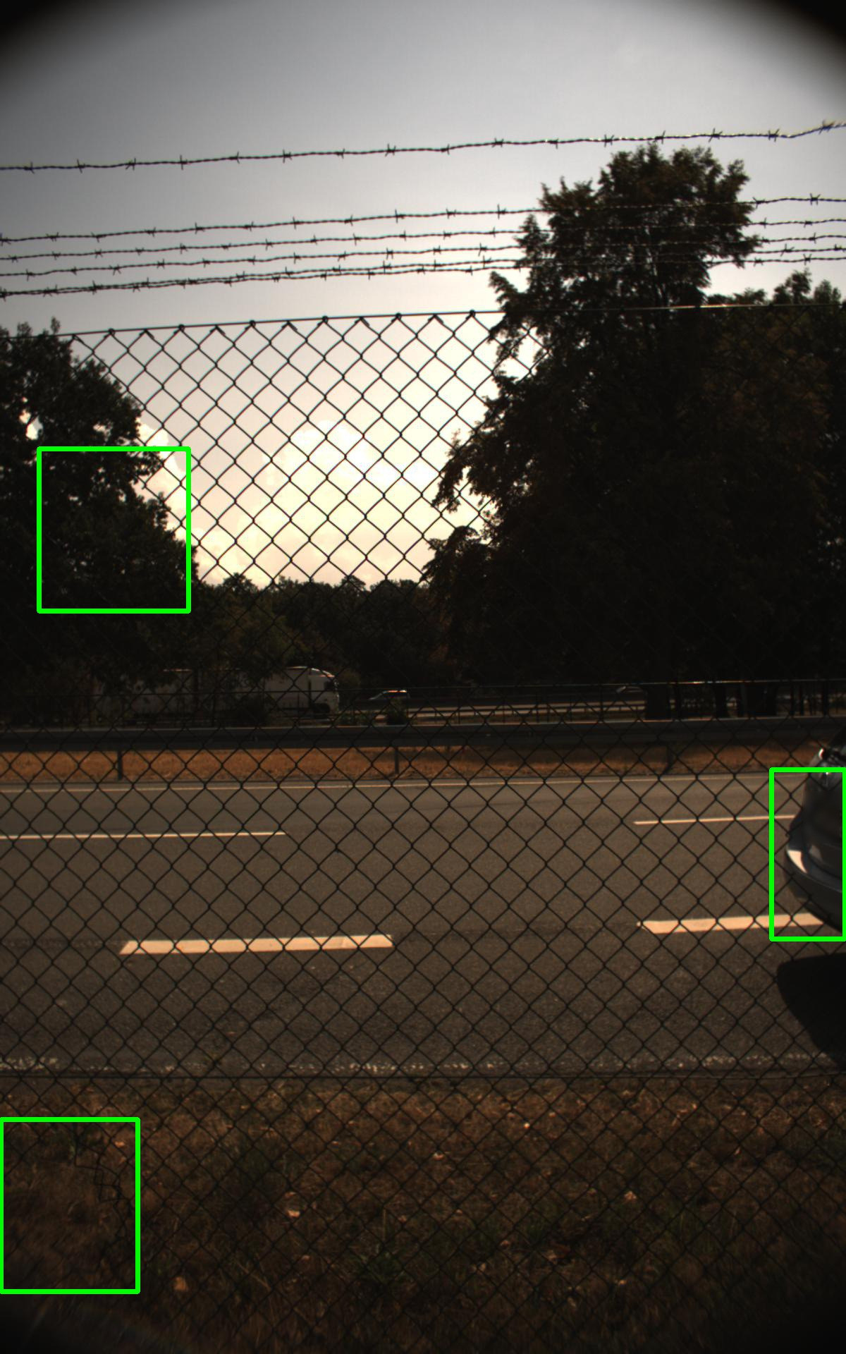
In general, object detection methods aim at identifying and localizing specific objects or patterns within an input image. In the context of this work, our objective is to detect two commonly occurring types of damages within fence images captured at airports using a self-recorded dataset. Two examples of airport fences are presented in Fig. 1. There is a wire mesh structure in the lower part as a passage barrier and multiple rows of barbed wire in the upper part for climbing-over protection. Damage can occur in both sections. However, damage detection needs a clear differentiation between the fence and structures in the background. Moderate contrast in many areas, such as with the trees in the background, hardens the task. In addition, background clutter, e.g., leaves, further complicates the detection process, especially with the intricate wire mesh. To overcome these challenges, various techniques, including contrast adjustment, are examined throughout this work. For this purpose, SOTA deep learning methods, namely YOLOv5 [yolov5], Task-aligned One-stage Object Detection (TOOD) [tood], VarifocalNet (VFNet) [varifocalnet], and Deformable DEtetction TRansformer (DETR) [deformable_detr], are evaluated and compared for their potential in addressing the detection challenges associated with the security fence inspection task. Ideally, the resulting detection system should work autonomously on a mobile robot. However, this requires the most economical operation possible with reliable damage detection on affordable hardware. Therefore, we also investigate the tradeoff between speed and accuracy.

In summary, the main contributions of this paper are threefold:

•

We conduct the first analysis of SOTA object detection methods for the security fence inspection use case.
•

Our thorough evaluation of various design choices highlights key factors for strong damage detection results.
•

The resulting real-time model demonstrates remarkable performance and generalization ability and, thus, provides a strong baseline for future research.

2 Related Work

The automated damage detection at airport fences requires Computer Vision (CV) algorithms [cv_algos_hw_impl_survey]. In this use case, a simple image classification approach would be insufficient, resulting in a time-consuming search game for human operators. On the other hand, precise segmentation is not required for this task, as it does not demand detailed segmentation of each object instance wire. In addition, creating segmentation labels for intricate objects such as the wire mesh structure by human annotators would be both time-consuming and costly [pixel_label_fine_segm]. Therefore, object detection is utilized as a compromise between classification and segmentation. For the purpose of object detection, Deep Learning (DL) methods have gained prominence over classical CV methods due to hierarchical feature extraction, higher accuracy, and improved generalization capabilities [feature_extraction_ir_cv, dl_vs_tradCV, dl_cv_brief_review, review_dl_material_degradation]. For object detection methods, a differentiation can be made between anchor-based and anchor-free methods. Whereas anchor-based methods often converge faster, anchor-free methods require fewer hyperparameters and may have stronger generalization capabilities. Whether this is true in the context of this thesis is evaluated using the anchor-based method YOLOv5 and the anchor-free methods TOOD, VFNet and Deformable DETR.

Regardless of the model type, DL models often encounter issues with overfitting, particularly when dealing with small datasets. To mitigate this issue, pre-trained models are commonly employed. Since no pre-trained model tailored explicitly for the use case has been published, a default pre-trained model is utilized, such as those trained on the Common Objects in Contexts (COCO) dataset [coco_map, survey_tran_learn]. Furthermore, to the best of our knowledge, no appropriate datasets for security fence inspection have been published. Although there are related use cases, such as de-fencing [stream_img_defencing_smartphones, defencing_sing_img_dcnn, robust_effizient_defencing_cgan], these datasets consist of images taken in closer proximity and different spatial contexts [robust_effizient_defencing_cgan].

3 Methodology

This paper thoroughly examines the use of SOTA DL methods with different characteristics regarding their suitability for the damage detection task and derives best practices concerning design criteria. In detail, YOLOv5 [yolov5], TOOD [tood], VFNet [varifocalnet], and Deformable DETR [deformable_detr] are considered. After motivating these choices in Sec. 3.1, several adaptions are introduced to increase the detection performance for the task under real-world conditions. The overall goal is to identify the best design characteristics for DL methods from a quantitative perspective and further investigate this method concerning the influence of input image resolution to achieve a beneficial trade-off between detection results and computational complexity.

3.1 Deep Learning Methods

Recently, numerous new DL methods have been introduced [yolov5, tood, varifocalnet, ddod, detr, deformable_detr]. In terms of real-time object detection, several derivatives of the YOLO approach [yolov3v4v5_auto_brunch_det, yolov3v4v5_autonom_faulty_uavs, yolov3v4v5_paultry_recognition, yolov5_face_recog] have proven suitable for various real-world applications [yolov5_safty_helmet_det, yolov5_face_mask]. For instance, YOLOv5 achieves good detection results at lower operational expenses. However, YOLOv5 and its predecessors [yolo9000, yolov3, yolov4] are anchor-based, which may lead to limitations in generalization capabilities [analysis_anchorbased_anchorfree_od_dl]. Therefore, two anchor-free DL methods are included in the analysis, namely TOOD [tood] and VFNet [varifocalnet].

All these three methods were developed as CNN-based methods [tood, varifocalnet, yolov5]. Since transformer-based models promise improved generalization capabilities [cnn_vs_vit], the transformer-based Deformable DETR [deformable_detr], a successor of the popular Vision Transformer (ViT)-based DETR [detr], is investigated. However, Transformers, such as ViT, typically require more training data than Convolutional Neural Networks (CNNs) [scale_vision_transformer]. Since the available data for the fence inspection task is limited, further investigations need to be conducted.

3.2 Optimizations

In this work, we thoroughly study various design parameters to improve damage detection in security fences under real-world settings. In the following, the considered aspects are motivated and introduced.

Numerical stability: When implementing DL methods, numerical instabilities such as exploding gradients or zero divisions may occur. These numerical instabilities can lead to a degradation of the training results, which is why we eliminate them to improve the meaningfulness of the experiments. We contributed our code changes to the original code repositories.

Regularization: Regularization of DL models is crucial for preventing overfitting on small datasets with few Regions of Interest (RoIs) per image. For this, primarily three adaptations are investigated. First, the image weighting technique from YOLOv5 is used to over-represent difficult training examples. Due to the small training dataset, edge cases that occur rarely may otherwise be covered by the background noise of decent images. Second, optimizers with regularization abilities like Adam [adam] or AdamW [adamW] are investigated. To prevent gradient oscillations but at the same time allow for a steep gradient descent, the impact of learning rate adjustments is explored.

Data augmentation: Data augmentation methods aim at increasing the diversity in small-scale datasets to prevent overfitting and improve robustness. Due to the small amount of data with few damages each, the impact of data augmentation methods like mosaic and affine transformations are investigated.

Contrast enhancement: Poor contrast, e.g., caused by low light during dusk or dawn, presents a significant challenge in detecting damages on airport fences. In such cases, the fine structures of the fences do not stand out clearly against the background. Pre-processing images with contrast enhancement methods prior to damage detection alleviates the problem. Contrast adjustment can generally be executed on the entire image or separately for multiple image regions. We compare both global and local contrast enhancement methods represented by Histogram equalization (HistEqu) [comprehensive_survey_img_contrast_techniques, survey_img_enhancement_tequ] and Contrast Limited Adaptive Histogram Equalization (CLAHE) [clahe], respectively.

Backbone: While YOLOv5 utilizes a modern CSPDarknet [yolov4_scaled, cspnet] as backbone [yolov5], TOOD and VFNet rely on variants of the Residual Network (ResNet) [resnet] and ResNeXt [resnext] architectures. However, more recent backbones such as Res2Net [res2net] or ConvNeXt [convNeXt] show better performance in various tasks [convnext_yolo, convnext_unet]. Therefore, these backbones are applied in conjunction with TOOD and VFNet. Analogous to the original backbones, we pre-train these backbones on the COCO dataset first.

Hyperparameter tuning: The choice of appropriate hyperparameters is essential to assure good performance, especially if few training data are available. In addition, the fence inspection task requires strong generalization capabilities. Due to the different conditions and demands, hyperparameters proposed by the original works might not be optimal in damage detection. As a result, detailed studies concerning the choice of hyperparameters are conducted.

Image resolution: When object detectors are deployed in real-world applications, fast computation is crucial. For instance, if the processing is performed on autonomous platforms, such as robots. The inference speed of object detectors is greatly affected by the resolution of the input images. Higher-resolution images provide a more detailed context, enabling improved detection of damages, while the computational complexity increases. Thus, achieving a suitable trade-off between detection accuracy and computational requirements is essential.

4 Experiments

For maximum reproducibility, the hardware and software stack was kept constant during all experiments. The official implementations of YOLOv5 (v6.2) [yolov5] and MMDetection (MMDet) (v2.25.1) [mmdetection] were used as the basis for our adaptions and experiments. The methods were then executed using Nvidia’s A6000 GPU and Intel’s Xeon Silver 4210R CPU.

4.1 Dataset & Evaluation Metrics

Since there is no publicly available dataset for the task, a dataset of airport fence damages was created. Therefore, video sequences of different sections were recorded using two different camera models, namely a FLIR²²2flir.eu, Date: 01/09/2023 camera model and Panasonic’s GH5³³3panasonic.com, Date: 01/09/2023. A total of 5 datasets were recorded, 3 with the FLIR and 2 with the GH5 camera. Then all images with damage were labeled, images without damage were sorted out and were not considered further. This results in 5 video sequences with an overall 475 video frames and 725 annotated damages, divided into 104 climb-over defects and 621 holes. The images recorded with the FLIR camera have a resolution of $1920\times 1200$ and those with the GH5 camera of $1920\times 1080$ , respectively.

Case	Training	Validation	Test
1	FLIR	FLIR	FLIR
2	FLIR	FLIR	GH5
3	FLIR+GH5	FLIR+GH5	FLIR+GH5

Table 1: Dataset splits – Each investigation case specifies which the datasets used for training, validation, and testing. Training and evaluation are performed in each examination case according to the LOOCV.

This work considers three different cases, each reflecting another real-world scenario. The cases differ regarding the training, validation, and testing data, as shown in Tab. 1. Case 1 is the specialization case when training data from the exact camera used in the application is available. Case 2 evaluates the generalization performance since training and test data originate from different camera models with dissimilar characteristics. In the last Case 3, data from both camera models are used for all splits to evaluate the case when diverse data is available for training.

To ensure meaningful evaluation results, Leave-One-Out Cross-Validation (LOOCV)is performed in each of the three study cases to compensate for the small size of the dataset. In each split, another video sequence is leveraged for training, resulting in 12 splits.

The COCO AP [coco_map] serves as the primary metric for both evaluation and validation. The results given represent the average across all three cases and will be abbreviated as Avg. AP in the following.

4.2 Baseline

Each method’s baseline is evaluated on the 12 Leave-One-Out Cross-Validation (LOOCV) splits. For this purpose, the original implementations of the methods were slightly modified. For YOLOv5, only Pytorch’s recommended measures for reproducibility⁴⁴4pytorch.org, Date 01/09/2023 were added. This ensures better comparability of experiments. Unfortunately, this was impossible for the other three methods in MMDet 2.25.1. Nevertheless, to reduce the standard deviation between the training runs and to be able to make more meaningful comparisons, three runs were performed for each data split. For training, four changes were made to the original configurations. First, the batch size was reduced from 32 to 8 to allow a training with faster gradient descent. Second, to reduce the oscillation of the metrics validation curve during training, the learning rate was reduced to 5e-2. Third, the number of epochs had to be doubled for training convergence. Fourth and last, FP16 built-in training for faster training and lower memory consumption is used.

For all models, pre-trained COCO models are utilized. The models were then fine-tuned with the fence inspection dataset, whereby the resolution was adjusted to 768 pixels on the longest image side. Tab. 2 provides the baseline results of the four methods.

Method	Backbone	Avg.	Case 2
Method	Backbone	AP	AP
YOLOv5 [yolov5]	n6	53.52 $\pm$ 21	25.86 $\pm$ 8
	s6	55.33 $\pm$ 21	27.42 $\pm$ 7
	m6	59.53 $\pm$ 17	37.44 $\pm$ 2
	l6	61.37 $\pm$ 15	41.84 $\pm$ 4
	x6	62.19 $\pm$ 14	43.34 $\pm$ 0
TOOD [tood]	ResNet 50	66.14 $\pm$ 11	50.42 $\pm$ 2
	ResNet 101	67.03 $\pm$ 12	51.95 $\pm$ 4
	ResNeXt101-64x4d	67.10 $\pm$ 12	50.84 $\pm$ 2
VFNet [varifocalnet]	ResNet 50	65.64 $\pm$ 14	47.22 $\pm$ 3
	ResNet 101	65.78 $\pm$ 13	47.86 $\pm$ 2
	ResNeXt101-64x4d	67.75 $\pm$ 12	50.28 $\pm$ 3
Def. DETR [deformable_detr]	ResNet 50	61.13 $\pm$ 14	42.11 $\pm$ 5

Table 2: Baseline results – Different backbone configurations for each method are compared. For TOOD and VFNet, all configs use DConvs [dcn, dcnv2] and Multi-Scaling as additional data augmentation strategy. The best result for each configuration is highlighted in bold.

The results indicate that TOOD and VFNet provide the best results with 67.10% and AP 67.75% AP. YOLOv5 achieves worse outcomes with 62.19% AP, though still surpassing Deformable DETR by 2.06% points. One reason for the poor accuracy of Deformable DETR could be the limited training data, a general problem with transformers. Since the efficiency of Deformable DETR is significantly worse than YOLOv5 due to its transformer-based construction, the Deformable DETR method is not considered further in the remainder of this paper. One reason for the poorer results of YOLOv5 is the subpar generalization capability. Comparing the results for Case 2 in Tab. 2, it is apparent that the anchor-free TOOD and VFNet methods generalize remarkably stronger to unseen data. Whether this weakness of YOLOv5 remains despite the optimizations in the further chapters is investigated in Sec. 4.6.

4.3 Regularization

After training the baseline, optimizations are made for the three remaining methods. We have adjusted the YOLOv5 implementation to enable training with rectangular images training in conjunction with random shuffling and mosaic data augmentation [yolov5]. Furthermore, different hyperparameter settings proved beneficial for the m6, l6, and x6 variants of YOLOv5 to achieve better convergence toward the global optimum and prevent overfitting. On the one hand, the OneCycle learning rate [onecyclelr] is increased from 1e-4 to 1e-3 to enable faster convergence of the deeper models m6, l6 and x6 and better exploit the hill climbing properties in gradient optimization. Second, more data augmentation is employed for enhanced regularization. For this, the percentage of image scaling is increased from $[-50\%,+50\%]$ to $[-90\%,+90\%]$ . In addition, MixUp [mixup] is applied with a probability of 10%. Regarding TOOD and VFNet, no significant enhancements were observed.

Backbone	Params	FLOPs	Avg.
	$(M)$	$(B)$	AP
n6	3.2	4.7	60.71 $\pm$ 18
s6	12.6	17	62.36 $\pm$ 15
m6	35.7	50.3	64.68 $\pm$ 14
l6	76.8	111.8	66.05 $\pm$ 14
x6	140.7	210.5	64.85 $\pm$ 14

Table 3: YOLOv5 baseline optimization results – The best result is highlighted in bold.

The optimized YOLOv5 results are presented in Tab. 3. The results significantly surpass the baseline results. This is attributed to the increased diversity of data during training through Mosaic Data Augmentation and further regularization against overfitting introduced by shuffling. In total, these adjustments resulted in an improvement of 3.86% points in AP when comparing the best configurations. However, the best model is not the largest x6, but l6. The x6 model tends to overfit and performs notably worse with 64.85% AP. Even the increased data augmentation and additional regularization cannot compensate for this. Therefore, YOLOv5 l6 is used as the best model in the following.

4.4 Contrast Adjustment

Method	Experiment	Avg.	Case 1	Case 2	Case 3
Method	Experiment	AP	AP	AP	AP
YOLOv5 [yolov5]	Regularization	66.05 $\pm$ 14	73.45 $\pm$ 4	47.74 $\pm$ 4	76.97 $\pm$ 2
	CLAHE	66.22 $\pm$ 14	73.87 $\pm$ 3	47.28 $\pm$ 1	77.51 $\pm$ 2
	HistEqu	67.16 $\pm$ 14	75.46 $\pm$ 4	48.88 $\pm$ 2	77.14 $\pm$ 2
TOOD [tood]	Baseline	67.10 $\pm$ 12	73.24 $\pm$ 4	50.84 $\pm$ 2	77.24 $\pm$ 2
	CLAHE	64.52 $\pm$ 14	72.07 $\pm$ 4	45.86 $\pm$ 5	75.63 $\pm$ 3
	HistEqu	67.62 $\pm$ 11	73.33 $\pm$ 4	52.31 $\pm$ 1	77.22 $\pm$ 2
VFNet [varifocalnet]	Baseline	67.75 $\pm$ 12	74.14 $\pm$ 2	50.87 $\pm$ 3	78.25 $\pm$ 2
	CLAHE	65.14 $\pm$ 15	72.97 $\pm$ 3	44.54 $\pm$ 3	77.91 $\pm$ 2
	HistEqu	67.49 $\pm$ 13	73.73 $\pm$ 2	50.40 $\pm$ 3	78.36 $\pm$ 2

Table 4: HistEqu and CLAHE results – Results obtained with the best configuration of methods. The first line of each block indicates the best experiments so far on the original dataset. For comparison, the best results of YOLOv5 were taken from Sec. 4.3 and for TOOD and VFNet from Sec. 4.2. The best results for each DL method are highlighted in bold.

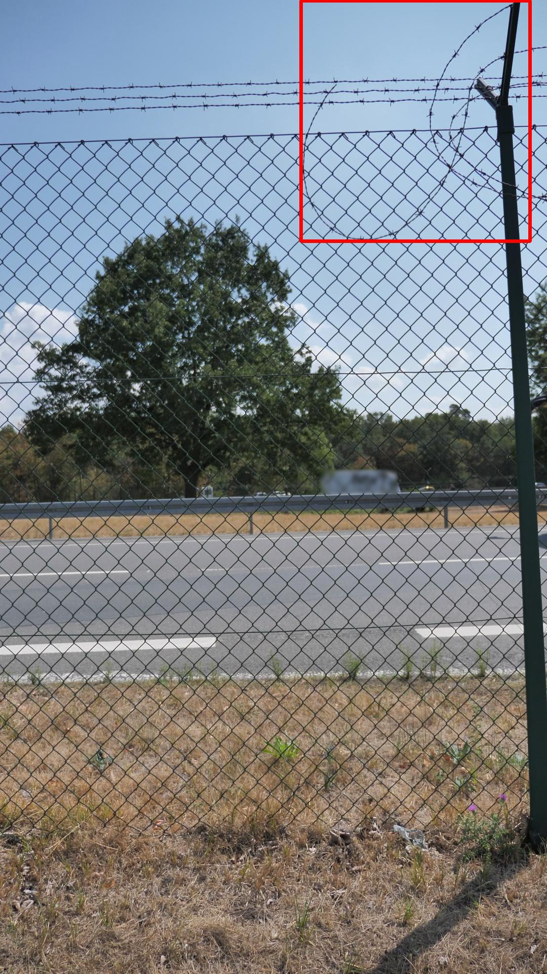
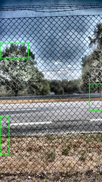
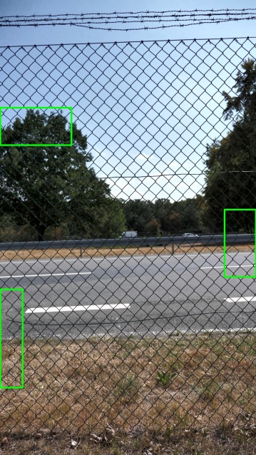
The two contrast adjustment methods CLAHE and HistEqu are compared in Tab. 4. The results indicate superior performance of the global method HistEqu regardless of the detection approach. One reason for this could be the over-adjustment of CLAHE in certain regions. Especially worse results concerning the generalization Case 2 support this hypothesis. Since GH5 images already show good contrast, an additional contrast adjustment leads to over-adjustment. Fig. 2 visualizes the differences between both methods for an image captured by the GH5 camera. The CLAHE method, as shown in Fig. 2(b), clearly over-adjusts, compared to HistEqu, which is depicted in Fig. 2(c). These overfits occur in areas with a high difference between light and dark pixels, such as trees and the sky. This leads to a very unnatural appearance of the image. As a result, parts of the fence structure are hardly recognizable.

4.5 Hyperparameter Optimization

The hyperparameters are optimized using HistEqu preprocessing. Analogous to regularization, the MMDet implementation methods TOOD and VFNet provide no significantly improved results. As a result, hyperparameter optimization focuses on YOLOv5. We found that choosing a learning rate of 5e-3 and applying image weighting turned out to be beneficial. This manual hyperparameter optimization increases the AP from 67.16% to 68.45%. Besides, numerous settings freezing different stages of the backbone, and the use of Adam [adam] and AdamW [adamW] as the optimizer were evaluated to achieve stronger regularization and thereby a more stable training. We also evaluated several settings regarding the affine transformations to achieve a higher generalization. However, none of the mentioned adjustments led to significantly improved results.

Thereafter, an automatic hyperparameter tuning was performed. First, all previous internal evaluations of all 12 LOOCV splits were used, and the Pearson Correlation Coefficient between the average AP across the splits and the AP of each individual split was determined. Subsequently, the split is identified that correlates most with the average AP over all splits. This split is leveraged for automatic hyperparameter tuning.

We apply the Genetic Algorithm (GA) [genetic_algo_ai] implemented in YOLOv5 for automatic hyperparameter optimization in the predefined configuration, except for a few changes. Based on our previous findings, we reduce the defined search space and exclude the affine transformations rotation, shearing, perspective, and flipping since their use leads to significant degradation. Finally, automatic hyperparameter tuning is executed for 500 iterations with the remaining 21 hyperparameters. In each iteration, one or more hyperparameter adjustments are sampled according to the GA policy and then evaluated in a complete training run without early stopping. The most significant effects were observed in reducing the probability of Mosaic Data Augmentation from 100% to 91.5%, since the network requires original data to capture the inherent structure. Additionally, increasing the variation of the saturation in ColorJitter augmentation from $[-70\%,+70\%]$ to $[-89\%,+89\%]$ lead to notable improvement. In total, the optimized model achieves 69.09% in AP on average across all data splits.

Method	Backbone	DConv	Param	FLOPs	COCO	Avg.
			$(M)$	$(B)$	AP	AP
TOOD	ResNet101	$\times$	53.2	149.0	49.3	67.62 $\pm$ 11
TOOD ⁺	ConvNeXt-T	$\times$	35.7	154.2	44.9	65.86 $\pm$ 13
TOOD	ConvNeXt-T	$\times$	35.7	154.2	48.6	67.76 $\pm$ 12
TOOD	Res2Net101	$\times$	51.7	220.1	45.2	62.05 $\pm$ 9
TOOD	Res2Net101	$\checkmark$	54.5	187.4	50.9	65.13 $\pm$ 9
VFNet	ResNeXt101-32x4d	$\checkmark$	55.1	208.1	49.7	67.49 $\pm$ 13
VFNet ⁺	ConvNeXt-T	$\times$	36.5	161.1	44.5	66.63 $\pm$ 13
VFNet	ConvNeXt-T	$\times$	36.5	161.1	48.9	64.14 $\pm$ 15
VFNet ^*	Res2Net101	$\times$	52.4	227.0	49.2	65.77 $\pm$ 14
VFNet ^*	Res2Net101	$\checkmark$	54.9	187.5	51.1	68.09 $\pm$ 12

Table 5: TOOD and VFNet results with new backbones – In each case, the first line of a block represents the best training so far of the methods from Tab. 4. Best Avg. AP (calculated on our fence dataset) is marked bold.

{}^{*}

Pre-trained weights used.

{}^{+}

Uses original configurations.

4.6 Backbones

After hyperparameter tuning, modern SOTA backbones are evaluated in conjunction with TOOD and VFNet. Besides, the influence of using DConv within the Res2Net architecture is examined. The results of the so-far best models and the new pre-trained ones are given in Tab. 5. For each training session, the AP of the pre-trained network on the COCO dataset is presented in addition to the AP for our dataset. In the case of TOOD, for instance, the best pre-trained network on COCO is not necessarily the best network on our dataset. This is because the classes and the class semantics in the COCO dataset deviate considerably from those in this work. However, it provides a rough indication when further consideration of a backbone is not promising. The findings indicate that TOOD in conjunction with ConvNeXt achieves the highest accuracy. Regarding VFNet, Res2Net as the backbone performs best. Despite the significant improvement in accuracy with the new backbones, TOOD and VFNet do not surpass YOLOv5 in AP. Since YOLOv5 is also more resource efficient due to its design as a real-time object detector, YOLOv5 was selected as the best model and is utilized in the remainder of this paper.

4.7 In-depth Analysis

So far, all analyses have been performed with the AP across all types of failure. This showcased remarkable progress over the baseline with 6.9% points. This section thoroughly delves into the effects of the proposed optimizations to identify strengths and weaknesses of the system.

Damage Type	Metric	YOLOv5		Improvement
Damage Type	Metric	Baseline	Hyp. Opt.	Improvement
All	AP	$62.19\pm 14$	$69.09\pm 12$	+6.90
	$\lx@glossaries@gls@link{main}{ap}{\leavevmode AP}^{small}$	$21.69\pm 14$	$26.80\pm 18$	+5.11
	$\lx@glossaries@gls@link{main}{ap}{\leavevmode AP}^{medium}$	$65.04\pm 11$	$70.75\pm 9$	+5.71
	$\lx@glossaries@gls@link{main}{ap}{\leavevmode AP}^{large}$	$68.52\pm 25$	$83.41\pm 10$	+14.89
Climb over defect	AP	$77.12\pm 12$	$86.53\pm 6$	+9.41
	$\lx@glossaries@gls@link{main}{ap}{\leavevmode AP}^{small}$	$-$	$-$	$-$
	$\lx@glossaries@gls@link{main}{ap}{\leavevmode AP}^{medium}$	$80.80\pm 10$	$89.50\pm 4$	+8.70
	$\lx@glossaries@gls@link{main}{ap}{\leavevmode AP}^{large}$	$77.81\pm 12$	$86.80\pm 6$	+8.99
Hole	AP	$47.26\pm 18$	$51.66\pm 18$	+4.40
	$\lx@glossaries@gls@link{main}{ap}{\leavevmode AP}^{small}$	$21.69\pm 14$	$26.80\pm 18$	+5.11
	$\lx@glossaries@gls@link{main}{ap}{\leavevmode AP}^{medium}$	$50.90\pm 17$	$54.30\pm 18$	+3.40
	$\lx@glossaries@gls@link{main}{ap}{\leavevmode AP}^{large}$	$45.82\pm 41$	$74.88\pm 16$	+29.06

Table 6: Defect results – Comparison between the different types and sizes of damages. Results are given for baseline (see Sec. 4.2) and the Hyp. Opt. (see Sec. 4.5) as the best training of YOLOv5. The different ranges small, medium and large were defined as follows:

0<\lx@glossaries@gls@link{main}{ap}{\leavevmode AP}^{small}\leq

24,000 pixels, 24,000 pixels

<\lx@glossaries@gls@link{main}{ap}{\leavevmode AP}^{medium}\leq

100,000 pixels and 100,000 pixels

<\lx@glossaries@gls@link{main}{ap}{\leavevmode AP}^{large}

Types and area size of fence defects: Tab. 6 investigates the results for each defect type and different sizes of damages for YOLOv5. For this purpose, the damages are divided into three classes based on the covered area in pixels. Damage up to a size of 24,000 pixels is considered small. Correspondingly, damage ranging from 24,000 pixels to 100,000 pixels and over 100,000 pixels as medium or large, respectively. Thereby, 8% of all damages are small, 77% medium and 15% small. In general, the AP difference between the damage types decreases by the optimizations. However, the difference is still a considerable 24.87% points. The stronger detection of the climb-over-protection defects can be explained by their characteristic appearance and by the angle of view. Typically, the damage is in front of the bright sky and, therefore, discriminates well from the background, even under poor lighting conditions (see Fig. 1). In contrast, the wire mesh exhibits poor contrast. The next striking feature in the baseline is the very high standard deviation of 41 for large holes. This finding suggests unstable generalization capabilities and great dependence from the training and validation data. One reason for this is that in the $\lx@glossaries@gls@link{main}{ap}{\leavevmode AP}^{large}$ , the holes are nearly normally distributed up to 500,000 pixels. Therefore, training splits with few large boxes may exceed the generalization capability of the baseline to evaluation splits with huge boxes. The results for the optimized hyperparameters suggest greatly improved generalization capabilities. This improvement contributes to better results over all damages. The detection accuracy for the different damage sizes consistently shows the expected behavior that larger objects are detected more accurately than smaller objects. However, the difference in accuracy is very large in some cases. For instance, the difference for the best model between $AP^{small}$ and $AP^{medium}$ is 35.14% points. Even with a good contrast ratio, small holes caused by, e.g., minor cracks, are difficult to separate from sound parts of the mesh. Interestingly, medium-sized climb over defects are detected more robustly than large ones, regardless of the approach. This is due to a lack of training data depicting large climb over defects. In general, it can be concluded that climb over defects are easier to localize due to their position and larger size. In total, a 34.87% points difference in AP between such damages and holes is observed for the best model.

Metric	YOLOv5		Improvement
Metric	Baseline	Hyp. Opt.	Improvement
Class Error	$0.44\pm 1$	$0.10\pm 0$	$-0.33$
Localization Error	$3.03\pm 3$	$0.80\pm 1$	$-2.23$
As+Localization Error	$0.03\pm 0$	$0\pm 0$	$-0.03$
Duplicate Error	$0.33\pm 0$	$0.26\pm 0$	$-0.07$
Background Error	$0.82\pm 1$	$1.55\pm 2$	$+0.73$
Missing Error	$5.78\pm 5$	$1.44\pm 1$	$-4.34$
False Positive (FP) Rate	$3.79\pm 3$	$4.06\pm 4$	$+0.27$
False Negative (FN) Rate	$7.83\pm 6$	$3.36\pm 3$	$-4.47$

Table 7: YOLOv5 analysis – Comparison of YOLOv5 baseline and optimized results. Metrics are calculated with the TIDE library.

Metric	YOLOv5		Improvement
Metric	Baseline	Hyp. Opt.	Improvement
$\lx@glossaries@gls@link{main}{ap}{\leavevmode AP}^{50}$	$87.52\pm 10$	$91.73\pm 8$	$+4.21$
$\lx@glossaries@gls@link{main}{ap}{\leavevmode AP}^{55}$	$86.47\pm 11$	$90.17\pm 8$	$+3.60$
$\lx@glossaries@gls@link{main}{ap}{\leavevmode AP}^{60}$	$82.47\pm 11$	$87.23\pm 9$	$+4.76$
$AP$