Energizing Federated Learning via Filter-Aware Attention

Abstract

Federated learning (FL) is a promising distributed paradigm, eliminating the need for data sharing but facing challenges from data heterogeneity. Personalized parameter generation through a hypernetwork proves effective, yet existing methods fail to personalize local model structures. This leads to redundant parameters struggling to adapt to diverse data distributions. To address these limitations, we propose FedOFA, utilizing personalized orthogonal filter attention for parameter recalibration. The core is the Two-stream Filter-aware Attention (TFA) module, meticulously designed to extract personalized filter-aware attention maps, incorporating Intra-Filter Attention (IntraFA) and Inter-Filter Attention (InterFA) streams. These streams enhance representation capability and explore optimal implicit structures for local models. Orthogonal regularization minimizes redundancy by averting inter-correlation between filters. Furthermore, we introduce an Attention-Guided Pruning Strategy (AGPS) for communication efficiency. AGPS selectively retains crucial neurons while masking redundant ones, reducing communication costs without performance sacrifice. Importantly, FedOFA operates on the server side, incurring no additional computational cost on the client, making it advantageous in communication-constrained scenarios. Extensive experiments validate superior performance over state-of-the-art approaches, with code availability upon paper acceptance.

1 Introduction

Federated learning (FL) has arisen as a promising distributed learning paradigm that is strategically crafted to mitigate privacy concerns by facilitating collaborative model training among clients without direct data exchange. However, a primary challenge within the FL framework pertains to the issue of data heterogeneity. The presence of disparate data sources with varying characteristics can notably undermine model performance [24].

In conventional FL training, clients collectively strive to train a global shared model [28]. However, the presence of notable data heterogeneity poses a challenge, potentially leading to model degradation upon aggregation [20]. An effective strategy for this issue involves generating personalized parameters for individual client models through a hypernetwork [29]. Despite its efficacy, these methods necessitate a fixed model structure shared among all clients, impeding the personalization of local model structures to accommodate distinct local data characteristics, particularly in heterogeneous client data [8]. Moreover, the generated parameters may exhibit redundancy, lacking the necessary constraints for effective adaptation to specific data distributions. The absence of constraints significantly limits the performance of personalization efforts.

To tackle these challenges, we reconceive the self-attention mechanism  [31] and advocate redirecting attention to the generated filters on the server side, as opposed to recalibrating local model features on the client side. Our novel FL approach is called Federated Orthogonal Filter Attention (FedOFA). Expanding upon the self-attention mechanism, we introduce a Two-Stream Filter-Aware Attention (TFA) module, a key component in FedOFA. TFA posits that boosting personalized performance can be achieved in two filter-aware attention ways: by enhancing the representative capability of individual filters and by exploring relationships between multiple filters to unveil client-specific implicit structures. Concretely, TFA comprises two essential components: Intra-Filter Attention (IntraFA) offers a personalized strategy for selecting critical parameters for individual filters, while Inter-Filter Attention (InterFA) focuses on discovering implicit client-side model structures by establishing connections between different filters. Consequently, TFA can concurrently optimize filters, aligning them with the specific data distribution and enjoying the best of both worlds.

Directly modeling interconnections among all filters in the network proves impractical due to the substantial computational burden associated with the vast parameter count. As a remedy, we propose an approximation approach by investigating layer-wise relationships to alleviate computational overhead. Diverging from self-attention that employs reshaping operations to create patches and multi-heads, we maintain the integrity of individual filters and employ linear projectors to generate diverse multi-heads.

It is crucial to emphasize that TFA diverges markedly from prior self-attention  [31]. Integrating sophisticated attention mechanisms into client-side models demands the refinement of local models, thereby inevitably amplifying computational and communication expenses on the client side. In contrast, the presented TFA functions directly on filters, obviating the requirement for model fine-tuning and incurring no supplementary costs on the client side.

Given the potential redundancy of generated parameters across filters, we propose incorporating orthogonal regularization (OR) within FedOFA to mitigate inter-correlation between filters. This integration of OR ensures that filters maintain orthogonality, promoting diversity and enhancing representation capability.

In the training phase, TFA progressively enforces parameter sparsity by focusing more on pivotal parameters. This inspired the development of an Attention-Guided Pruning Strategy (AGPS) to economize communication expenses. AGPS evaluates the importance of neurons within filters, enabling the tailored customization of models by masking unessential neurons. Diverging from InterFA, AGPS explicitly seeks to explore personalized local architectures, enabling FedOFA to achieve communication efficiency without compromising performance.

Contributions. Our contributions can be summarized as:

• We explore the pivotal role of filters in personalized FL and introduce FedOFA to underscore their significance. Furthermore, we introduce TFA to recalibrate the personalized parameters in a filter-aware way to adapt specific data distribution.

• The proposed FedOFA enriches filter representation capabilities and uncovers implicit client structures without increasing client-side expenses. Furthermore, we furnish a theoretical convergence analysis for our approach.

• We present an attention-guided pruning strategy aimed at mitigating communication overhead by personalizing the customization of local architectures without degrading the performance.

2 Related Works

2.1 Federated Learning

Federated learning, a burgeoning distributed collaborative learning paradigm, is gaining traction for its privacy-preserving attributes, permitting clients to train models without data sharing. A seminal approach, FedAvg [28], necessitates clients to perform local model training, followed by model aggregation on the server. Addressing the constraint of divergent data distributions among clients, several methods have incorporated proximal elements to tackle model drift, exemplified by FedProx [21] and pFedMe [5].

Recent advancements in personalized FL have emerged to tailor global models to specific clients. FedPer [1] aimed to create specific classifiers, sharing some global layers. FedBN [22] alleviated heterogeneity concerns through personalized batch normalization (BN) on the client side. LG-FedAvg [23] integrated a local feature extractor and global output layers into the client-side model. FedKD [35] distilled the knowledge of the global model into local models to enhance personalization performance. Further innovations combined prototype learning with FL [30, 13].

Concurrently, one effective way to achieve personalization is introducing the hypernetwork to generate client-specific models. Jang et al. [14] proposed to use hypernetwork to modulate client-side models for reinforcement learning. Yang et al. [38] explored hypernetworks for customizing local CT imaging models with distinct scanning configurations. Transformer-based personalized learning methods [19] used hypernetworks to generate client-specific self-attention layers. However, this method mandates client-side models to be based on transformers.

Additionally, pFedLA [27] personalized weights in client-side models during aggregation via hypernetworks. Nonetheless, it lacks asynchronous training, requiring clients to participate in every round. FedROD [3] utilized hypernetworks as predictors for local models via distillation loss. Shamsian et al. [29] employed a shared hypernetwork to generate all client-specific model parameters, referred to as pFedHN. Although these methods have demonstrated impressive performance, there remains room for performance improvement and communication efficiency, particularly by focusing on filters and customizing local model structures.

2.2 Attention Mechanism

The attention mechanism emulates human vision, prioritizing salient elements to allocate focus to crucial areas dynamically. Hu et al. [12] introduced channel attention via the squeeze-and-excitation module. Building upon this, Woo et al. [34] amalgamated channel and spatial attention, proposing the convolutional block attention module. Hou et al. [11] incorporated position data into channel attention, naming it coordinate attention. With inspiration from the self-attention mechanism’s success in natural language processing [32], there is a growing interest in integrating self-attention into computer vision. Dosovitskiy et al. [7] demonstrated self-attention’s excellence in image recognition. Swin-transformer [25] extended self-attention with a shifted window.

While self-attention delivers promising outcomes, it focuses on features. This implies that integrating it into FL necessitates additional efforts, such as fine-tuning client-side models and augmenting client-side computational costs.

3 Methodology

Figure 1: The pipeline of the proposed FedOFA. Circles indicate neurons in the filter, with deeper colors indicating higher importance, while white circles are masked neurons.

Figure 2: The proposed FedOFA involves a parameter enhancement process through TFA, comprised of IntraFA and InterFA. IntraFA is dedicated to augmenting the feature representation capacity of individual filters, while InterFA is geared towards uncovering implicit structures. The OR is employed to bolster the diversity of filters. AGPS is used to mask neurons based on their importance ranking selectively. This process serves the dual purpose of achieving personalized model structures and enhancing communication efficiency.

3.1 Overview of FedOFA

The proposed FedOFA operates on the server and focuses on recalibrating filters to adapt specific data distribution. The pipeline of FedOFA is depicted in Fig. 1. Notably, the parameter generation for $i$-th client model is derived from its corresponding embedding vector $\boldsymbol{v}_{i}$ through a hypernetwork. All operations within the FedOFA are executed on the server and directly manipulate the generated parameters of local models. This design offers two significant advantages for implementation: (i) It eliminates the need for fine-tuning hypernetwork architectures and client-side models; and (ii) It avoids incurring additional communicational overhead and client-side computational costs, which is particularly vital in resource-constrained scenarios. FedOFA comprises three main modules: TFA, OR, and AGPS, as illustrated in Fig. 2. In the following, each of these modules will be detailed in the sequel.

3.2 Two-Stream Filter-Aware Attention

In this study, TFA is proposed to enhance filter representation capabilities and uncover personalized implicit structures. However, establishing relationships across the entire network incurs prohibitively high computational costs. Consequently, we propose an approach that approximates network-wide relationships layer-by-layer. Suppose there are $n_{i}$ filters in the $i$-th layer, and $\boldsymbol{C}_{j}^{i}$ denotes the $j$-th in the $i$-th layer. Meanwhile, we concatenate $\{\boldsymbol{C}_{1}^{i},\ldots,\boldsymbol{C}_{n_{i}}^{i}\}$ to present the parameter of $i$-th layer $\boldsymbol{L}^{i}\in\mathbb{R}^{n_{i}\times S_{in}\times k\times k}$, where $S_{in}$ and $k$ correspond to the input channel size, and $k$ denotes the kernel size. Similar to existing self-attention techniques, we initially employ learnable embeddings to transform the input into a high-level semantic feature vector denoted as $\boldsymbol{E}\in\mathbb{R}^{3\times(n_{i}\times S_{in}\times k\times k)}$.

Intra-filter attention. IntraFA is devised to enhance the representation capabilities of filters, necessitating the division of layer-wise embeddings into filter-aware embeddings. For a typical convolutional filter $\boldsymbol{C}\in\mathbb{R}^{S_{in}\times k\times k}$, we perform a split operation on the vector $\boldsymbol{E}$ to obtain individual filter embeddings denoted as $\boldsymbol{E}_{1},...,\boldsymbol{E}_{n_{i}}$. For conciseness, we represent the filter-aware embedding of a single filter as $\boldsymbol{E}_{ra}\in\mathbb{R}^{3\times(S_{in}\times k\times k)}$. Similarly to prior operations, we reshape $\boldsymbol{E}_{ra}$ to derive query, value, and key embeddings, denoted as $\boldsymbol{E}_{ra}^{q},\boldsymbol{E}_{ra}^{k},\boldsymbol{E}_{ra}^{v}$, for the IntraFA stream.

Prior study has demonstrated the effective performance improvement gained through the multi-head mechanism [37]. However, these methods typically implement multi-head mechanisms by reshaping query, key, and value embeddings. This adaptation is necessitated by the computational overhead associated with establishing direct latent relationships between all features. In this work, we strive to preserve the integrity of each convolution filter while harnessing all parameters to uncover latent relationships within each filter. Fortunately, in comparison to feature dimensions, filter dimensions are generally much smaller, enabling us to treat the entire filter as a patch. Therefore, we introduce a linear projection with random initialization to automatically enhance the diversity by generating multiple heads, as formalized below:

$$\boldsymbol{Q}_{ra} =H_{ra}^{Q}(\boldsymbol{E}_{ra}^{q},h),$$ (1)

$$\boldsymbol{K}_{ra} =H_{ra}^{K}(\boldsymbol{E}_{ra}^{k},h),$$ (2)

$$\boldsymbol{V}_{ra} =H_{ra}^{V}(\boldsymbol{E}_{ra}^{v},h),$$ (3)

where $\boldsymbol{Q}_{ra},\boldsymbol{K}_{ra},\boldsymbol{V}_{ra}$ denote the query, key, and value vectors of IntraFA, respectively. $\boldsymbol{Q}_{ra},\boldsymbol{K}_{ra},\boldsymbol{V}_{ra}\in\mathbb{R}^{h\times(S_{in}\times k\times k)}$. $h$ denotes the number of heads. $H_{ra}^{Q}(\cdot,h)$, $H_{ra}^{K}(\cdot,h)$, and $H_{ra}^{V}(\cdot,h)$ represent the linear projections to generate multi-heads for query, key, and value, respectively. After improving the diversity through the multi-head attention mechanism, the attention map can be acquired from:

$$\boldsymbol{Out}_{ra}=Att(\boldsymbol{Q}_{ra}\boldsymbol{K}_{ra})\boldsymbol{V}_{ra},$$ (4)

where $Att(\cdot)$ is the activation function, and the softmax function is used in this paper. A linear projection $P_{ra}(\cdot)$ is used to explore latent relationships among multi-head attention and match the dimension of $C$, which can be formulated as:

$$\boldsymbol{C}_{IntraFA}=\boldsymbol{C}+P_{IntraFA}(\boldsymbol{Out}_{ra}),$$ (5)

where $\boldsymbol{C}_{IntraFA}\in\mathbb{R}^{S_{in}\times k\times k}$ is the recalibrated filter.

Accordingly, IntraFA significantly enhances filter representations by capturing the latent connections among all parameters within each filter. Nonetheless, relying solely on IntraFA is insufficient for uncovering the inter-filter relationships necessary to explore the personalized implicit structures within client-side models.

Inter-filter attention. Existing hypernetwork-based methods generally require fixed local model structures, but the network architecture significantly affects performance, making a shared structure for all clients impractical. Designing personalized structures for diverse clients based on their local data distributions is cost-prohibitive and architecturally challenging. Some methods attempt to weigh different streams to unveil implicit architectures [10] or explore optimal architectures through exhaustive searches [26], suffering from substantial computational costs.

To address these challenges, we introduce InterFA, a method that customizes client-side structures based on exploring the importance of different filters to the specific data. InterFA approximates network-wide relationships by modeling layer-wise relationships. First, we reshape vector $\boldsymbol{E}$ into InterFA’s query, value, and key embeddings, i.e., $\boldsymbol{E}^{q}$, $\boldsymbol{E}^{k}$, and $\boldsymbol{E}^{v}$, where $\boldsymbol{E}^{q},\boldsymbol{E}^{k},\boldsymbol{E}^{v}\in\mathbb{R}^{1\times(n_{i}\times S_{in}\times k\times k)}$.

Like IntraFA, diversity in the embedding vectors is enhanced using $H_{er}^{Q}(\cdot,h)$, $H_{er}^{K}(\cdot,h)$, and $H_{er}^{V}(\cdot,h)$ based on Eqs. (1), (2), and (3). Then, we derive query, key, and value vectors i.e. $\boldsymbol{Q}_{er}$, $\boldsymbol{K}_{er}$, and $\boldsymbol{V}_{er}$, where $\boldsymbol{Q}_{er},\boldsymbol{K}_{er},\boldsymbol{V}_{er}\in\mathbb{R}^{h\times(n_{i}\times S_{in}\times k\times k)}$. Next, Eq. (4) is employed to generate the attention map $\boldsymbol{Out}_{er}$ for InterFA, and then we could obtain the final recalibrated layer $\boldsymbol{L}_{InterFA}$ as follows:

$$\boldsymbol{L}_{InterFA}=\boldsymbol{L}+P_{InterFA}(\boldsymbol{Out}_{er}),$$ (6)

where $P_{InterFA}(\cdot)$ is a linear projection to learn the implicit relationship among multi-head attentions and to match the dimension.

InterFA operates to establish relationships among distinct filters, thus facilitating the exploration of personalized implicit structures to the specific data. It treats each filter as a cohesive patch, preserving its integrity.

IntraFA and InterFA function independently, concentrating on complementary aspects to enhance model performance. Specifically, the $i$-th layer comprising $n_{i}$ filters requires $n_{i}$ IntraFA modules and only one InterFA module. We introduce TFA, where IntraFA and InterFA run as parallel streams to combine both merits. Given the inherent link between enhancing filters and uncovering implicit structures, TFA can potentially optimize performance through joint optimization.

As the value embedding $\boldsymbol{E}^{v}$ characterizes input contents and both streams involve filter-aware attention, we can reshape $\boldsymbol{V}_{ra}$ from $\boldsymbol{V}_{er}$ to reduce computational overhead. The keys and queries operate independently in the two streams for distinct purposes. After enhancing each filter via IntraFA, we concatenate them to obtain the enhanced layer $\boldsymbol{L}_{IntraFA}$. Ultimately, the recalibrated layer is derived through weighted aggregation of the two streams as follows:

$$\boldsymbol{L}_{TFA}=w\boldsymbol{L}_{IntraFA}+(1-w)\boldsymbol{L}_{InterFA},$$ (7)

where $w$ is the weight of IntraFA, which is empirically set to 0.5 in this study.

3.3 Orthogonal Regularization

TFA presents an opportunity to recalibrate the network to the specific data by improving filters and exploring implicit structures. However, it lacks consideration for the independence among filters. To mitigate redundancy and promote filter diversity, OR is introduced [36]. Leveraging orthogonality in linear transformations, OR preserves energy and reduces redundancy in the model’s filter responses [15]. OR employs a penalty function that accounts for orthogonality among filters in each layer with minimal impact on computational complexity.

Specifically, we first reshape the filter responses $\boldsymbol{L}_{TFA}$ into a matrix $\boldsymbol{O}\in\mathbb{R}^{u\times h}$, where $u$ represents the output size, and $h=S_{in}\times k\times k$. The optimization objective for $\boldsymbol{L}$ can be expressed as $\boldsymbol{O}^{\top}\boldsymbol{O}=\boldsymbol{I}$, where $\boldsymbol{I}$ denotes the identity matrix. This formulation aims to enforce orthogonality among filters within each layer, ensuring their maximal independence. $\mathcal{O}$ denotes the set of network weights. Then, OR can be formally defined as:

$$\frac{\lambda}{|\mathcal{O}|}\sum_{\boldsymbol{O}\in\mathcal{O}}\left\|\boldsymbol{O}^{\top}\boldsymbol{O}-I_{h}\right\|_{F}^{2},$$ (8)

where $\lambda$ is the regularization coefficient, which is set to $1e-4$ in this paper. $|\mathcal{O}|$ is the cardinality of $\mathcal{O}$.

To sum up, OR effectively enforces orthogonality among filters, enhancing their diversity and reducing filter redundancy. Consequently, this approach can lead to further improvements in network performance.

3.4 Attention-Guided Pruning Strategy

While InterFA endeavors to uncover implicit structures tailored to various clients, it maintains fixed client-side model structures. Besides, FL often necessitates frequent data transmission between clients and the server, resulting in substantial consumption of communication resources [2, 4]. To address these challenges, we introduce AGPS, capitalizing on TFA’s capacity to zero out unimportant parameters and emphasize critical ones. AGPS customizes the pruning process for unimportant parameters using our attention map to identify an optimal local architecture and promote efficient communication. Initially, AGPS assesses the significance of different neurons and subsequently prunes a specified percentage ($p$%) of them, which can be formulated as:

$$M(cor)=\begin{cases}1,&\text{if ABS}(\boldsymbol{L}_{TFA}(cor))>T\\ 0,&\text{otherwise},\end{cases}$$ (9)

where $\text{ABS}(\cdot)$ denotes the absolute value operation, $T$ represents the value which ranks at $p\%$ in the ascending sorted sequence of $\text{ABS}(\boldsymbol{L}_{TFA})$, and $cor$ is the coordinate index. Finally, we can get the personalized mask $\boldsymbol{M}$.

We mask unimportant parameters, excluding them from the communication process. This operation can be expressed as $\boldsymbol{L}_{TFA}\odot\boldsymbol{M}$, where $\odot$ signifies the element-wise dot product. Consequently, the transmitted neurons are thoughtfully selected to align with the salient aspects of local data, as determined by our filter-aware attention mechanism. This approach effectively represents a neuron-wise pruning strategy for tailoring local structures based on the specific local data, leading to significant reductions in communication costs compared to transmitting all parameters. The pseudo-code of FedOFA is provided in the section of Supplementary Material.

4 Model Analysis

In this section, we propose a theoretical analysis of our methods from two distinct perspectives. Firstly, we establish that our proposed filter-aware attention can be approximated by other feature-aware attention mechanisms. Subsequently, we furnish a proof of convergence for our method.

Let $h(\cdot;\phi)$ be the hypernetwork parameterized by $\phi$, $f(\cdot;\theta_{i})$ represent the $i$-th client-side network parameterized by $\theta_{i}$, and $g(\cdot;\varphi)$ indicate the attention module parameterized by $\varphi$. We denote the training set in the $i$-th client, generated by the distribution $P_{i}$, as $D_{i}=(\boldsymbol{X}_{i},\boldsymbol{y}_{i})$, where $\boldsymbol{X}_{i}$ and $\boldsymbol{y}_{i}$, respectively denote the training samples and their corresponding labels on the $i$-th client.

Relationship to feature-aware attention. For the $i$-th client, the forward process in feature-aware attention can be represented as $g(f(\boldsymbol{x}_{i};\theta_{i});\varphi)$, where $\theta_{i}=h(\boldsymbol{v}_{i};\phi)$. In contrast, our filter-aware attention formulates the forward process as $f(\boldsymbol{x}_{i};g(\theta_{i};\varphi))$. Assuming the hypernetwork and attention modules are linear models, we have $\theta_{i}=\boldsymbol{W}\boldsymbol{v}_{i}$, where $\phi:=\boldsymbol{W}\in\mathbb{R}^{d\times k}$, $\varphi:=\boldsymbol{A}\in\mathbb{R}^{k\times k}$ for filter-aware attention, and $\varphi:=\boldsymbol{A}\in\mathbb{R}^{d\times d}$ for feature-aware attention.

Consistent with the assumption in [29], we further assume $\boldsymbol{X}_{i}^{\top}\boldsymbol{X}_{i}=\boldsymbol{I}$ in this study, which can be achieved through data whitening techniques [9]. In the case of feature-aware attention, we define the empirical risk minimization (ERM) as $\bar{\theta}_{i}=\arg\min_{\theta\in\mathbb{R}^{d}}\left\|\boldsymbol{A}\boldsymbol{X}_{i}\theta-\boldsymbol{y}_{i}\right\|^{2}$, with the optimal solution $\bar{\theta}_{i}=\boldsymbol{X}_{i}^{\top}\boldsymbol{A}^{\top}\boldsymbol{y}_{i}$. Due to OR, $\boldsymbol{A}$ can be optimized over matrices with orthonormal columns, i.e., $\boldsymbol{A}^{\top}\boldsymbol{A}=\boldsymbol{I}$. Then, the ERM can be expressed as:

$$\underset{\theta_{i}}{\arg\min}\left(\boldsymbol{A}\boldsymbol{X}_{i}\theta_{i}-\boldsymbol{y}_{i}\right)^{\top}\left(\boldsymbol{A}\boldsymbol{X}_{i}\theta_{i}-\boldsymbol{y}_{i}\right).$$ (10)

Eq. (10) can be expressed as $\arg\min_{\theta_{i}}\left\|\theta_{i}-\bar{\theta}_{i}\right\|_{2}^{2}$. For the proposed filter-aware attention, the ERM is formulated as $\bar{\theta}_{i}=\arg\min_{\theta\in\mathbb{R}^{d}}\left\|\boldsymbol{X}_{i}\boldsymbol{A}\theta-\boldsymbol{y}_{i}\right\|^{2}$. The optimal solution can be expressed as $\bar{\theta}_{i}=\boldsymbol{A}^{\top}\boldsymbol{X}_{i}^{\top}\boldsymbol{y}_{i}$. The ERM solution of the proposed filter-aware attention can be formulated as:

$$\underset{\theta_{i}}{\arg\min}\left(\boldsymbol{X}_{i}\boldsymbol{A}\theta_{i}-\boldsymbol{y}_{i}\right)^{\top}\left(\boldsymbol{X}_{i}\boldsymbol{A}\theta_{i}-\boldsymbol{y}_{i}\right).$$ (11)

To wrap it up, we derive the optimal solution by expanding Eq. (11) as $\arg\min_{\theta_{i}}\left\|\theta_{i}-\bar{\theta}_{i}\right\|_{2}^{2}$. Notably, the ultimate optimization objectives of both filter-aware and feature-aware attention are equivalent. Hence, the proposed filter-aware attention approximates feature-aware attention. However, feature-aware attention operates on clients, increasing computational and communication costs for parameter uploads and downloads. In contrast, the proposed filter-aware attention mechanism operates on the server, directly enhancing filters and eliminating additional computational and communication costs on the client side. It is worth noting that all feature-aware attention necessitates fine-tuning client-side models, making another advantage of filter-aware methods evident: the absence of a need for fine-tuning client-side models.

Convergence analysis. In this section, we delve into the analysis of the convergence properties of the proposed method. Within our hypernetwork-based FL framework, the parameter $\vartheta_{i}$ of $f_{i}(\cdot)$ in the $i$-th client is a function of $\phi$ and $\varphi$. To eliminate ambiguity, we introduce the definitions $\theta=h(\cdot,\phi)$ and $\vartheta=g(h(\cdot,\phi),\varphi)$. This allows us to formulate the parameter generation process for the $i$-th client-side model as $\vartheta_{i}=g\left(h\left(\boldsymbol{v}_{i},\phi\right);\varphi\right)$. In our framework, the personalized client-side parameters are generated by the hypernetwork and the proposed filter-aware attention modules. Consequently, the core objective of the training process is to discover the optimal values for $\varphi$ and $\phi$.

Let $\boldsymbol{V}$ denote the matrix whose columns are the clients embedding vectors $\boldsymbol{v}_{i}$. We denote the empirical loss of the hypernetwork as $\hat{\mathcal{L}}_{D}(\boldsymbol{V},\phi,\varphi)=\frac{1}{n}\sum_{i=1}^{n}\frac{1}{m}\sum_{j=1}^{m}\ell_{i}\left(\boldsymbol{x}_{j}^{(i)},\boldsymbol{y}_{j}^{(i)};\vartheta_{i}\right)$. Based on this empirical loss, we formulate the expected loss as $\mathcal{L}(\boldsymbol{V},\phi,\varphi)=\frac{1}{n}\sum_{i=1}^{n}\mathbb{E}_{P_{i}}\left[\ell_{i}\left(\boldsymbol{x},\boldsymbol{y};\vartheta_{i}\right)\right]$.

To initiate our analysis, we first assume that the parameters of the hypernetwork, attention module, and embeddings are bounded within a ball of radius $R$. We establish five Lipschitz conditions [2], which can be expressed as:

$$\left\|\ell_{i}\left(\boldsymbol{x},\boldsymbol{y},\vartheta_{1}\right)-\ell_{i}\left(\boldsymbol{x},\boldsymbol{y},\vartheta_{2}\right)\right\|\leq\beta\left\|\vartheta_{1}-\vartheta_{2}\right\|,$$ (12)

$$\left\|h(\boldsymbol{v},\phi)-h\left(\boldsymbol{v},\phi^{\prime}\right)\right\|\leq\beta_{h}\left\|\phi-\phi^{\prime}\right\|,$$ (13)

$$\left\|h(\boldsymbol{v},\phi)-h\left(\boldsymbol{v}^{\prime},\phi\right)\right\|\leq\beta_{v}\left\|\boldsymbol{v}-\boldsymbol{v}^{\prime}\right\|,$$ (14)

$$\left\|g(\theta,\varphi)-g\left(\theta,\varphi^{\prime}\right)\right\|\leq\beta_{g}\left\|\varphi-\varphi^{\prime}\right\|,$$ (15)

$$\left\|g(\theta,\varphi)-g\left(\theta^{\prime},\varphi\right)\right\|\leq\beta_{\theta}\left\|\theta-\theta^{\prime}\right\|.$$ (16)

Similar to the scenario analyzed in [29], consider parameters $\vartheta_{i}$ and $\vartheta_{i}^{\prime}$, generated by sets of values $\boldsymbol{v}_{1},\ldots,\boldsymbol{v}_{n}$, $\phi$, and $\varphi$, and $\boldsymbol{v}_{1}^{\prime},\ldots,\boldsymbol{v}_{n}^{\prime}$, $\phi^{\prime}$, and $\varphi^{\prime}$, respectively. In this context, the distance $d$ between the output of the loss function for the $i$-th client-side can be expressed as:

$$\small\begin{split}&d\left(\left(\boldsymbol{v}_{1},\ldots,\boldsymbol{v}_{n},\phi,\varphi\right),\left(\boldsymbol{v}_{1}^{\prime},\ldots,\boldsymbol{v}_{n}^{\prime},\phi^{\prime},\varphi^{\prime}\right)\right)=\\ &\underset{\boldsymbol{x}_{i},\boldsymbol{y}_{i}\sim P_{i}}{\mathbb{E}}\left[\frac{1}{n}\left|\sum\ell_{i}\left(\boldsymbol{x}_{i},\boldsymbol{y}_{i},\vartheta_{i}\right)-\sum\ell_{i}\left(\boldsymbol{x}_{i},\boldsymbol{y}_{i},\vartheta_{i}^{\prime}\right)\right|\right],\end{split}$$ (17)

where $\vartheta_{i}^{\prime}=g\left(h\left(\boldsymbol{v}_{i}^{\prime},\phi^{\prime}\right);\varphi^{\prime}\right)$. Based on the triangle inequality and the above Lipshitz assumptions, we can get the inequality about $d$ as follows:

$$\small\begin{split}&d\left(\left(\boldsymbol{v}_{1},\ldots,\boldsymbol{v}_{n},\phi,\varphi\right),\left(\boldsymbol{v}_{1}^{\prime},\ldots,\boldsymbol{v}_{n}^{\prime},\phi^{\prime},\varphi^{\prime}\right)\right)\\ &\leq\sum\frac{1}{n}\underset{\boldsymbol{x}_{i},\boldsymbol{y}_{i}\sim P_{i}}{\mathbb{E}}\left[\left|\ell_{i}\left(\boldsymbol{x}_{i},\boldsymbol{y}_{i},\vartheta_{i}\right)-\ell_{i}\left(\boldsymbol{x}_{i},\boldsymbol{y}_{i},\vartheta_{i}^{\prime}\right)\right|\right]\\ &\leq\beta\left\|\vartheta_{i}-\vartheta_{i}^{\prime}\right\|\leq\beta\left\|\vartheta_{i}-\tilde{\vartheta_{i}^{\prime}}\right\|+\beta\left\|\tilde{\vartheta_{i}^{\prime}}-\vartheta_{i}^{\prime}\right\|\\ &\leq\beta\cdot\beta_{g}\left\|\varphi-\varphi^{\prime}\right\|+\beta\cdot\beta_{\theta}\left\|\theta_{i}-\theta_{i}^{\prime}\right\|\\ &\leq\beta\cdot\beta_{g}\left\|\varphi-\varphi^{\prime}\right\|+\beta\cdot\beta_{\theta}\cdot\beta_{h}\left\|\phi-\phi^{\prime}\right\|+\\ &\quad\ \beta\cdot\beta_{\theta}\cdot\beta_{v}\left\|\boldsymbol{v}_{i}-\boldsymbol{v}_{i}^{\prime}\right\|,\end{split}$$ (18)

where parameter $\theta_{i}^{\prime}$ is generated by $\boldsymbol{v}_{1}^{\prime},\ldots,\boldsymbol{v}_{n}^{\prime},\phi^{\prime}$, the parameters $\tilde{\theta_{i}^{\prime}}$ and $\tilde{\vartheta_{i}^{\prime}}$ are intermediate variables generated by $\boldsymbol{v}_{1}^{\prime},\ldots,\boldsymbol{v}_{n}^{\prime},\phi$ and $\boldsymbol{v}_{1}^{\prime},\ldots,\boldsymbol{v}_{n}^{\prime},\phi^{\prime},\varphi$, respectively. We denote that $\theta_{i}^{\prime}=h\left(\boldsymbol{v}_{i}^{\prime},\phi^{\prime}\right)$, $\tilde{\theta_{i}^{\prime}}=h\left(\boldsymbol{v}_{i}^{\prime},\phi\right)$ and $\tilde{\vartheta_{i}^{\prime}}=g\left(h\left(\boldsymbol{v}_{i}^{\prime},\phi^{\prime}\right);\varphi\right)$.

We note that the filter-aware attention module does not disrupt the convergence and can be regarded as a plug-and-play module.

Table 1: Test accuracy ($\pm$ STD) over 10, 50, and 100 clients on the CIFAR-10 and CIFAR-100. FedOFA^∗ and FedOFA indicates our method without and with OR, respectively.

Method	CIFAR-10				CIFAR-100
	10	50	100		10	50	100
Local	86.46 $\pm$ 4.02	68.11 $\pm$ 7.39	59.32 $\pm$ 5.59		58.98 $\pm$ 1.38	19.98 $\pm$ 1.41	15.12 $\pm$ 0.58
FedAvg [28]	51.42 $\pm$ 2.41	47.79 $\pm$ 4.48	44.12 $\pm$ 3.10		15.96 $\pm$ 0.55	15.71 $\pm$ 0.35	14.59 $\pm$ 0.40
FedProx [21]	51.20 $\pm$ 0.66	50.81 $\pm$ 2.94	57.38 $\pm$ 1.08		18.66 $\pm$ 0.68	19.39 $\pm$ 0.63	21.32 $\pm$ 0.71
MOON [20]	50.98 $\pm$ 0.73	53.03 $\pm$ 0.53	51.51 $\pm$ 2.18		18.64 $\pm$ 1.02	18.89 $\pm$ 0.54	17.66 $\pm$ 0.47
FedNova [33]	48.05 $\pm$ 1.32	51.45 $\pm$ 1.25	47.19 $\pm$ 0.46		16.48 $\pm$ 0.86	17.91 $\pm$ 0.61	17.38 $\pm$ 0.53
LG-FedAvg [23]	89.11 $\pm$ 2.66	85.19 $\pm$ 0.58	81.49 $\pm$ 1.56		53.69 $\pm$ 1.42	53.16 $\pm$ 2.18	49.99 $\pm$ 3.13
FedBN [22]	90.66 $\pm$ 0.41	87.45 $\pm$ 0.95	86.71 $\pm$ 0.56		50.93 $\pm$ 1.32	50.01 $\pm$ 0.59	48.37 $\pm$ 0.56
pFedMe [23]	87.69 $\pm$ 1.93	86.09 $\pm$ 0.32	85.23 $\pm$ 0.58		51.97 $\pm$ 1.29	49.09 $\pm$ 1.10	45.57 $\pm$ 1.02
FedU [6]	-	80.60 $\pm$ 0.30	78.10 $\pm$ 0.50		-	41.10 $\pm$ 0.20	36.00 $\pm$ 0.20
FedPer [1]	87.27 $\pm$ 1.39	83.39 $\pm$ 0.47	80.99 $\pm$ 0.71		55.76 $\pm$ 0.34	48.32 $\pm$ 1.46	42.08 $\pm$ 0.18
FedROD [3]	90.95 $\pm$ 1.90	88.17 $\pm$ 0.53	84.42 $\pm$ 0.51		64.27 $\pm$ 3.80	57.22 $\pm$ 0.96	45.57 $\pm$ 0.56
FedKD [35]	92.04 $\pm$ 0.90	88.24 $\pm$ 0.26	82.76 $\pm$ 0.66		66.61 $\pm$ 0.94	50.27 $\pm$ 1.58	35.92 $\pm$ 0.57
FedProto [30]	89.65 $\pm$ 1.29	84.71 $\pm$ 1.09	81.94 $\pm$ 0.47		61.74 $\pm$ 1.23	57.94 $\pm$ 0.10	52.18 $\pm$ 0.53
pFedHN [29]	91.18 $\pm$ 0.91	87.67 $\pm$ 0.67	87.95 $\pm$ 0.68		65.99 $\pm$ 0.23	59.46 $\pm$ 0.26	53.72 $\pm$ 0.57
pFedLA [27]	90.58 $\pm$ 0.88	88.22 $\pm$ 0.65	86.44 $\pm$ 0.74		62.73 $\pm$ 0.72	56.50 $\pm$ 0.73	51.45 $\pm$ 0.65
FedOFA∗	92.57 $\pm$ 0.58	89.29 $\pm$ 0.44	88.64 $\pm$ 0.26		66.73 $\pm$ 0.33	60.17 $\pm$ 0.68	54.84 $\pm$ 0.36
FedOFA	93.18 $\pm$ 0.72	90.75 $\pm$ 0.79	89.42 $\pm$ 0.99		68.28 $\pm$ 0.34	61.08 $\pm$ 0.23	56.25 $\pm$ 0.45

5 Experiments

5.1 Experimental Setting

We assess our method’s performance using two well-known public datasets, CIFAR-10 and CIFAR-100 [16]. To create a heterogeneous client setup akin to the challenging scenario in [29], we diversify clients based on class composition and their local training data size. Specifically, for CIFAR-10, we randomly assign two classes to each client, while for CIFAR-100, ten classes are allocated. The sample ratio for a chosen class $c$ on the $i$-th client is determined as $a_{i,c}/\sum_{j=1}^{n}a_{j,c}$, where $a_{i,c}$ follows a uniform distribution in the range of 0.4 to 0.6. Here, $n$ represents the total number of clients. This procedure results in clients with varying quantities of samples and classes while ensuring that both local training and testing data adhere to the same distribution. The experiments in other datasets can be found in the section of Supplementary Material.

We adopt a hypernetwork structure consistent with prior studies to ensure fair performance evaluation, featuring three hidden layers and multiple linear heads for each target-weight tensor. We configure the protocol with 5000 communication rounds and 50 local training iterations. For the client-side network, we employ LeNet [18], comprising two convolutional layers and two fully connected layers.

The experimental setup involves a cluster with a single NVIDIA RTX 3090 GPU, simulating the server and all clients. Implementation is carried out using the PyTorch framework, employing a mini-batch size of 64 and stochastic gradient descent (SGD) as the optimizer with a learning rate of 0.01.

5.2 Results

We compare our method with local training (Local) and several state-of-the-art FL methods. All the methods share the same client-side models to ensure the fairness of the comparison. For FedBN, we follow its original settings and add a batch normalization layer after each convolutional layer in client-side models.

Table 2: Experiments about AGPS over 100 clients on the CIFAR-10 and CIFAR-100.

	baseline	upper bound	$p=70$	$p=80$	$p=90$	$p=95$	$p=99$
CIFAR-10	87.95 $\pm$ 0.68	88.64 $\pm$ 0.26	87.93 $\pm$ 0.25	87.81 $\pm$ 0.59	86.89 $\pm$ 0.42	85.81 $\pm$ 0.80	83.61 $\pm$ 0.79
CIFAR-100	53.72 $\pm$ 0.57	54.84 $\pm$ 0.36	53.44 $\pm$ 0.79	53.69 $\pm$ 0.58	52.88 $\pm$ 0.37	51.54 $\pm$ 0.60	46.67 $\pm$ 0.62

Tab. 1 reports the average test accuracy and the associated standard deviation (STD) for all algorithms. Notably, FedAvg, FedProx, MOON, and FedNova exhibit subpar performance across most scenarios, primarily attributed to their non-personalized FL approach, rendering them ill-equipped to handle data heterogeneity challenges effectively. Among these methods, pFedHN is the baseline hypernetwork-based FL approach, devoid of any attention module. To ensure a level playing field for comparison, FedOFA employs the same hypernetwork for parameter generation.

The results underscore the substantial performance enhancement achieved by our method, accomplished by personalized filter improvements and implicit structure exploration. Compared to other methods, our approach consistently demonstrates competitive performance. Furthermore, the integration of OR further refines the performance of FedOFA by minimizing filter redundancy and improving the diversity.

To mitigate the formidable communication costs inherent to FL, we introduce AGPS, a mechanism for the judicious selection of vital parameters. To ensure a fair assessment, we assess FedOFA^∗ with AGPS across 100 clients in CIFAR-10 and CIFAR-100 in Tab. 2. We employ the vanilla hypernetwork-based method devoid of FedOFA as the baseline and set $p=0$ as the upper bound.

Our findings reveal that our method continues to deliver competitive performance even when pruning a substantial 70% and 80% of parameters. This underscores AGPS’s effectiveness in singling out pivotal parameters, curtailing communication costs. However, it’s worth noting that our method exhibits a slight drop in accuracy when reducing the parameter count to just 5%. Conversely, even with only 1% of the parameters, our method surpasses the performance of other FL methods, as elucidated in Tab. 1.

These findings underscore the dispensability of numerous parameters within the network. We can concurrently enhance communication efficiency and performance by delving into implicit personalized structures. It’s imperative to recognize that these insights pertain to the FL setting, wherein all costs scale linearly with the client count. Consequently, optimizing communication efficiency becomes a pivotal concern, mainly when dealing with many clients during training. The ability to achieve competitive performance with as little as 5%, or even 1%, of the parameters underscores the acceptability of slight performance degradation in exchange for remarkable efficiency gains.

5.3 Ablation Study

In this section, we perform ablation experiments to discern the individual contributions of each stream within TFA. The results, presented in Tab. 3, illuminate that both IntraFA and InterFA can autonomously bolster performance by enhancing filters and exploring implicit structures. When IntraFA and InterFA are combined in TFA, the performance gains are compounded, showcasing the synergistic benefits of their integration.

Table 3: Ablation study on the CIFAR-10 and CIFAR-100.

		CIFAR-10			CIFAR-100
IntraFA	InterFA	10	50	100	10	50	100
✗	✗	90.83	88.38	87.97	65.74	59.48	53.24
✓	✗	+0.57	+0.22	+0.20	+0.53	+0.32	+0.47
✗	✓	+0.27	+0.48	+0.26	+0.65	+0.37	+0.56
✓	✓	+1.74	+0.91	+0.67	+0.99	+0.69	+1.60

We also investigate the influence of the number of attention heads on performance across 50 clients, and the results are shown in Fig. 3. Notably, increasing the number of attention heads enhances the model’s capacity to consider diverse representations jointly. However, excessive heads make training more challenging and diminish the model’s robustness when evaluated on test data.

It’s interesting to note that the optimal headcount is similar for both datasets in the case of IntraFA. In contrast, the optimal selection exhibits considerable variation for InterFA and TFA. This discrepancy may be attributed to the relatively simplistic structure of client-side models, which might struggle to capture the intricacies of complex tasks. Since InterFA and TFA are designed to probe implicit structures, they appear more sensitive to the initially defined client-side architectures. Based on the findings, we opt for a configuration with 2/8 heads for IntraFA and 8/2 heads for InterFA and TFA on CIFAR-10/CIFAR-100, respectively.

(a)

(b)

Figure 3: The relationship between accuracy and the number of heads. (a)-(b) represent the results on CIFAR-10 and CIFAR-100, respectively.

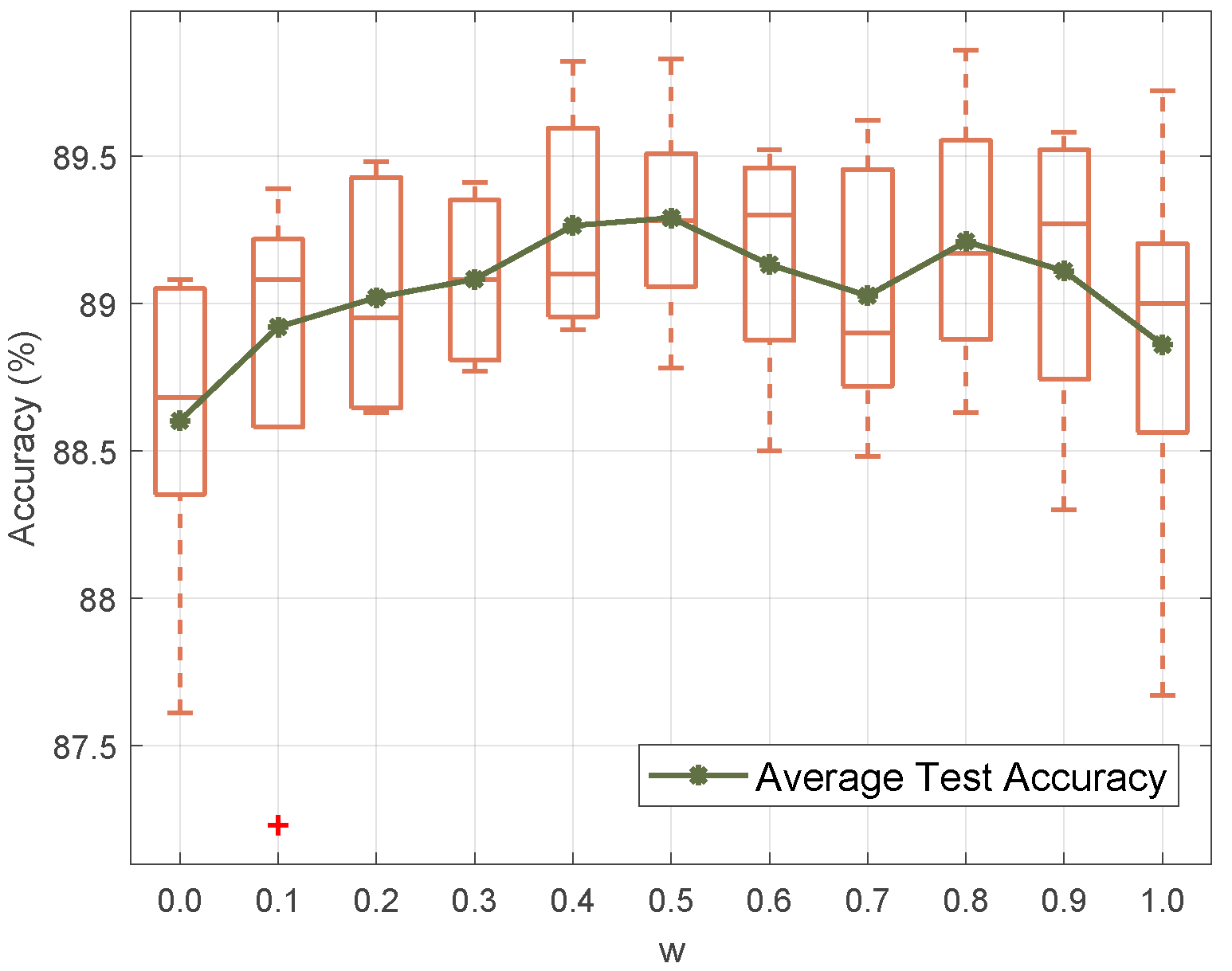
Figure 4: The average test accuracy and boxplot of five experiments about $w$ in Eq. (7).

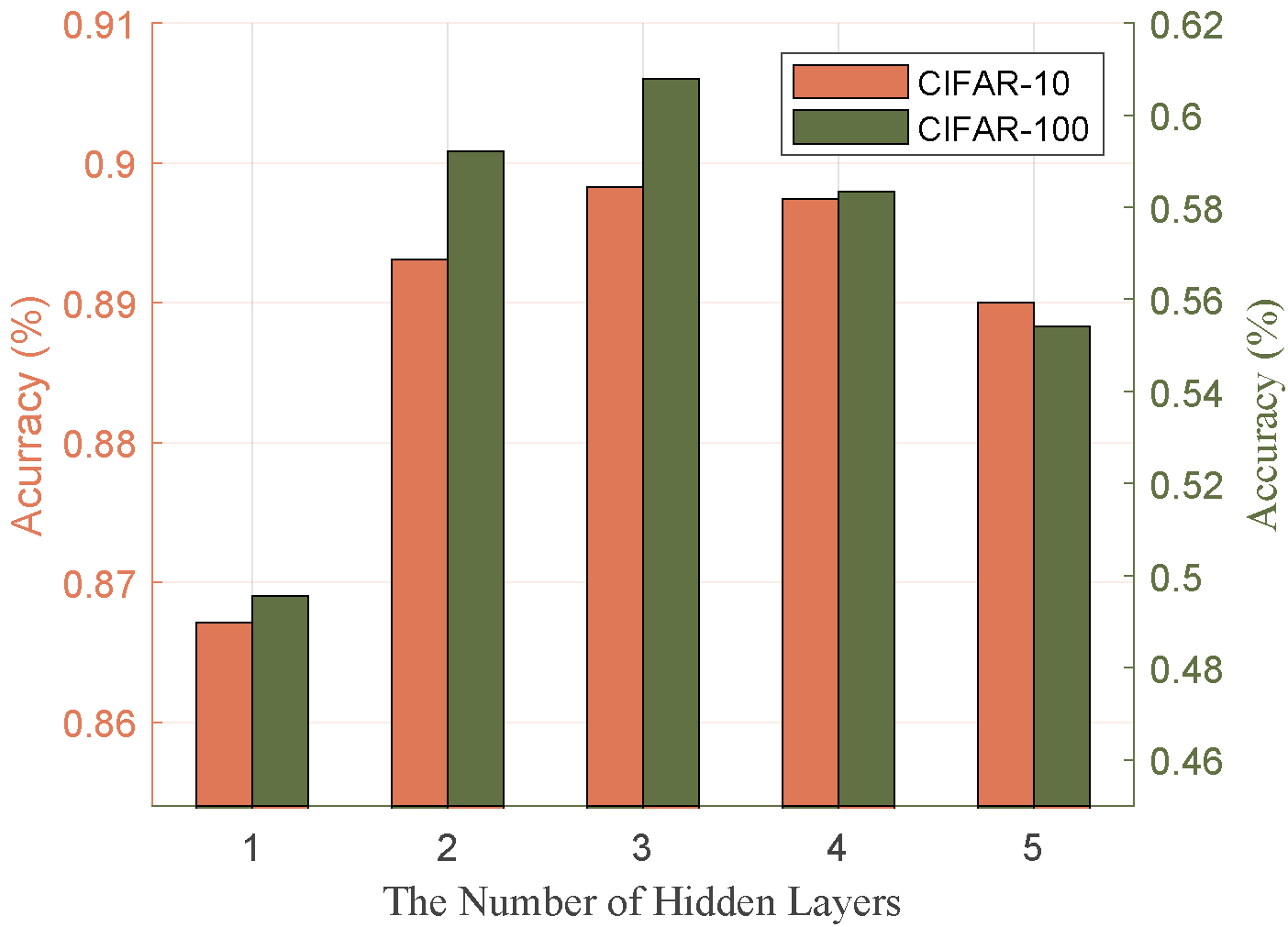
(a)

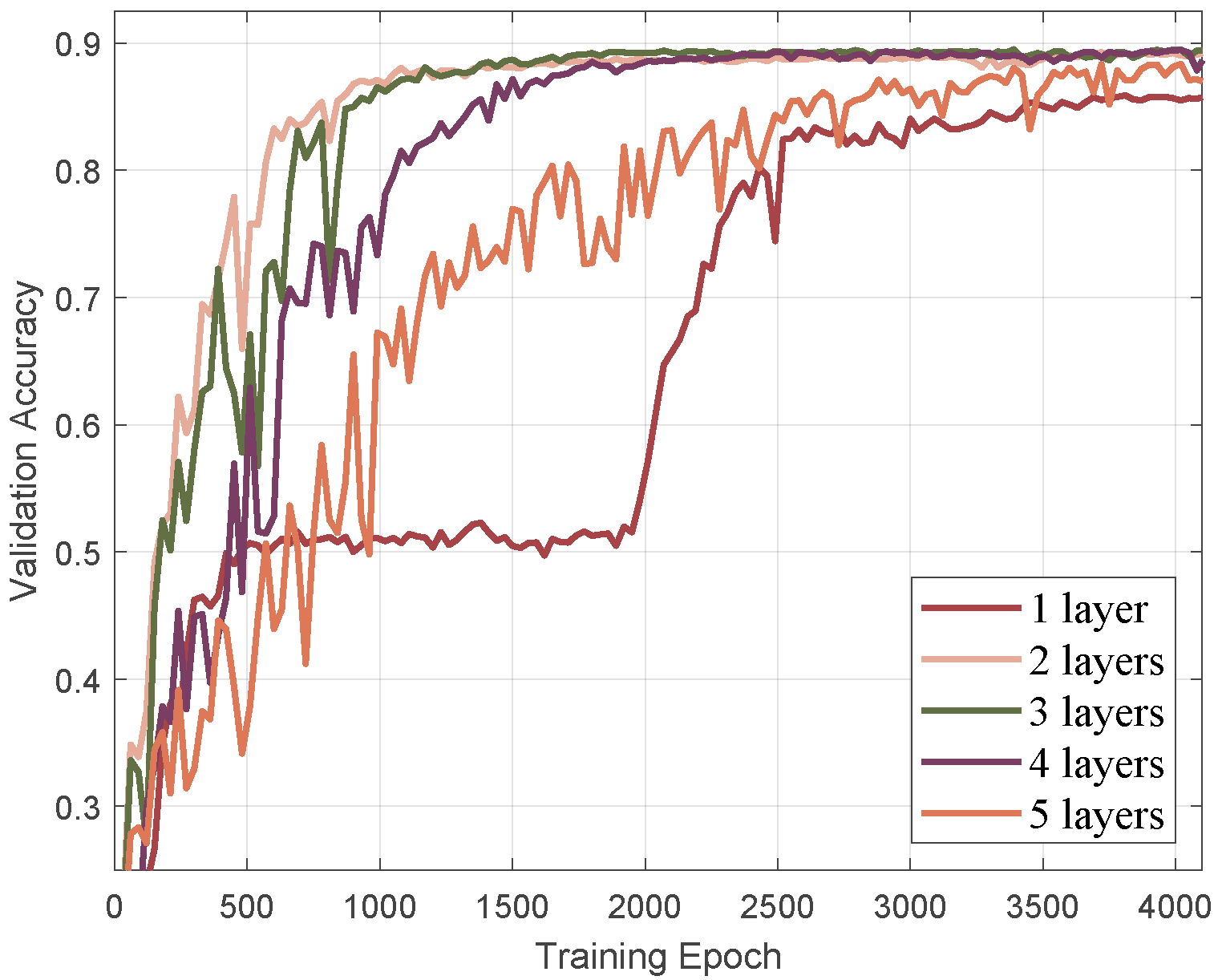
(b)

Figure 5: The impact of the hypernetwork structure. (a)-(b) represent the test accuracy on CIFAR-10/CIFAR-100 and convergence experiments on CIFAR-10, respectively.

In addition, we examine the impact of the weight parameter, denoted as $w$ in Eq. (7), with results presented in Fig. 4 across 50 clients using the CIFAR-10 dataset. The findings reveal that combining both IntraFA and InterFA leads to superior performance compared to their utilization ($w=0.0/1.0$). This observation underscores the complementarity of these two modules, with TFA capitalizing on their respective strengths for enhanced performance. We propose an empirical setting of $w=0.5$ based on our results as an optimal choice.

Lastly, we explore the impact of hypernetwork structures through experiments, as depicted in Fig. 5. Specifically, Fig. 5(a) illustrates related accuracies, while Fig. 5(b) showcases the convergence rates. Notably, a single-layer structure exhibits slower convergence, possibly due to limited representational capacity. Nevertheless, irrespective of the hypernetwork structure, our learning process consistently converges, as the theoretical proof substantiates.

6 Conclusions

This paper focuses on enhancing filters by redefining the attention mechanism to recalibrate parameters and tailor client-side model structures to specific data. We introduce FedOFA for this purpose, emphasizing filter enhancement. TFA, a key element within FedOFA, is dedicated to refining filters and exploring implicit structures. Furthermore, we propose a strategy to enforce filter orthogonality, diversifying the filter spectrum. An attention-guided pruning approach is presented for customizing local structures and optimizing communication efficiency. Theoretical evidence supports the approximation of filter-aware attention to feature-aware attention, ensuring convergence preservation. Our method distinguishes itself by enhancing performance and reducing communication costs without additional client-side expenses, making filter-aware attention promising for hypernetwork-based FL methods. However, we acknowledge the existing computational constraints that hinder modeling relationships between all filters within intricate models. This remains an open challenge and a focal point for our future work.

Supplementary Material

S1 Pseudo Code

To enhance readers’ intuitive grasp of the proposed FedOFA, we articulate the primary steps of FedOFA in Alg. 1 using pseudo-code style. For clarity and ease of comprehension, we establish key variables. The training process involves $n$ clients, denoted by $R$ and $K$, for training rounds and local training iterations. $\mathcal{L}_{orth}$ and $\mathcal{L}_{task}$ represent orthogonal regularization and task loss, respectively. The hypernetwork, client-side network, and attention module are parameterized by $\phi$, $\theta_{i}$, and $\varphi$. Additionally, $\theta^{\prime}$ signifies enhanced parameters through TFA from $\theta$. The proposed AGPS, denoted as $\operatorname{AGPS}(\cdot,p)$, generates a mask matrix $\boldsymbol{M}$ to mask $p$% of unimportant neurons, and $\odot$ signifies the element-wise dot product..

FedOFA operates on the server without imposing additional computational burdens on the client. Concurrently, our AGPS masks unimportant neurons, effectively mitigating transmission overhead. Consequently, FedOFA can be considered as a plug-and-play module to enhance performance and attain communication efficiency for hypernetwork-based methods. Notably, our approach upholds privacy by eliminating the need for local data sharing during the training process.

S2 Experiments

Our approach demonstrates notable efficacy across both CIFAR-10 and CIFAR-100 datasets. To conduct a more thorough validation of the proposed FedOFA, we extend our experiments to include the MNIST dataset [17], ensuring a comprehensive assessment of our method. Consistent with the data partition settings outlined in Section 5.1, we maintain uniformity in experimental conditions, and the results can be found in Tab. S1. It’s evident that our method consistently maintains its promising performance across diverse datasets when compared to the state-of-the-art FL methods. Furthermore, this advantage remains robust even with an increase in the number of clients.

For the input of the framework is the client embedding $\boldsymbol{v}$ with a size of 100. However, we are interested in assessing the robustness of the proposed method across varying embedding sizes. In this experiment, we treat a vanilla hypernetwork-based FL method [29] as the baseline, and the results can be found in Tab. S2. It can be noticed that the proposed FedOFA could significantly improve the performance no matter the size of $\boldsymbol{v}_{i}$, and the performance advantage is particularly pronounced when the embedding size is small.

The above experiments have thoroughly validated the superiority of the proposed FedOFA in terms of both accuracy and robustness. These performance improvements do not impose any additional client-side computational costs or increase communication overhead. Therefore, FedOFA is well-suited for computational resource limited scenarios, such as those Internet of Things environments.

1 Main Function $\triangleright$ Server Executes

2 for round $r=1,2,...,R$ do

3       Randomly select client $i\in\{1,...,n\}$

4       Generate embedding $\boldsymbol{v}_{i}$

5       $\theta_{i}\leftarrow h(\boldsymbol{v}_{i};\phi)$

6       $\theta_{i}^{\prime}\leftarrow g(\theta_{i};\varphi)$

7       $\mathcal{L}_{\operatorname{orth}}$ & Backprop $\triangleright$ Equation (8)

8       $\boldsymbol{M}_{i}\leftarrow\operatorname{AGPS}(\theta^{i},p)$

9       $\theta_{i}^{M}\leftarrow\theta_{i}^{\prime}\odot\boldsymbol{M}_{i}$

10       $\Delta\theta_{i}\leftarrow$Local Training($\theta_{i}^{M}$)

11       Update $\boldsymbol{v}_{i},\phi,\varphi$ based on $\Delta\theta_{i}$

12Local Training$(\theta_{i}^{M})$ $\triangleright$ $i$-th Client Executes

13 $\theta_{i}^{0}\leftarrow\theta_{i}^{M}$

14 for iteration $k=1,2,...,K$ do

15       Sample data $x$ and related label $\boldsymbol{y}$ from $D_{i}$

16       $y^{\prime}\leftarrow f(\boldsymbol{x},\theta)$

17       $\mathcal{L}_{\operatorname{task}}(\boldsymbol{y}^{\prime},\boldsymbol{y})$

18       Backprop & $\theta_{i}^{k}\leftarrow\theta_{i}^{k-1}-\frac{\partial\mathcal{L}_{\operatorname{task}}}{\partial\theta_{i}^{k-1}}$

19$\Delta\theta_{i}\leftarrow\theta_{i}^{k}-\theta_{i}^{0}$

return $\Delta\theta_{i}$

Algorithm 1 Main steps of FedOFA.

Table S1: Test accuracy over 50, 100, and 300 clients on MNIST.

	50	100	300
FedAvg [28]	91.69	92.50	92.59
FedProx [21]	92.34	92.86	92.86
MOON [20]	93.55	93.40	93.27
FedNova [33]	95.84	95.51	94.71
FedBN [22]	93.15	92.33	92.21
FedPer [1]	98.08	97.37	96.08
FedROD [3]	97.32	97.97	95.74
FedProto [30]	97.17	97.55	97.68
pFedHN [29]	96.79	97.20	96.14
pFedLA [27]	97.01	96.76	95.07
FedOFA	98.75	98.63	98.17

Table S2: The performance with different embedding sizes.

	50	200	300	500
baseline	87.15$\pm$1.36	88.57$\pm$1.18	88.71$\pm$0.97	88.52$\pm$0.98
FedOFA	89.84$\pm$0.21	90.49$\pm$0.29	90.57$\pm$0.13	90.06$\pm$0.14

References

- Arivazhagan et al. [2019] Manoj Ghuhan Arivazhagan, Vinay Aggarwal, Aaditya Kumar Singh, and Sunav Choudhary. Federated learning with personalization layers. arXiv preprint arXiv:1912.00818, 2019.
- Azam et al. [2021] Sheikh Shams Azam, Seyyedali Hosseinalipour, Qiang Qiu, and Christopher Brinton. Recycling model updates in federated learning: Are gradient subspaces low-rank? In Proceedings of the International Conference on Learning Representations, 2021.
- Chen and Chao [2021] Hong-You Chen and Wei-Lun Chao. On bridging generic and personalized federated learning for image classification. In International Conference on Learning Representations, 2021.
- Diao et al. [2022] Enmao Diao, Jie Ding, and Vahid Tarokh. Semifl: Semi-supervised federated learning for unlabeled clients with alternate training. In Proceedings of the Advances in Neural Information Processing Systems, 2022.
- Dinh et al. [2020] Canh T Dinh, Nguyen Tran, and Josh Nguyen. Personalized federated learning with moreau envelopes. In Proceedings of the Advances in Neural Information Processing Systems, pages 21394–21405, 2020.
- Dinh et al. [2021] Canh T Dinh, Tung T Vu, Nguyen H Tran, Minh N Dao, and Hongyu Zhang. Fedu: A unified framework for federated multi-task learning with laplacian regularization. arXiv preprint arXiv:2102.07148, 2021.
- Dosovitskiy et al. [2020] Alexey Dosovitskiy, Lucas Beyer, Alexander Kolesnikov, Dirk Weissenborn, Xiaohua Zhai, Thomas Unterthiner, Mostafa Dehghani, Matthias Minderer, Georg Heigold, Sylvain Gelly, et al. An image is worth 16x16 words: Transformers for image recognition at scale. In Proceedings of the International Conference on Learning Representations, 2020.
- Fallah et al. [2020] Alireza Fallah, Aryan Mokhtari, and Asuman Ozdaglar. Personalized federated learning with theoretical guarantees: A model-agnostic meta-learning approach. Advances in Neural Information Processing Systems, 33:3557–3568, 2020.
- Genkin et al. [2022] Alexander Genkin, David Lipshutz, Siavash Golkar, Tiberiu Tesileanu, and Dmitri Chklovskii. Biological learning of irreducible representations of commuting transformations. Advances in Neural Information Processing Systems, 35:20838–20849, 2022.
- Guo et al. [2020] Pengsheng Guo, Chen-Yu Lee, and Daniel Ulbricht. Learning to branch for multi-task learning. In Proceedings of the International Conference on Machine Learning, pages 3854–3863, 2020.
- Hou et al. [2021] Qibin Hou, Daquan Zhou, and Jiashi Feng. Coordinate attention for efficient mobile network design. In Proceedings of the IEEE/CVF Conference on Computer Vision and Pattern Recognition, pages 13713–13722, 2021.
- Hu et al. [2018] Jie Hu, Li Shen, and Gang Sun. Squeeze-and-excitation networks. In Proceedings of the IEEE Conference on Computer Vision and Pattern Recognition, pages 7132–7141, 2018.
- Huang et al. [2023] Wenke Huang, Mang Ye, Zekun Shi, He Li, and Bo Du. Rethinking federated learning with domain shift: A prototype view. In 2023 IEEE/CVF Conference on Computer Vision and Pattern Recognition (CVPR), pages 16312–16322. IEEE, 2023.
- Jang et al. [2022] Doseok Jang, Larry Yan, Lucas Spangher, Costas J Spanos, and Selvaprabu Nadarajah. Personalized federated hypernetworks for privacy preservation in multi-task reinforcement learning. arXiv preprint arXiv:2210.06820, 2022.
- Kim and Yun [2022] Taehyeon Kim and Se-Young Yun. Revisiting orthogonality regularization: a study for convolutional neural networks in image classification. IEEE Access, 10:69741–69749, 2022.
- Krizhevsky and Hinton [2009] Alex Krizhevsky and Geoffrey Hinton. Learning multiple layers of features from tiny images. 2009.
- LeCun [1998] Yann LeCun. The mnist database of handwritten digits. http://yann. lecun. com/exdb/mnist/, 1998.
- LeCun et al. [1998] Yann LeCun, Léon Bottou, Yoshua Bengio, and Patrick Haffner. Gradient-based learning applied to document recognition. Proceedings of the IEEE, 86:2278–2324, 1998.
- Li et al. [2022] Hongxia Li, Zhongyi Cai, Jingya Wang, Jiangnan Tang, Weiping Ding, Chin-Teng Lin, and Ye Shi. Fedtp: Federated learning by transformer personalization. arXiv preprint arXiv:2211.01572, 2022.
- Li et al. [2021a] Qinbin Li, Bingsheng He, and Dawn Song. Model-contrastive federated learning. In Proceedings of the IEEE/CVF Conference on Computer Vision and Pattern Recognition, pages 10713–10722, 2021a.
- Li et al. [2020] Tian Li, Anit Kumar Sahu, Manzil Zaheer, Maziar Sanjabi, Ameet Talwalkar, and Virginia Smith. Federated optimization in heterogeneous networks. In Proceedings of the Machine Learning and Systems, pages 429–450, 2020.
- Li et al. [2021b] Xiaoxiao Li, Meirui Jiang, Xiaofei Zhang, Michael Kamp, and Qi Dou. Fedbn: Federated learning on non-iid features via local batch normalization. arXiv preprint arXiv:2102.07623, 2021b.
- Liang et al. [2020] Paul Pu Liang, Terrance Liu, Liu Ziyin, Nicholas B Allen, Randy P Auerbach, David Brent, Ruslan Salakhutdinov, and Louis-Philippe Morency. Think locally, act globally: Federated learning with local and global representations. arXiv preprint arXiv:2001.01523, 2020.
- Liu et al. [2021a] Quande Liu, Cheng Chen, Jing Qin, Qi Dou, and Pheng-Ann Heng. Feddg: Federated domain generalization on medical image segmentation via episodic learning in continuous frequency space. In Proceedings of the IEEE/CVF Conference on Computer Vision and Pattern Recognition, pages 1013–1023, 2021a.
- Liu et al. [2021b] Ze Liu, Yutong Lin, Yue Cao, Han Hu, Yixuan Wei, Zheng Zhang, Stephen Lin, and Baining Guo. Swin transformer: Hierarchical vision transformer using shifted windows. In Proceedings of the IEEE/CVF International Conference on Computer Vision, pages 10012–10022, 2021b.
- Lu et al. [2022] Zexin Lu, Wenjun Xia, Yongqiang Huang, Mingzheng Hou, Hu Chen, Jiliu Zhou, Hongming Shan, and Yi Zhang. M 3 nas: Multi-scale and multi-level memory-efficient neural architecture search for low-dose ct denoising. IEEE Transactions on Medical Imaging, 42(3):850–863, 2022.
- Ma et al. [2022] Xiaosong Ma, Jie Zhang, Song Guo, and Wenchao Xu. Layer-wised model aggregation for personalized federated learning. In Proceedings of the IEEE/CVF conference on computer vision and pattern recognition, pages 10092–10101, 2022.
- McMahan et al. [2017] Brendan McMahan, Eider Moore, Daniel Ramage, and Blaise Aguera y Arcas. Communication-efficient learning of deep networks from decentralized data. In Artificial Intelligence and Statistics, pages 1273–1282, 2017.
- Shamsian et al. [2021] Aviv Shamsian, Aviv Navon, Ethan Fetaya, and Gal Chechik. Personalized federated learning using hypernetworks. In In Proceedings of the International Conference on Machine Learning, pages 9489–9502, 2021.
- Tan et al. [2022] Yue Tan, Guodong Long, Lu Liu, Tianyi Zhou, Qinghua Lu, Jing Jiang, and Chengqi Zhang. Fedproto: Federated prototype learning across heterogeneous clients. In Proceedings of the AAAI Conference on Artificial Intelligence, pages 8432–8440, 2022.
- Vaswani et al. [2017a] Ashish Vaswani, Noam Shazeer, Niki Parmar, Jakob Uszkoreit, Llion Jones, Aidan N. Gomez, Łukasz Kaiser, and Illia Polosukhin. Attention is all you need. In Proceedings of the 31st International Conference on Neural Information Processing Systems, page 6000–6010, Red Hook, NY, USA, 2017a. Curran Associates Inc.
- Vaswani et al. [2017b] Ashish Vaswani, Noam Shazeer, Niki Parmar, Jakob Uszkoreit, Llion Jones, Aidan N Gomez, Łukasz Kaiser, and Illia Polosukhin. Attention is all you need. In Proceedings of the Advances in Neural Information Processing Systems, 2017b.
- Wang et al. [2020] Jianyu Wang, Qinghua Liu, Hao Liang, Gauri Joshi, and H Vincent Poor. Tackling the objective inconsistency problem in heterogeneous federated optimization. In In Proceedings of the Advances in Neural Information Processing Systems, pages 7611–7623, 2020.
- Woo et al. [2018] Sanghyun Woo, Jongchan Park, Joon-Young Lee, and In So Kweon. Cbam: Convolutional block attention module. In Proceedings of the European Conference on Computer Vision, pages 3–19, 2018.
- Wu et al. [2022] Chuhan Wu, Fangzhao Wu, Lingjuan Lyu, Yongfeng Huang, and Xing Xie. Communication-efficient federated learning via knowledge distillation. Nature communications, 13(1):2032, 2022.
- Xie et al. [2017] Di Xie, Jiang Xiong, and Shiliang Pu. All you need is beyond a good init: Exploring better solution for training extremely deep convolutional neural networks with orthonormality and modulation. In Proceedings of the IEEE Conference on Computer Vision and Pattern Recognition, pages 6176–6185, 2017.
- Xie et al. [2021] Ruobing Xie, Zhijie Qiu, Jun Rao, Yi Liu, Bo Zhang, and Leyu Lin. Internal and contextual attention network for cold-start multi-channel matching in recommendation. In Proceedings of the International Conference on International Joint Conferences on Artificial Intelligence, pages 2732–2738, 2021.
- Yang et al. [2022] Ziyuan Yang, Wenjun Xia, Zexin Lu, Yingyu Chen, Xiaoxiao Li, and Yi Zhang. Hypernetwork-based personalized federated learning for multi-institutional ct imaging. arXiv preprint arXiv:2206.03709, 2022.