The allosteric lever: towards a principle of specific allosteric response

Abstract

Allostery, the phenomenon by which the perturbation of a molecule at one site alters its behavior at a remote functional site, enables control over biomolecular function. Allosteric modulation is a promising avenue for drug discovery and is employed in the design of mechanical metamaterials. However, a general principle of allostery, i.e. a set of quantitative and transferable “ground rules”, remained elusive. It is neither a set of structural motifs nor intrinsic motions. Focusing on elastic network models, we here show that an allosteric lever—a mode-coupling pattern induced by the perturbation—governs the directional, source-to-target, allosteric communication: a structural perturbation of an allosteric site couples the excitation of localized hard elastic modes with concerted long range soft-mode relaxation. Perturbations of non-allosteric sites instead couple hard and soft modes uniformly. The allosteric response is shown to be generally non-linear and non-reciprocal, and allows for minimal structural distortions to be efficiently transmitted to specific changes at distant sites. Allosteric levers exist in proteins and “pseudoproteins”—networks designed to display an allosteric response. Interestingly, protein sequences that constitute allosteric transmission channels are shown to be evolutionarily conserved. To illustrate how the results may be applied in drug design, we use them to successfully predict known allosteric sites in proteins.

Allosteric proteins display specific responses of functionally active sites to the binding of ligands at, typically remote, allosteric sites [1]. With the exception of dynamic, entropy driven allosteric systems [2, 3, 4, 5], the allosteric response involves conformational changes [6, 7, 8]. These have been studied experimentally [9, 10, 11, 12] (meanwhile also on the level of individual molecules [13, 14, 15, 16, 17, 18, 19]), using computational approaches [20, 21, 22, 23, 24, 25, 26, 27] (also combined with experiments [28]), as well as theoretically by means of graph theory [29, 30, 31] or distance geometry [32], and statistical structure analysis [33, 34]. Allostery is not limited to proteins; DNA [35, 36, 18, 19], RNA [37, 38], and complexes of proteins and RNA [39] display allostery as well. Allosteric control over conformations is a promising new avenue for drug discovery [40, 41] and is furthermore employed to design mechanical metamaterials with complex responses [42, 43, 44, 45, 46]. Allosteric concepts were recently extended to the control of flow in complex networks [47].

Since the pinoeering discovery of switch-like behavior in oxygen binding to haemoglobin [48], our understandind of allostery as a general action at a distance phenomenon came a long way. From the early phenomenological “population shift” [49] and “induced fit” models [50], as well as Eigen’s generalization combining both [51], which all relied heavily on static crystallographic structures of proteins, the focus gradually shifted towards understanding the microscopic, dynamic basis of the effect. Moreover, whereas initially only multimeric proteins were thought to display allostery, it was later also found in monomeric proteins [52]. Despite successful applications of these early models and their various recent generalizations and refinemenets [53, 54, 55], phenomenological models have shortcomings. In particular, the structural coupling between the allosteric source and functional sites cannot be resolved with a purely thermodynamic approach [56, 57, 58, 59].

Notwithstanding individual successes in explaining the structural determinants of allostery in well-documented systems [7, 40, 60] and in designing mechanical metamaterials [43, 44, 61, 45, 46], a general mechanism that gives rise to allostery still eludes understanding [62, 54, 55, 59]. Functional allosteric motions are specific [7], generally non-linear [63, 64, 65], and require concerted rearrangements [7]. In contrast to simply cooperative networks displaying single soft-mode responses [66], functional responses of proteins typically require coordinated motions that depend on the network structure in a complex manner [63, 45]. As a result, it is much easier to predict the response to a given perturbation [61, 64, 65, 67] than to identify the source site that upon perturbation yields a specific allosteric response. A general strategy for identifying allosteric source-target pairs that carry a desired, functional response remains elusive.

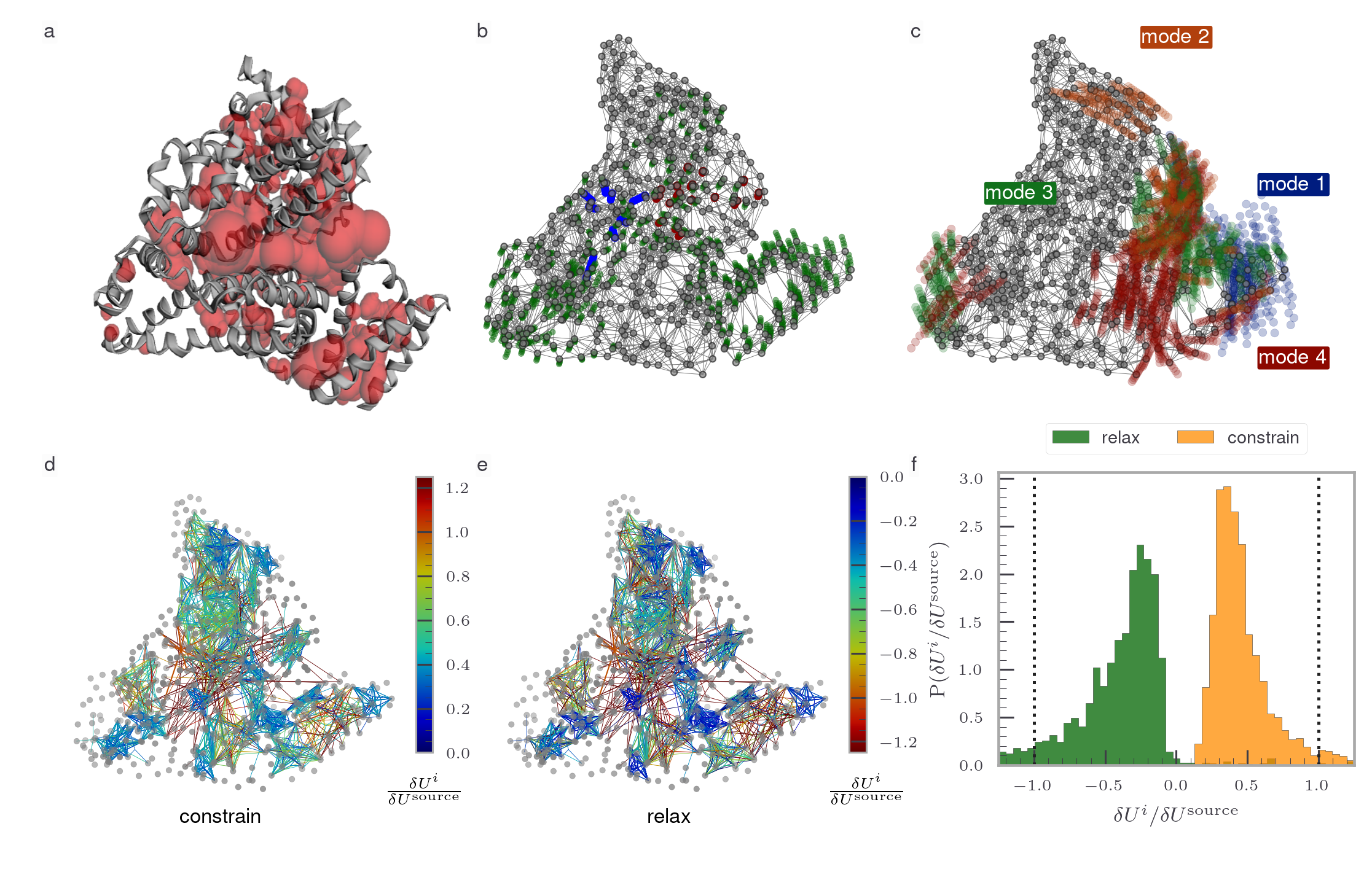
Figure 1: Mechanical perturbation of binding-pocket candidates reveals unique character of allosteric sites. (a) Cartoon representation of the Human Serum Albumin protein (HSA, PDB ID: 2bxd [68]) showing binding-pocket candidates (red) determined based on geometrical arguments [69]. Only the largest 9 of the total of 77 analyzed pockets are shown. (b) Elastic network model of the protein in a, coarse grained on a residue level; the beads are centered at carbon-$\alpha$ positions. The input perturbation at the allosteric source site and the corresponding nonlinear response are shown in blue and green, respectively; The response of beads in the biologically active pocket (i.e. “target”) is highlighted in red. The source and target site are the known binding sites of warfarin and heme, respectively. (A movie of the response trajectory is given in the SM.) (c) The four softest nonzero eigenmodes of the Hessian of the unconstrained network in (b) superimposed on the structure (only substantial motions are shown); Note the complete lack of soft-mode participation in the response of source-pocket beads. (d-f) Energy changes accompanying contractions of binding-pocket candidates during loading (d) and relaxation (e) The colors denote the energy change $\delta U^{i}$ upon contraction of the $i$th pocket (d) and during the corresponding relaxation (e) relative to that of closing the actual source binding site $\delta U^{\rm source}$. (f) Statistics over all source-pocket candidates for the constraining and relaxation steps presented as green are orange histograms, respectively. Dotted lines indicate $\delta U^{\rm source}$ of closing the true source pocket. Note that only a few pockets show substantial energy changes. Allosteric source sites seemingly enable the largest energy uptake and transmission upon mechanical perturbations.

Minimal Elastic Network Models [70] have proven invaluable for studying allostery in numerous proteins [71, 8] and for designing mechanical networks with programmed responses [43, 44, 61]. However, even here a general understanding of the transmission of an allosteric signal from a source site into a specific, functionally relevant rearrangement of the target site [7] so far was out of reach.

From a mechanical perspective it is well understood how the curvature of the potential energy surface encodes collective motions—the eigenmodes of the Hessian—of elastic networks, which was fruitfully exploited in the design of “simply cooperative” networks [43, 72]. Nevertheless, a specific rearrangement of the target site must generally involve a balanced interplay of many collective modes. Concurrently, a given input perturbation of an allosteric source site should intuitively “dissipate” the minimal amount of the perturbation energy near the source in order to allow substantial long-distance rearrangements at the target site.

The difficulty in elucidating generic allosteric mechanisms is rooted in the fact that although some allosteric responses are classifiable into intuitively understandable motions, e.g. hinge, shear, piston-like, twist, rocking or combinations of these, most proteins resist such a classification [73, 74]. This is due to the nonexistence of discrete categories of motions; proteins can choose from a continuum of different mechanisms [75]. It is therefore conceivable that a generic “physical principle of allostery”, if existent, is not a set of common motion patterns. Instead it rather seems to be a particular ligand-binding induced coupling pattern of many complex modes that enables an efficient channeled transmission of elastic perturbations in a network.

By analyzing 14 different allosteric proteins with known source-target pairs deposited in the Protein Data Bank and generating a set of 30 artificial “pseudoproteins” trained to display a specific allosteric response, we here provide evidence that fully supports the above hypothesis. We propose a conceptual shift, the allosteric lever—a structural perturbation of the allosteric source site couples hard and soft anharmonic elastic modes, which allows for an efficient, directed (i.e. non-reciprocal), and specific transmission to a distant target site. An extensive analysis of the energetics and local spectral properties of the response confirms our idea. Moreover, protein sequence patterns involved in allosteric transmission channels are found to be evolutionarily conserved. We use the allosteric-lever principle to successfully predict known allosteric sites in proteins.

The manuscript is structured as follows. In Sec. I we describe the model and its parameterization and present a new method to determine the full (i.e. beyond linear) allosteric response. In Sec. II we analyze the energetics of allosteric responses and formulate the allosteric lever hypothesis. Next, in Sec. III we establish that allosteric responses are in general non-linear and non-reciprocal. In Sec. IV we show that true (functional) allosteric responses are specific, and in Sec. V we demonstrate how already the most basic version of our findings may be utilized to predict allosteric binding sites in proteins. In Sec. VI we find that protein sequence patterns that comprise allosteric transmission channels are evolutionary conserved. We conclude with a perspective and give an outlook on future research directions that are provoked by our findings.

I Setup and mechanical response

I.1 Model and parameterization

Throughout we focus on the Elastic Network Model (ENM) used to describe the long-timescale dynamics of proteins on the coarse-grained level of amino acids [76]. The nodes of the network are beads connected by Hookean springs with stiffness $\kappa$ (see Fig. 1). Denoting the position of bead $i$ by $\mathbf{r}_{i}$, the configuration of the entire network with the super-vector $\mathbf{R}=(\mathbf{r}_{1},\ldots,\mathbf{r}_{N})^{T}$ and the equilibrium (i.e. minimum-energy) configuration by $\mathbf{R}_{\rm eq}=(\mathbf{r}_{1,{\rm eq}},\ldots,\mathbf{r}_{N,{\rm eq}})^{T}$, the distance between a pair of beads $i$ and $j$ by $r_{ij}\equiv|\mathbf{r}_{i}-\mathbf{r}_{j}|$, and the stiffness and equilibrium “rest length” of the bond connecting a pair of beads by $r_{ij}^{0}=|\mathbf{r}_{i,{\rm eq}}-\mathbf{r}_{j,{\rm eq}}|$, respectively, the potential energy of a configuration $\mathbf{R}$ is given by

$$U_{\rm EN}(\mathbf{R})=\frac{1}{2}\sum_{i>j}\kappa{\rm A}_{ij}(r_{ij}-r_{ij}^{0})^{2},$$ (1)

where ${\rm A}$ is the adjacency matrix of the underlying graph with elements ${\rm A}_{ij}=\mathbbm{1}_{r^{0}_{ij}\leq r_{c}}$ with cut-off distance $r_{c}$ and $\mathbbm{1}_{\chi}$ being the indicator function of the set $\chi$. Note that the interactions (1) are manifestly an-harmonic in $\mathbf{R}$.

The construction of ENM representations of proteins is well established and straightforward. Briefly, we retrieve the positions and atomic assignments from the Protein Data Bank (PDB) and extract the $\alpha$-carbons (i.e. the principal protein-backbone carbon). A cutoff distance $r_{c}$ is chosen as the smallest distance at which exactly 6 eigenvalues of the Hessian matrix of $U_{\rm ENM}$ are zero. $\alpha$-carbons closer than $r_{c}$ are then connected with Hookean springs, and without much loss of generality we set the spring stiffness to $\kappa=1$. The $r_{c}$ determined for various proteins all lie within $8\,\mbox{\AA}\leq r_{c}\leq 14\,\mbox{\AA}$ in agreement with existing literature [77, 78, 79] (See Table A1 for details). Notably, the results are insensitive to the choice of $r_{c}$, i.e. a small change of $r_{c}$ in the above range causes no qualitative changes [77]. We neglect effects of rigid-body motions and constraints imposed on the protein by the crystalline environment [80]. Accounting for these effects may yield more accurate specific models in terms of experimental B-factors, but is not required for our purpose as we are in pursuit of general findings. In total we analyzed 14 different allosteric proteins from the PDB for which both, the structure and allosteric binding sites are known.

In order to avoid potential unphysical configurations during the training and response of artificial “pseudoproteins”—networks we design to mimic the structure and dynamics of globular proteins—we also include the repulsive Weeks-Chandler-Andersen pair potential between beads not connected by a spring

$$U_{\rm WCA}(\mathbf{R}) = 4\epsilon\sum_{j>i}\kappa({\rm A}_{ij}-\delta_{i,j})\mathbbm{1}_{r_{ij}\leq 2^{1/6}\sigma}$$ (2)

$$\times \left[\left(\frac{\sigma}{r_{ij}}\right)^{12}-\left(\frac{\sigma}{r_{ij}}\right)^{6}+\epsilon\right],$$

where $\delta_{ij}$ denotes Kronecker’s delta. In the case of protein-derived networks the inclusion of $U_{\rm WCA}$ is not required, as no uphysical configurations occur during the response.

The determination of binding pockets in proteins is described in Appendix A. Moreover, the method to construct and train artificial pseudoproteins to exhibit an allosteric response is detailed in Appendix B. The elucidation of binding-pocket candidates in pseudoprotein networks is described in Appendix C.

I.2 Full nonlinear mechanical response

Neglecting inertial effects, which is justified by the low Reynolds number of aqueous media and the fact that internal friction in proteins is similar to that of water [81], we may determine the response of the configuration of the network to an external force due to ligand binding as the numerical solution of the overdamped Newton’s equations of motion discretized in time [61], or alternatively, by means of gradient descent upon constraining the position of the subset of source beads [64, 65, 67, 82]. However, as the latter are computationally expensive for large networks, we develop an equivalent but more efficient approach we refer to as recursive constrained quadratic optimization, a recursive piece-wise linear response problem. Notably, our approach circumvents the numerically expensive inversion of the Hessian [83].

Given a set of instantaneous coordinates $\mathbf{R}^{(0)}$ (not necessarily equilibrium ones) we aim to determine the minimum energy configuration of the network upon constraining the subset of source beads. For small deviations around $\mathbf{R}^{(0)}$, which we control by appropriately adjusting the step size in changing the constraint, we can expand the potential to second order in $\mathbf{R}^{(0)}$

$$U_{2}(\mathbf{R}|\mathbf{R}^{(0)})\!=\!\frac{1}{2}(\mathbf{R}-\mathbf{R}^{(0)})^{T}{\textsf{H}}(\mathbf{R}-\mathbf{R}^{(0)})\!+\!U(\mathbf{R}^{(0)}),$$ (3)

where H is the $3N\times 3N$ Hessian super-matrix with elements ${\textsf{H}}^{\alpha\beta}_{kl}=\partial_{\alpha_{k}}\partial_{\beta_{l}}U|_{\mathbf{R}^{(0)}}$ for beads $k$ and $l$ and $\alpha,\beta=x,y,z$, and the linear term $U(\mathbf{R}^{(0)})$ does not vanish for configurations that differ from the equilibrium configuration $\mathbf{R}^{(0)}\neq\mathbf{R}_{\rm eq}$. We set $U=U_{\rm ENM}$ for protein-derived networks and $U=U_{\rm ENM}+U_{\rm WCA}$ for pseudoproteins. We split the positions $\mathbf{R}$ into constrained source beads, which we encode in the super-vector $\mathbf{c}$, and the remaining responding beads $\mathbf{s}$, i.e.

$$\mathbf{R}\equiv\binom{\mathbf{c}}{\mathbf{s}},\quad\mathbf{R}^{(0)}\equiv\binom{\mathbf{c}^{(0)}}{\mathbf{s}^{(0)}},$$ (4)

and correspondingly also partition the instantaneous Hessian in four blocks

$${\textsf{H}}=\begin{pmatrix}{\textsf{C}}&{\textsf{B}}^{T}\\ {\textsf{B}}&{\textsf{S}}\end{pmatrix}.$$ (5)

The quadratic form (3) can now be rewritten as

$$U_{2}(\mathbf{R}|\mathbf{R}^{(0)})\!=\!\frac{1}{2}\mathbf{s}^{T}\,{\textsf{S}}\,\mathbf{s}+([\mathbf{c}-\mathbf{c}^{(0)}]^{T}{\textsf{B}}-\mathbf{s}^{(0)}{\textsf{S}})\mathbf{s}+{\rm const},$$ (6)

where the constant term is irrelevant for the omptimization problem. For a given constraint $\mathbf{c}$ the response is obtained as the solution of $\nabla_{\mathbf{s}}U_{2}=\mathbf{0}$, which reads

$$\mathbf{s}=\mathbf{s}^{(0)}-{\textsf{S}}^{-1}{\textsf{B}}^{T}(\mathbf{c}-\mathbf{c}^{(0)}),$$ (7)

and involves only the numerical inversion of the smaller block S. The splitting of the matrix (5) is equivalent to that used in [71], and the implicit formulation of the response induced by deforming a binding pocket (7) was derived in [84]. However, to determine the full nonlinear response of the free beads to the perturbation of the source beads, we here apply the above method recursively as follows.

We discretize the source perturbation into small steps yielding a “constraint trajectory”, $\mathbf{c}(k),\,k=0,\ldots,N_{\rm step}$ and an instantaneous Hessian at each $\mathbf{R}^{(0)}=\mathbf{R}(k-1)$ in Eq. (3), ${\textsf{H}}_{k-1}\equiv{\textsf{H}}(\mathbf{R}(k-1))$, and we solve for the free beads $\mathbf{s}(k)$, yielding the full response trajectory $\mathbf{R}(k)$ via Eq. (4) with $\mathbf{R}(0)=\mathbf{R}_{\rm eq}$. The step size $\mathbf{c}(k+1)-\mathbf{c}(k)$ is controlled such that $U_{2}(\mathbf{R}(k+1))=U(\mathbf{R}(k+1))$ within numerical precision for all $k$. The instantaneous Hessian is determined from the instantaneous coordinates $\mathbf{R}(k-1)$ using the original rest lengths of the springs $\{r^{0}_{ij}\}$. The full nonlinear response trajectory thus reads

$$\mathbf{R}(k)=\inf_{\mathbf{R}}\,[\mathbf{R}^{T}{\textsf{H}}_{k-1}\mathbf{R}\,\big{|}\,\mathbf{R}_{i\in S}=\mathbf{c}(k)],$$ (8)

and is obtained by recursively solving Eq. (7). We neglect the possibility of multiple solution trajectories $\mathbf{R}(k)$ for a given input $\mathbf{c}(k)$; these are indeed unlikely but potentially possible in highly symmetric networks. Conversely, the linear response corresponds to the single-step solution of Eq. (7) imposing the full constraing $\mathbf{c}(N_{\rm step})$ , i.e. $\mathbf{s}=\mathbf{s}^{(0)}-{\textsf{S}}_{0}^{-1}{\textsf{B}}_{0}^{T}(\mathbf{c}(N_{\rm step})-\mathbf{c}^{(0)})$. The full response to closing an allosteric pocket in the HSA protein is illustrated in Fig. 1b (green trajectory) with source (blue beads) and target (red beads) sites which are the known binding sites of warfarin and heme, respectively.

II Response to local perturbation and allosteric lever

As the initial step we construct ENMs (proteins and pseudoproteins), determine the binding-pocket candidates, and evaluate the full response to closing these individually, as detailed in Sec. I. Moreover, for each configuration $\mathbf{R}(k)$ during the response (see Eq. (8)) we determine the spectrum of the instantaneous Hessian ${\textsf{H}}_{k}$

$${\textsf{H}}_{k}\mathbf{v}_{l}(k)=\omega_{l}(k)\mathbf{v}_{l}(k),\quad k=0,\ldots,N_{\rm step}\,,$$ (9)

where $\mathbf{v}_{l}(k)$ is the $l$-th (column) eigenvector (for an illustration see the first 4 nonzero eigenmodes of the HSA protein in Fig. 1c) and $\omega_{l}(k)$ the corresponding eigenvalue. Eigenmodes with small $\omega_{k}$ are “soft” because their excitation requires only little energy. Conversely, modes with large $\omega_{k}$ are said to be “stiff” as they entail a large local curvature of $U$ and thus display greater resistance against perturbations. As they are irrelevant, rigid-body motions (i.e. zero modes) are systematically removed in the analysis as described in Appendix D.

In contrast to “simply cooperative” elastic networks displaying responses which can be explained with a single “dominant” soft-mode of the unperturbed state [66], functional responses of proteins typically involve coordinated motions, depending on the structure in a complex manner [63, 45]. As a result, the allosteric response generally cannot be rationalized in terms of soft modes alone. To visualize this, we compare in Fig. 1 the full response of the HSA protein to closing the allosteric binding pocket for the drug warfarin (panel b, green trajectory) with the 4 softest modes of the unperturbed network (panel c). Note that (i) the softest mode does not participate at all in the response of the target site (red beads in Fig. 1b) and, more strikingly, none of the four softest modes participates in the closing of the source pocket (blue beads in Fig. 1b). That is, the perturbation and response are orthogonal to the four softest eigenmodes of the resting network.

Based on (i) the fact that allostery is not a set of common motion patterns [73, 74], (ii) is a property of all proteins that is merely amplified in “allosterically active” ones [7], (iii) functional allosteric responses require concerted long-range motions involving multiple modes [63, 45], and (iv) an optimal transmission of a structural perturbation from the source to the target should “dissipate” the minimal amount of energy near the source pocket, we formulate the following central

Hypothesis (Allosteric lever).

Allostery is an evolutionarily optimized coupling pattern between anharmonic modes induced by ligand binding; the perturbation of the source pocket preferentially loads stiff modes and relaxes along a fine-tuned mixture of softer modes that specificially rearrange the target pocket. Accordingly

1. both, loading and relaxation energy are extremized

2. the response is non-reciprocal and non-linear

3. the true source pocket effects a specific response

4. allosteric transmission channels are conserved through evolution

The first point can be tested in a natural and straightforward manner. According to Eq. (8) we split the response into two steps (in a “Trotter” fashion [86]): the constraining step $\delta\mathbf{c}_{k}\equiv\mathbf{c}(k)-\mathbf{c}(k-1)$ and the relaxation step $\delta\mathbf{s}_{k}\equiv\mathbf{s}(k)-\mathbf{s}(k-1)$ (see Eq. (4)). Accordingly, the energy take-up during loading is given by (see Eqs. (4-7))

$$\delta U(\delta\mathbf{c}_{k})=\frac{1}{2}\delta\mathbf{c}^{T}_{k}{\textsf{C}}_{k}\delta\mathbf{c}_{k},$$ (10)

while the energy release during relaxation reads

$$\delta U(\delta\mathbf{s}_{k}) = \frac{1}{2}\delta\mathbf{R}^{T}_{k}{\textsf{H}}_{k}\delta\mathbf{R}_{k}-\frac{1}{2}\delta\mathbf{c}^{T}_{k}{\textsf{C}}_{k}\delta\mathbf{c}_{k}$$ (11)

$$= \frac{1}{2}\delta\mathbf{s}^{T}_{k}{\textsf{S}}_{k}\delta\mathbf{s}_{k}+\delta\mathbf{s}^{T}_{k}{\textsf{B}}_{k}\delta\mathbf{c}_{k}$$

$$= -\frac{1}{2}\delta\mathbf{c}_{k}^{T}{\textsf{B}}_{k}{\textsf{S}}_{k}^{-1}{\textsf{B}}_{k}^{T}\delta\mathbf{s}_{k},$$

where in the last line we used Eq. (7). In the analysis we consider all steps of the response and perturb the pocket to a fixed percentage of its initial radius of gyration. To rule out trivial effects caused by different pocket sizes, we divide the energy by the number of beads in the source-pocket candidate. Moreover, to allow for a comparison of different proteins and pseudoproteins we consider energy changes relative to that of the true source pocket, i.e. $\delta U^{i}/\delta U^{\rm source}$. The energy uptake and relaxation of the true source are thus $\pm 1$, respectively.

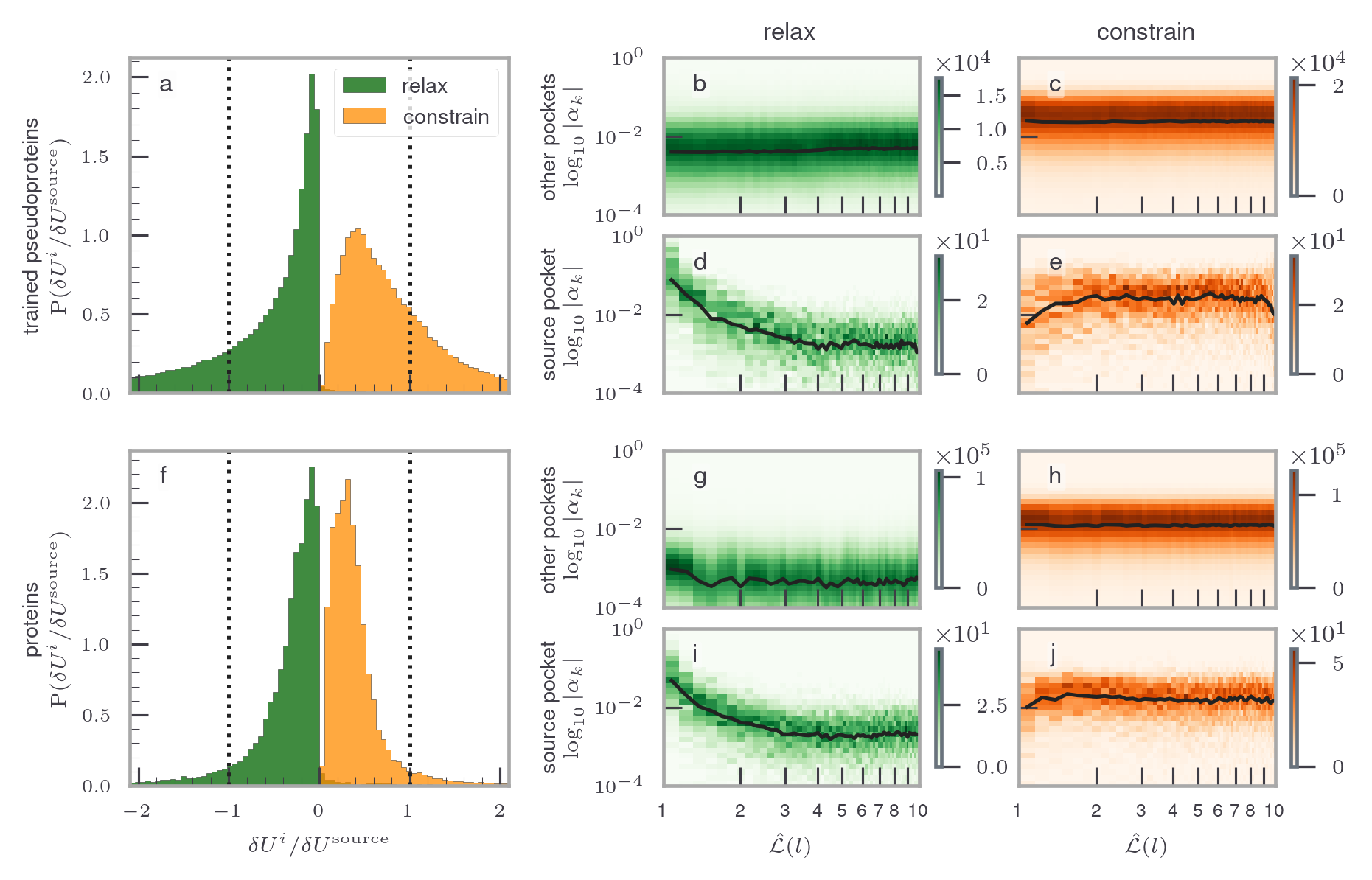
Figure 2: Energetics of two-step response unveils the allosteric lever. Statistics of $\delta U^{i}/\delta U^{s}$ for all source-pocket candidates during perturbation (orange) and relaxation (green) for pseudoproteins (a) and proteins (f); Energy changes $\delta U$ are normalized per-bead to allow for a comparison of networks and proteins with different sizes. The results of the true source pocket are highlighted with dashed lines at $\pm 1$. Alternatively we compare responses to perturbing the pocket $i$ during loading $\delta\mathbf{C}^{i}$ and relaxation $\delta\mathbf{S}^{i}$ in terms of their projections $\alpha_{k}$ onto nonzero eigenmodes of the corresponding Hessian matrix, $\mathbf{v}_{k}$ (see Eq. (12)) for pseudoproteins (b-e) and proteins (g-j) for true source pockets (bottom) and other binding-pocket candidates (top); note the logarithmic scale. To allow for a consistent comparison of structures with different sizes, the eigenmode indices $k$ are spread evenly between 1 and 10; the complete mapping onto the normalized eigenmode index is $\hat{\mathcal{K}}(k)$ (see Eq. (13)). Both pseudoproteins and proteins show uniform projections over the mode indices for non-allosteric pockets. In the case of true source pockets the perturbation does not couple to soft modes, whereas the response in fact predominantly couples to these, which we refer to as the allosteric lever. There is no qualitative difference between pseudoproteins and proteins.

This analysis of the energetics of the uptake and relaxation is illustrated for the HSA protein in Fig. 1d-f, depicting $\delta U^{i}/\delta U^{\rm source}$ projected on the particular source-pocket candidate for the uptake (d) and release (f), while the histogram over all source-pocket candidates is shown in Fig. 1e. Only a few pockets show significant energy changes, and the response of the true source pocket falls among the largest energy uptake and release, respectively. Note, however, that we find pockets producing even larger energy changes, which, however, do not necessarily correlate with a large change at the target pocket; we explain these below.

To verify that the results for the HSA protein are in fact representative, we evaluate in Fig. 2 the statistics over all pseudoproteins and all proteins. We find that the “fat tails” in the relaxation step are more pronounced than in the loading step, and that both the energy uptake and relaxation of the true source pockets in real proteins is better optimized than in pseudoproteins (compare panels a and f in Fig. 2). Here as well, we find that some source-pocket candidates display even larger energy changes that concurrently do not necessarily correlate with a large response of the target pocket. To exclude potential artifacts of sampling only subsets of the very large binding pockets instead of the full pocket, we also analyze the energetics of the response of full pockets (see Fig. A3 in Appendix A for details), where we find no qualitative difference.

The outliers with large $|\delta U^{i}/\delta U^{\rm source}|$ that are not true source pockets show that the relative energy change $\delta U^{i}/\delta U^{\rm source}$ alone is not a sufficient criterion. We show below that this is because the observable $\delta U^{i}/\delta U^{\rm source}$ does not necessarily account for the magnitude and specificity of the response of the target pocket. In fact, we show below (see Fig. 5g-j) by conditioning on the magnitude or specificity the response of the target, $\delta U^{i}/\delta U^{\rm source}$ may in fact be used to predict allosteric source sites based on purely physical arguments (neglecting all chemical details) with a quite remarkable accuracy.

To test if the observed energy changes reflect the loading of hard modes and relaxation along softer modes upon perturbing the true source pocket (in line with our hypothesis), we determine the projection of the normalized loading of source pocket $i$ for each step $k$ of the response, $\hat{\mathbf{c}}_{k}^{i}=\mathbf{c}^{i}(k)/|\mathbf{c}^{i}(k)|$ and the corresponding relaxation step $\hat{\mathbf{s}}^{i}_{k}=\mathbf{s}^{i}(k)/|\mathbf{s}^{i}(k)|$ (both augmented to the full dimensionality $\mathbbm{R}^{3N}$ with zeroes) onto the respective eigenvectors

$$\alpha_{l}(k)=\hat{\mathbf{x}}^{T}\mathbf{v}_{l}(k),\quad\hat{\mathbf{x}}=\hat{\mathbf{c}}_{k}^{i},\hat{\mathbf{s}}^{i}_{k}\,.$$ (12)

To allow for a comparison of networks and proteins with different sizes (and thus different number of eigenmodes) we divide by dimensionality $3N$ and spread the eigenmode index $l$ for each network on a logarithmic scale, yielding the normalized eigenmode index defined as

$$\hat{\mathcal{L}}(l)\equiv\log_{10}\left[\frac{9(l-6)}{3N}+1\right],\quad l=6,\ldots,3N.$$ (13)

We inspect histograms of $|\alpha_{l}|$ binned as a function of $\hat{\mathcal{L}}(l)$ for each incremental step of the response for all pseudoproteins (Fig. 2b-e) and proteins (Fig. 2g-j). We find that in comparison to “false” pockets, the perturbation of true source pockets evidently avoids coupling to soft modes (compare Fig. 2c and Fig. 2e for pseudoproteins and Fig. 2h and Fig. 2j for proteins). Even more prominently, the concurrent relaxation upon loading true source pockets predominantly involves soft modes, whereas in the case of “false” pockets it involves all modes equally (compare Fig. 2b and Fig. 2d for pseudoproteins and Fig. 2g and Fig. 2i for proteins). This is in line with our hypothesis and confirms point 1.

III Allosteric responses are non-linear and non-reciprocal

We now show that, and explain why, the allosteric response to perturbing the true source pocket is typically both, non-linear and non-reciprocal. Already upon visual comparison of the full and linear responses (see e.g. Fig. 3a) we find that they typically significantly diverge. To make the comparison quantitative, we inspect the radii of gyration of the source $r^{2}_{\rm gyr}(S)$ and target $r^{2}_{\rm gyr}(T)$ pocket defined in Eq. (A1) during the response (green line in Fig. 3b) and compare them with the linear-response approximation (orange line in Fig. 3b). Except for very small perturbation of the source, the full and linear response disagree substantially.

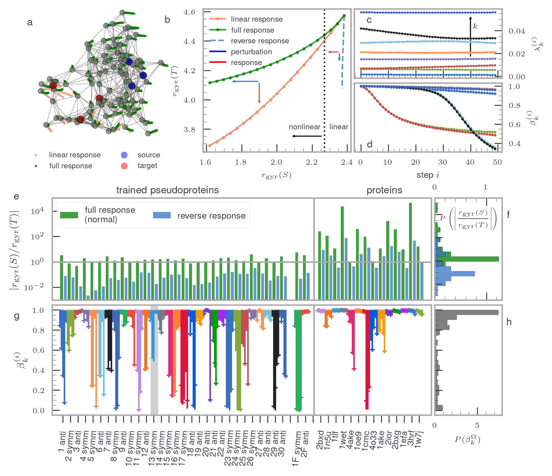
Figure 3: Allosteric response is non-reciprocal and non-linear. (a) Comparison of response trajectories of an example pseudoproteins determined by recursive constrained optimization (i.e. the “full response”; green) and by a single-step linear response (orange) for the same input. The source (blue) and target (red) pockets are highlighted for the initial configuration. (b) Corresponding radii of gyration of the input (i.e. source) $r_{\rm gyr}(S)$ and target $r_{\rm gyr}(T)$ as quantifiers of the response (in the same colors as in (a)) and the radius of gyration of the full reverse response (dashed blue line). The arrows indicate the direction of the input (blue arrow) and output (red arrow) for the normal and reverse responses, respectively. (c) Changes of the the first $8$ eigenvalues of the “instantaneous Hessian” during the response and (d) the scalar product of the corresponding eigenvectors of the “instantaneous Hessian” during the response with their initial directions, $\beta_{k}^{(i)}$ (see Eq. (14)). (e-h) Statistics of the results in (a-d) taken over all trained pseudoproteins and proteins: (e) Ratios of the input vs. output for the “forward” and reverse response providing clear evidence of non-reciprocity, histogrammed in (f) (note the two clearly distinct peaks). (g) The rotation (i.e. $\beta^{(i)}_{k}$) of the first $5$ eigenvectors for all trained pseudoproteins (including two structures designed in [61]) and the 14 analyzed proteins (the gray shaded area indicates the pseudoprotein shown in a-c). Note that in many cases the initial orientation turns perpendicular during the response, whereas for others (those displaying a linear response) it remains constant throughout the response. (h) Corresponding histogram revealing a broad range of reorientation magnitudes during the response, underscoring the limited (approximate) validity of linear response theory only for a subset of proteins.

Moreover, we compare the “forward” response to perturbing the source pocket to that of perturbing the target pocket exactly in the same manner it changes during the “forward” response. We find that the response is strongly non-reciprocal, in line with the allosteric-lever hypothesis, and is an immediate consequence of the fact that multiple eigenmodes are involved. The non-reciprocity follows directly from Eq. (7) which involves fundamentally different response matrices ${\textsf{S}}^{-1}{\textsf{B}}^{T}$ during the forward and inverse response and shows non-reciprocity also in the linear-response approximation (see also Fig. 3b). That is, non-reciprocity and non-linearity of the response are not inter-dependent.

Intuitively, imposing the constraint on the source beads and allowing the free beads to relax, we confine the latter minimization to some hypersurface. Conversely, constraining the target beads to follow precisely their former response, the hypersurface to which the free beads are confined during the reverse response is obviously different, and thus so will be the minimum-energy path. Therefore, the “forward” and reverse trajectories of the respective free beads will generally not be the same. Note that there is conclusive recent evidence for a one-way allosteric communication obtained by atomisctic Molecular Dynamics simulations [23]. For experimental evidence of a bi-directional, but not symmetric, allosteric control via photoswitching see [12]. However, the situation is different when the response goes along a single soft mode [66], since here the motion is effectively one-dimensional, such that the free beads during relaxation are confined to the same line and the response is thus manifestly reciprocal.

Hints about the origin of the non-linearity of the response in turn come from the observation of avoided crossings in the behavior of the eigenvalues of the instantaneous Hessian matrix ${\textsf{H}}_{k}$ during the full response (see Fig. 3c) and substantial rotations of the corresponding eigenvectors quantified via the projection of the instantaneous eigenvectors $\mathbf{v}_{l}(k)$ at step $k$ of the response onto those of the resting Hessian $\mathbf{v}_{l}(0)$ (see Eq. (9)), i.e.

$$\beta^{(k)}_{l}\equiv\mathbf{v}_{l}(0)^{T}\mathbf{v}_{l}(k),\quad k=0,\ldots,N_{\rm step},$$ (14)

which show large distortions of the eigendirections of normal modes during the response (see Fig. 3d). This rationalizes the failure of linear response theory but does not yet explain its origin.

Before explaining this deeper, we first check if the non-linearity and non-reciprocity of the allosteric response are a typical observation in both, pseudoproteins and proteins. Indeed, a comparison of the magnitude of the relative change at the source versus target pocket $|r^{2}_{\rm gyr}(S)/r^{2}_{\rm gyr}(S)|$ (see Fig. 3e) clearly confirms that the “forward” and reversed responses are almost always asymmetric, which is quantitatively shown in the frequency histograms of $|r^{2}_{\rm gyr}(S)/r^{2}_{\rm gyr}(T)|$ in Fig. 3f.

Similarly, the projection of the instantaneous onto the resting eigenvectors encoded in $\beta^{(k)}_{l}$ typically significantly differs from 1, indicating the failure of linear response (see Fig. 3g), which is quantified in frequency histograms of $\beta^{(k)}_{l}$ depicted in Fig. 3h. Taken together, this strengthens the evidence supporting the allosteric-lever hypothesis and in particular it confirms point 2.

III.1 Avoided eigenvalue crossings and origin of non-linear response

In Fig. 3c we observed avoided crossings of the eigenvalues of the instantaneous Hessian $\omega_{l}(k)$ (see Eq. (9)) as a result of perturbing the source pocket. We now analyze these systematically. We first determine mid-point tangents $T_{l}(k)$ for all points $k$ along the eigenvalue curves, excluding the first and last point of each curve:

$$T_{l}(k)=\frac{1}{2}[\omega_{l}(k+1)-\omega_{l}(k-1)],\,k=2,\ldots,N_{\rm step}-1,$$ (15)

and determine the points where nearest-neighbor tangents (i.e. $l$ and $l+1$) would intersect. An avoided crossing between a given pair $l$ and $l+1$ occurs when the intersection point first diverges towards $+\infty$ as a function of $k$ and subsequently re-enters from $-\infty$ (see Fig. A7 in Appendix F). Within the interval of the “discontinuity” of the intersection point, the actual location of an intersection is determined on the basis of a sign-change of $\omega_{l+1}(k)-\omega_{l}(k)$. Only instances where the crossing occurs first from above ($+\to-$) and then from below ($-\to+$) are considered. Examples of avoided eigenvalue crossings determined this way for for an artificial pseudoprotein and the HSA protein (PDB ID 2bxg [68]) are shown in Fig. 4a and Fig. 4b, respectively.

We quantify the degree of non-linearity of the response in terms of the norm of the difference between the final configuration of the full response $\mathbf{R}_{\rm fin}=\mathbf{R}(N_{\rm step})$ and the linear response approximation $\mathbf{R}^{\rm lin}_{\rm fin}$, $L_{2}(\rm full-lin)\equiv|\mathbf{R}_{\rm fin}-\mathbf{R}^{\rm lin}_{\rm fin}|$ normalized by the norm of the full response $L_{2}(\rm full-init)\equiv|\mathbf{R}(N_{\rm step})-\mathbf{R}_{0}|$. We observe a strong correlation between the degree of non-linearity and the number of avoided crossings $N_{\rm av\leavevmode\nobreak\ cross}$ relative to the number of eigenvectors $N_{\rm eigvecs}$ (see Fig. 4c). This is not surprising; avoided crossings are known to occur when vibrations (in classical as well as quantum systems [87, 88, 89]) become strongly coupled by an external perturbation.

In simple terms, it is known that there exist two fundamentally different regimes in the classical mechanics of coupled oscillators, regular (or quasiperiodic) and irregular (or chaotic/ergodic). The regular regime is similar to the motion of uncoupled oscillators, i.e. trajectories are confined to only a limited number of the energetically allowed disjoint regions (effectively the set of non-communicating trajectories of a set of uncoupled oscillators) [87, 88, 89, 90]. Conversely, in the irregular regime trajectories occupy all (or almost all) energetically allowed regions [87, 88, 89, 90]. The transition from (predominantly) regular to (predominantly) irregular motion occurs once enough energy is injected to the system or when the coupling between oscillators becomes strong enough, and is accompanied by avoided crossings in linearized spectra signaling an-harmonic resonances [87, 90]. These produce extensive changes in the eigenmodes and in the energy distribution among participating oscillators [89, 90].

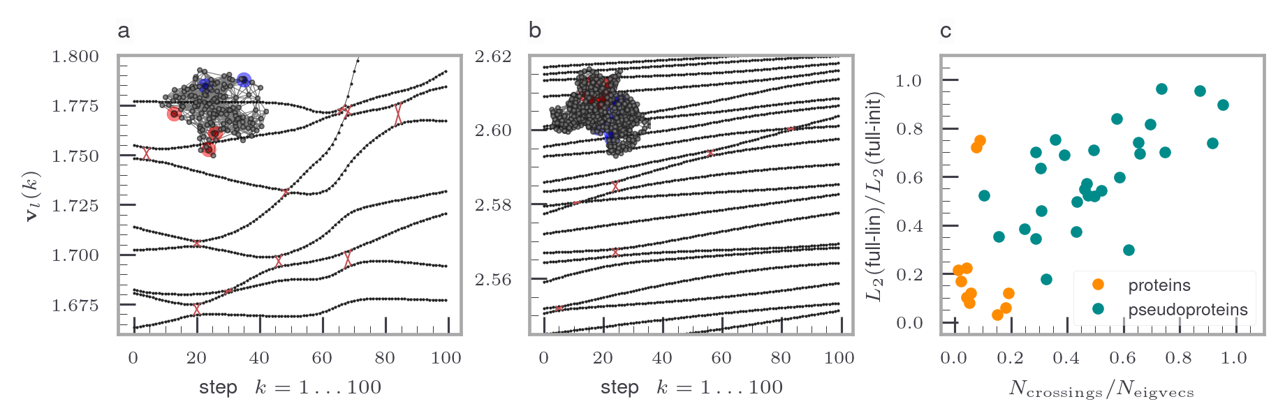
Figure 4: Nonlinear response and avoided crossings. (a-b) Eigenvalues $\mathbf{v}_{l}(k)$ of the instantaneous Hessian at the $k$-th step of the response of (a) a self-trained pseudoprotein and (b) HSA protein (PDB ID: 2bxg [68]); red crosses indicate the estimated position of avoided crossings and insets 3D representations of the respective network. (c) Scatter plot depicting a clear correlation between the number of avoided crossings (normalized by the total number of eigenvectors), $N_{\rm cross}/N_{\rm eigvecs}$, and the nonlinearity of the response quantified as the Euclidean norm of the difference between final positions of the linear and nonlinear responses divided by the Euclidean norm of the difference between nonlinear response and initial (resting) configuration; orange dots represent protein-derived networks and green ones self-trained pseudoproteins.

Applied to our allostery setting, a small perturbation of the source pocket (i.e. within the “regular” regime) only excites/deforms individual eigenmodes of the resting network, but does not couple distinct eigenmodes. In this regime the response is manifestly linear (see small-perturbation regime in Fig. 3a-b) and thus the “allosteric lever” does not yet properly unfold as there is only a very weak or even no mode coupling. Conversely, as the perturbation of the source pocket becomes stronger, modes begin to couple substantially, which is manifested in avoided crossings. Notably, it couples many modes (see Fig. 4a-b) and thus allows to transmit energy from the hard modes excited at the source pocket to soft modes in the rest of the network and in particular to the target pocket as observed in Fig. 2. This gives rise to a non-linear response and is also the mechanism of the hypothesized “allosteric lever”.

IV Specificity of allosteric responses

As announced in Sec. II, the energy changes during loading $\delta U(\delta\mathbf{c})$ and $\delta U(\delta\mathbf{s})$ in Eqs. (10-11) alone do not completely capture the essence of the allosteric-lever hypothesis, as they do not necessarily account for the magnitude and specificity of the response induced in the target pocket. Note, moreover, that a precise, specific rearrangement of the active target site is believed to be required [7]. We will show that by comparing $\delta U(\delta\mathbf{c})$ and $\delta U(\delta\mathbf{s})$ for source-pocket candidates conditioned on the magnitude and specificity of the target response, we can in fact characterize and predict allosteric source sites in proteins remarkably accurately.

Let $\mathbf{T}^{0}\in\mathbbm{R}^{3N_{T}}$ denote the initial configuration of the target pocket comprised of $N_{T}$ beads, and $\mathbf{T}_{i}^{\rm fin}\in\mathbbm{R}^{3N_{T}}$ and $\mathbf{T}_{*}^{\rm fin}\in\mathbbm{R}^{3N_{T}}$ the final response of the target upon perturbing the $i$-th surface pocket and the true/optimal source pocket, respectively. In drug design applications $\mathbf{T}_{*}^{\rm fin}\in\mathbbm{R}^{3N_{T}}$ would be the desired response. Note that only the response at the target site matters, the response of the rest of the network is irrelevant for drug design applications. We therefore apply an optimal roto-translation [91] to best overlay the respective target configurations. We introduce the relative magnitude of the response to closing the $i$-th source-pocket candidate as

$$\Delta_{i}\equiv\frac{|\mathbf{T}_{i}^{\rm fin}-\mathbf{T}^{0}|}{|\mathbf{T}_{*}^{\rm fin}-\mathbf{T}^{0}|},$$ (16)

and the relative distance from the desired response as

$$D_{i}\equiv\frac{|\mathbf{T}_{i}^{\rm fin}-\mathbf{T}_{*}^{\rm fin}|}{|\mathbf{T}_{*}^{\rm fin}-\mathbf{T}^{0}|}.$$ (17)

For convenience we introduce the response specificity as

$$0\leq\mu_{i}\equiv(1+D_{i})^{-1}\leq 1$$ (18)

such that the desired/optimal response has relative magnitude and specificity one, $\Delta_{*}=\mu_{*}=1$. Triangle inequalities between the norms in Eqs. (16-17) (see for details) confine all responses to the domain

$$\frac{1}{2+\Delta_{i}}\leq\mu_{i}\leq\frac{\theta(1-\Delta_{i})}{2-\Delta_{i}}+\frac{\theta(\Delta_{i}-1)}{\Delta_{i}},$$ (19)

where $\theta(x)$ is the Heaviside function being $1$ when $x>0$, $1/2$ when $x=0$, and $0$ otherwise.

We assume now that the target site is known. The aim is to allosterically control and rearrange this target in a specific, desired manner in order to modulate the binding of ligands. The allosteric source pocket is in turn unknown and to be determined. Note that enforcing the desired response at the target site and simply observing the rest of the network to deduce the allosteric site is not possible, because the response was found to be non-reciprocal, see Sec. III. Therefore, whereas this might work in rare reciprocal systems (see e.g. [93, 94]), discovering allosteric sites by assuming a reciprocal bidirectional coupling will generally fail.

We scan the response of all possible pocket pairs and triplets, for proteins also larger pockets (see Eq. (8)). Nearest neighbors of the target pocket are omitted from the scan. The computing time for all 14 proteins and 33 pseudoproteins is only a few hours on a medium-sized compute cluster. The exact number of scanned pocket candidates is given in Tables A1 and A2. The joint probability density of magnitude and specificity, $p(\Delta,\mu)$, and both marginals, $p(\Delta)$ and $p(\mu)$, over all pseudoproteins and proteins are shown in Fig. 5.

Figure 5: Optimal source pockets efficiently transmit energy and yield large and specific allosteric responses. Joint frequency histograms of magnitude $\Delta$ and specificity $\mu$, $p(\Delta,\mu)$ (defined in Eqs. (16) and (18), respectively) and their marginals, $p(\Delta)$ and $p(\mu)$, for adjacent pairs of beads on the surface of pseudoproteins (a) and proteins (b). The histograms are evaluated for $\Delta_{i}$ and $\mu_{i}$ for all pairs $i$ of surface beads normalized with respect to the given network, and the statistics is determined over all networks. The black lines denote the bounds imposed by the three triangle inequalities between the norms in Eqs. (16-17). Green arrows point to the ideal response at $(1,1)$. The latter may not necessarily be reached in practical applications (e.g. in drug design); in this case source candidates nearest to the optimum are to be considered. Inset: magnification of the desired region. (g-j) Probability densities of energy changes $\delta U^{i}$ upon perturbing site $i$ relative to that of perturbing the true source $\delta U^{s}$ during loading (orange shaded) and relaxation (green shaded) substeps conditioned on a large response $\Delta$ (panels (g) and (i)) and a higly specific response $\mu$ (panels (h) and (j)); green and orange lines correspond to unconditional probability densities from Fig. 2 and unveil a clear shift towards the tails. The response was divided in 100 increments for both, pseudoproteins and proteins.

Most candidate pockets show almost no response at all, $\Delta\approx 0$, these are located at $\mu\approx 1/2$. This is in stark contrast to the observations on networks designed to propagate simple displacements [66], where a large response at the target site could be triggered by perturbing sites anywhere in the system. It is, however, in line with what is expected for proteins. Interestingly, we also observe a considerable amount of source pockets that yield a large response, i.e. $\Delta\gg 0$, which is, however, not in the desired direction, that is $\mu<1/2$. These are only of secondary interest for drug design.

Only very few candidate pockets yield both, a large and specific response with $\Delta\approx 1$ and $\mu\approx 1$ (see inset of Fig. 5b and e). Notably, pseudoproteins and proteins display qualitatively similar behavior, except that in proteins fewer pocket candidates yield a response close to the desired one $\mu\to 1$, possibly due to a stronger specificity as a result of a superior training by natural evolution with additional constraints that were not accounted for in the training of our pseudoproteins. True allosteric source pockets in proteins thus yield remarkably specific responses, confirming point 3 of the allosteric-lever hypothesis.

In drug-design applications a “perfect” ($\mu=1$) desired response will likely not be reached. In this case source candidates closest to the optimum have to be considered.

We now turn back to the energy changes during loading $\delta U(\delta\mathbf{c})$ and relaxation $\delta U(\delta\mathbf{s})$ in Eqs. (10-11) but now condition these on either a large or specific response at the target site. The conditional histograms for the loading and relaxation step are shown in Fig. 5g-j for pseudoproteins (g-h) and proteins (i-j), respectively. We find a clear shift toward higher absolute values of $\delta U$ as expected, confirming that these efficient-loading-relaxation pockets indeed propagate allosteric signals specifically to the target site.

V Predictive power of one-step relaxation energy

The evaluation of the complete response and conditioning on a large $\Delta$ or $\mu$ in principle already offers a powerful method. It is, however, still too expensive for large-scale screening applications in drug design. We now demonstrate that by rating the source-pocket candidates according to the energy changes during loading $\delta U(\delta\mathbf{c})$ and relaxation $\delta U(\delta\mathbf{s})$, respectively, already in a single-step response, that is, without evaluating the full response, yields a practically applicable method for discovering allosteric source sites.

Figure 6: Predictive power of the “allosteric lever” and evolutionary conservation of participating residues. (a) Receiver-operating-characteristic (ROC) [95] curves for all considered proteins highlight a strong predictive performance achieved by ranking candidate beads by the amount of strain-energy relaxation (see SM for equivalent analysis based on strain-energy increase during loading). Crosses depict the optimal threshold per protein. The grey line and shaded area indicate the mean $\pm$ standard deviation of individual ROC curves obtained by vertical averaging that treats each ROC curve as a function sampled at fixed False Positive Rates and averaged over the True Positive Rates [96]. Already at a small (i.e. $\leavevmode\nobreak\ 0.3$) False Positive Rate the True Positive Rate essentially converges to 1, rendering the procedure highly suitable for drug screening applications where it is essential to not miss targets. The inset shows the histogram for the areas under the individual proteins’ ROC curves (AUROC).(b-d) Boxplots of statistics over the mean degree of conservation per type of beads for all proteins for: (b) true allosteric sites, (c) predicted allosteric sites, and (d) those participating dominantly in the energy transmission. Efficient transmission beads are those connected by a spring that contributes strongly to the energy change; we determine these beads by ranking the springs according to their contribution to the energy release during the final relaxation step. Note that there is less variation in the conservation of predicted sequences.

We rank source-pocket candidates according to how much energy the network releases during a single relaxation step $\delta U(\delta\mathbf{s})$. The results obtained by using instead the energy uptake during loading $\delta U(\delta\mathbf{c})$ are similar on average, but show a larger variance (see Fig A6 in Appendix E). As a large relaxation energy already requires a strong loading during the constraining step, it effectively already includes information about both sub-steps. Therefore, we expect relaxation energies to be more relevant.

Our data, however, is on a pair or triplet (with a few exceptions also quartet and quintets) bead basis. There is no unique way to reduce this data to a “per bead” basis. Here we use the simplest mapping: We rank pocket candidates based on the results entering Fig. 2 (but considering a single loading-relaxation step only, i.e. linear-response screening) and append for each of the pockets its respective beads as an ordered list. If a bead is already in the list, it is not appended again. This permits a complete ranking of all the sampled beads. According to our prediction the beads at the top of the list are likely to be source beads.

To generate a binary assignment, we require a threshold that classifies beads into source and non-source beads. For a Receiver Operating Characteristic (ROC) analysis [95], this threshold is traversed, and the predictions are evaluated subsequently. They fall into the classes of true and false positives, which are exactly the coordinates of the ROC diagram. A perfect classifier would give only true positives and zero false positives, i.e. a step function in the ROC graph. Conversely, a random selection would yield a straight line with slope one half. Classifiers lying above this straight line are better than a random guess, and the closer the ROC curve is to the step function (which is easily measured in terms of the Area Under Receiver Operating Characteristic curve (AUROC)), the better the classifier performs. The prediction of source beads based on $\delta U(\delta\mathbf{s})$ performs remarkably well, as is shown in Fig. 6.

The ROC curves for all proteins are substantially better than a random guess and reach high values for the AUROC values, with all of them being larger than 0.7. Our method in particular significantly outperforms a recent study with a similar aim, which assumed the reciprocity of allosteric signal propagation [93]. This may appear a bit surprising, as remarkably little information enters our analysis; only a single step of the linear-response algorithm is needed and in particular the full response is not accounted for. It certainly further underscores that allosteric responses are not reciprocal, which seems to explain why our method is superior already at the linear-response level. More elaborate full responses and conditioning on specificity will further improve the predictive power, but it is not clear if these are even required for screening applications. Of course, the method is only suitable for a first screening of allosteric sites, as afterwards one must necessarily also take into account chemical details (charge distributions etc.) to dock a particular ligand.

VI Evolutionary conservation of allosteric transmission channels

We now come to the final, fourth point of the allosteric-lever hypothesis, i.e. that allosteric transmission channels are expected to be conserved through evolution. Notably, energetic-connectivity pathways are an inherent property of the proteins’ tertiary structure and do not depend on secondary structure [97]. Thus, the analysis based on ENMs is expected to provide a representative qualitative picture of allostery in real proteins as long as specific effects (e.g. dehydration [98]) are not essential.

In evolutionary biology conserved sequences refer to identical or similar sequences found in proteins or nucleic acids (RNA and DNA) across different species. A conserved sequence pattern is selectively maintained through evolution; the interpretation is that the sequence pattern is functionally relevant for the protein. This interpretation, however, has to be considered with caution, as there exist also non-coding sequences in DNA that are conserved, at first sight without functional relevance [99].

To inspect whether the residues comprising the parts of the network that we predict to be crucial for the allosteric propagation and action are significantly stronger conserved than background, we evaluate the degree of conservation of their corresponding part of the respective protein sequence.

We first search for and retrieve amino-acid sequences that are similar to each of the proteins considered using Basic Local Alignment Search Tool (BLAST) [100], and subsequently employ Clustal Omega [101] to perform a Multiple Sequence Alignment (MSA). In order to extract the data important for the respective protein of interest, we cut out the part from the MSA that corresponds to the sequence of this protein.

We determine a background mutation rate, which is the average degree of conservation of the full sequence, i.e. the ratio of how often the residue in our original sequence occurs at the same spot in the other sequences. For each predicted source-pocket residue we divide its mutation rate by the background mutation rate; values larger than one correspond to a conservation that is more than average. The results are shown in Fig. 6c-e.

We find that true source-pocket residues are conserved more than the average, with a few exceptions (see Fig. 6b). The beads we predict as potential source beads are conserved with the same, or an even slightly higher rate (see Fig. 6c). This may be interpreted as that not all of the residues in the source pocket are important for allostery even though the ligand binds to them. This idea is strengthened in context of findings in Appendix A.1, where we find that not all of the source beads directly contribute to the energy input. When constraining combinations of smaller subsets (i.e. randomly chosen triplets) of beads within the source pocket, we instead find that some beads do not lead to an energy change during the constraining step but instead only during the relaxation step, i.e. when the truly critical beads follow their displacement. Moreover, sites that are involved in efficient energy transmission—beads connected by a spring that contributes strongly to the energy change during relaxation—are as well conserved more than the average (see Fig. 6e). This confirms point 4 of our allosteric-lever hypothesis. Notably, the identified efficient-energy-transmission beads are potentially related to the so-called “dynamic allosteric residue coupling (DARC) spots”, whose mutations were hypothesized to cause changes in the allosteric networking [102].

VII Discussion and outlook

Allosteric mechanisms in most instances remain a biophysical enigma that eludes a general, predictive description [55]. Notwithstanding the advances in the field, so far not much success has been achieved in identifying a set of quantitative and transferable “ground rules” that would explain how allostery works [54]. As already mentioned, this may be due to the nonexistence of discrete categories of allosteric motions, i.e. there is a continuum of different mechanisms available for proteins to choose from [75].

Meanwhile, it has long been known that proteins display certain common features: They have similar vibrational spectra from low to intermediate frequencies [103], the associated soft modes that propagate over the entire length scale tend to be relevant for protein function [104, 105], and harder modes typically localize at smaller length scales near rigidly-connected regions [106, 107] as a result of inhomogeneities [108].

We found the allosteric response in ENMs to emerge from an intricate coupling between a mixture of harder modes that transmit input displacements, via a fine-tuned combination of soft modes, from the allosteric source pocket to a specific rearrangement of the target pocket. Apparently a strong perturbation is not required to induce the mode mixing giving rise to allosteric effects. Protein dynamics is thought to be evolutionarily optimized to enable allosteric behavior [109]. In fact, vibration spectra of proteins appear to be poised near criticality [110, 111, 112]. It is thus conceivable that small mutations give rise to structures that enable the communication of soft and hard modes already at small external perturbations, such as ligand binding, at specific locations. Thereby it is possible to impose directionality and specificity through a balanced coupling of stiff and soft modes. Moreover, mutations of “dynamic allosteric residue coupling (DARC) spots”, which display medium flexibility but high coupling to active sites, were suggested to be mainly responsible for altering protein function [102]. This combined in turn allows for a precise control over protein function.

Given that the “physical principle of allostery” is neither a set of structural motifs nor motion patterns, we therefore proposed it to correspond to a common pattern in the coupling of many complex modes, which is our allosteric-lever hypothesis. Accordingly, a structural perturbation of the allosteric source site (i.e. due to ligand binding) preferentially loads localized stiff modes and relaxes along an optimized mixture of softer modes that specifically rearrange the target. The hypothesis was confirmed by extensive analysis of proteins with known structures and allosteric pairs as well as by means of pseudoproteins, trained to display an allosteric response.

Our proposition stresses the fundamental difference between simply cooperative systems with single-mode responses [66, 72] and specific, functional responses of proteins involving coordinated motions [63, 45], as well as the non-linearity due to mode coupling and the non-reciprocity of the allosteric response as a consequence of a multi-mode response. Accordingly, allostery is, at least to some extent, a “non-equilibrium” phenomenon in the sense that it only fully manifests upon perturbation.

Our results support the idea of allostery being a property of all proteins that is merely amplified in “allosterically active” ones [7]. Moreover, it is also conceivable that mutations of amino acids alter the elastic eigenmodes of the resting network as well as how the perturbation of the source site couples the eigenmodes. This would in turn provide, alongside the so-called “sector-connectivity picture” [113, 114], the elusive mechanism of the observed energetic connectivity pathways in proteins [97, 115].

However, even if the allosteric lever is internally consistent and also seems to agree with existing observations, we may not yet call it a “principle”, at least not in the mathematico-physical sense. In order to attempt a (still informal) first step in this direction, we may proceed as follows. We assume for simplicity and without serious loss of generality that for given network an input perturbation of the source $\mathbf{c}(k),\,k=1,\ldots,N_{\rm step}$ yields a unique “trajectory” of instantaneous Hessians ${\textsf{H}}_{k}$ and hence also a unique response trajectory $\mathbf{R}(k)$. For a fixed input perturbation $\{\mathbf{c}(k)\}$ the principle of allostery should then correspond to a solution of the joint optimization problem that maximizes $\{\delta U(\delta\mathbf{c}_{k})\}$ and minimizes $\{\delta U(\delta\mathbf{s}_{k})\}$ (see Eqs. (10-11)) conditioned on the specific/desired response of the target $\mathbf{T}_{*}^{\rm fin}$, i.e.

$$\sup_{\{{\textsf{C}}_{k}\}}\delta\mathbf{c}^{T}_{k}{\textsf{C}}_{k}\delta\mathbf{c}_{k}\,\land\!\inf_{\{{\textsf{C}}_{k},{\textsf{B}}_{k},{\textsf{S}}_{k}\}}\!\delta\mathbf{c}_{k}^{T}({\textsf{C}}_{k}-{\textsf{B}}_{k}{\textsf{S}}_{k}^{-1}{\textsf{B}}_{k}^{T})\delta\mathbf{s}_{k}\,\big{|}\,\mathbf{T}_{*}^{\rm fin}$$

where $\{{\textsf{Y}}_{k}\}$ denotes the entire trajectory of the sub-matrix ${\textsf{Y}}_{k}={\textsf{C}}_{k},{\textsf{B}}_{k},{\textsf{S}}_{k}$ for $k=1,\ldots,N_{\rm step}$. The above optimization “principle” may correspond to a mathematical definition of allostery involving a conformational change. This idea will be tested in forthcoming publications using training trajectories of pseudoproteins. Moreover, it would also be interesting to incorporate reversible, dissociable bonds between springs [67] and to address allostery without conformational change [4].

An exciting direction of future research would be the application of the concepts developed here in the computational design of allosteric drugs [40, 41]. Unlike drugs that bind to a known target, allosteric sites are often unknown and the modulatory effect of the binding is a priori difficult to predict [40]. Moreover, a chemically detailed representation of the binding must be considered in the evaluation of the protein’s structural response, which is computationally extremely demanding. The method presented here may be used in a high-throughput screening that identifies allosteric source-site candidates for a given desired response, either by constructing ENMs as here or by determining the local Hessian from a more detailed interaction potential. The selection of identified source sites can henceforth be refined and optimized with state-of-the-art docking methods [41].

VIII Data availability

The source code allowing to reproduce all results presented here and some additional extensions is available upon request from the corresponding author and will become openly accessible at https://github.com/maxvossel/elastory upon publication of the article. .

Acknowledgments

The authors thank Dima Makarov, David Hartich, Cai Dieball and Lars Bock for insightful discussions. The financial support from the German Research Foundation (DFG) through the Emmy Noether Program GO 2762/1-2 to AG is gratefully acknowledged.

Appendix A Binding-pocket candidates in proteins

Once the protein-derived network has been set up, we must identify possible binding-pocket candidates. Fortunately, this is an extensively investigated problem in structural biology. We adopt the algorithm proposed in [69] that is based on a purely geometric arguments and requires no chemical details to predict pockets. It is based on “the rolling ball” algorithm [116] frequently used to determine the Solvent Accessible Surface (SAS) (also called Connolly Surface [117]). The surface is estimated with a probe of the size of the solvent which samples the molecular surface along the respective van der Waals radii of the atoms. This is essentially equivalent to rolling a ball along the surface. A Delaunay triangulation [118] (i.e. the most efficient way to partition the convex hull of a set of points in 2 or 3 dimensions into triangles or tetrahedra) using the positions of atoms is then compared with the solvent accessible surface [119], and allows to define the potential pockets using discrete flows [120], a method to discriminate inner and outer cells of the Voronoi diagram [121, 122]. The algorithm is openly available via a web interface and returns a list of residues in each determined binding pocket.

Figure A1: Predicted binding-pocket candidates in the proteins are determined geometrically, based on an algorithm from [69]. The 9 largest out of 77 total pockets shown. (Left) Cartoon representation of HSP90 (PDB ID: 2ior [123]) as an example protein. (Right) The beads ($\alpha$-carbons) constituting these pockets are colored accordingly in the ENM.

Table A1: Parameters of proteins analyzed in this work: $r_{c}$ is the cutoff length in units of Å; $N$ is the total number of beads, $N_{T}$ and $N_{S}$ the number of beads comprising the target and source pocket, respectively, and $N_{\text{s}}$ and $N_{\text{p}}$ the numbers of pocket candidates, subsampled pockets and original pockets, respectively.

Name	PDB	state	$r_{c}$	$N$	$N_{T}$	$N_{S}$	$N_{\rm s}$	$N_{\rm p}$	Reference
HSP90	2ior	holo	9	228	3	9	1397	33	[123]
MetJ	1cmc	apo	10	104	3	10	640	23	[124]
PurR	1wet	holo	11	338	27	5	2776	48	[125]
HSA	1n5u	holo	9	583	16	14	3523	51	[126]
HSA	2bxd	holo	9	578	16	8	4169	77	[68]
HSA	2bxg	holo	9	578	16	14	3168	68	[68]
ADK	4ake	apo	8	214	4	5	1390	27	[127]
ADK	1ake	holo	8	214	4	5	1145	29	[128]
MyoV	1oe9	apo	9	730	3	31	5192	110	[129]
MyoV	1w7j	holo	9	752	3	31	6065	116	[130]
PGK1	4o33	holo	9	417	6	21	3029	53	[131]
PDK1	3hrf	holo	14	287	4	10	1388	24	[132]
LacR	1efa	holo	10	328	10	14	2154	47	[133]
LacR	1tlf	apo	10	296	10	14	1161	47	[134]

A.1 Ruling out pocket-size effects

We find that some of the larger pockets predicted by the algorithm are huge, encompassing up to half of the proteins, see Table A1. To account for the numerous possible ways a ligand could bind within these, we draw combinations of beads out of all the beads in the predicted pocket. These combinations consist of three beads, and per pocket 125 triplets are drawn randomly, leading to an increase in the number of scanned pockets by a factor of 20-50. For the total number of ligand-binding combinations see Table A1. An example of binding pockets predicted by the webserver for the Human Serum Albumin protein (HSA) [68] is shown as red spheres in Figs. 1a. and A1.

Figure A2: Distribution of sizes of predicted pockets in proteins.

As mentioned in Sec. II, in order to rule out possible effects caused by different pocket sizes, we directly perturb the large predicted pockets and study the energy changes accompanying their perturbation/constraining. We find no qualitative difference between scanning smaller parts of these binding pockets and entire pockets, as shown in Figs.  A3. The exceptionally high values of energy uptake and release when constraining the true source pocket in contrast to almost all other pockets is still very well pronounced, thus excluding a possibly trivial pocket-size effect.

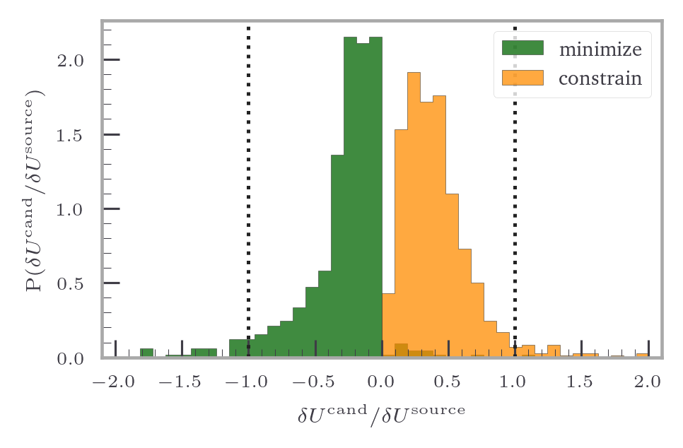
Figure A3: Perturbing entire large pockets. Histogram of energy changes during loading and relaxation for protein-derived networks. Here we constrain the predicted large (i.e. entire) pockets instead of sub-sampling beads comprising them.

To eliminate any further concerns regarding pocket-size effects, we take a closer look at the true source pocket itself. Indeed, we did not scan in Sec. A large entire pockets, but instead generated various combinations of possible ligand-binding sites within these. The true source pocket is somewhat larger than these considered combinations, see Fig. A2. As we throughout always divided by the number of perturbed beads, their actual number (i.e. size) should in principle have no effect.

However, a further control is advisable to rule out other possible pocket-size effects occur. Equivalently to the sampling performed within the larger (predicted) binding-pocket candidates, we therefore also inspect the source pocket by scanning across all combinations of bead triplets within the pocket.

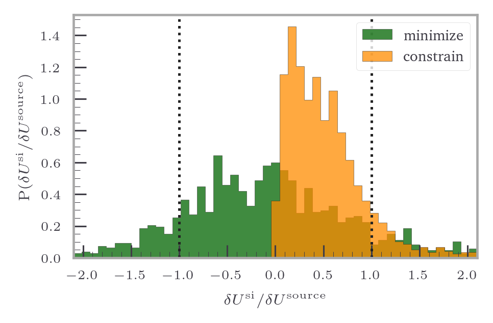
Figure A4: Perturbing only subsets of large pockets. Histogram of energy changes for protein-derived networks, where we sub-sample large source pocket candidates.

In general the fact that beads in a source pocket bind the ligand does not imply that all of them are equally important for transmitting the allosteric signal. It is just as conceivable that only a subset thereof is actually responsible for loading the stiff collective springs. This is also how we interpret the results of sub-sampling the true source pockets shown in Fig. A4, where we see a significant difference in the distribution of energy changes during the relaxation step of the true with respect to the other pocket candidates. Notably, however, we recover the familiar trend for the energy change during loading. This implies that indeed not all beads in the true source pocket contribute equally/comparably to the loading. Rather there exists a subset of critically important beads within the source pockets, which account for the major energy input during loading. We observe that as long as we do not constrain these critical beads and instead the beads connected to these critical ones, the energy does not increase immediately during the loading step, but instead in the following minimization steps, that is, when the critical beads follow. In this respect, the relaxation movements of critical beads compensate for the absence of a large/efficient loading of non-critical beads in the source pocket.

Appendix B Construction and training of artificial allosteric pseudoproteins

Many alternative methods are available for designing and training allosteric networks. In our work we generalize and optimize the method developed by Flechsig [61]. We first “grow” the networks to resemble folded coarse-grained proteins. The first bead is positioned at the origin and afterwards the following steps are iterated until the desired total number of beads $N$ is reached: Each subsequent bead is placed on the surface of a $3-$dimensional sphere centered at the location of the previously positioned bead with a radius $d_{\rm min}$ under the constraint that the distance to all other beads is also above $d_{\rm min}$. Two other constraints are imposed: First, all beads must lie within a large sphere of radius $d_{\rm big}$ such that a globular shape is attained. Second, the volume enclosed by two smaller spheres of $d_{\rm small}$ which intersect the large sphere is left unpopulated, such that two “binding pockets” emerge. For a subset of networks we combine two of the grown structures by overlapping them and removing all beads that thereafter lie closer together than $d_{\rm min}$. Detailed parameters for the grown networks are given in Table A2. The source and target pocket, respectively, are comprised of two or three beads which are selected by hand.

These grown networks are trained to exhibit a long-range allosteric effect consisting of an input and an output. A ligand-binding event that closes the source pocket is mimicked by pulling the beads of the source pocket towards their local center of mass—we refer to this as the input. Conversely, we refer to the opening or closing of the target binding pocket (depending on the variant being trained) as the output. The full nonlinear response of the network to the input perturbation of the source pocket is described below.

We quantify the state of the source ($A=S$) and target ($A=T$) pocket, respectively, via the squared radius of gyration, defined as

$$r^{2}_{\rm gyr}(A)\equiv\frac{1}{N_{A}}\sum_{i\in A}\Big{(}\mathbf{r}_{i}-\sum_{j\in A}\mathbf{r}_{j}/N_{A}\Big{)}^{2}$$ (A1)

We train the networks according to their response to the input perturbation in an open-system Monte Carlo (MC) fashion. That is, beads can change their resting position $\mathbf{r}_{i}^{0}$ and new beads can be created or existing ones removed. The algorithm is inspired by the principle of natural evolution, corresponding to mutations that change amino acids at a given position in the sequence, or more drastic insertions [135] and deletions [136], respectively.

First, one of the three possible steps (move, delete, insert) is randomly chosen with probabilities $1/2,1/4$ and $1/4$, respectively, and the response of the mutated network determined. If the response at the target site has improved according to the variant trained (i.e. $r^{2}_{\rm gyr}(T)$ has increased or decreased for a symmetric and antisymmetric response, respectively), the change is accepted with probability one and otherwise with probability $\exp(-|\Delta r_{\rm gyr}(T)|)$, where $\Delta r_{\rm gyr}(T)\equiv r^{\rm init}_{\rm gyr}(T)-r^{\rm fin}_{\rm gyr}(T)$ is the change in target-pocket size during the response. The exponent prevents too large unwanted changed while concurrently allowing to avoid getting stuck in local favorable but suboptimal minima. Less than $10^{3}$ MC steps were required to incorporate the desired effect into the networks.

Notably, to remove any potential bias in the above method, we also considered networks derived from the random “dense packed-spheres” algorithm [137]. This yielded structures that are closer to those in [43, 44]. However, we subsequently subjected these structures to the same evolutionary training, since simple flipping or pruning of bonds is not possible within the standard ENM framework following Tirion [70]. In total, we generated a set of 30 artificial ENMs trained to display a specific response.

Appendix C Binding-pocket candidates in artificial networks

In the case of artificial networks we identify binding-pocket candidates as pairs or triplets of beads resembling a simple binding pocket. We impose (i) that binding-pocket candidates must be accessible to hypothetical ligands (i.e. that they must lie on the surface of the network) and (ii) that they actually form a pocket, that is, that is the lines connecting the respective beads do not cut through the bulk of the network. Both constraints embody the definition of the surface of a network. As opposed to atomically detailed proteins above, defining the surface of a network (i.e. the concave hull of a cloud of points in 3 dimensions) is neither mathematically nor intuitively well posed. Many different shapes may envelop the respective structures.

We chose a unique definiton of “the surface” as the surface that emerges by growing a sphere around each of the beads such that a coherent solid body emerges. This fused-spheres object consistently defines a surface of the network that actually is quite similar to the definition of the SAS area for proteins (see Fig. A5). We declare beads that belong to spheres participating in this outer shared surface as surface beads and the remaining ones as interior beads.

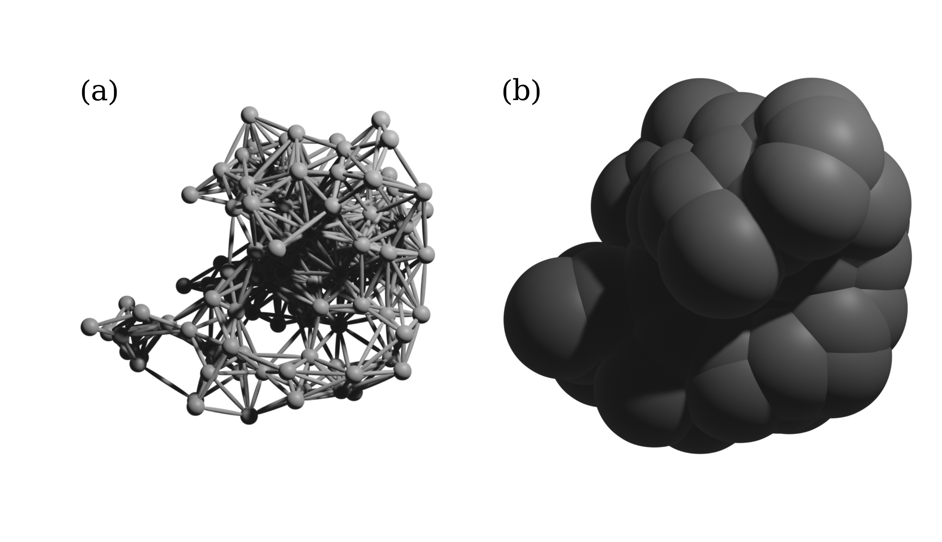
Figure A5: We define the surface beads of a network (a) as those beads that contribute to the shared surface after growing the radii of the beads (b). Potential binding pockets are selected from this set of beads.

Pocket pairs and triplets are now selected from the set of surface beads. The condition that binding pockets must lie on the outer surface rules out “implausible ligand” effects, enforced as follows. Out of all possible combinations of pars of surface beads and triplets we only consider those whose direct connecting lines do not cut any of the interior beads. In addition, we omit pairs if they are direct neighbors or if their distance is above a certain threshold value.

Table A2: Overview of parameters of analyzed pseudoproteins; $r_{c}$ is the cutoff length (in natural, dimensionless units), $N$ the total number of beads, $N_{T}$ and $N_{S}$ the number of beads composing the target and source pocket, respectively, and $N_{\text{sp}}$ and $N_{\text{st}}$ the numbers of pocket candidates, bead pairs and triplets, respectively.

ID	variant	$r_{c}$	$N$	$N_{T}$	$N_{S}$	$N_{\rm sp}$	$N_{\rm st}$	origin
1	anti	1.63	120	2	2	206	206	packed spheres
2	symm	6.0	95	3	3	376	376	pseudoprotein
3	anti	6.0	94	3	3	295	295	pseudoprotein
4	symm	6.0	89	3	3	224	224	pseudoprotein
5	symm	6.0	142	3	3	201	201	pseudoprotein
6	anti	6.0	142	3	3	309	309	pseudoprotein
7	anti	6.0	180	3	3	530	530	pseudoprotein
8	symm	6.0	93	3	3	461	461	pseudoprotein
9	anti	6.0	154	3	3	315	315	pseudoprotein
10	symm	6.0	100	3	3	540	540	pseudoprotein
11	symm	6.0	99	3	3	401	401	pseudoprotein
12	anti	6.0	94	3	3	294	294	pseudoprotein
13	symm	6.0	93	3	3	535	535	pseudoprotein
14	symm	6.0	147	3	2	495	495	pseudoprotein
15	symm	6.0	94	3	3	330	330	pseudoprotein
16	symm	6.0	99	3	3	332	332	pseudoprotein
17	symm	6.0	154	3	3	465	465	pseudoprotein
18	anti	6.0	89	3	3	288	288	pseudoprotein
19	anti	6.0	93	3	3	461	461	pseudoprotein
20	anti	6.0	95	3	3	317	317	pseudoprotein
21	anti	6.0	99	3	3	400	400	pseudoprotein
22	anti	6.0	100	3	3	480	480	pseudoprotein
23	symm	6.0	135	3	3	571	571	pseudoprotein
24	symm	6.0	88	3	3	187	187	pseudoprotein
25	symm	6.0	87	3	3	244	244	pseudoprotein
26	symm	6.0	169	3	3	386	386	pseudoprotein
27	anti	6.0	147	3	2	427	427	pseudoprotein
28	anti	6.0	99	3	3	353	353	pseudoprotein
29	anti	6.0	87	3	3	234	234	pseudoprotein
30	anti	6.0	169	3	3	382	382	pseudoprotein
1F	anti	9.0	200	2	2	845	2204	[61]
2F	symm	9.0	200	2	2	892	2691	[61]

Appendix D Removing rigid-body motions

The Hessian is singular, its nullspace $\mathcal{N}({\textsf{H}})$ is spanned by the vectors describing infinitesimal rigid body motions. Depending on the number of constraints, the solution of Eq. (7) is not necessarily unique, i.e. the system is underdetermined. The following simple algebraic trick solves this problem.

Consider the square matrix ${\textsf{M}}\in\mathbbm{R}^{m\times m}$ which does not have full rank $r$, its nullity being $n$, such that $n+r=m$. The nullspace is $\mathcal{N}({\textsf{M}})$ with dimension $n$ and its row space (or range) is $\mathcal{R}({\textsf{M}}^{T})$ with dimension $r$. All vectors in $\mathcal{N}({\textsf{M}})$ are orthogonal to all vectors in $\mathcal{R}({\textsf{M}}^{T})$ Therefore, if we add a matrix given by an outer product of a basis vector $\mathbf{x}$ from the nullspace to M, i.e. $\tilde{{\textsf{M}}}\equiv{\textsf{M}}+\mathbf{x}\otimes\mathbf{x}^{T}$, we increase the rank of M by one. Applying this for each basis vector of $\mathcal{N}({\textsf{M}})$ gives M full rank [139]. This, however, does not change any result where the matrix is applied to a vector $\mathbf{y}$ from the row space $\mathcal{R}({\textsf{M}}^{T})$, since

$$\tilde{{\textsf{M}}}\mathbf{y} \equiv {\textsf{M}}\mathbf{y}+\mathbf{x}\otimes\mathbf{x}^{T}\mathbf{y}$$ (A2)

$$= {\textsf{M}}\mathbf{y}+(\mathbf{x}^{T}\mathbf{y})\mathbf{y}={\textsf{M}}\mathbf{x},\quad\forall\mathbf{x}\in\mathcal{N}({\textsf{M}}).$$

We apply this rank extension only to the sub-block S containing free beads $\mathbf{s}$ in Eq. (4). Constraining the positions of beads in $\mathbf{c}$ would otherwise conflict the constrained degrees of freedom. The resulting matrix has full rank, rendering the linear system (7) uniquely solvable. The solution thus by construction does not contain any rigid body motions.

It is even possible to identify the basis vectors of the nullspace explicitly in terms of Cartesian basis vectors $\mathbf{e}_{x},\mathbf{e}_{y},\mathbf{e}_{z}$. In the 3-dimensional Cartesian basis the vectors generating translations of a body with $N$ beads can be written as $3N$-dimensional supervectors, $\bm{\tau}(\alpha)=(\mathbf{e}_{\alpha},\ldots,\mathbf{e}_{\alpha})^{T}$, for $\alpha=x,y,z$. Given the position of beads $\mathbf{R}=(\mathbf{r}_{1},\ldots,\mathbf{r}_{N})^{T}$ the basis vectors $\bm{\rho}(\alpha)$ generating infinitesimal rotations of the network can be constructed as $\bm{\rho}(\alpha)=(\mathbf{e}_{\alpha}\times\mathbf{r}_{1},\ldots,\mathbf{e}_{\alpha}\times\mathbf{r}_{N})^{T}$. Both methods are equivalent whereby the second method is faster. If we constrain more than two beads (essentially always true for the binding sites in proteins) the removal of rigid body motions can be omitted entirely, speeding up the algorithm tremendously.

Appendix E ROC curves for energy change during constraining

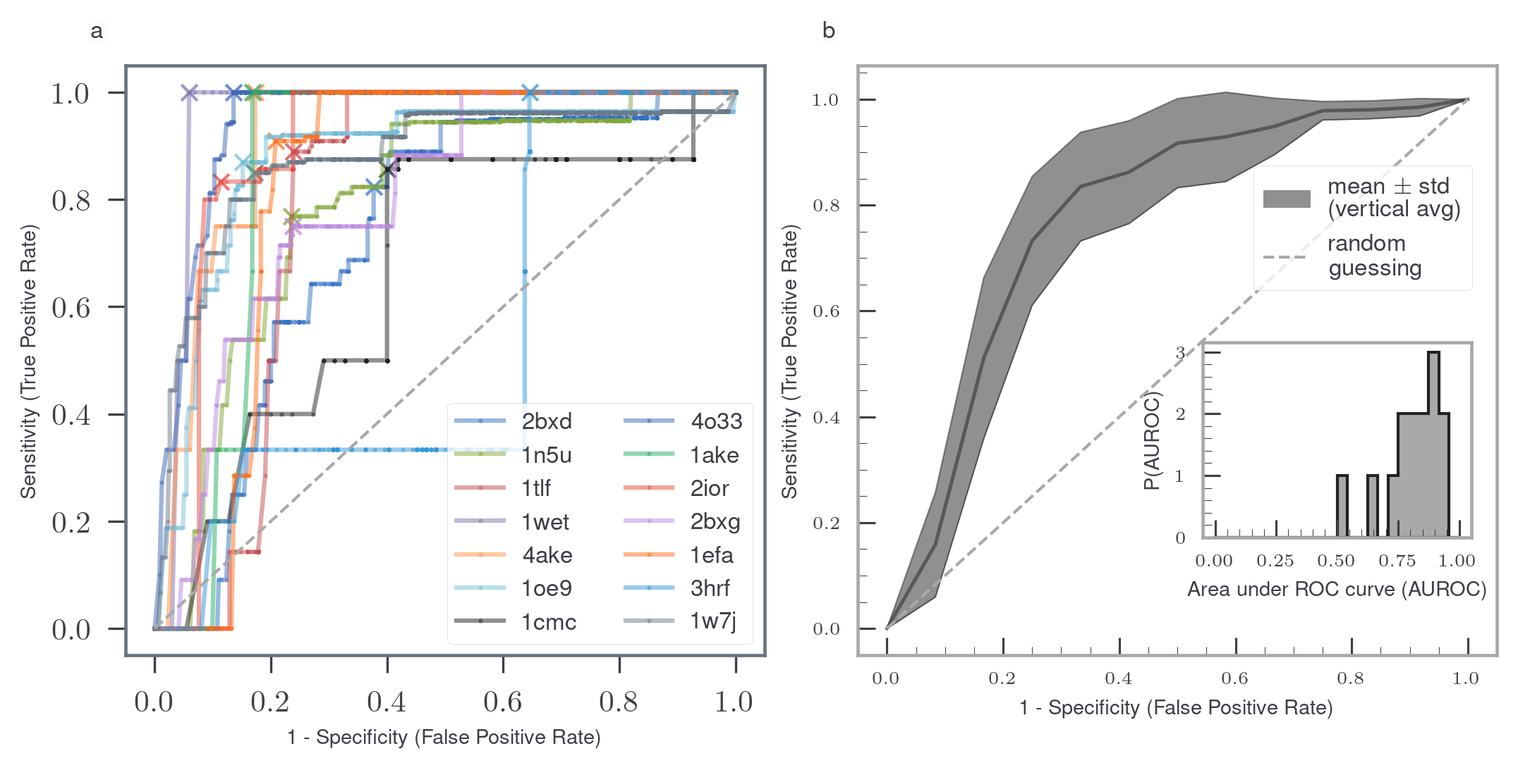
Figure A6: For an explanation refer to Fig. 6. Results are similar on average but with a larger spread.

For completeness, we also rank source-pocket candidates according to how much energy is taken up during the constraining step $\delta U(\delta\mathbf{c})$. As shown in Fig A6, the results are similar on average, but show a larger variance.

Appendix F Finding avoided crossings

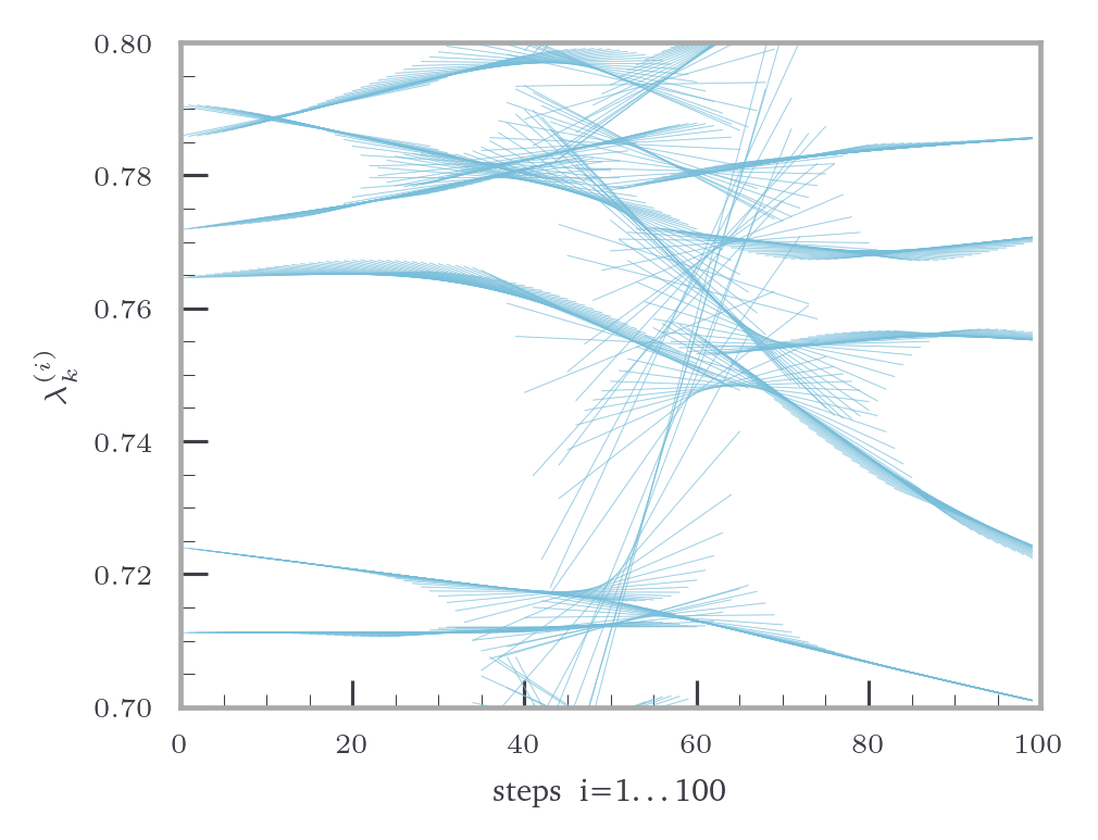
Figure A7: Intersection points of consecutive tangents to eigenvalues. An example illustrating the motion of mid-point tangents in Eq. (15) for a set of eigenvalues during the response of one generic pseudoprotein.

As detailed in Sec. III.1, we determine mid-point tangents $T_{l}(k)$ for all points $k$ along the eigenvalue curves during the response (see Eq. (15)), whereby we exclude the first and last point of each curve. An avoided crossing between a given pair of eigenvalues $l$ and $l+1$ at step $k$ occurs when the intersection point first diverges towards $+\infty$ as a function of $k$ and subsequently re-enters from $-\infty$. This is illustrated in Fig. A7. The “precise” location of an intersection is determined on the basis of a sign-change of $\omega_{l+1}(k)-\omega_{l}(k)$. Only instances where the crossing occurs first from above ($+\to-$) and then from below ($-\to+$) are considered.

References

- Changeux and Edelstein [2005] J.-P. Changeux and S. J. Edelstein, Allosteric mechanisms of signal transduction, Science 308, 1424–1428 (2005).
- Tsai et al. [2008] C.-J. Tsai, A. del Sol, and R. Nussinov, Allostery: Absence of a change in shape does not imply that allostery is not at play, J. Mol. Biol. 378, 1–11 (2008).
- McLeish et al. [2018] T. McLeish, C. Schaefer, and A. C. von der Heydt, The ‘allosteron’ model for entropic allostery of self-assembly, Phil. Trans. Roy. Soc. B 373, 20170186 (2018).
- Cooper and Dryden [1984] A. Cooper and D. T. F. Dryden, Allostery without conformational change: A plausible model, Eur. Biophys. J. 11, 103–109 (1984).
- Modi et al. [2022] T. Modi, M. Heyden, and S. B. Ozkan, Vibrational density of states capture the role of dynamic allostery in protein evolution, Biophys. J. 121, 456a (2022).
- Mccammon et al. [1976] J. A. Mccammon, B. R. Gelin, M. Karplus, and P. G. Wolynes, The hinge-bending mode in lysozyme, Nature 262, 325–326 (1976).
- Daily and Gray [2007] M. D. Daily and J. J. Gray, Local motions in a benchmark of allosteric proteins, Proteins 67, 385–399 (2007).
- Zheng et al. [2006] W. Zheng, B. R. Brooks, and D. Thirumalai, Low-frequency normal modes that describe allosteric transitions in biological nanomachines are robust to sequence variations, Proc. Natl. Acad. Sci. 103, 7664–7669 (2006).
- Laskowski et al. [2009] R. A. Laskowski, F. Gerick, and J. M. Thornton, The structural basis of allosteric regulation in proteins, FEBS Lett. 583, 1692–1698 (2009).
- Selvaratnam et al. [2011] R. Selvaratnam, S. Chowdhury, B. VanSchouwen, and G. Melacini, Mapping allostery through the covariance analysis of nmr chemical shifts, Proc. Natl. Acad. Sci. 108, 6133–6138 (2011).
- Mitchell et al. [2016] M. R. Mitchell, T. Tlusty, and S. Leibler, Strain analysis of protein structures and low dimensionality of mechanical allosteric couplings, Proc. Natl. Acad. Sci. 113, 10.1073/pnas.1609462113 (2016).
- Bozovic et al. [2020] O. Bozovic, B. Jankovic, and P. Hamm, Sensing the allosteric force, Nat. Commun. 11, 10.1038/s41467-020-19689-7 (2020).
- Kipnis et al. [2007] Y. Kipnis, N. Papo, G. Haran, and A. Horovitz, Concerted atp-induced allosteric transitions in groel facilitate release of protein substrate domains in an all-or-none manner, Proc. Natl. Acad. Sci. 104, 3119–3124 (2007).
- Frank et al. [2011] G. A. Frank, A. Horovitz, and G. Haran, Fluorescence correlation spectroscopy and allostery: The case of groel, Allostery , 205–216 (2011).
- Piwonski et al. [2012] H. M. Piwonski, M. Goomanovsky, D. Bensimon, A. Horovitz, and G. Haran, Allosteric inhibition of individual enzyme molecules trapped in lipid vesicles, Proc. Natl. Acad. Sci. 109, 10.1073/pnas.1116670109 (2012).
- Mazal et al. [2019] H. Mazal, M. Iljina, Y. Barak, N. Elad, R. Rosenzweig, P. Goloubinoff, I. Riven, and G. Haran, Tunable microsecond dynamics of an allosteric switch regulate the activity of a aaa+ disaggregation machine, Nat. Commun. 10, 10.1038/s41467-019-09474-6 (2019).
- Scheerer et al. [2023] D. Scheerer, B. V. Adkar, S. Bhattacharyya, D. Levy, M. Iljina, I. Riven, O. Dym, G. Haran, and E. I. Shakhnovich, Allosteric communication between ligand binding domains modulates substrate inhibition in adenylate kinase, Proc. Natl. Acad. Sci. 120, 10.1073/pnas.2219855120 (2023).
- Rosenblum et al. [2019] G. Rosenblum, N. Elad, F. Wiggers, and H. Hofmann, Observation of allosteric signaling through dna with single-molecule fret and cryo-em, Biophys. J. 116, 214a (2019).
- Rosenblum et al. [2021] G. Rosenblum, N. Elad, H. Rozenberg, F. Wiggers, J. Jungwirth, and H. Hofmann, Allostery through dna drives phenotype switching, Nat. Commun. 12, 10.1038/s41467-021-23148-2 (2021).
- Laine et al. [2012] E. Laine, C. Auclair, and L. Tchertanov, Allosteric communication across the native and mutated kit receptor tyrosine kinase, PLoS Comput. Biol. 8, e1002661 (2012).
- Weinkam et al. [2013] P. Weinkam, Y. C. Chen, J. Pons, and A. Sali, Impact of mutations on the allosteric conformational equilibrium, J. Mol. Biol. 425, 647 (2013).
- Smith et al. [2016] C. A. Smith, D. Ban, S. Pratihar, K. Giller, M. Paulat, S. Becker, C. Griesinger, D. Lee, and B. L. de Groot, Allosteric switch regulates protein–protein binding through collective motion, Proc. Natl. Acad. Sci. 113, 3269–3274 (2016).
- Zhou et al. [2017] B. Zhou, P. J. Hogg, and F. Gräter, One-way allosteric communication between the two disulfide bonds in tissue factor, Biophys. J. 112, 78 (2017).
- Buchenberg et al. [2017] S. Buchenberg, F. Sittel, and G. Stock, Time-resolved observation of protein allosteric communication, Proc. Natl. Acad. Sci. 114, 10.1073/pnas.1707694114 (2017).
- Elbahnsi and Delemotte [2021] A. Elbahnsi and L. Delemotte, Structure and sequence-based computational approaches to allosteric signal transduction: Application to electromechanical coupling in voltage-gated ion channels, J. Mol. Biol. 433, 167095 (2021).
- Franz et al. [2023] F. Franz, R. Tapia-Rojo, S. Winograd-Katz, R. Boujemaa-Paterski, W. Li, T. Unger, S. Albeck, C. Aponte-Santamaria, S. Garcia-Manyes, O. Medalia, B. Geiger, and F. Gräter, Allosteric activation of vinculin by talin, Nat. Commun. 14, 10.1038/s41467-023-39646-4 (2023).
- Leitner and John E. Straub [2009] D. M. Leitner and J. E. John E. Straub, Proteins: Energy, Heat and Signal Flow (CRC Press, 2009).
- Stock and Hamm [2018] G. Stock and P. Hamm, A non-equilibrium approach to allosteric communication, Phil. Trans. Roy. Soc. B 373, 20170187 (2018).
- Amor et al. [2016] B. R. C. Amor, M. T. Schaub, S. N. Yaliraki, and M. Barahona, Prediction of allosteric sites and mediating interactions through bond-to-bond propensities, Nat. Commun. 7, 12477 (2016).
- del Sol et al. [2006] A. del Sol, H. Fujihashi, D. Amoros, and R. Nussinov, Residues crucial for maintaining short paths in network communication mediate signaling in proteins, Mol. Sys. Biol. 2, 10.1038/msb4100063 (2006).
- Kaya et al. [2013] C. Kaya, A. Armutlulu, S. Ekesan, and T. Haliloglu, Mcpath: Monte carlo path generation approach to predict likely allosteric pathways and functional residues, Nucl. Acids Res. 41, W249–W255 (2013).
- Greener et al. [2017] J. G. Greener, I. Filippis, and M. J. Sternberg, Predicting protein dynamics and allostery using multi-protein atomic distance constraints, Structure 25, 546–558 (2017).
- Atilgan et al. [2007] A. R. Atilgan, D. Turgut, and C. Atilgan, Screened nonbonded interactions in native proteins manipulate optimal paths for robust residue communication, Biophys. J. 92, 3052 (2007).
- Mitternacht and Berezovsky [2011] S. Mitternacht and I. N. Berezovsky, Coherent conformational degrees of freedom as a structural basis for allosteric communication, PLoS Comput. Biol. 7, e1002301 (2011).
- Garcia et al. [2012] H. Garcia, A. Sanchez, J. Boedicker, M. Osborne, J. Gelles, J. Kondev, and R. Phillips, Operator sequence alters gene expression independently of transcription factor occupancy in bacteria, Cell Rep. 2, 150–161 (2012).
- Kim et al. [2013] S. Kim, E. Broströmer, D. Xing, J. Jin, S. Chong, H. Ge, S. Wang, C. Gu, L. Yang, Y. Q. Gao, X. dong Su, Y. Sun, and X. S. Xie, Probing allostery through dna, Science 339, 816 (2013).
- Peselis et al. [2015] A. Peselis, A. Gao, and A. Serganov, Cooperativity, allostery and synergism in ligand binding to riboswitches, Biochimie 117, 100–109 (2015).
- Hamilton et al. [2023] S. Hamilton, T. Modi, P. Sulc, and S. B. Ozkan, Rna-induced allosteric coupling drives viral capsid assembly in the single-stranded rna virus bacteriophage ms2, Biophys. J. 122, 48a–49a (2023).
- Walker et al. [2020] A. S. Walker, W. P. Russ, R. Ranganathan, and A. Schepartz, Rna sectors and allosteric function within the ribosome, Proc. Natl. Acad. Sci. 117, 19879–19887 (2020).
- Nussinov and Tsai [2013] R. Nussinov and C.-J. Tsai, Allostery in disease and in drug discovery, Cell 153, 293–305 (2013).
- Chatzigoulas and Cournia [2021] A. Chatzigoulas and Z. Cournia, Rational design of allosteric modulators: Challenges and successes, WIREs Comput. Mol. Sci. 11, 10.1002/wcms.1529 (2021).
- Goodrich et al. [2015] C. P. Goodrich, A. J. Liu, and S. R. Nagel, The principle of independent bond-level response: Tuning by pruning to exploit disorder for global behavior, Phys. Rev. Lett. 114, 225501 (2015).
- Yan et al. [2017] L. Yan, R. Ravasio, C. Brito, and M. Wyart, Architecture and coevolution of allosteric materials, Proc. Natl. Acad. Sci. 114, 2526–2531 (2017).
- Rocks et al. [2017] J. W. Rocks, N. Pashine, I. Bischofberger, C. P. Goodrich, A. J. Liu, and S. R. Nagel, Designing allostery-inspired response in mechanical networks, Proc. Natl. Acad. Sci. 114, 2520–2525 (2017).
- Kim et al. [2019] J. Z. Kim, Z. Lu, S. H. Strogatz, and D. S. Bassett, Conformational control of mechanical networks, Nat. Phys. 15, 714–720 (2019).
- Kim et al. [2022] J. Z. Kim, Z. Lu, A. S. Blevins, and D. S. Bassett, Nonlinear dynamics and chaos in conformational changes of mechanical metamaterials, Phys. Rev. X 12, 011042 (2022).
- Rocks et al. [2021a] J. W. Rocks, A. J. Liu, and E. Katifori, Hidden topological structure of flow network functionality, Phys. Rev. Lett. 126, 028102 (2021a).
- Bohr et al. [1904] C. Bohr, K. A. Hasselbalch, and A. Krogh, Ueber einen in biologischer beziehung wichtigen einfluss, den die kohlensäurespannung des blutes auf dessen sauerstoffbindung übt1, Acta Physiol. 16, 402 (1904).
- Monod et al. [1965] J. Monod, J. Wyman, and J.-P. Changeux, On the nature of allosteric transitions: A plausible model, J, Mol. Biol. 12, 88 (1965).
- Koshland et al. [1966] D. E. Koshland, G. Némethy, and D. Filmer, Comparison of experimental binding data and theoretical models in proteins containing subunits, Biochemistry 5, 365–385 (1966).
- Eigen [1968] M. Eigen, New looks and outlooks on physical enzymology, Quart. Rev. Biophys. 1, 3–33 (1968).
- Ascenzi and Fasano [2010] P. Ascenzi and M. Fasano, Allostery in a monomeric protein: The case of human serum albumin, Biophys. Chem. 148, 16 (2010).
- Cuendet et al. [2016] M. A. Cuendet, H. Weinstein, and M. V. LeVine, The allostery landscape: Quantifying thermodynamic couplings in biomolecular systems, J. Chem. Theory Comput. 12, 5758–5767 (2016).
- Hilser et al. [2012] V. J. Hilser, J. O. Wrabl, and H. N. Motlagh, Structural and energetic basis of allostery, Annu. Rev. Biophys. 41, 585 (2012).
- Motlagh et al. [2014] H. N. Motlagh, J. O. Wrabl, J. Li, and V. J. Hilser, The ensemble nature of allostery, Nature 508, 331–339 (2014).
- Cui and Karplus [2008] Q. Cui and M. Karplus, Allostery and cooperativity revisited, Protein Science 17, 1295 (2008).
- Kar et al. [2010] G. Kar, O. Keskin, A. Gursoy, and R. Nussinov, Allostery and population shift in drug discovery, Curr. Opin. Pharmacol. 10, 715 (2010).
- Thirumalai et al. [2019] D. Thirumalai, C. Hyeon, P. I. Zhuravlev, and G. H. Lorimer, Symmetry, rigidity, and allosteric signaling: From monomeric proteins to molecular machines, Chem. Rev. 119, 6788–6821 (2019).
- Hofmann [2023] H. Hofmann, All over or overall – do we understand allostery?, Curr. Opin. Struct. Biol. 83, 102724 (2023).
- Wodak [2019] S. J. e. a. Wodak, Allostery in its many disguises: From theory to applications, Structure 27, 566–578 (2019).
- Flechsig [2017] H. Flechsig, Design of elastic networks with evolutionary optimized long-range communication as mechanical models of allosteric proteins, Biophys. J. 113, 558–571 (2017).
- Fenton [2008] A. W. Fenton, Allostery: an illustrated definition for the ‘second secret of life’, Trends Biochem. Sci. 33, 420–425 (2008).
- Miyashita et al. [2003] O. Miyashita, J. N. Onuchic, and P. G. Wolynes, Nonlinear elasticity, proteinquakes, and the energy landscapes of functional transitions in proteins, Proc. Natl. Acad. Sci. 100, 12570–12575 (2003).
- Togashi and Mikhailov [2007] Y. Togashi and A. S. Mikhailov, Nonlinear relaxation dynamics in elastic networks and design principles of molecular machines, Proc. Natl. Acad. Sci. 104, 8697–8702 (2007).
- Togashi et al. [2010] Y. Togashi, T. Yanagida, and A. S. Mikhailov, Nonlinearity of mechanochemical motions in motor proteins, PLoS Comput. Biol. 6, e1000814 (2010).
- Yan et al. [2018] L. Yan, R. Ravasio, C. Brito, and M. Wyart, Principles for optimal cooperativity in allosteric materials, Biophys. J. 114, 2787–2798 (2018).
- Poma et al. [2018] A. B. Poma, M. S. Li, and P. E. Theodorakis, Generalization of the elastic network model for the study of large conformational changes in biomolecules, Phys. Chem. Chem. Phys. 20, 1463 (2018).
- Ghuman et al. [2005] J. Ghuman, P. A. Zunszain, I. Petitpas, A. A. Bhattacharya, M. Otagiri, and S. Curry, Structural basis of the drug-binding specificity of human serum albumin, J. Mol. Biol. 353, 38 (2005).
- Tian et al. [2018] W. Tian, C. Chen, X. Lei, J. Zhao, and J. Liang, Castp 3.0: computed atlas of surface topography of proteins, Nucl. Acids Res. 46, W363 (2018).
- Tirion [1996] M. M. Tirion, Large amplitude elastic motions in proteins from a single-parameter, atomic analysis, Phys. Rev. Lett. 77, 1905–1908 (1996).
- Zheng and Brooks [2005] W. Zheng and B. Brooks, Identification of Dynamical Correlations within the Myosin Motor Domain by the Normal Mode Analysis of an Elastic Network Model, J. Mol. Bio. 346, 745 (2005).
- Ravasio et al. [2019] R. Ravasio, S. M. Flatt, L. Yan, S. Zamuner, C. Brito, and M. Wyart, Mechanics of allostery: Contrasting the induced fit and population shift scenarios, Biophys. J. 117, 1954 (2019).
- Gerstein and Krebs [1998] M. Gerstein and W. Krebs, A database of macromolecular motions, Nucl. Acids Res. 26, 4280 (1998).
- Taylor et al. [2014] D. Taylor, G. Cawley, and S. Hayward, Quantitative method for the assignment of hinge and shear mechanism in protein domain movements, Bioinformatics 30, 3189 (2014).
- Liu [2021] A. Liu, Doing “statistical mechanics” with big data: Understanding protein allostery, Bull. Am. Phys. Soc. (2021).
- Haliloglu et al. [1997] T. Haliloglu, I. Bahar, and B. Erman, Gaussian dynamics of folded proteins, Phys. Rev. Lett. 79, 3090–3093 (1997).
- Sanejouand [2013] Y.-H. Sanejouand, Elastic network models: Theoretical and empirical foundations, in Biomolecular Simulations: Methods and Protocols, edited by L. Monticelli and E. Salonen (Humana Press, 2013) p. 601–616.
- Kondrashov et al. [2007] D. A. Kondrashov, A. W. Van Wynsberghe, R. M. Bannen, Q. Cui, and G. N. Phillips Jr, Protein structural variation in computational models and crystallographic data, Structure, Structure 15, 169 (2007).
- Kundu et al. [2002] S. Kundu, J. S. Melton, D. C. Sorensen, and G. N. Phillips Jr, Dynamics of proteins in crystals: comparison of experiment with simple models, Biophysical Journal, Biophysical journal 83, 723 (2002).
- Soheilifard et al. [2008] R. Soheilifard, D. E. Makarov, and G. J. Rodin, Critical evaluation of simple network models of protein dynamics and their comparison with crystallographic b-factors, Phys. Biol. 5, 026008 (2008).
- Ansari et al. [1992] A. Ansari, C. M. Jones, E. R. Henry, J. Hofrichter, and W. A. Eaton, The role of solvent viscosity in the dynamics of protein conformational changes, Science 256, 1796–1798 (1992).
- Atilgan et al. [2010] C. Atilgan, Z. Gerek, S. Ozkan, and A. Atilgan, Manipulation of conformational change in proteins by single-residue perturbations, Biophys. J. 99, 933–943 (2010).
- Atilgan and Atilgan [2009] C. Atilgan and A. R. Atilgan, Perturbation-response scanning reveals ligand entry-exit mechanisms of ferric binding protein, PLoS Comput. Biol. 5, e1000544 (2009).
- Zheng and Doniach [2003] W. Zheng and S. Doniach, A comparative study of motor-protein motions by using a simple elastic-network model, Proc. Natl. Acad. Sci. 100, 13253 (2003).
- Note [1] According to the fluctuation-dissipation theorem we have for small that and accordingly the linear response to a small force , , follows. Equivalently, one may also impose a constraint as we do and solve for the force on, and displacements of, the free beads [43, 82].
- Trotter [1959] H. F. Trotter, On the product of semi-groups of operators, Proc. Amer. Math. Soc. 10, 545 (1959).
- Marcus [1980] R. A. Marcus, Molecular behavior in the quasi-periodic and stochastic regimes, Ann. N. Y. Acad. Sci. 357, 169 (1980).
- Noid et al. [1981] D. W. Noid, M. L. Koszykowski, and R. A. Marcus, Quasiperiodic and stochastic behavior in molecules, Annu. Rev. Phys. Chem. 32, 267 (1981).
- Uzer et al. [1983] T. Uzer, D. W. Noid, and R. A. Marcus, Uniform semiclassical theory of avoided crossings, J. Chem. Phys. 79, 4412–4425 (1983).
- Chirikov [1979] B. V. Chirikov, A universal instability of many-dimensional oscillator systems, Phys. Rep. 52, 263 (1979).
- Kabsch [1976] W. Kabsch, A solution for the best rotation to relate two sets of vectors, Acta Crystallogr. A 32, 922–923 (1976).
- Note [2] We have, setting , and , that and hence , and ; the squeeze bound (19\@@italiccorr) follows. Note also that rotations and translations preserve metric properties [140].
- Tee et al. [2018] W.-V. Tee, E. Guarnera, and I. N. Berezovsky, Reversing allosteric communication: From detecting allosteric sites to inducing and tuning targeted allosteric response, PLOS Comput. Biol. 14, e1006228 (2018).
- Ni et al. [2021] D. Ni, J. Wei, X. He, A. U. Rehman, X. Li, Y. Qiu, J. Pu, S. Lu, and J. Zhang, Discovery of cryptic allosteric sites using reversed allosteric communication by a combined computational and experimental strategy, Chem. Sci. 12, 464–476 (2021).
- Park et al. [2004] S. H. Park, J. M. Goo, and C.-H. Jo, Receiver operating characteristic (roc) curve: practical review for radiologists, Kor. J. Radiol. 5, 11 (2004).
- Fawcett [2006] T. Fawcett, An introduction to roc analysis, Pattern Recognit. Lett. 27, 861 (2006).
- Lockless and Ranganathan [1999] S. W. Lockless and R. Ranganathan, Evolutionarily conserved pathways of energetic connectivity in protein families, Science 286, 295 (1999).
- Schirmer and Evans [1990] T. Schirmer and P. R. Evans, Structural basis of the allosteric behaviour of phosphofructokinase, Nature 343, 140–145 (1990).
- Asthana et al. [2007] S. Asthana, M. Roytberg, J. Stamatoyannopoulos, and S. Sunyaev, Analysis of sequence conservation at nucleotide resolution, PLoS Comput. Biol. 3, e254 (2007).
- Ye et al. [2006] J. Ye, S. McGinnis, and T. L. Madden, BLAST: improvements for better sequence analysis, Nucl. Acids Res. 34, W6–W9 (2006).
- Sievers and Higgins [2013] F. Sievers and D. G. Higgins, Clustal omega, accurate alignment of very large numbers of sequences, Methods Mol. Biol. 1079, 105–116 (2013).
- Campitelli et al. [2020] P. Campitelli, T. Modi, S. Kumar, and S. B. Ozkan, The role of conformational dynamics and allostery in modulating protein evolution, Annu. Rev. Biophys. 49, 267–288 (2020).
- ben Avraham [1993] D. ben Avraham, Vibrational normal-mode spectrum of globular proteins, Phys. Rev. B 47, 14559 (1993).
- Nicolay and Sanejouand [2006] S. Nicolay and Y.-H. Sanejouand, Functional modes of proteins are among the most robust, Phys. Rev. Lett. 96, 078104 (2006).
- Na et al. [2018] H. Na, D. ben Avraham, and M. M. Tirion, Slow normal modes of proteins are accurately reproduced across different platforms, Phys. Biol. 16, 016003 (2018).
- Bartlett et al. [2002] G. J. Bartlett, C. T. Porter, N. Borkakoti, and J. M. Thornton, Analysis of catalytic residues in enzyme active sites, J. Mol. Biol. 324, 105 (2002).
- Yuan et al. [2003] Z. Yuan, J. Zhao, and Z.-X. Wang, Flexibility analysis of enzyme active sites by crystallographic temperature factors, Protein Eng. 16, 109–114 (2003).
- Anderson [1978] P. W. Anderson, Local moments and localized states, Science 201, 307–316 (1978).
- Zhang et al. [2020] Y. Zhang, P. Doruker, B. Kaynak, S. Zhang, J. Krieger, H. Li, and I. Bahar, Intrinsic dynamics is evolutionarily optimized to enable allosteric behavior, Curr. Opin. Struct. Biol. 62, 14–21 (2020).
- Tang et al. [2020] Q.-Y. Tang, T. S. Hatakeyama, and K. Kaneko, Functional sensitivity and mutational robustness of proteins, Phys. Rev. Res. 2, 033452 (2020).
- Granek and Klafter [2005] R. Granek and J. Klafter, Fractons in proteins: Can they lead to anomalously decaying time autocorrelations?, Phys. Rev. Lett. 95, 098106 (2005).
- Reuveni et al. [2008] S. Reuveni, R. Granek, and J. Klafter, Proteins: Coexistence of stability and flexibility, Phys. Rev. Lett. 100, 208101 (2008).
- Rocks et al. [2019] J. W. Rocks, H. Ronellenfitsch, A. J. Liu, S. R. Nagel, and E. Katifori, Limits of multifunctionality in tunable networks, Proc. Natil. Acad. Sci. 116, 2506–2511 (2019).
- Rocks et al. [2021b] J. W. Rocks, A. J. Liu, and E. Katifori, Hidden topological structure of flow network functionality, Phys. Rev. Lett. 126, 028102 (2021b).
- McLaughlin Jr et al. [2012] R. N. McLaughlin Jr, F. J. Poelwijk, A. Raman, W. S. Gosal, and R. Ranganathan, The spatial architecture of protein function and adaptation, Nature 491, 138–142 (2012).
- Shrake and Rupley [1973] A. Shrake and J. Rupley, Environment and exposure to solvent of protein atoms. lysozyme and insulin, J. Mol. Biol. 79, 351 (1973).
- Connolly [1983] M. L. Connolly, Solvent-accessible surfaces of proteins and nucleic acids, Science 221, 709–713 (1983).
- Delaunay [1934] B. Delaunay, Sur la sphère vide. a la mémoire de georges voronoï, Bull. Acad. Sci. USSR 6, 793 (1934).
- Edelsbrunner and Mücke [1994] H. Edelsbrunner and E. P. Mücke, Three-dimensional alpha shapes, ACM Trans. Graph. 13, 43–72 (1994).
- Edelsbrunner [1993] H. Edelsbrunner, The union of balls and its dual shape, Proceedings of the ninth annual symposium on Computational geometry 10.1145/160985.161139 (1993).
- Liang et al. [1998a] J. Liang, H. Edelsbrunner, P. Fu, P. V. Sudhakar, and S. Subramaniam, Analytical shape computation of macromolecules: I. molecular area and volume through alpha shape, Proteins 33, 1 (1998a).
- Liang et al. [1998b] J. Liang, H. Edelsbrunner, P. Fu, P. V. Sudhakar, and S. Subramaniam, Analytical shape computation of macromolecules: Ii. inaccessible cavities in proteins, Proteins 33, 18 (1998b).
- Shiau et al. [2006] A. K. Shiau, S. F. Harris, D. R. Southworth, and D. A. Agard, Structural analysis of e. coli hsp90 reveals dramatic nucleotide-dependent conformational rearrangements, Cell 127, 329 (2006).
- Rafferty et al. [1989] J. B. Rafferty, W. S. Somers, I. Saint-Girons, and S. E. Phillips, Three-dimensional crystal structures of escherichia coli met repressor with and without corepressor, Nature 341, 705 (1989).
- Schumacher et al. [1997] M. A. Schumacher, A. Glasfeld, H. Zalkin, and R. G. Brennan, The x-ray structure of the purr-guanine-purf operator complex reveals the contributions of complementary electrostatic surfaces and a water-mediated hydrogen bond to corepressor specificity and binding affinity, J. Biol. Chem. 272, 22648 (1997).
- Wardell et al. [2002] M. Wardell, Z. Wang, J. X. Ho, J. Robert, F. Ruker, J. Ruble, and D. C. Carter, The atomic structure of human methemalbumin at 1.9 Å, Biochem. Biophys. Res. Commun. 291, 813 (2002).
- Müller et al. [1996] C. Müller, G. Schlauderer, J. Reinstein, and G. E. Schulz, Adenylate kinase motions during catalysis: an energetic counterweight balancing substrate binding, Structure 4, 147 (1996).
- Müller and Schulz [1992] C. W. Müller and G. E. Schulz, Structure of the complex between adenylate kinase from escherichia coli and the inhibitor ap5a refined at 1.9 Å resolution: A model for a catalytic transition state, J. Mol. Biol. 224, 159 (1992).
- Coureux et al. [2003a] P.-D. Coureux, A. L. Wells, J. Ménétrey, C. M. Yengo, C. A. Morris, H. L. Sweeney, and A. Houdusse, A structural state of the myosin v motor without bound nucleotide, Nature 425, 419 (2003a).
- Coureux et al. [2003b] P.-D. Coureux, H. L. Sweeney, and A. Houdusse, Three myosin v structures delineate essential features of chemo-mechanical transduction, Nature 425, 419 (2003b).
- Chen et al. [2015] X. Chen, C. Zhao, X. Li, T. Wang, Y. Li, C. Cao, Y. Ding, M. Dong, L. Finci, J.-h. Wang, et al., Terazosin activates pgk1 and hsp90 to promote stress resistance, Nat. Chem. Biol. 11, 19 (2015).
- Hindie et al. [2009] V. Hindie, A. Stroba, H. Zhang, L. A. Lopez-Garcia, L. Idrissova, S. Zeuzem, D. Hirschberg, F. Schaeffer, T. J. Jørgensen, M. Engel, et al., Structure and allosteric effects of low-molecular-weight activators on the protein kinase pdk1, Nat. Chem. Biol. 5, 758 (2009).
- Bell and Lewis [2000] C. E. Bell and M. Lewis, A closer view of the conformation of the lac repressor bound to operator, Nat. Struct. Biol. 7, 209 (2000).
- Friedman et al. [1995] A. M. Friedman, T. O. Fischmann, and T. A. Steitz, Crystal structure of lac repressor core tetramer and its implications for dna looping, Science 268, 1721 (1995).
- King and Jukes [1969] J. L. King and T. H. Jukes, Non-darwinian evolution, Science 164, 788–798 (1969).
- Kimura [1968] M. Kimura, Evolutionary rate at the molecular level, Nature 217, 624–626 (1968).
- Baranau and Tallarek [2017] V. Baranau and U. Tallarek, Another resolution of the configurational entropy paradox as applied to hard spheres, J. Chem. Phys. 147, 224503 (2017).
- Note [3] Standard eigendecomposition routines are not ideal for a fast calculation of the eigenvectors that correspond to the 6 zero eigenvalues of H. Using a shift and invert spectral transformation from ARPACK [141], where we choose the number of eigenvalues we are interested in and provide a starting point for the search, is considerably faster. The corresponding implementation in scipy [142] does not always converge for eigenvalues that are of the same magnitude as the numerical precision (i.e. zero eigenvalues). We overcome this issue by adding a small noise to the matrix whose nullspace is to be determined.
- [139] A. Blázquez, V. Mantič, F. París, and J. Cañas, On the removal of rigid body motions in the solution of elastostatic problems by direct bem, Int. J. Num. Meth. Eng. 39, 4021.
- Fogolari et al. [2012] F. Fogolari, A. Corazza, P. Viglino, and G. Esposito, Fast structure similarity searches among protein models: efficient clustering of protein fragments, Algorithms Mol. Biol. 7, 10.1186/1748-7188-7-16 (2012).
- Lehoucq et al. [1998] R. B. Lehoucq, D. C. Sorensen, and C. Yang, Arpack users’ guide - solution of large-scale eigenvalue problems with implicitly restarted arnoldi methods, in Software, environments, tools (1998).
- Virtanen et al [2020] P. Virtanen et al, Scipy 1.0: fundamental algorithms for scientific computing in python, Nat. Methods 17, 261–272 (2020).