:
\theoremsep
\jmlrvolume
\firstpageno1
\jmlryear2023
\jmlrworkshopSymmetry and Geometry in Neural Representations
AMES: A Differentiable Embedding Space Selection Framework for Latent Graph Inference
Abstract
In real-world scenarios, although data entities may possess inherent relationships, the specific graph illustrating their connections might not be directly accessible. Latent graph inference addresses this issue by enabling Graph Neural Networks (GNNs) to operate on point cloud data, dynamically learning the necessary graph structure. These graphs are often derived from a latent embedding space, which can be modeled using Euclidean, hyperbolic, spherical, or product spaces. However, currently, there is no principled differentiable method for determining the optimal embedding space. In this work, we introduce the Attentional Multi-Embedding Selection (AMES) framework, a differentiable method for selecting the best embedding space for latent graph inference through backpropagation, considering a downstream task. Our framework consistently achieves comparable or superior results compared to previous methods for latent graph inference across five benchmark datasets. Importantly, our approach eliminates the need for conducting multiple experiments to identify the optimal embedding space. Furthermore, we explore interpretability techniques that track the gradient contributions of different latent graphs, shedding light on how our attention-based, fully differentiable approach learns to choose the appropriate latent space. In line with previous works, our experiments emphasize the advantages of hyperbolic spaces in enhancing performance. More importantly, our interpretability framework provides a general approach for quantitatively comparing embedding spaces across different tasks based on their contributions, a dimension that has been overlooked in previous literature on latent graph inference.
keywords:
Metric Learning, Latent Graph Inference, Neural Latent Geometry Search, Graph Neural Networks.1 Introduction
Graph Neural Networks (GNNs) efficiently leverage the geometric prior provided by the edge connections of graph-structured data through the utilization of an adjacency matrix. However, in many real-world applications, the graph connectivity structure may be incomplete, noisy, or even completely unknown. Utilizing latent graph inference enables the application of GNNs to point cloud data without requiring an input adjacency matrix, and it facilitates on-the-fly inference of the optimal graph structure for computation. Numerous studies have employed the Differentiable Graph Module (DGM) (Kazi et al., 2022) framework to infer latent graphs. This technique hinges on an embedding space, which is employed to deduce distances between nodes within the point cloud. Subsequently, connections are established based on these distances, ultimately shaping a graph. However, the task of selecting the most suitable embedding space is far from straightforward. Various approaches have explored the use of Euclidean space, hyperbolic spaces, spherical spaces, and stereographic projections of these spaces (Sáez de Ocáriz Borde et al., 2023b), as well as product spaces (Sáez de Ocáriz Borde et al., 2023c). Nevertheless, a principled approach for systematically selecting an optimal embedding space is lacking, particularly in a differentiable fashion. The latent geometry search procedure often relies on random search, which is computationally inefficient, particularly for product manifolds due to the multitude of possible manifold constructions.
In this study, we present an attention-based mechanism for latent graph inference: the Attentional Multi Embedding Selection (AMES) framework. Our approach effectively harnesses multiple latent candidate graphs derived from various latent spaces simultaneously. By employing an attention mechanism, it selects the most optimal latent representations while remaining differentiable. Consequently, this results in an end-to-end framework for the automated selection of latent embedding spaces in the context of latent graph inference. Importantly, we can achieve the same level of performance as existing latent graph inference methods with a single model, eliminating the need for experimental searches to find the optimal latent geometry. Furthermore, we put forward methods for interpretability that enable us to monitor the learning process of the selection mechanism and provide insights into its internal behavior.
2 Background
Geometric Deep Learning and Neural Latent Geometry Search. Geometric Deep Learning (GDL) recognizes that certain real-world problems involve data that cannot be adequately represented using simple grids or Euclidean vectors, and aims to generalize traditional machine learning models to a more diverse set of data types, such as point clouds, graphs, and manifolds, to name a few (Bronstein et al., 2021). Within the realm of GDL many concepts from differential geometry and topology have been imported into the machine learning community to enhance the performance of learning algorithms (De Bortoli et al., 2022; Hensel et al., 2021; Chamberlain et al., 2021; Huang et al., 2022). This includes using manifolds such as the Poincaré ball model (Mathieu et al., 2019), the hyperboloid (Chami et al., 2019), or the hypersphere (Mettes et al., 2019) to encode latent representations of data instead of the Euclidean hyperplane. These manifolds provide a means to represent diverse geometries in a reasonably straightforward and computationally manageable manner. This is possible due to their well-defined mathematical expressions for notions like exponential maps and geodesic distance functions. Despite the promising results obtained from these approaches, a principled method for selecting the appropriate latent embedding manifold construction is still lacking. This has led to the formulation of Neural Latent Geometry Search (NLGS) (Sáez de Ocáriz Borde et al., 2023a), which can be formalized as follows: given a search space denoting the set of all possible latent geometries, and the objective function which evaluates the performance of a given geometry on a downstream task for a machine learning model architecture , the objective is to find an optimal latent geometry : , where in the domain of latent graph inference, represents the set encompassing conceivable geometric similarity measures employed for generating latent graphs.
Latent Graph Inference. Utilizing latent graph inference allows for the integration of GNNs with point cloud data, potentially enhancing performance by harnessing the inductive bias of input graphs or acquiring an entirely new graph from scratch. Some previous contributions have focused on improving existing graph topology by pre-processing the existing adjacency matrices (Alon and Yahav, 2021; Gasteiger et al., 2019; Deac et al., 2022). The emphasis of this study lies in techniques that dynamically learn and adapt the graph topology without necessitating a rewiring of the initial graph structure. Numerous methods have been put forth to achieve this dynamic learning of the underlying graph topology, in conjunction with the optimization of GNN model parameters: from the original Dynamic Graph Convolutional Neural Network (DGCNN) (Wang et al., 2019) which generates graphs dynamically based on the latent feature activations of the network, to the discrete Differentiable Graph Module (dDGM) (Cosmo et al., 2020; Kazi et al., 2022) which performs latent graph inference and message passing in parallel rather than sharing the same embedding space. A comprehensive overview of comparable methods is available in Zhu et al. (2021), with classical approaches encompassing LDS-GNN (Franceschi et al., 2019), IDGL (Chen et al., 2020), and Pro-GNN (Jin et al., 2020).
The Differentiable Graph Module (DGM) is a general end-to-end approach for learning latent graphs based on similarity measures between latent node features. Similarity is computed using a distance function that depends on the geometry of the embedding space. Then, based on the distance, the probability of there existing an edge between two nodes is computed, assuming a higher likelihood the closer latent representations of nodes are. Lastly, edge sampling is performed using the Gumbel Top-k trick. Note that in this work, we focus on the discrete form of the DGM module, the discrete Differentiable Graph Module (dDGM), as dDGM produces sparse graphs which are computationally more efficient and it was also originally recommended over other continuous versions of DGM by Kazi et al. (2022). Sáez de Ocáriz Borde et al. (2023c) generalized the dDGM module to incorporate non-Euclidean constant curvature hyperbolic and spherical spaces as potential latent graph embedding spaces, as well as Cartesian products of these. This led to a combinatorial space of candidate manifolds to model the dDGM embedding. In this work, we will introduce a differentiable framework to select between potential embeddings.
3 Method: Attentional Multi Embedding Selection for Latent Graph Inference
Framework Overview. As mentioned earlier, the primary limitation of existing latent graph inference models is the requirement to predefine the embedding space used to generate the latent graph. This constraint is restrictive because we often lack prior knowledge of which manifold is most suitable for the specific problem we are tackling. Consequently, we aim to introduce a novel framework for differentiable embedding space selection, which we coin Attentional Multi Embedding Selection (AMES). This framework will have the capacity to autonomously learn and select an appropriate embedding space during the training process, providing greater flexibility and adaptability. To do so, we start from a set of candidate latent geometries, as illustrated in Figure 1. These candidate latent geometries give rise to distinct latent graphs. These are then input into GNN diffusion layers, which facilitate the propagation of the original node features based on the neighborhoods defined by the suggested latent graphs. Subsequently, we employ self-attention (Bahdanau et al., 2014; Vaswani et al., 2017) to aggregate the new node features, which are then utilized for downstream tasks. Finally, we apply backpropagation based on downstream performance criteria to dynamically determine the optimal embedding space. More precisely, our model learns to assign varying degrees of importance to different candidate latent graphs. Next, we will provide a more detailed explanation of how the feature aggregation and backpropagation processes are executed.
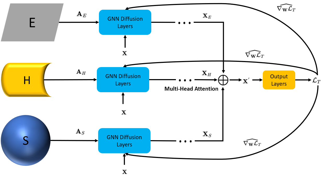
Combining Feature Representations from Candidate Latent Graphs using Attention. The optimal embedding space for latent graph inference is unknown and varies from task to task. Different embedding spaces come with distinct metrics, resulting in varying latent graphs. Instead of choosing an embedding space in advance, we aim to empower our model to select the best embedding space in a differentiable manner. To achieve this, we will not work with a single dDGM module for latent graph inference but rather employ multiple of them simultaneously. Each dDGM will utilize a different embedding space, suggesting a distinct candidate latent graph. Consequently, this approach will generate different downstream features as information from the upstream layer diffuses through each unique latent graph. Let us denote by the node feature representations obtained based on different embedding space manifolds , where is the number of nodes in the graph and the dimensionality of the node features. Next, we define as the collection of potential embedding space manifolds for each dDGM with cardinality . Additionally, consider to represent the row (or node) of the matrix . We calculate attention in the following manner:
| (1) |
In this equation, and represent the query and key weight matrices. Essentially, this equation enables the comparison of node feature representations for a specific node in the graph across various embedding spaces. The weight for the representation of the node within latent space , denoted as , is determined by averaging over all latent spaces:
| (2) |
The coefficient can be interpreted as the mean importance of manifold relative to other manifolds for the node representation. Finally, the overall combined node representation for the node, can be calculated via the weighted sum:
| (3) |
Once this is calculated, the resultant combined node feature matrix can be fed into the subsequent downstream GNN layers.
Attention-based Gradient Descent for Automatic Latent Space Selection. Although the attentional combination of feature representations discussed earlier provides valuable insights into selecting latent spaces, relying solely on these weights as straightforward indicators can be problematic if the GNN diffusion layers are not initialized carefully. Several factors, including variations in the initialization and training states of the GNN diffusion layers for each latent space , can serve as confounding variables that impact the allocation of attention weights to these spaces. To ensure an equitable assessment of different latent spaces throughout the training process, it is crucial to maintain consistent parameters for all the GNN diffusion layers that operate downstream of the parallel dDGM modules. In mathematical terms, our objective is to retain for all latent spaces in each training step. This effectively means we assess multiple candidate latent graphs simultaneously during the training of a single GNN, avoiding the need for an ensemble approach. As a result, we can identify the optimal candidate geometry for our model.
The initial step involves ensuring identical parameter initialization for each diffusion layer downstream of every dDGM module. It is important to note that multiple diffusion layers need to be initialized to maintain the integrity of the computational graph. However, in essence, we are evaluating the performance of various candidate latent graphs in parallel on a single model. During each training step, we substitute the initial gradients of the GNN parameters for each latent space, which are obtained through backpropagation, with an attention-based weighted gradient formed by combining individual gradients. We can define as the set of model parameters responsible for processing the latent graph generated from the embedding space . Let represent the gradient of the loss concerning these parameters for the downstream task. The attention weights for each , utilized to combine , are calculated by averaging the node attention weights , which are computed during the forward pass in line with Equation 2: where is the number of nodes. Finally, the attention-weighted gradient shared across all latent spaces is computed as follows:
| (4) |
This gradient can be employed to update all the parallel diffusion layers using any Stochastic Gradient Descent (SGD)-based optimization method, while ensuring uniform downstream GNN parameters across all latent spaces throughout the training process. The attention-based feature combination and gradient descent scheme together form our AMES latent space selection framework for embedding space selection.
Further Details on dDGM training. When training GNN models that incorporate dDGM latent graph inference modules, there are two distinct losses to consider. The first one, denoted as , assesses the model’s performance on downstream tasks, employing cross-entropy loss for classification and mean squared error (MSE) for regression, among other possibilities. Given that the GNN diffuses information using the latent graphs generated by the latent graph inference module, it is important to note that this loss exclusively updates the GNN parameters and does not propagate gradients through the dDGM. Hence, an additional loss term to update the internal learnable parameters of the dDGM is required, which is known as the graph loss, . This loss is based on the negative log likelihood of the probability that an edge exists between two nodes: The term is characterized as the disparity between two aspects: the average accuracy observed for the node and the correctness of the current prediction for that node’s label, represented as . Here, equals 1 if and 0 otherwise, where is the label prediction and the ground truth label. For regression tasks, the R2 score could be used in place of accuracy. In turn, the probability of an edge existing between two given nodes can be expressed as follows, where is a temperature parameter, is the geodesic distance function for a given embedding space manifold , and are the node feature representations of nodes and in layer , and signifies that the node features are passed through a parametrized function and later projected using the exponential map onto the corresponding manifold . For our attention-based model, the overall graph loss can be computed by simply adding up individual graph losses from each dDGM module:
| (5) |
It is worth noting that while latent graph inference could theoretically be applied to all layers of the GNN, practical experiments, as demonstrated in Kazi et al. (2022) and Sáez de Ocáriz Borde et al. (2023c), reveal that stacking multiple dDGM modules does not yield performance improvements, especially when considering the computational cost involved. Consequently, in our work, we will exclusively employ a single dDGM module for all experiments. During the training of AMES, we optimize both and using the Adam optimizer (Kingma and Ba, 2014). To ensure a fair comparison with prior work, we adopt the same number of training epochs and GNN parameterizations as in Sáez de Ocáriz Borde et al. (2023c). Specific details regarding the learning rate and weight decay can be found in Appendix A.1. For additional model architecture details refer to Appendix A.2, A.3 and A.4.
4 Training Interpretability Framework
In addition to numerical outcomes, we employ a gradient-based attribution approach, drawing inspiration from Simonyan et al. (2013), to assess the significance of each latent space’s influence on the downstream tasks. This serves as an interpretability analysis. The saliency maps suggested in Simonyan et al. (2013) are generated by calculating the gradient of the score function of the label class of an input image with respect to the pixels of the input image itself. In an intuitive sense, the gradient of a predicted label in relation to an input image measures how the model’s prediction changes when individual image pixels undergo slight modifications. Therefore, a larger gradient signifies a greater influence on the predictions. In our context, the score function is the cross-entropy loss for all the nodes in the graph. Hence, we take the gradient of the loss with respect to , the feature activations produced from individual latent graphs originating in distinct latent spaces, denoted as . This returns a gradient matrix since the loss is a scalar. Given that is high-dimensional and hard to visualize, we calculate its Frobenius norm:
| (6) |
which gives a scalar indicator of each latent space’s attribution to the node classification prediction and it is easier to track and visualize during training. During training initialization, all representations stemming from diverse latent embedding spaces are set to exert equal influence on the downstream representations, resulting in identical Frobenius norms. As training progresses, the attention coefficients begin to learn which latent graphs are more suitable for computation. By monitoring the Frobenius norm of the loss gradient, we can gauge the pace at which this adaptation occurs and identify which embedding spaces assume a dominant role in the learning process. We do notice the existence of other GNN interpretability approaches (Ying et al., 2019; Luo et al., 2020; Wang et al., 2021), however, these approaches mainly focusing on determining subgraphs that are important for individual predictions and hence are not suitable for our task.
5 Results
Experimental Setup and Numerical Evaluation. In this work, we focus on transductive node classification. We test AMES on five homophilic, heterophilic and real-world datasets. For each dataset, we perform 10-fold cross-validation where of the nodes are used for training and for testing in each split in line with Kazi et al. (2022). In this case, the task-specific loss is the cross-entropy loss. In our approach, we exclusively employ model spaces as candidate embedding spaces, which suffices to match the performance of prior methods that utilize product manifolds. It is worth noting that for homophilic graph benchmarks, we leverage the original dataset graph as an inductive bias. However, when dealing with heterophilic datasets, we have observed that starting from a point cloud yields more significant benefits. This preference arises from the fact that we perform diffusion with GCN layers. In the instance of TadPole, a real-world baseline dataset, we encounter a unique scenario where no initial input graph is available. Consequently, our latent graph inference system operates directly on the point cloud in this case. Table 1 displays the numerical results. AMES consistently demonstrates improved or comparable test set accuracy across various datasets compared to earlier models, even when those models employ more intricate embedding structures, such as product spaces. Notably, the H+S combination consistently surpasses all other models on nearly all five datasets. The key takeaway is that using our proposed model eliminates the need for random exploration among latent spaces.
| HOMOPHILIC DATASETS | HETEROPHILIC DATASETS | REAL-WORLD DATASETS | |||||
| Cora | CiteSeer | Chameleon | Squirrel | TadPole | |||
| Connections k | 7 | 5 | 2 | 3 | 3 | ||
| Baseline Models | |||||||
| dDGM-E | |||||||
| dDGM-H | |||||||
| dDGM-S | |||||||
| dDGM-ES | |||||||
| dDGM-EH | |||||||
| dDGM-HS | |||||||
| dDGM-EHH | |||||||
| dDGM-EHS | |||||||
| MLP | |||||||
| GCN | N/A | ||||||
| New Models (AMES) | |||||||
| AMES-H+S | |||||||
| AMES-E+H+S | |||||||
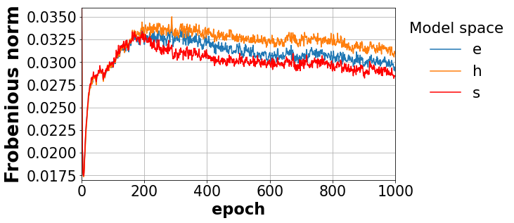
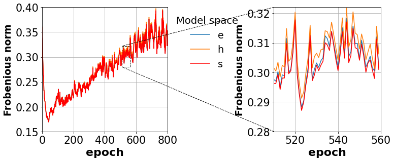
Interpretability Results. We create visualizations to track the average norm evolution across the 10 training folds. In the interest of conducting the interpretability analysis, despite the superior performance of H+S in principle, Figure LABEL:fig:e_h_s_no_inductive_bias_grad presents plots illustrating the average Frobenius norm of loss gradients for E+H+S. This allows us to monitor the learning progress across all model spaces, as opposed to focusing solely on two of them. The trends align with the data presented in Table 1 for all five datasets. In the case of Cora, it is noteworthy that appears to contribute the most, while makes the smallest contribution. For CiteSeer, although the gap between and is not as pronounced, both curves conform to the baseline results for single model spaces found in Table 1. For the heterophilic datasets we observe a similar trend, the models using hyperbolic space are superior and our framework learns to select the graph stemming from hyperbolic space as the main contributor, see Figure 2 and 2. In summary, our model demonstrates its ability to autonomously identify the embedding spaces that align most favorably with the baseline results. The attention weights assigned to each latent space closely correspond to their counterparts based on single model spaces in the baselines. As a result, our AMES effectively assesses the relative importance of the involved latent spaces based on their impact on downstream tasks. Furthermore, it becomes evident that the hyperbolic space consistently emerges as the preferred choice across the majority of the benchmark graph datasets we have employed. This intriguing finding may merit further investigation beyond the scope of this study and seems to align with the common belief that hyperbolic space is better suited for encoding latent tree structures (Kratsios et al., 2023), such as those present in our graph benchmarks.
fig:e_h_s_no_inductive_bias_grad
\subfigure[Cora]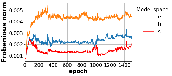 \subfigure[CiteSeer]
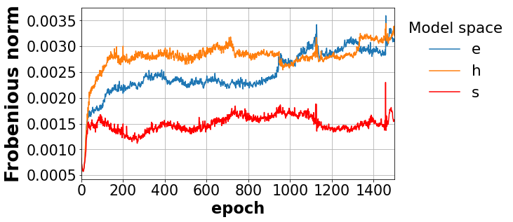 \subfigure[Squirrel]
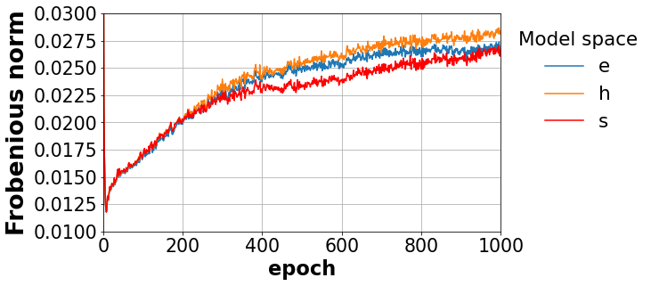 \subfigure[Chameleon]
 \subfigure[TadPole]
6 Conclusion
In this work we have introduced AMES, a fully-differentiable mechanism designed for embedding space selection within the context of latent graph inference. In contrast to prior methods, our approach circumvents the need for conducting random searches across the combinatorial spectrum of potential product manifold combinations. Instead, it possesses the capacity to dynamically learn the optimal embedding space through a single model. Moreover, we offer interpretability techniques to monitor this learning process. Notably, our method maintains performance levels on par with other models in the existing literature, all while alleviating the computational burden associated with conducting multiple experiments in pursuit of the ideal embedding space.
Future Work. Our model selection remains grounded in constant curvature model spaces, implying that local curvature control remains a challenge. While the application of attention could potentially yield more flexible representations than what constant curvature model spaces can offer on their own, additional research is required to gain a deeper understanding of how this approach influences the curvature of the embedding space. Note that since the method does not distinctly select a candidate embedding space but rather combines model spaces using attention, the model is effectively learning a new metric.
References
- Alon and Yahav (2021) Uri Alon and Eran Yahav. On the bottleneck of graph neural networks and its practical implications. In International Conference on Learning Representations, 2021. URL https://openreview.net/forum?id=i80OPhOCVH2.
- Bahdanau et al. (2014) Dzmitry Bahdanau, Kyunghyun Cho, and Yoshua Bengio. Neural machine translation by jointly learning to align and translate. CoRR, abs/1409.0473, 2014. URL https://api.semanticscholar.org/CorpusID:11212020.
- Bronstein et al. (2021) Michael M Bronstein, Joan Bruna, Taco Cohen, and Petar Veličković. Geometric deep learning: Grids, groups, graphs, geodesics, and gauges. arXiv preprint arXiv:2104.13478, 2021.
- Chamberlain et al. (2021) Ben Chamberlain, James Rowbottom, Maria I Gorinova, Michael Bronstein, Stefan Webb, and Emanuele Rossi. Grand: Graph neural diffusion. In International Conference on Machine Learning, pages 1407–1418. PMLR, 2021.
- Chami et al. (2019) Ines Chami, Zhitao Ying, Christopher Ré, and Jure Leskovec. Hyperbolic graph convolutional neural networks. Advances in neural information processing systems, 32, 2019.
- Chen et al. (2020) Yu Chen, Lingfei Wu, and Mohammed Zaki. Iterative deep graph learning for graph neural networks: Better and robust node embeddings. Advances in neural information processing systems, 33:19314–19326, 2020.
- Cosmo et al. (2020) Luca Cosmo, Anees Kazi, Seyed-Ahmad Ahmadi, Nassir Navab, and Michael Bronstein. Latent-graph learning for disease prediction. In Medical Image Computing and Computer Assisted Intervention–MICCAI 2020: 23rd International Conference, Lima, Peru, October 4–8, 2020, Proceedings, Part II 23, pages 643–653. Springer, 2020.
- De Bortoli et al. (2022) Valentin De Bortoli, Emile Mathieu, Michael Hutchinson, James Thornton, Yee Whye Teh, and Arnaud Doucet. Riemannian score-based generative modelling. Advances in Neural Information Processing Systems, 35:2406–2422, 2022.
- Deac et al. (2022) Andreea Deac, Marc Lackenby, and Petar Velivckovi’c. Expander graph propagation. In LOG IN, 2022.
- Franceschi et al. (2019) Luca Franceschi, Mathias Niepert, Massimiliano Pontil, and Xiao He. Learning discrete structures for graph neural networks. In International conference on machine learning, pages 1972–1982. PMLR, 2019.
- Gasteiger et al. (2019) Johannes Gasteiger, Stefan Weißenberger, and Stephan Günnemann. Diffusion improves graph learning. Advances in neural information processing systems, 32, 2019.
- Hensel et al. (2021) Felix Hensel, Michael Moor, and Bastian Rieck. A survey of topological machine learning methods. Frontiers in Artificial Intelligence, 4:681108, 2021.
- Huang et al. (2022) Chin-Wei Huang, Milad Aghajohari, Joey Bose, Prakash Panangaden, and Aaron C Courville. Riemannian diffusion models. Advances in Neural Information Processing Systems, 35:2750–2761, 2022.
- Jin et al. (2020) Wei Jin, Yao Ma, Xiaorui Liu, Xianfeng Tang, Suhang Wang, and Jiliang Tang. Graph structure learning for robust graph neural networks. In Proceedings of the 26th ACM SIGKDD international conference on knowledge discovery & data mining, pages 66–74, 2020.
- Kazi et al. (2022) Anees Kazi, Luca Cosmo, Seyed-Ahmad Ahmadi, Nassir Navab, and Michael M Bronstein. Differentiable graph module (dgm) for graph convolutional networks. IEEE Transactions on Pattern Analysis and Machine Intelligence, 45(2):1606–1617, 2022.
- Kingma and Ba (2014) Diederik P Kingma and Jimmy Ba. Adam: A method for stochastic optimization. arXiv preprint arXiv:1412.6980, 2014.
- Kratsios et al. (2023) Anastasis Kratsios, Ruiyang Hong, and Haitz Sáez de Ocáriz Borde. Capacity bounds for hyperbolic neural network representations of latent tree structures, 2023.
- Luo et al. (2020) Dongsheng Luo, Wei Cheng, Dongkuan Xu, Wenchao Yu, Bo Zong, Haifeng Chen, and Xiang Zhang. Parameterized explainer for graph neural network. Advances in neural information processing systems, 33:19620–19631, 2020.
- Mathieu et al. (2019) Emile Mathieu, Charline Le Lan, Chris J Maddison, Ryota Tomioka, and Yee Whye Teh. Continuous hierarchical representations with poincaré variational auto-encoders. Advances in neural information processing systems, 32, 2019.
- Mettes et al. (2019) Pascal Mettes, Elise Van der Pol, and Cees Snoek. Hyperspherical prototype networks. Advances in neural information processing systems, 32, 2019.
- Sáez de Ocáriz Borde et al. (2023a) Haitz Sáez de Ocáriz Borde, Alvaro Arroyo, Ismael Morales, Ingmar Posner, and Xiaowen Dong. Neural latent geometry search: Product manifold inference via gromov-hausdorff-informed bayesian optimization, 2023a.
- Sáez de Ocáriz Borde et al. (2023b) Haitz Sáez de Ocáriz Borde, Alvaro Arroyo, and Ingmar Posner. Projections of model spaces for latent graph inference. In ICLR 2023 Workshop on Physics for Machine Learning, 2023b.
- Sáez de Ocáriz Borde et al. (2023c) Haitz Sáez de Ocáriz Borde, Anees Kazi, Federico Barbero, and Pietro Lio. Latent graph inference using product manifolds. The Eleventh International Conference on Learning Representations, 2023c.
- Simonyan et al. (2013) Karen Simonyan, Andrea Vedaldi, and Andrew Zisserman. Deep inside convolutional networks: Visualising image classification models and saliency maps. arXiv preprint arXiv:1312.6034, 2013.
- Vaswani et al. (2017) Ashish Vaswani, Noam Shazeer, Niki Parmar, Jakob Uszkoreit, Llion Jones, Aidan N Gomez, Łukasz Kaiser, and Illia Polosukhin. Attention is all you need. Advances in neural information processing systems, 30, 2017.
- Wang et al. (2021) Xiang Wang, Yingxin Wu, An Zhang, Xiangnan He, and Tat seng Chua. Causal screening to interpret graph neural networks, 2021. URL https://openreview.net/forum?id=nzKv5vxZfge.
- Wang et al. (2019) Yue Wang, Yongbin Sun, Ziwei Liu, Sanjay E Sarma, Michael M Bronstein, and Justin M Solomon. Dynamic graph cnn for learning on point clouds. Acm Transactions On Graphics (tog), 38(5):1–12, 2019.
- Ying et al. (2019) Zhitao Ying, Dylan Bourgeois, Jiaxuan You, Marinka Zitnik, and Jure Leskovec. Gnnexplainer: Generating explanations for graph neural networks. Advances in neural information processing systems, 32, 2019.
- Zhu et al. (2021) Yanqiao Zhu, Weizhi Xu, Jinghao Zhang, Qiang Liu, Shu Wu, and Liang Wang. Deep graph structure learning for robust representations: A survey. arXiv preprint arXiv:2103.03036, 14, 2021.
Appendix A Training Statistics and Model Architecture
This section provides the training statistics and model architectures for both the dDGM and the downstream GNN diffusion layer applied to homophilic, heterophilic, and real-world datasets. In general, we closely follow the model architecture and training statistics outlined in Sáez de Ocáriz Borde et al. (2023c), with only minor differences.
A.1 Training Statistics
| Training Epochs | Learning Rate | Weight Decay | |
|---|---|---|---|
| Cora | 1,500 | ||
| CiteSeer | 1,500 | ||
| Squirrel | 1,000 | ||
| Chameleon | 1,000 | ||
| TadPole | 800 |
| Training Epochs | Learning Rate | Weight Decay | |
|---|---|---|---|
| Cora | 1,500 | ||
| CiteSeer | 1,500 | ||
| Squirrel | 1,000 | ||
| Chameleon | 1,000 | ||
| TadPole | 800 |
A.2 Model Architecture for Homophilic Datasets
| Layer size | dDGM | |
|---|---|---|
| (No. features, 32) | Linear | |
| N/A | ELU | |
| (32, 16 per model space) | GCN Conv | |
| N/A | ELU | |
| (16 per model space, 4 per model space) | GCN Conv | |
| N/A | Sigmoid |
| Layer size | MLP | GCN | GCN-dDGM | |
|---|---|---|---|---|
| N/A | N/A | dDGM | ||
| (No. features, 32) | Linear | GCN Conv | GCN Conv | |
| N/A | ELU | ELU | ELU | |
| (32, 16) | Linear | GCN Conv | GCN Conv | |
| N/A | ELU | ELU | ELU | |
| (16, 8) | Linear | GCN Conv | GCN Conv | |
| N/A | ELU | ELU | ELU | |
| (8, 8) | Linear | Linear | Linear | |
| N/A | ELU | ELU | ELU | |
| (8, 8) | Linear | Linear | Linear | |
| N/A | ELU | ELU | ELU | |
| (8, No.classes) | Linear | Linear | Linear |
A.3 Model Architecture for Heterophilic Datasets
| Layer size | dDGM | |
|---|---|---|
| (No. features, 32) | Linear | |
| N/A | BatchNorm | |
| N/A | ELU | |
| (32, 4 per model space) | Linear | |
| N/A | BatchNorm | |
| N/A | ELU | |
| (4 per model space, 4 per model space) | Linear | |
| N/A | BatchNorm | |
| N/A | Sigmoid |
| Layer size | MLP | GCN-dDGM | |
|---|---|---|---|
| N/A | dDGM | ||
| (No. features, 16) | Linear | GCN Conv | |
| N/A | ELU | ELU | |
| (16, 8) | Linear | GCN Conv | |
| N/A | ELU | ELU | |
| (8, 8) | Linear | Linear | |
| N/A | BatchNorm | BatchNorm | |
| N/A | ELU | ELU | |
| (8, No.classes) | Linear | Linear |
A.4 Model Architecture for TadPole
| Layer size | dDGM | |
|---|---|---|
| (No. features, 16 per model space) | Linear | |
| N/A | BatchNorm | |
| N/A | ELU | |
| (16 per model space, 4 per model space) | Linear | |
| N/A | BatchNorm | |
| N/A | Sigmoid |
| Layer size | MLP | GCN-dDGM | |
|---|---|---|---|
| N/A | dDGM | ||
| (No. features, 32) | Linear | GCN Conv | |
| N/A | ELU | ELU | |
| (32, 16) | Linear | GCN Conv | |
| N/A | ELU | ELU | |
| (16, 8) | Linear | GCN Conv | |
| N/A | ELU | ELU | |
| (8, 8) | Linear | Linear | |
| N/A | BatchNorm | BatchNorm | |
| N/A | ELU | ELU | |
| (8, 8) | Linear | Linear | |
| N/A | BatchNorm | BatchNorm | |
| N/A | ELU | ELU | |
| (8, No.classes) | Linear | Linear |