Entangled View-Epipolar Information Aggregation for
Generalizable Neural Radiance Fields

Abstract

Generalizable NeRF can directly synthesize novel views across new scenes, eliminating the need for scene-specific re-training in vanilla NeRF. A critical enabling factor in these approaches is the extraction of a generalizable 3D representation by aggregating source-view features. In this paper, we propose an Entangled View-Epipolar Information Aggregation method dubbed EVE-NeRF. Different from existing methods that consider cross-view and along-epipolar information independently, EVE-NeRF conducts the view-epipolar feature aggregation in an entangled manner by injecting the scene-invariant appearance continuity and geometry consistency priors to the aggregation process. Our approach effectively mitigates the potential lack of inherent geometric and appearance constraint resulting from one-dimensional interactions, thus further boosting the 3D representation generalizablity. EVE-NeRF attains state-of-the-art performance across various evaluation scenarios. Extensive experiments demonstate that, compared to prevailing single-dimensional aggregation, the entangled network excels in the accuracy of 3D scene geometry and appearance reconstruction. Our project page is https://github.com/tatakai1/EVENeRF.

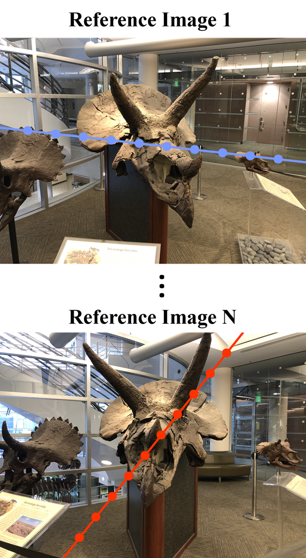
(a) Source views

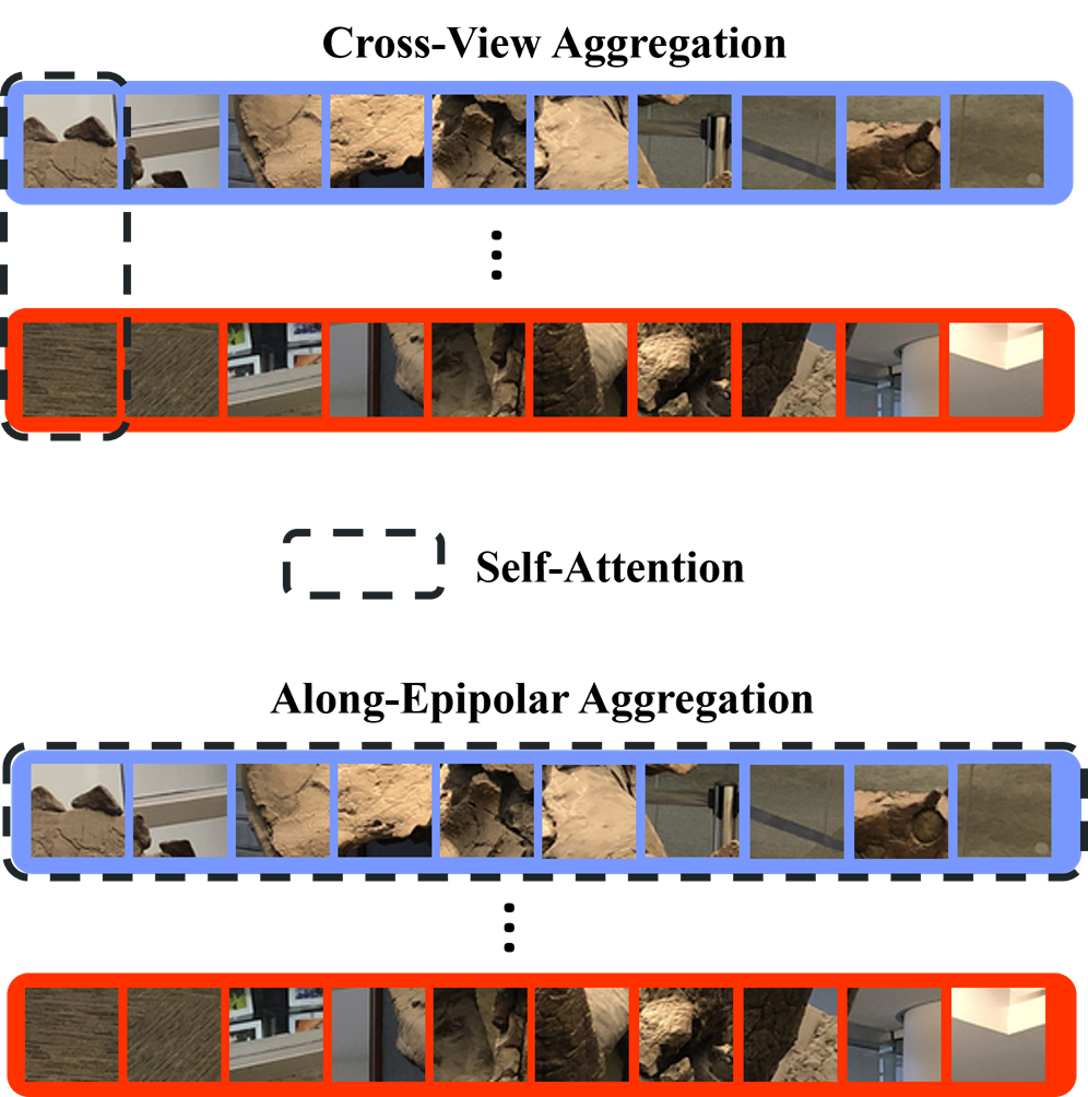
(b) Two ways of generalizable information aggregation

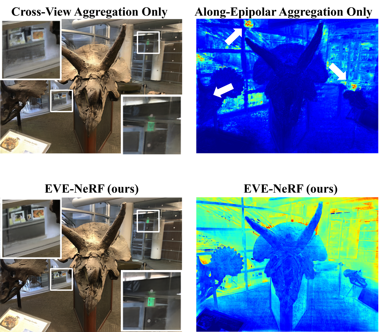
(c) Generalizable novel view synthesis

Figure 1: Given the sampling points along a target ray that are re-projected on the epipolar lines in each source view (a), existing approaches [32, 38] employ attention mechanism to aggregate the cross-view features for each sampling point and perform epipolar aggregation of sampling points along the epipolar lines within individual views (b), either sequentially or circularly. However, our investigation reveals the limitations in existing strategies: exclusively aggregating cross-view information results in rendering artifacts, stemming from the absence of appearance continuity between adjacent depth provided by epipolar cues. Conversely, relying solely on epipolar information leads to depth map discontinuities due to the absence of geometry consistency across multiple views. Our proposed EVE-NeRF harnesses both cross-view and along-epipolar information in an entangled manner and effectively addresses the above issues (c).

1 Introduction

The neural radiance fields (NeRF) [25], along with its subsequent refinements [1, 47, 2], has demonstrated remarkable efficacy in the realm of novel view synthesis. Despite these advancements, the methods along this vein often pertain to the training scene thus necessitating re-training for synthesizing new scenes. Such drawbacks severely constrain their practical applications.

More recently, the development of generalizable NeRF models [48, 41, 4] has emerged as a promising solution to address this challenge. These models can directly synthesize novel views across new scenes, eliminating the need for scene-specific re-training. A critical enabling factor in these approaches is the synthesis of a generalizable 3D representation by aggregating source-view features. Instead of densely aggregating every pixel in the source images, prior works draw inspiration from the epipolar geometric constraint across multiple views to aggregate view or epipolar information [19, 29, 38, 32, 40]. To capitalize on cross-view prior, specific methodologies [38, 19] interact with the re-projected feature information in the reference view at a predefined depth. On the along-epipolar aspect [32, 33], some methods employ self-attention mechanisms to sequentially obtain the entire epipolar line features in each reference view.

We posit that both view and epipolar aggregation are crucial for learning a generalizable 3D representation: cross-view feature aggregation is pivotal to capturing geometric information, as the features from different views that match tend to be on the surface of objects. Concurrently, epipolar feature aggregation contributes by extracting depth-relevant appearance features from the reference views associated with the target ray, thus achieving a more continuous appearance representation. Nevertheless, the prevailing methods often execute view and epipolar aggregation independently [38, 19] or in a sequential manner [32], thereby overlooking the simultaneous interaction of appearance and geometry information.

In this paper, we introduce a novel Entangled View-Epipolar information aggregation network, denoted as EVE-NeRF. EVE-NeRF is designed to enhance the quality of generalizable 3D representation through the simultaneous utilization of complementary appearance and geometry information. The pivotal components of EVE-NeRF are the View-Epipolar Interaction Module (VEI) and the Epipolar-View Interaction Module (EVI). Both modules adopt a dual-branch structure to concurrently integrate view and epipolar information. On one hand, VEI comprises a view transformer in its first branch to engage with the features of sampling points re-projected on all source views. In the second branch, VEI is equipped with an Along-Epipolar Perception submodule to inject the appearance continuity prior to the view aggregation results. On the other hand, EVI consists of an epipolar transformer in its first branch to aggregate features from sampling points along the entire epipolar line in each source view. In the second branch, EVI utilizes a Multi-View Calibration submodule to incorporate the geometry consistency prior to the epipolar aggregation representation. The alternating organization of EVI and VEI results in a generalizable condition for predicting the color of target rays based on NeRF volumetric rendering.

Compared to the prevailing methods such as GNT [38] and GPNR [32], EVE-NeRF distinguishes itself in its ability to synthesize a target ray by entangling epipolar and view information. This capability serves to offset the appearance and geometry prior losses that typically arises from single-dimensional aggregation operations (see Figure 1). Our main contributions can be summarized as follows:

• Through extensive investigation, we have revealed the under-explored issues of prevailing cross-view and along-epipolar information aggregation methods for generalizable NeRF.

• We propose EVE-NeRF, which harnesses the along-epipolar and cross-view information in an entangled manner. EVE-NeRF complements the cross-view aggregation with appearance continuity prior and calibrates the along-epipolar aggregation with geometry consistency prior.

• EVE-NeRF produces more realistic novel-perspective images and depth maps for previously unseen scenes without any additional ground-truth 3D data. Experiments demonstrate that EVE-NeRF achieves state-of-the-art performance in various novel scene synthesis tasks.

2 Related Work

NeRF and Generalizable NeRF.  Recently, NeRF [25] has made groundbreaking advancements in the field of novel view synthesis through a compact implicit representation based on differentiable rendering. Subsequent developments in the NeRF framework have explored various avenues, enhancing rendering quality [49, 1, 2, 16, 3], accelerating rendering speed [47, 15, 34, 5, 28, 8], applicability to both rigid and non-rigid dynamic scenes [26, 27, 37, 36, 14, 50], and extending its capabilities for editing [22, 39, 35, 45, 44].

The original NeRF and its subsequent improvements have achieved successful performance but suffered from the limitation of being trainable and renderable only in a single scene, which restricts their practical applications. One solution to this issue is conditioning on CNN features from the known view images, which align with the input coordinates of NeRF. PixelNeRF [48] encodes input images into pixel-aligned feature grids, combining image features with corresponding spatial positions and view directions in a shared MLP to output colors and densities. MVSNeRF [4] utilizes a cost volume to model the scene, with interpolated features on volume conditioned. Our approach also employs CNN features from known views, and we input the processed, pixel-aligned features into NeRF’s MLP network to predict colors and densities. However, unlike PixelNeRF and similar methods [48, 4, 7], which use average pooling for handling multiple views, our approach learns multi-view information and assigns weights to each view based on its relevance.

Generalizable NeRF with Transformers.  More recently, generalizable novel view synthesis methods [41, 32, 20, 40, 10, 21, 29, 17, 11] have incorporated transformer-based networks to enhance visual features from known views. These approaches employ self-attention or cross-attention mechanisms along various dimensions such as depth, view, or epipolar, enabling high-quality feature interaction and aggregation. GeoNeRF [19] concatenates view-independent tokens with view-dependent tokens and feeds them into a cross-view aggregation transformer network to enhance the features of the cost volume. GPNR [32] employs a 3-stage transformer-based aggregation network that sequentially interacts with view, epipolar, and view information. GNT [38] and its subsequent work, GNT-MOVE [11], utilize a 2-stage transformer-based aggregation network, first performing cross-view aggregation and then engaging depth information interaction. ContraNeRF [46] initially employs a two-stage transformer-based network for geometry-aware feature extraction, followed by the computation of positive and negative sample contrastive loss based on ground-truth depth values.

Inspired by these developments, we have analyzed the limitations of single-dimensional aggregation transformer networks and introduced EVE-NeRF that achieves efficient interaction between the complementary appearance and geometry information across different dimensions. Moreover, our method does not require any ground-truth depth information for model training.

3 Problem Formulation

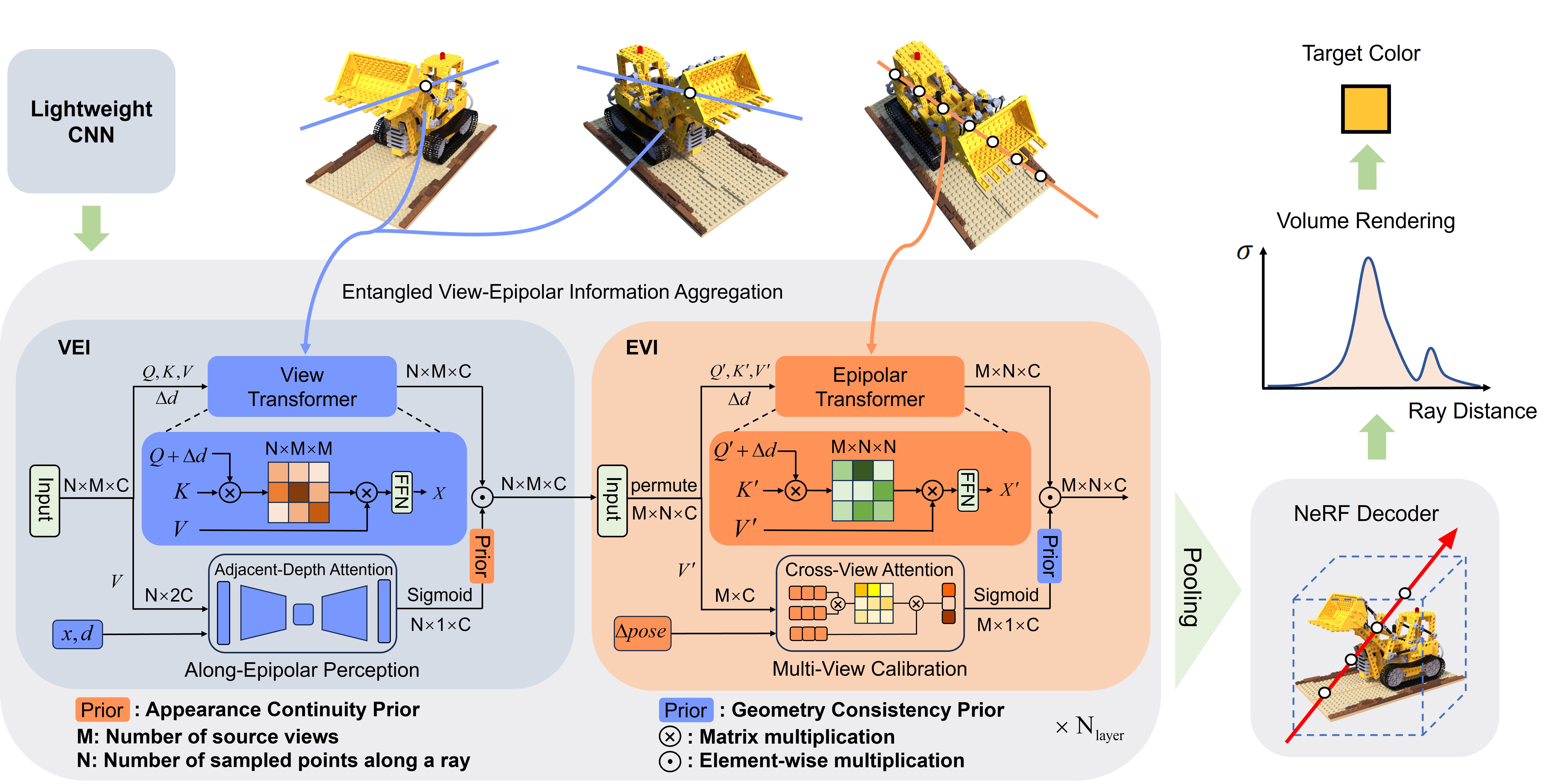
Figure 2: Pipline of EVE-NeRF. 1) We first employ a lightweight CNN to extract features of the epipolar sampling points from source views. 2) Through the Entangled View-Epipolar Information Aggregation, we complementarily enable information interaction in both the view and epipolar dimensions to produce generalizable multi-view epipolar features. 3) We use the NeRF Decoder to obtain color and density for the sampling points and predict the target color based on volume rendering.

Our objective is to train a generalizable NeRF capable of comprehending 3D information from scenes the model has never encountered before and rendering new perspective images. Specifically, given $N$ source images for a particular scene $\boldsymbol{I}=\{\boldsymbol{I}_{i}\}_{i=1}^{N}$ and their corresponding camera intrinsic and extrinsic parameters $\boldsymbol{K}=\{\boldsymbol{K}_{i}\}_{i=1}^{N},\boldsymbol{P}=\{\boldsymbol{P}_{i}=[\boldsymbol{R}_{i},\boldsymbol{t}_{i}]\}_{i=1}^{N}$, most generalizable NeRF methods [48, 41, 4] can be formulated with a generalizable feature extraction network $\mathcal{F}_{\theta}$ and a rendering network $\mathcal{G}_{\phi}$:

$$\mathcal{F}_{\theta}:(\boldsymbol{I},\boldsymbol{K},\boldsymbol{P})\rightarrow\boldsymbol{z},\quad\mathcal{G}_{\phi}:(\boldsymbol{x},\boldsymbol{d},\boldsymbol{z})\rightarrow(\boldsymbol{c},\sigma),$$ (1)

where $\boldsymbol{x}$ and $\boldsymbol{d}$ represent the 3D point position and the direction of the target ray’s sampling points, while $\boldsymbol{c}$ and $\sigma$ are the predicted color and density, respectively. Similar to vanilla NeRF, $\boldsymbol{c}$ and $\sigma$ are utilized to compute the final color value of the target ray through volume rendering. The variable $\boldsymbol{z}$ represents generalizable 3D representation of the scene provided by the feature extraction network. $\Theta$ and $\phi$ denote the learnable parameters of the networks.

4 Methodology

Overview.  Figure 2 provides an overview of EVE-NeRF, which includes a lightweight CNN-based image feature extractor, two dual-branch transformer-based modules named View-Epipolar Interaction (VEI) and Epipolar-View Interaction (EVI), respectively, and a conditioned NeRF decoder. Source images are first forwarded to a lightweight CNN and are transferred to feature maps. In the following, VEI and EVI are alternatively organized to aggregate the view-epipolar features in an entangled manner. The inter-branch information interaction mechanism within VEI and EVI capitalizes on the scene-invariant geometry and appearance priors to further calibrate the aggregated features. The output of the Entangle View-Epipolar Information Aggregation is a generalizable 3D representation $\boldsymbol{z}$. Finally, a conditioned NeRF decoder is employed for predicting the color and density values of the target ray based on $\boldsymbol{z}$ for volume rendering.

5 Lightweight CNN

For $M$ source views input $\{\boldsymbol{I}_{i}\}_{i=1}^{M}$, we first extract convolutional features $\{\boldsymbol{F}_{i}^{c}\}_{i=1}^{M}$ for each view independently using a lightweight CNN with sharing weights (see Appendix A.4). Unlike previous generalizable NeRF methods [4, 38] that employ deep convolutional networks like U-Net [30], we use this approach since convolutional features with large receptive fields may not be advantageous for extracting scene-generalizable features. Additionally, features derived from the re-projected sampling points guided by epipolar geometry are more focused on local information.

5.1 View-Epipolar Interaction

The View-Epipolar Interaction Module (VEI) is designed as a dual-branch structure, with one branch comprising the View Transformer and the other the Along-Epipolar Perception. The VEI input $\boldsymbol{X}\in\mathbb{R}^{N\times M\times C}$ comes from the CNN feature map interpolated features or from the output of the previous layer of EVI, and the VEI output $\boldsymbol{Y_{VEI}}$ is used as the input to the current layer of EVI.

View Transformer.  The View Transformer is responsible for aggregating features across view dimensions. The view transformer takes the input $\boldsymbol{X}$, allowing it to perform self-attention operations in the view dimension ($M$). To be more specific, the query, key, and value matrices are computed using linear mappings:

$$\boldsymbol{Q}=\boldsymbol{X}\boldsymbol{W_{Q}},\,\boldsymbol{K}=\boldsymbol{X}\boldsymbol{W_{K}},\,\boldsymbol{V}=\boldsymbol{X}\boldsymbol{W_{V}},$$ (2)

where $\boldsymbol{W_{Q}},\boldsymbol{W_{K}},\boldsymbol{W_{V}}\in\mathbb{R}^{C\times C}$ are the linear mappings without biases. These matrices are then split into $h$ heads $\boldsymbol{Q}=[\boldsymbol{Q}^{1},\cdots,\boldsymbol{Q}^{h}]$, $\boldsymbol{K}=[\boldsymbol{K}^{1},\cdots,\boldsymbol{K}^{h}]$, and $\boldsymbol{V}=[\boldsymbol{V}^{1},\cdots,\boldsymbol{V}^{h}]$, each with $d=C/h$ channels. To enable the model to learn the relative spatial relationships between the target view and the source views, we integrate the differences $\Delta\boldsymbol{d}^{s}$ (see Appendix A.2) between the target view and the source views into the self-attention mechanism:

$$\boldsymbol{\tilde{X}}^{i}=\text{softmax}\left(\left(\boldsymbol{Q}^{i}+\Delta\boldsymbol{d}^{s}\right)\left(\boldsymbol{K^{i}}\right)^{\top}\right)\boldsymbol{V}^{i}.$$ (3)

Ultimately, we obtain $\boldsymbol{\tilde{X}}=[\boldsymbol{\tilde{X}}^{i},\cdots,\boldsymbol{\tilde{X}}^{h}]$, and we employ a conventional Feed-Forward Network (FFN) to perform point-wise feature transformation:

$$\boldsymbol{Y}=\text{FFN}(\boldsymbol{\tilde{X}})+\boldsymbol{\tilde{X}}.$$ (4)

Along-Epipolar Perception.  The Along-Epipolar Perception, serving as the second branch of VEI, aims to extract view-independent depth information to provide appearance continuity prior to the 3D representation. We compute the mean and variance of $\boldsymbol{V}\in\mathbb{R}^{N\times M\times C}$ in the view dimension ($M$) within the view transformer to obtain the global view-independent feature $\boldsymbol{f}^{0}\in\mathbb{R}^{N\times 2C}$. We proceed to perceive the depth information along the entire ray through an adjacent-depth attention (1D Convolution AE) in the ray dimension ($N$). Since the information along an epipolar line is inherently continuous, a convolution operation that is seen as a kind of adjacent attention can learn the appearance continuity prior, which predicts the importance weights $\operatorname{w}_{i}^{v}$ for the sampling points:

$$\boldsymbol{f}^{1}=\text{concat}\left(\boldsymbol{f}^{0},\boldsymbol{x},\boldsymbol{d}\right),$$

$$\{\operatorname{w}_{i}^{v}\}_{i=1}^{N}=\text{sigmoid}\left(\text{AE}\left(\{\boldsymbol{f}^{1}_{i}\}_{i=1}^{N}\right)\right),$$ (5)

where $\boldsymbol{x}$ and $\boldsymbol{d}$ refer to the 3D point position and the direction of the target ray’s sampling point. Particularly, $\boldsymbol{d}$ is copied to the same dimension as $\boldsymbol{x}$. GeoNeRF [19] also employs an AE network to predict coherent volume densities. However, our approach is more similar to an adjacent attention mechanism predicting depth importance weights and learning appearance continuity prior based on global epipolar features.

Combining the output of the View Transformer and Along-Epipolar Perception, the final output of VEI is calculated as follows:

$$\boldsymbol{Y_{VEI}}=\boldsymbol{w}^{v}\cdot\boldsymbol{Y},$$ (6)

where $\boldsymbol{w}^{v}=[\operatorname{w}_{1}^{v},\cdots,\operatorname{w}_{N}^{v}]$, $\boldsymbol{Y_{VEI}}$ denotes the VEI’s output, and $\cdot$ denotes element-wise multiplication.

5.2 Epipolar-View Interaction

Similar to VEI, The Epipolar-View Interaction Module (EVI) consists of two branches, the Epipolar Transformer and the Multi-View Calibration. The EVI input $\boldsymbol{X^{\prime}}\in\mathbb{R}^{M\times N\times C}$ comes from the output of the current layer of VEI, and the EVI output $\boldsymbol{Y_{EVI}}$ is used as the input to the next layer of EVIs or as the total output of the aggregation network.

Epipolar Transformer.  The Epipolar Transformer takes the input $\boldsymbol{X^{\prime}}$, enabling self-attention operations in the epipolar dimension ($N$). In particular, the epipolar transformer shares the same network structure as the view transformer above:

$$\boldsymbol{Q^{\prime}}=\boldsymbol{X^{\prime}}\boldsymbol{W^{\prime}_{Q}},\,\boldsymbol{K^{\prime}}=\boldsymbol{X^{\prime}}\boldsymbol{W^{\prime}_{K}},\,\boldsymbol{V^{\prime}}=\boldsymbol{X^{\prime}}\boldsymbol{W^{\prime}_{V}},$$

$$\boldsymbol{\tilde{X^{\prime}}}^{i}=\text{softmax}\left(\left(\boldsymbol{Q^{\prime}}^{i}+\Delta\boldsymbol{d^{\prime}}^{s}\right)\left(\boldsymbol{K^{\prime}}^{i}\right)^{\top}\right)\boldsymbol{V^{\prime}}^{i},$$

$$\boldsymbol{Y^{\prime}}=\text{FFN}(\boldsymbol{\tilde{X^{\prime}}})+\boldsymbol{\tilde{X^{\prime}}},$$ (7)

where $\boldsymbol{X}^{\prime}[i,j,k]=\boldsymbol{X}[j,i,k]$, $\boldsymbol{d^{\prime}}^{s}[i,j,k]=\boldsymbol{d}^{s}[j,i,k]$, $i,j,k$ denote the 1st ($M$), 2nd ($N$), and 3rd dimensions ($C$) respectively.

Multi-View Calibration.  The Multi-View Calibration, serving as the second branch of the EVI module, is employed to aggregate cross-view features and provide geometry consistency prior, aiming at calibrating the epipolar features. We calculate the weight values $\operatorname{w}_{j}^{e}$ for the target rays in each source view using the cross-view attention mechanism. In this process, we utilize $\boldsymbol{V}^{\prime}\in\mathbb{R}^{M\times N\times C}$ from the epipolar transformer as the input:

$$\boldsymbol{q}=\text{max}(\boldsymbol{V}^{\prime})+\text{linear}(\Delta\boldsymbol{pose}),$$

$$\{\operatorname{w}_{j}^{e}\}_{j=1}^{M}=\text{sigmoid}\left(\text{Self-Attn}\left(\boldsymbol{q},\boldsymbol{q},\boldsymbol{q}\right)\right),$$ (8)

where $\Delta\boldsymbol{pose}$ (see Appendix A.3) refers to the difference between the source view camera pose and the target view camera pose, and linear denotes the linear layer. Ultimately, incorporating the regression results of multi-view calibration, the output of the EVI is calculated as follows:

$$\boldsymbol{Y_{EVI}}=\boldsymbol{w}^{e}\cdot\boldsymbol{Y^{\prime}},$$ (9)

where $\boldsymbol{w}^{e}=[\operatorname{w}_{1}^{e},\cdots,\operatorname{w}_{M}^{e}]$, $\boldsymbol{Y_{EVI}}$ denotes the EVI’s output, and $\cdot$ denotes element-wise multiplication.

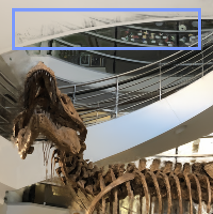
(a) only view transformer

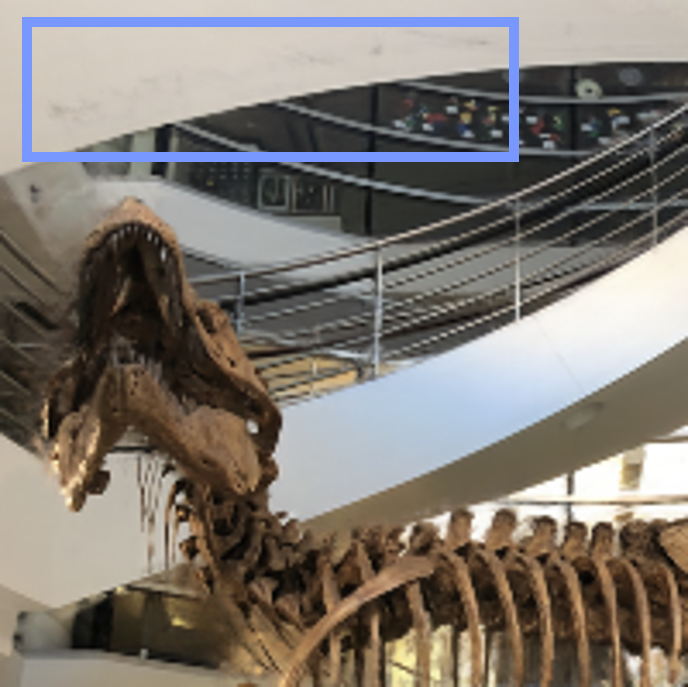
(b) w/ along-epipolar perception

(c) EVE-NeRF
(ours)

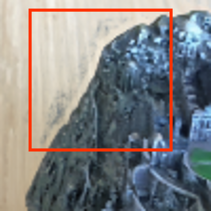
(d) only epipolar transformer

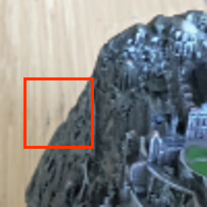
(e) w/ multi-view calibration

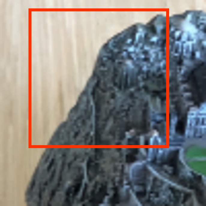
(f) EVE-NeRF
(ours)

Figure 3: The along-epipolar perception provides appearance continuity prior through adjacent-depth attention along the ray, while the multi-view calibration offers geometry consistency prior via cross-view attention. Our proposed method significantly reduces artifacts in rendering new views compared to single-dimension transformers.

5.3 Conditioned NeRF Decoder

We follow the established techniques of previous works [48] to construct an MLP-based rendering network. We also condition 3D points on a ray using the generalizable 3D representation $\boldsymbol{z}$ based-on Eq. 1. Nevertheless, we diverge from the traditional MLP decoder [25], which processes each point on a ray independently. Instead, we take a more advanced approach by introducing cross-point interactions. For this purpose, we employ the ray Transformer from IBRNet [41] in our implementation. After the rendering network predicts the emitted color $\boldsymbol{c}$ and volume density $\sigma$, we can generate target pixel color using volume rendering [25]:

$$\boldsymbol{C}=\sum_{i=1}^{N}T_{i}\left(1-\exp\left(-\sigma_{i}\delta_{i}\right)\right)\boldsymbol{c}_{i},\quad T_{i}=\exp(-\sum_{j}^{i-1}\sigma_{j}\delta_{j}),$$ (10)

where $\boldsymbol{c}_{i},\sigma_{i}$ which are calculated based on Eq. 1, refer to the color and density of the $i$-th sampling point on the ray.

5.4 Training Objectives

EVE-NeRF is trained solely using a photometric loss function, without the need for additional ground-truth 3D data. Specifically, our training loss function is as follows:

$$\mathcal{L}=\sum_{\boldsymbol{p}\in\mathcal{P}}\left\|\boldsymbol{C}_{pred}-\boldsymbol{C}_{gt}\right\|_{2}^{2},$$ (11)

where $\mathcal{P}$ represents a set of pixel points in a training batch, $\boldsymbol{C}_{pred},\boldsymbol{C}_{gt}$ respectively represent the rendering color for pixel $\boldsymbol{p}$ and the ground-truth color.

6 Experiments

6.1 Implementation Details

We randomly sample $2,048$ rays per batch, each with $N=88$ sampling points along the rays. Our lightweight CNN and EVE-NeRF models are trained for $250,000$ iterations using an Adam optimizer with initial learning rates of $1e^{-3}$ and $5e^{-4}$, respectively, and an exponential learning rate decay. The training is performed end-to-end on 4 V100-32G GPUs for 3 days. To evaluate our model, we use common metrics such as PSNR, SSIM, and LPIPS and compare the results qualitatively and quantitatively with other generalizable neural rendering approaches. More details such as network hyperparameters are provided in Appendix A.4.

6.2 Comparative Studies

To provide a fair comparison with prior works [41, 4, 38], we conducted experiments under 2 different settings: Generalizable NVS and Few-Shot NVS, as was done in GPNR [32].

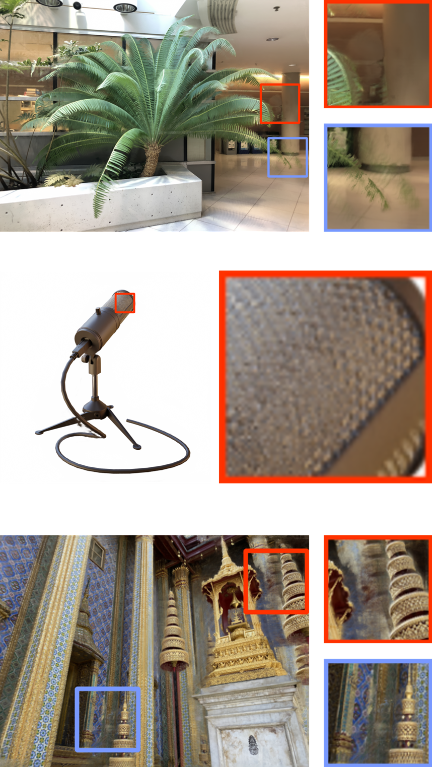
(a) IBRNet

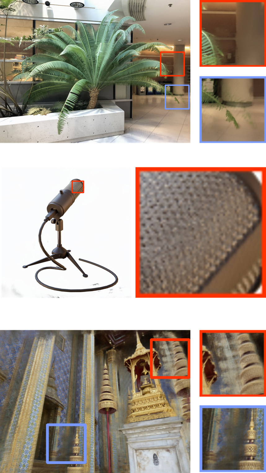
(b) GNT

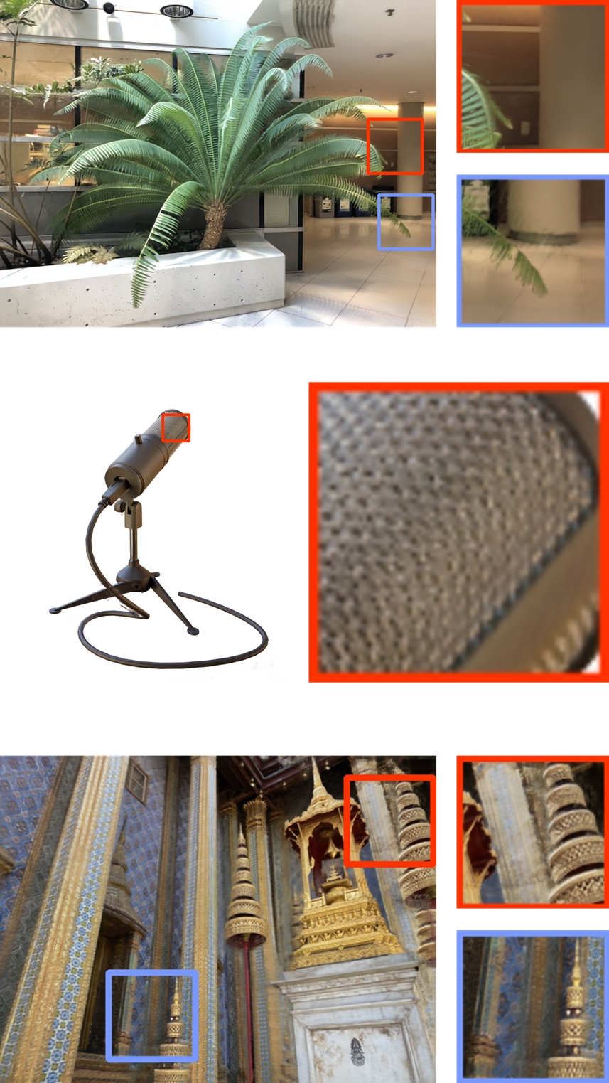
(c) EVE-NeRF

Figure 4: Qualitative comparison of EVE-NeRF with IBRNet[41] and GNT[38] in setting 1. The first, second, and third rows correspond to the Fern scene from LLFF, the Mic scene from Blender, and the Crest scene from Shiny, respectively. Our method, EVE-NeRF, demonstrates superior capability compared to the baselines in accurately reconstructing the geometry, appearance, and complex texture regions. In particular, our method successfully reconstructs the leaves and the surrounding area in the Fern scene.

Method		LLFF			Blender			Shiny
	PSNR$\uparrow$	SSIM$\uparrow$	LPIPS$\downarrow$	PSNR$\uparrow$	SSIM$\uparrow$	LPIPS$\downarrow$	PSNR$\uparrow$	SSIM$\uparrow$	LPIPS$\downarrow$
PixelNeRF [48]	18.66	0.588	0.463	22.65	0.808	0.202	-	-	-
IBRNet [41]	25.17	0.813	0.200	26.73	0.908	0.101	23.60	0.785	0.180
GPNR [32]	25.35	0.818	0.198	28.29	0.927	0.080	25.72	0.880	0.175
NeuRay [23]	25.72	0.880	0.175	26.48	0.944	0.091	24.12	0.860	0.170
GNT [38]	25.53	0.836	0.178	26.01	0.925	0.088	27.19	0.912	0.083
EVE-NeRF	27.16	0.912	0.134	27.03	0.952	0.072	28.01	0.935	0.083

Table 1: Results for setting 1. Our proposed method, EVE-NeRF, outperforms most of the baselines on the majority of the metrics. With the exception of PixelNeRF [48], all baseline methods [41, 32, 23] employ sequential or independent transformer-based single-dimensional ray aggregation. In contrast, our approach is based on a dual-branch structure, enabling multi-dimensional interactions for both view and epipolar information. The results confirm that our method’s multi-dimensional ray feature aggregation is superior to the single-dimensional aggregation used in the baselines.

Setting 1: Generalizable NVS.  Following IBRnet [41], we set up the reference view pool comprising $k\times M$ proximate views. $M$ views are chosen at random from this pool to serve as source views. Throughout the training process, the parameters $k$ and $M$ are subject to uniform random sampling, with $k$ drawn from $(1,3)$ and $M$ from $(8,12)$. During evaluation, we fix the number of source views $M=10$.

For the training dataset, we adopt object renderings of $1,030$ models from Google Scanned Object [12], RealEstate10K [51], $100$ scenes from the Spaces dataset [13] and $95$ real scenes from handheld cellphone captures [24, 41]. For the evaluation dataset, we use Real Forward-Facing [24], Blender [25] and Shiny [43].

Table 1 presents the quantitative results, while Figure 4 showcases the qualitative results. As shown in Table 1, comparison to methods [41, 32, 23] using transformer networks for feature aggregation, our approach outperforms them under most metrics. Our method outperforms SOTA method GNT [38] by $4.43\%$$\uparrow$ PSNR, $4.83\%$$\uparrow$ SSIM, $14.3\%$$\downarrow$ LPIPS in 3 evaluating dataset evenly. Such results verify the effectiveness of introducing the complementary appearance continuity and geometry consistency priors to the feature aggregation. Additionally, as shown in the second row of Figure 4, our method successfully reconstructs intricate textural details.

Setting 2: Few-Shot NVS.  To compare with few-shot generalizable neural rendering methods [4, 7], we conducted novel view synthesis experiments with $M=3$ input views in both training and evaluating, following the MVSNeRF [4] setting. We split the DTU [18] dataset into 88 scenes for training and 16 scenes for testing, following the methodology of prior works. Additionally, we also conducted training on the Google Scanned Object dataset. As shown in Table 6.2, we performed a quantitative comparison with 4 few-shot generalizable neural rendering methods [48, 41, 4, 7] on the DTU testing dataset and Blender. With only 3 source views input for setting, our model still achieves good performance. Our method outperforms SOTA methods MatchNeRF [7] by $2.19\%$$\uparrow$ PSNR, $13.0\%$$\downarrow$ LPIPS in 2 evaluating dataset evenly. Please refer to Appendix D.1 for the qualitative comparison for setting 2.

Efficiency Comparison.  As shown in the Figure 6.2, our method is compared with GNT [38] and GPNR [32] in terms of efficiency. We perform the testing of setting 1 in LLFF dataset. The result illustrates that our method not only requires less memory and faster rendering time per-image, but also has a higher PSNR for novel view synthesis.

Method		DTU			Blender
	PSNR$\uparrow$	SSIM$\uparrow$	LPIPS$\downarrow$	PSNR$\uparrow$	SSIM$\uparrow$	LPIPS$\downarrow$
PixelNeRF [48]	19.31	0.789	0.671	7.39	0.658	0.411
IBRNet [41]	26.04	0.917	0.190	22.44	0.874	0.195
MVSNeRF [4]	26.63	0.931	0.168	23.62	0.897	0.176
MatchNeRF [7]	26.91	0.934	0.159	23.20	0.897	0.164
EVE-NeRF	27.80	0.937	0.149	23.45	0.903	0.132

Table 2: Results for setting 2. Our method (EVE-NeRF) is trained on DTU and the Google Scanned Object dataset with 3 reference views. Our method outperforms on multiple metrics with other few-shot generalizable neural rendering methods.

Model	Storage$\downarrow$	Time$\downarrow$	PSNR$\uparrow$
GNT [38]	112MB	208s	25.35
GPNR [32]	110MB	12min	25.53
EVE-NeRF	53.8MB	194s	27.16

Table 3: Efficiency comparison results in LLFF dataset on the same RTX4090. Our method requires less storage, shorter rendering time per new view synthesis, and higher quality reconstruction compared to GNT [38] and GPNR [32].

6.3 Ablation Studies

To evaluate the significance of our contributions, we conducted extensive ablation experiments. We trained on setting 1 and tested on the Real Forward-Facing dataset. For efficiency, in both the training and testing datasets we set the resolutions of images reduced by half in both the training and testing datasets, resulting in the resolution of $504\times 378$ for the Real Forward-Facing dataset.

Only view/epipolar transformer.  In this ablation, we maintain only the view/epipolar transformers and NeRF decoder. As can be observed in the first row of Table 4, using only view/epipolar transformer reduces PSNR by $6.21\%$ compared to EVE-NeRF due to the limitations of view/epipolar aggregation in only one dimension.

Along-epipolar perception.  Compared with only view transformer, we retained view transformer with along-epipolar perception in this ablation. As shown in Table 4 and Figure 3, using along-epipolar perception would increase PSNR by $1.80\%$. The appearance continuity prior provided by along-epipolar perception compensates for the missing epipolar information in the pure view aggregation model.

Multi-view calibration.  Similarly, against to only epipolar transformer, we kept the epipolar transformer with multi-view calibration. As can be observed in Table 4 and Figure 3, adopting multi-view calibration would improve the performance of generalizable rendering. It verifies that the multi-view calibration can enhance epipolar aggregating ability via geometry prior.

Naïve dual network architecture.  To validate the effectiveness of our proposed entangled aggregation, we compared our EVE-NeRF with two other architectures: the Naïve Dual Transformer and the Dual Transformer with Cross-Attention Interaction (see Appendix A.4). Our method outperforms both naïve dual transformer by $3.85\%$ and $3.14\%$ PSNR. Visualization results are provided in Appendix D.4. It is demonstrated that our proposed EVE-NeRF has a robust ability to fusing view and epipolar pattern.

Model	PSNR$\uparrow$	SSIM$\uparrow$	LPIPS$\downarrow$
only view transformer	25.03	0.886	0.132
+ along-epipolar perception	25.48	0.892	0.128
only epipolar transformer	25.02	0.879	0.147
+ multi-view calibration	25.17	0.883	0.141
naïve dual transformer	25.66	0.890	0.128
+ cross-attention interaction	25.85	0.896	0.120
EVE-NeRF	26.69	0.913	0.102

Table 4: Ablations. The ablation study was conducted by training in a low-resolution setting 1 and testing on LLFF dataset with the resolution of $504\times 378$.

6.4 Visualization on Entangled Information Interaction

To further validate the entangled information interaction module’s ability of providing the de facto appearance continuity prior and geometry consistency prior, we visualize and analyze the the importance weights predicted by the along-epipolar perception and multi-view calibration.

The along-epipolar perception provides appearance continuity prior and regresses the importance weights for the target ray’s sampled depths. Specifically, we obtain a depth map by multiplying the depth weights with the marching distance along the ray. As shown in Figure 5, the adjacent-depth attention map demonstrates a more coherent character, indicating that the along-epipolar perception provides beneficial appearance consistency prior.

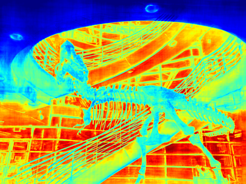
(a) Adjacent-depth attention map

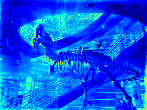
(b) Rendered depth map

Figure 5: Visualizations of adjacent-depth attention map and rendered depth map. By capitalizing on the appearance continuity prior, adjacent-depth attention boosts the coherence in depth map.

The multi-view calibration provides geometry consistency prior and predicts the importance weights for the source views. We use particular color to represent the source view with the highest relevance to the target pixel, which corresponds to the index with the largest output value from the multi-view calibration. As shown in Figure 6, the view transformer and the multi-view calibration correctly predict the correspondence between the target pixel and the source views, such as the back of the chair. Furthermore, both methods predict that the pixels in the upper right part of the chair correspond to source view 3, where the upper right part of the chair is occluded. We believe that EVE-NeRF learns about the awareness of visibility, even when the target pixel is occluded.

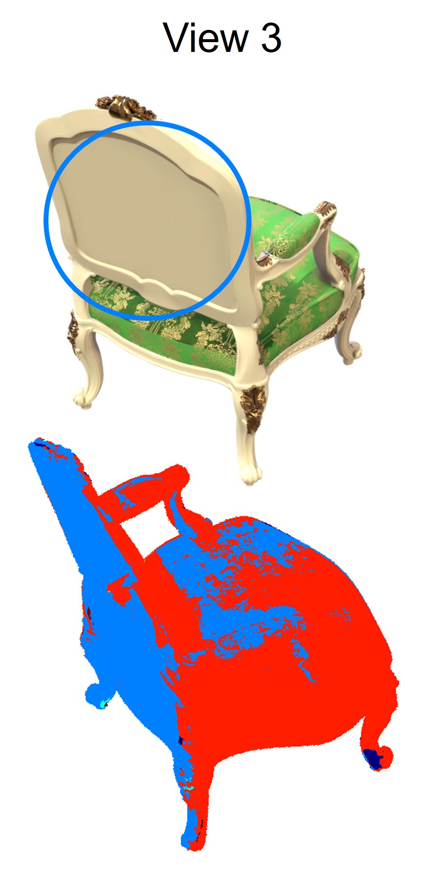
(a) View Transformer

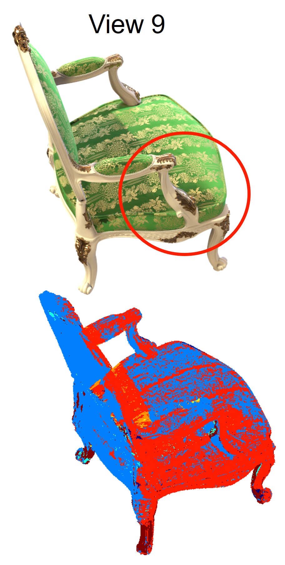
(b) Multi-View Calibration

(c)

Figure 6: Each color represents the source view ID corresponding to the maximum weight for the target pixel. Both the view transformer and the multi-view calibration have successfully learned the cross-view information from the source views.

7 Conclusion

We propose a new Generalizable NeRF named EVE-NeRF that aggregates cross-view and along-epipolar information in an entangled manner. The core of EVE-NeRF consists of our new proposed View Epipolar Interaction Module (VEI) and Epipolar View Interaction Module (EVI) that are organized alternately. VEI and EVI can project the scene-invariant appearance continuity and geometry consistency priors, which serve to offset information losses that typically arises from single-dimensional aggregation operations. We demonstrate the superiority of our method in both generalizable and few-shot NVS settings compared with the state-of-the-art methods. Additionally, extensive ablation studies confirm that VEI and EVI can enhance information interaction across view and epipolar dimension to yield better generalizable 3D representation.

Appendix A Implementation Details

A.1 Generalizable 3D Representation $\boldsymbol{z}$

EVE-NeRF alternates the aggregation of epipolar and view dimensions’ features through the VEI and EVI modules, resulting in the generation of generalizable 3D representation $\boldsymbol{z}$ that aligns with NeRF’s coordinates. The pseudocode for the computation of $\boldsymbol{z}$ is as follows:

Input: viewpoints difference $\Delta\boldsymbol{d}^{s}$, extracted convolution features $\boldsymbol{f}^{c}\in\mathbb{R}^{N\times M\times C}$, numbers of aggregation module $N_{layer}$

Output: generalizable 3D representation $\boldsymbol{z}$

1

2$\boldsymbol{X}=\boldsymbol{f}^{c}$;

3 $i=1$;

4 while $i\leq N_{layer}$ do

5       $\boldsymbol{h}=\boldsymbol{X}$;

6       $\boldsymbol{Q}=\boldsymbol{X}\boldsymbol{W_{Q}},\boldsymbol{K}=\boldsymbol{X}\boldsymbol{W_{K}},\boldsymbol{V}=\boldsymbol{X}\boldsymbol{W_{V}}$;

7       $\boldsymbol{X}=\text{VEI}\left(\boldsymbol{Q},\boldsymbol{K},\boldsymbol{V},\Delta\boldsymbol{d}^{s}\right)$;

8       $\boldsymbol{Mean},\boldsymbol{Var}=\text{mean\&var}\left(\boldsymbol{V},\text{dim}=1\right)$;

9       $\boldsymbol{w}^{v}=\text{sigmoid}\left(\text{AE}\left(\boldsymbol{Mean},\boldsymbol{Var}\right)\right)$;

10       $\boldsymbol{X}=\boldsymbol{X}\cdot\boldsymbol{w}^{v}$;

11       $\boldsymbol{X}^{\prime}=\boldsymbol{X.}\text{permute}\left(1,0,2\right)$;

12       $\boldsymbol{Q}^{\prime}=\boldsymbol{X}^{\prime}\boldsymbol{W^{\prime}_{Q}},\boldsymbol{K}^{\prime}=\boldsymbol{X}^{\prime}\boldsymbol{W^{\prime}_{K}},\boldsymbol{V}^{\prime}=\boldsymbol{X}^{\prime}\boldsymbol{W^{\prime}_{V}}$;

13       $\boldsymbol{X}^{\prime}=\text{EVI}\left(\boldsymbol{Q}^{\prime},\boldsymbol{K}^{\prime},\boldsymbol{V}^{\prime},\Delta\boldsymbol{d}^{s}\right)$;

14       $\boldsymbol{Max}=\text{max}\left(\boldsymbol{V}^{\prime},\text{dim}=1\right)$;

15       $\boldsymbol{w}^{e}=\text{sigmoid}\left(\text{self-attn}\left(\boldsymbol{Max}\right)\right)$;

16       $\boldsymbol{X}^{\prime}=\boldsymbol{X}^{\prime}\cdot\boldsymbol{w}^{e}$;

17       $\boldsymbol{X}=\boldsymbol{X}^{\prime}.\text{permute}\left(1,0,2\right)+\boldsymbol{h}$;

18       $i=i+1$;

19      

20 end while

21$\boldsymbol{z}=\text{mean}(\boldsymbol{X},\text{dim}=1)\in\mathbb{R}^{N\times C}$;

22

Algorithm 1 EVE-NeRF:PyTorch-like Pseudocode

A.2 Difference of Views $\Delta\boldsymbol{d}^{s}$

$\Delta\boldsymbol{d}^{s}$ serves as an additional input to attention computation in the view transformer and the epipolar transformer, allowing the model to learn more information about the differences in views. The pseudo-code for computing $\Delta\boldsymbol{d}^{s}$ is shown in Algorithm 2.

Input: the target ray direction $\boldsymbol{d}_{t}\in\mathbb{R}^{3}$, the source ray direction $\boldsymbol{d}_{s}\in\mathbb{R}^{M\times 3}$ , the number of sampling points along the target ray $N$

Output: $\Delta\boldsymbol{d}^{s}$

1

2$\boldsymbol{d}_{t}=\boldsymbol{d}_{t}.\text{unsqueeze}(0).\text{repeat}(M,1)$;

3 $\boldsymbol{d}_{diff}=\boldsymbol{d}_{t}-\boldsymbol{d}_{s}$;

4 $\boldsymbol{d}_{diff}=\boldsymbol{d}_{diff}/\text{torch.norm}(\boldsymbol{d}_{diff},\text{dim}=-1,\text{keepdim=True})$;

5 $\boldsymbol{d}_{dot}=\text{torch.sum}(\boldsymbol{d}_{t}*\boldsymbol{d}_{s}$;

6 $\boldsymbol{\Delta\boldsymbol{d}^{s}}=\text{torch.cat}([\boldsymbol{d}_{diff},\boldsymbol{d}_{dot}],\text{dim}=-1)$;

7 $\boldsymbol{\Delta\boldsymbol{d}^{s}}=\boldsymbol{\Delta\boldsymbol{d}^{s}}.\text{unsqueeze}(0).\text{repeat}(N,1,1)\in\mathbb{R}^{N\times M\times 4}$;

8

Algorithm 2 $\Delta\boldsymbol{d}^{s}$:PyTorch-like Pseudocode

A.3 Difference of Camera Poses $\Delta\boldsymbol{pose}$

$\Delta\boldsymbol{pose}$ provides camera disparity information for multi-view calibration, which is merged with epipolar aggregation features to obtain geometry consistency prior. The pseudo-code to compute $\Delta\boldsymbol{pose}$ is shown in Algorithm 3.

Input: the target pose matrix $\boldsymbol{P}_{t}\in\mathbb{R}^{3\times 4}$, the source pose matrix $\boldsymbol{P}_{s}\in\mathbb{R}^{M\times 3\times 4}$

Output: $\Delta\boldsymbol{pose}$

1

2$M=\boldsymbol{P}_{s}.shape[0]$;

3 $\boldsymbol{P}_{t}=\boldsymbol{P}_{t}$.unsqueeze(dim=0).repeat($M,1,1$);

4 $\boldsymbol{R}_{t}=\boldsymbol{P}_{t}[:,:3,:3]$;

5 $\boldsymbol{R}_{s}=\boldsymbol{P}_{s}[:,:3,:3]$;

6 $\boldsymbol{T}_{t}=\boldsymbol{P}_{t}[:,:3,-1]$;

7 $\boldsymbol{T}_{s}=\boldsymbol{P}_{s}[:,:3,-1]$;

8 $\Delta\boldsymbol{R}=\boldsymbol{R}_{t}\text{@}\boldsymbol{R}_{s}^{T}.\text{view}(M,9)$;

9 $\Delta\boldsymbol{T}=\boldsymbol{T}_{t}-\boldsymbol{T}_{s}^{T}$;

10 $\Delta\boldsymbol{pose}=\text{torch.cat}([\Delta\boldsymbol{R},\Delta\boldsymbol{T}],\text{dim=-1})\in\mathbb{R}^{M\times 12}$;

11

Algorithm 3 $\Delta\boldsymbol{pose}$:PyTorch-like Pseudocode

A.4 Additional Technical Details

EVE-NeRF network details.  Our lightweight CNN consists of 4 convolutional layers with a kernel size of $3\times 3$ and a stride of 1. BatchNorm layers and ReLU activation functions are applied between layers. The final output feature map has a dimension of 32. The VEI and EVI modules have 4 layers, which are connected alternately. Both the View Transformer and Epipolar Transformer have the same network structure, in which the dimension of hidden features is 64 and we use 4 heads for the self-attention module in transformer layers. For the transformer in Multi-View Calibration, the features dimension is 64 and head is 4, consisting of 1 blocks. For the AE network in Along-Epipolar Perception and the conditioned NeRF decoder are set the same as the experimental setups of GeoNeRF [19] and IBRNet [41], respectively. The network architectures of the lightweight CNN, the AE network, and the conditioned NeRF decoder are provided in Table 5, 6, and 7 respectively.

Input	Layer	Output
Input	Conv2d(3, 32, 3, 1)+BN+ReLU	conv0
conv0	Conv2d(32, 32, 3, 1)+BN+ReLU	conv1
conv1	Conv2d(32, 32, 3, 1)+BN	conv$2\_0$
(conv0, conv$2\_0$)	Add(conv0, conv$2\_0$) + ReLU	conv$2\_1$
conv$2\_1$	Conv2d(32, 32, 3, 1)+BN+ReLU	conv3

Table 5: Network architecture of the lightweight CNN, where conv3 is the output features. Conv2d($c_{in}$, $c_{out}$, $k$, $s$) stands for a 2D convolution with input channels $c_{in}$, output channels $c_{out}$, kernel size of $k$, and stride of $s$. BN stands for Batch Normalization Layer. ReLU stands for ReLU nonlinearity activation function. Add(x, y) means add x and y.

Input	Layer	Output
Input	Conv1d(128, 64, 3, 1)+LN+ELU	conv$1\_0$
conv$1\_0$	MaxPool1d	conv1
conv1	Conv1d(64, 128, 3, 1)+LN+ELU	conv$2\_0$
conv$2\_0$	MaxPool1d	conv2
conv2	Conv1d(128, 128, 3, 1)+LN+ELU	conv$3\_0$
conv$3\_0$	MaxPool1d	conv3
conv3	TrpsConv1d(128, 128, 4, 2)+LN+ELU	x$\_$0
$[$conv2;x$\_$0$]$	TrpsConv1d(256, 64, 4, 2)+LN+ELU	x$\_$1
$[$conv1;x$\_$1$]$	TrpsConv1d(128, 32, 4, 2)+LN+ELU	x$\_$2
$[$Input;x$\_$2$]$	Conv1d(64, 64, 3, 1)+Sigmoid	output

Table 6: Network architecture of the 1D convolution AE. Conv2d($c_{in}$, $c_{out}$, $k$, $s$) stands for a 1D convolution with input channels $c_{in}$, output channels $c_{out}$, kernel size of $k$, and stride of $s$. LN stands for Layer Normalization Layer. ELU and Sigmoid stand for ELU and Sigmoid nonlinearity activation function separately. MaxPool1d is a 1D max pooling layer with a stride of 2. TrpsConv1d stands for transposed 1D convolution. $\left[\cdot;\cdot\right]$ means concatenation.

Input	Layer	Output
$\boldsymbol{z}$	Linear(64, 128)	bias
$\gamma(\boldsymbol{p})$	Linear(63, 128)	x0$\_$0
x0$\_$0,bias	Mul(x0$\_$0,bias)+ReLU	x0
x0	Linear(128, 128)	x1$\_$0
x1$\_$0,bias	Mul(x1$\_$0,bias)+ReLU	x1
x1	Linear(128, 128)	x2$\_$0
x2$\_$0,bias	Mul(x2$\_$0,bias)+ReLU	x2
x2	Linear(128, 128)	x3$\_$0
x3$\_$0,bias	Mul(x3$\_$0,bias)+ReLU	x3
x3	Linear(128, 128)	x4$\_$0
x4$\_$0,bias	Mul(x4$\_$0,bias)+ReLU	x4
$[$x4;$\gamma(\boldsymbol{p})]$	Linear(191, 128)	x5$\_$0
x5$\_$0,bias	Mul(x5$\_$0,bias)+ReLU	x5
x5	Linear(128, 16)+ReLU	alpha$\_$raw
alpha$\_$raw	Mul(4, 16)	alpha0
alpha0	Linear(16,16)+ReLU	alpha1
alpha1	Linear(16,1)+ReLU	alpha
$[$x5;$\gamma(\boldsymbol{d})]$	Linear(191,64)+ReLU	x6
x6	Linear(64, 3)+Sigmoid	rgb

Table 7: Network architecture of the conditioned NeRF decoder. $\boldsymbol{z}$, $\boldsymbol{p}$, and $\boldsymbol{d}$ stand for the generalizable features, the coordinates of 3D sampling points, and the directions of rays, individually. $\gamma$ stands for positional encoding in NeRF. Linear($c_{in},c_{out}$) stands for a linear layer with input channels $c_{in}$ and output channels $c_{out}$. Mul stands for element-wise multiplication. MHA($head,dim$) stands for a multi-head-attention layer with the number of head $head$ and attention dimension $dim$. $\left[\cdot;\cdot\right]$ means concatenation.

Naïve dual network details.  To further validate the rationality of EVE-NeRF’s dual-branch structure, in Sec 6.3, we compared our method with two naïve dual network architectures: the Naïve Dual Transformer and the Dual Transformer with Cross-Attention Interaction. The Naïve Dual Transformer’s first branch is GNT [38], and the second branch is GNT with epipolar aggregation followed by view aggregation. The outputs of both branches make color predictions via a tiny MLP network directly. Experiments with GNT demonstrated that using volume rendering to calculate color values does not enhance GNT’s performance. Hence, we consider it fair to compare EVE-NeRF with these two dual-branch networks. The Dual Transformer with Cross-Attention Interaction builds upon the Naïve Dual Transformer by adding a cross-attention layer for inter-branch interaction. These dual network architectures are illustrated in Figure 7.

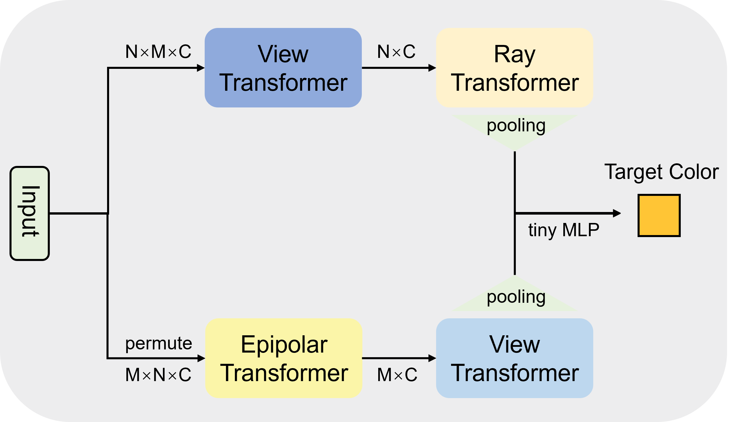
(a) Naïve Dual Transformer

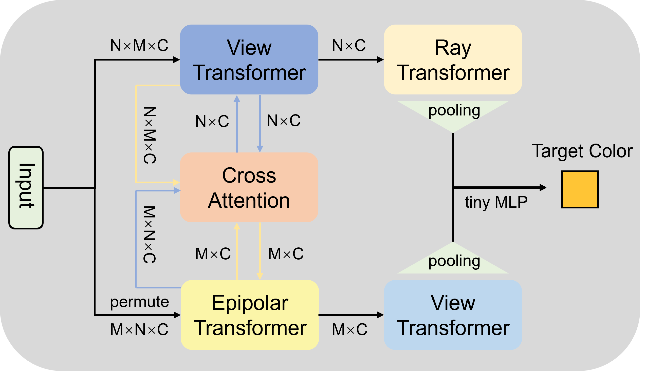
(b) w/ Cross-Attention Interaction

Figure 7: Naïve dual network architecture. We design 2 baselines of dual networks for comparison: a) the Naïve Dual Transformer and b) the Dual Transformer with Cross-Attention Interaction. Table 4 demonstrates that our proposed method, EVE-NeRF, exhibits superior generalization capabilities for novel view synthesis.

Appendix B Multi-View Epipolar-Aligned Feature Extraction

Let $\boldsymbol{K}_{t}$ and $\boldsymbol{P}_{t}=[\boldsymbol{R}_{t},\boldsymbol{t}_{t}]$ represent the camera intrinsic and extrinsic parameters for the target view, and let $\boldsymbol{u}_{t}$ be the pixel coordinates corresponding to the target ray $\mathcal{R}$. In this case, $\mathcal{R}$ can be parameterized in the world coordinate system based on the delta parameter as follows:

$$\mathcal{R}(\delta)=\boldsymbol{t}_{t}+\delta\boldsymbol{R}_{t}\boldsymbol{K}_{t}^{-1}[\boldsymbol{u}_{t}^{\top},1]^{\top}.$$ (12)

Next, we sample $N$ points$\{\boldsymbol{p}_{i}\}_{i=1}^{N}=\{\mathcal{R}(\delta_{i})\}_{i=1}^{N}$ along $\mathcal{R}$ and project them onto the $j$-th source view:

$$d_{j}^{i}[{u_{j}^{i}}^{\top},1]^{\top}=\boldsymbol{K}_{j}\boldsymbol{R}_{j}^{-1}(\boldsymbol{p}_{i}-\boldsymbol{t}_{j}),$$ (13)

where $u_{j}^{i}$ is the 2D coordinates of the $i$-th sampled point’s projection onto the $j$-th source view, and $d_{j}^{i}$ is the corresponding depth. Clearly, the projection points of these sampled points lie on the corresponding epipolar line in that view. Next, we obtain the convolution features $\boldsymbol{f}^{c}=\{\boldsymbol{f}^{c}_{i,j}\}_{i=1,j=1}^{N,M}$ in $\{\boldsymbol{F}_{i}^{c}\}_{i=1}^{M}$ for these projection points via bilinear interpolation. Therefore, for the target ray $\mathcal{R}$, we now have the multi-view convolution features $\boldsymbol{f}^{c}\in\mathbb{R}^{N\times M\times C}$ for $\mathcal{R}$, where $C$ is the number of channels in the convolution features.

(a) Ground Truth

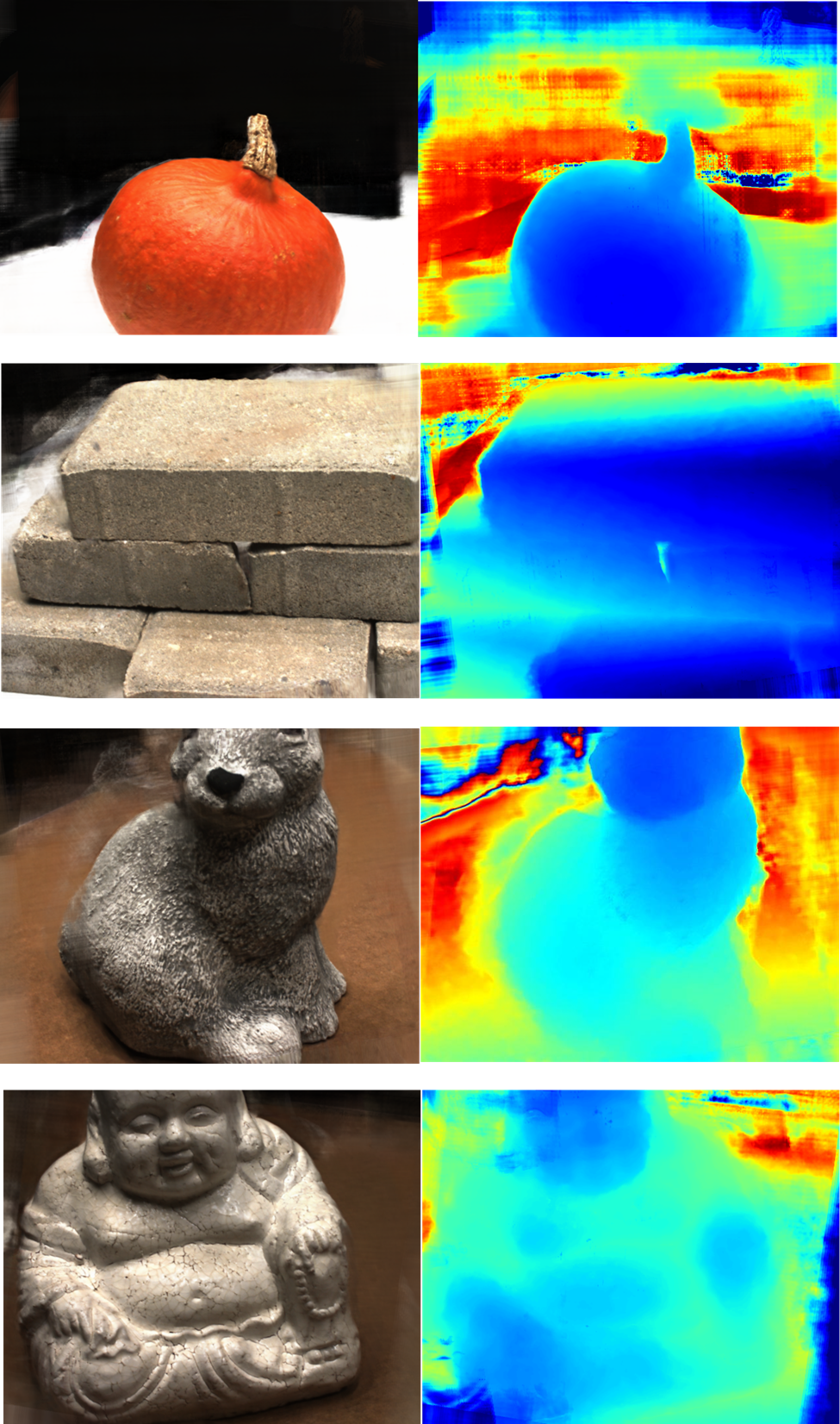
(b) MVSNeRF

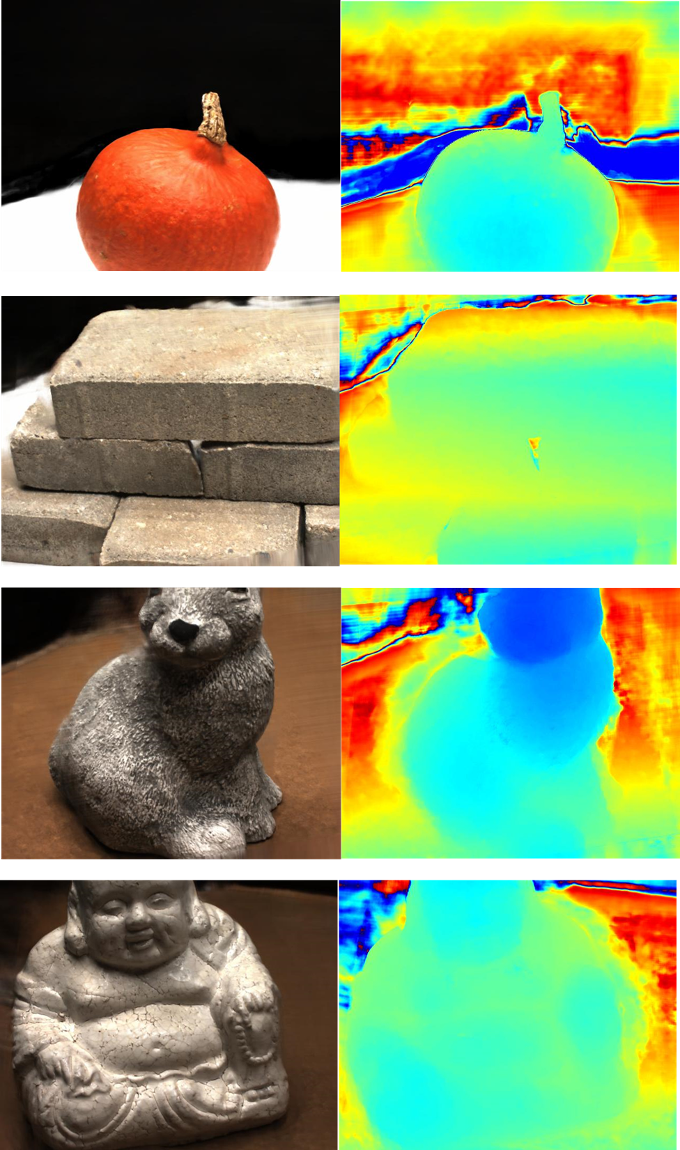
(c) MatchNeRF

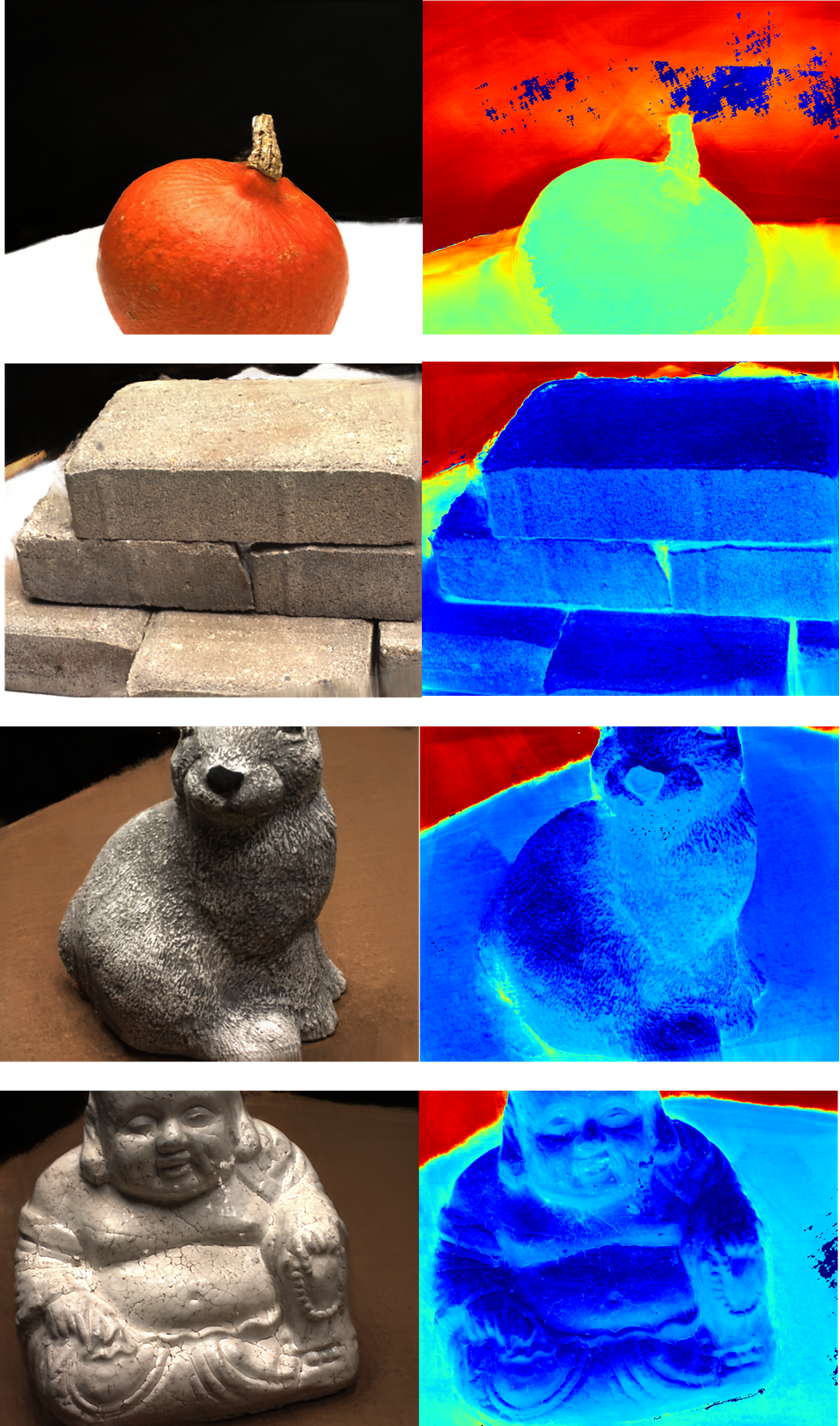
(d) EVE-NeRF

Figure 8: Qualitative comparison of our generalizable GeoNeRF model with MVSNeRF [4] and MatchNeRF [7] in the few-shot setting. Our proposed method, EVE-NeRF, not only has higher rendering of new view pictures but also provides more accurate and detailed depth maps (without ground-truth depth supervision).This is due to the fact that EVE-NeRF provides accurate geometric and appearance a prior of multiple views for the model through the complementary structure of epipolar aggregation and view aggregation.

(a) Branch1 Rendering Results

(b) Branch2 Rendering Results

Figure 9: Qualitative comparison with dual branches within the Naïve Dual Transformer

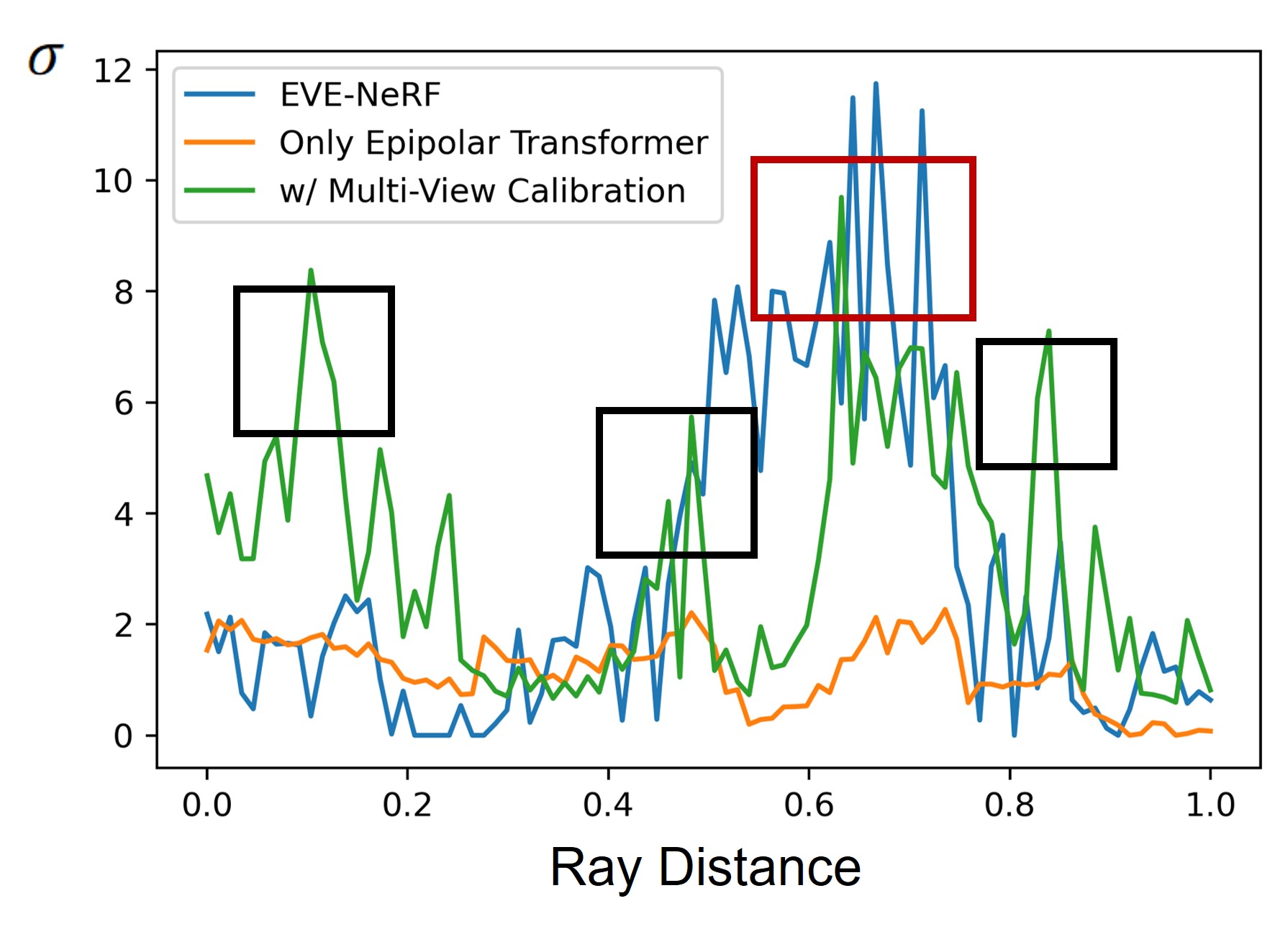
(a) Volume density of ray 1

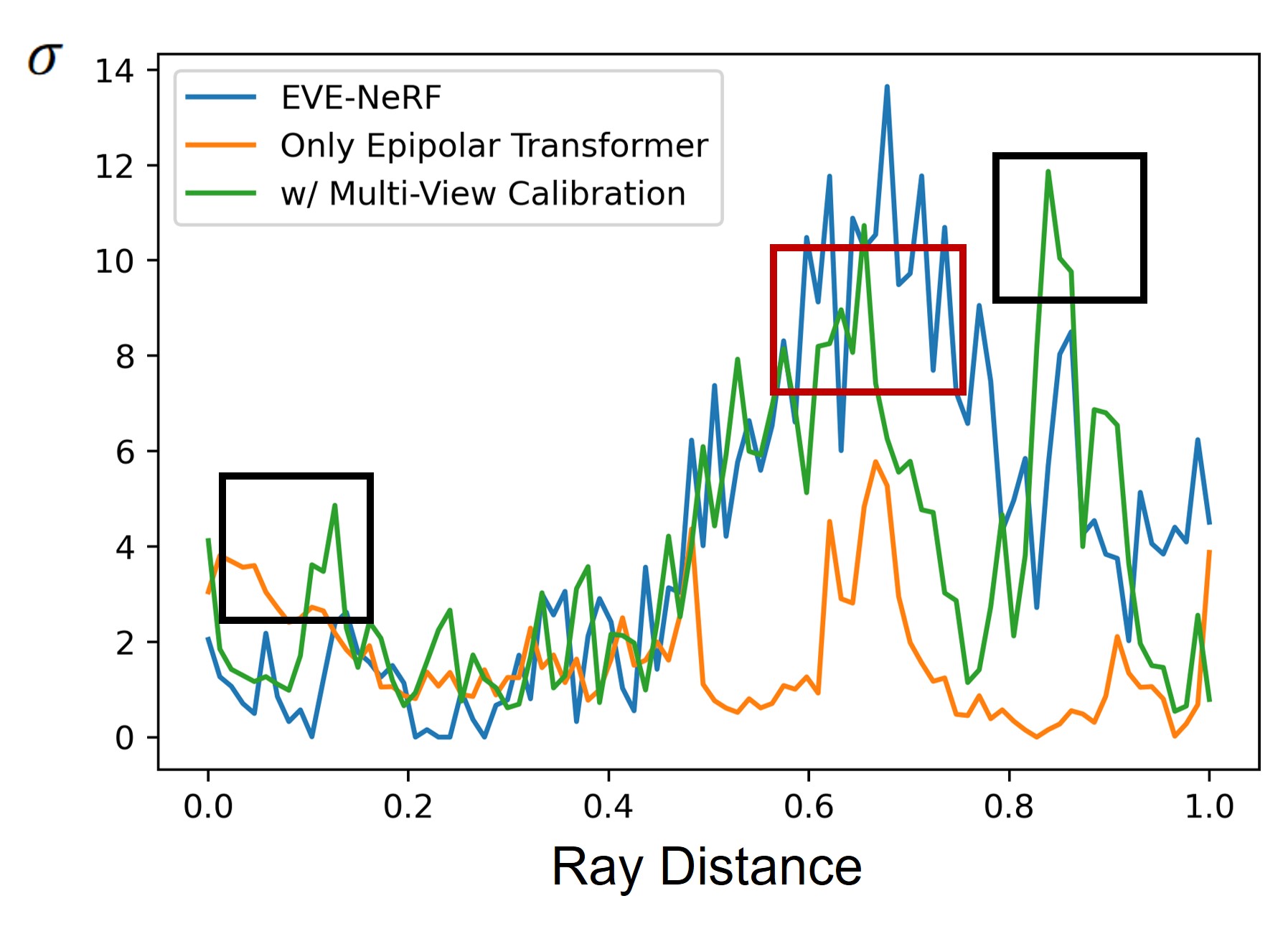
(b) Volume density of ray 2

Figure 10: Line charts of the volume density from a novel view of the Chair scene in Blender [25]. Red boxes represent correct peaks and black boxes represent abnormal peaks. Multi-View Calibration learns more complex signals but with more noise. Volume densities predicted by EVE-NeRF are more likely to have a single-peak distribution.

Appendix C Feature Aggregation Network Proposed in Other Domains

Dual-branch network structures are commonly used in computer vision tasks [31, 42, 6, 9]. For instance, Simonyan [31] introduced a dual-stream network for action recognition in videos, consisting of a temporal stream for optical flow data and a spatial stream for RGB images, with the outputs from both branches being fused in the end. CrossVIT [6] is a visual Transformer model based on dual branches, designed to enable the model to learn multi-scale feature information by processing different-sized image patches through the dual-branch network. DAT [9], on the other hand, is a transformer-based image super-resolution network that aggregates spatial and channel features through alternating spatial window self-attention and channel self-attention, enhancing representation capacity. Our approach does not follow the naive dual-branch structure. Instead, we introduce the along-epipolar perception and the multi-view calibration to compensate for the shortcomings in information interaction of the other branch. Besides, our dual-branch network demonstrates the efficient interplay between branches.

Appendix D Additional Results

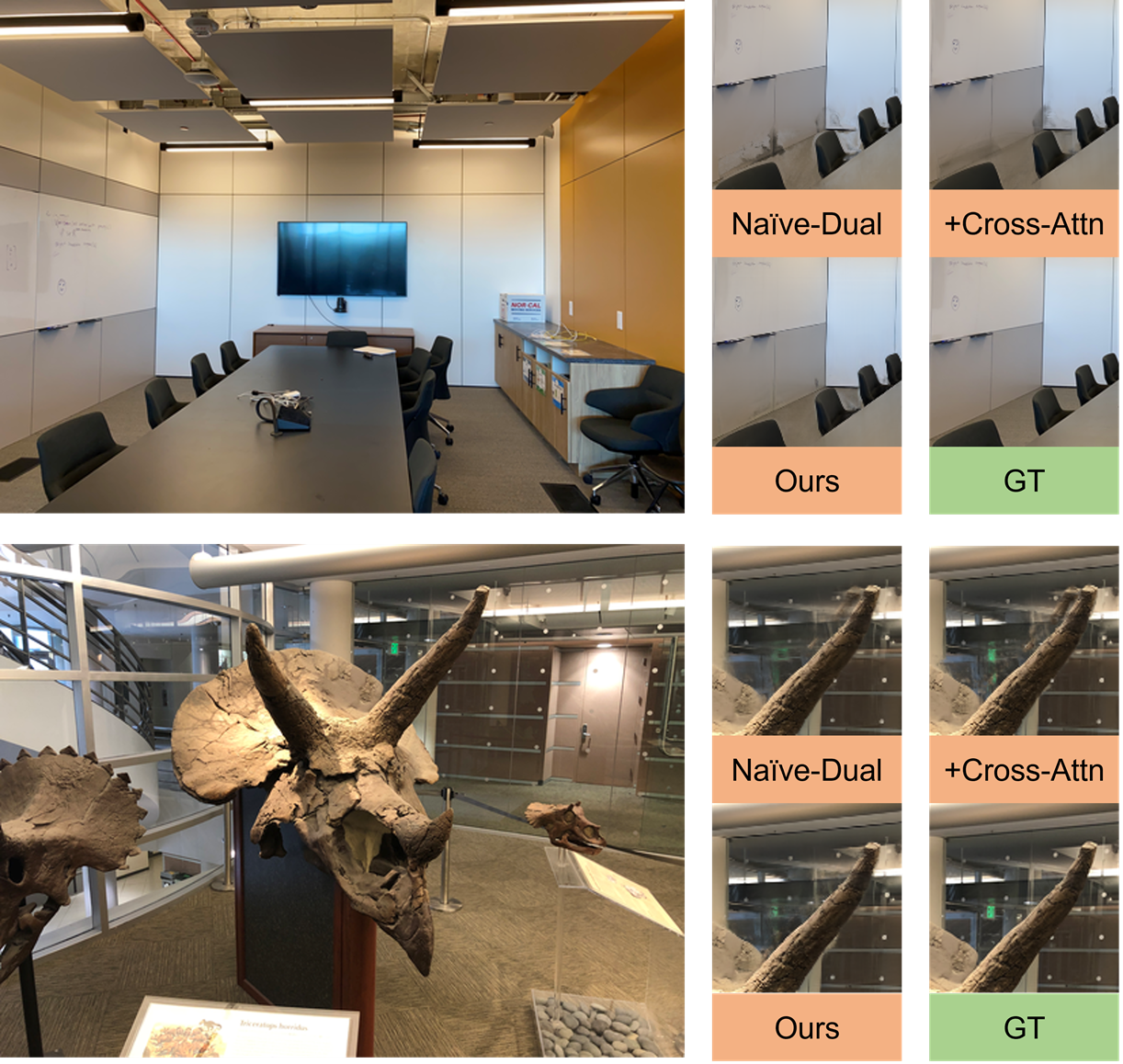
(a) LLFF datasets

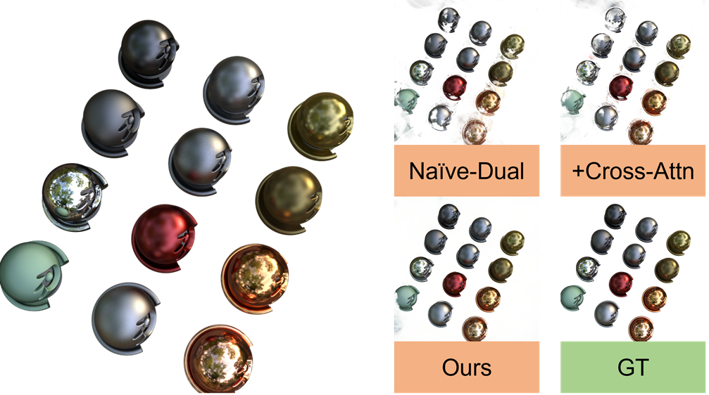
(b) Blender datasets

Figure 11: Qualitative comparison with naïve dual network architectures.

D.1 Qualitative Comparison for Setting 2

A qualitative comparison of our method with the few-shot generalizable neural rendering methods [4, 7] is shown in Figure 8. The novel view images rendered by our method produce minimal artifacts and can render the edge portion of the image and weakly textured regions. In addition, we generate a novel view depth map with 3 source views input through the volume rendering [25]. From Figure 8 we can observe that our generated depth map is more accurate and precise in terms of scene geometry prediction. This indicates that our proposed EVE-NeRF can extract high-quality aggregated features that imply the geometry and appearance of the scene, even in a few-shot setting.

D.2 Volume Density based on Geometry Consistency Prior

As shown in Figure 10, we visualize two line charts of the point density. Multi-view calibration learns more complex light signals, but with a multi-peaked distribution. EVE-NeRF predicts point density distributions with distinct peaks and reduced noise in the light signals.

D.3 Per-Scene Fine-Tuning Results

Models	Room	Fern	Leaves	Fortress	Orchids	Flower	T-Rex	Horns	Avg
NeRF [25]	32.70	25.17	20.92	31.16	20.36	27.40	26.80	27.45	26.50
NeX [43]	32.32	25.63	21.96	31.67	20.42	28.90	28.73	28.46	27.26
NLF [33]	34.54	24.86	22.47	33.22	21.05	29.82	30.34	29.78	28.26
EVE-NeRF	33.97	25.73	23.78	32.97	21.27	29.06	29.18	30.53	28.31

(a) PSNR$\uparrow$

Models	Room	Fern	Leaves	Fortress	Orchids	Flower	T-Rex	Horns	Avg
NeRF [25]	0.948	0.792	0.690	0.881	0.641	0.827	0.880	0.828	0.811
NeX [43]	0.975	0.887	0.832	0.952	0.765	0.933	0.953	0.934	0.904
NLF [33]	0.987	0.886	0.856	0.964	0.807	0.939	0.968	0.957	0.921
EVE-NeRF	0.983	0.894	0.891	0.961	0.797	0.935	0.960	0.961	0.923

(b) SSIM$\uparrow$

Models	Room	Fern	Leaves	Fortress	Orchids	Flower	T-Rex	Horns	Avg
NeRF [25]	0.178	0.280	0.316	0.171	0.321	0.219	0.249	0.268	0.250
NeX [43]	0.161	0.205	0.173	0.131	0.242	0.150	0.192	0.173	0.178
NLF [33]	0.104	0.135	0.110	0.119	0.173	0.107	0.143	0.121	0.127
EVE-NeRF	0.060	0.140	0.119	0.089	0.186	0.103	0.095	0.086	0.110

(c) LPIPS$\downarrow$

Table 8: Single-scene fine-tuned comparison results for the LLFF dataset

We fine-tune for $60,000$ iterations for each scene on the LLFF dataset. The quantitative comparison of our method with single-scene NeRF is demonstrated as shown in Table 8. We compare our method EVE-NeRF with NeRF [25], NeX [43], and NLF [33]. Our method outperforms baselines on the average metrics. The LPIPS of our method is lower than NLF by $13.4\%$, although NLF requires larger batchsize and longer iterations of training.

D.4 Qualitative Comparison With Naïve Dual Network Methods

As depicted in Figure 11(a), we showcase a qualitative comparison of our approach with two other dual-branch methods on the Room and Horns scenes from the LLFF dataset. Our approach exhibits fewer artifacts and a more accurate geometric appearance. Specifically, in the Room scene, our method avoids the black floating artifacts seen in the chair and wall in the other two methods. In the Horns scene, our approach accurately reconstructs the sharp corners without causing ghosting effects. Figure 11(b) illustrates the qualitative comparison results in the Materials scene from the Blender dataset. It is evident that our method outperforms other dual-branch methods in rendering quality.

While adding the cross-attention interaction mechanism can enhance the performance of generalizable new view synthesis, it is apparent from Figure 11 that the rendered novel view images still exhibit artifacts and unnatural geometry. In some cases, the reconstruction quality of certain objects may even be inferior to the naïve dual transformer, as observed in the upper-left part of Figure 11(b). This could be attributed to the limitation of the cross-attention interaction mechanism in aggregating features across both epipolar and view dimensions simultaneously.

Furthermore, we individually visualized the rendering results of each branch within the Naïve Dual Transformer, as depicted in Figure 9. It was observed that the second branch based on the epipolar transformer produced blurry rendering results. This is likely due to the absence of geometric priors, as interacting with epipolar information first can make it challenging for the model to acquire the geometry of objects. Therefore, aggregating view-epipolar feature naïvely may cause pattern conflict between view dimension and epipolar dimension. Our proposed EVE-NeRF differs from the naïve dual-branch structure in the sense that the second branch’s role is not to output generalizable aggregate features as the first branch does. Instead, it aims to compensate for the inadequacies in the first branch’s interaction with information in the epipolar or view dimensions, providing the appearance continuity prior and the geometry consistency priors.

Appendix E Limitation

Although our approach achieves superior performance in cross-scene novel view synthesis, it takes about 3 minutes to render a new view image with a resolution of $1008\times 756$, which is much longer than the vanilla scene-specific NeRF approach [25, 15, 8]. Nevertheless, we must admit that the simultaneous achievement of high-quality, real-time, and generalizable rendering poses a considerable challenge. In light of this, we posit that a potential avenue for further exploration is optimizing the speed of generalizable NeRF.

References

- Barron et al. [2021] Jonathan T Barron, Ben Mildenhall, Matthew Tancik, Peter Hedman, Ricardo Martin-Brualla, and Pratul P Srinivasan. Mip-nerf: A multiscale representation for anti-aliasing neural radiance fields. In Proceedings of the IEEE/CVF International Conference on Computer Vision, pages 5855–5864, 2021.
- Barron et al. [2022] Jonathan T Barron, Ben Mildenhall, Dor Verbin, Pratul P Srinivasan, and Peter Hedman. Mip-nerf 360: Unbounded anti-aliased neural radiance fields. In Proceedings of the IEEE/CVF Conference on Computer Vision and Pattern Recognition, pages 5470–5479, 2022.
- Barron et al. [2023] Jonathan T Barron, Ben Mildenhall, Dor Verbin, Pratul P Srinivasan, and Peter Hedman. Zip-nerf: Anti-aliased grid-based neural radiance fields. arXiv preprint arXiv:2304.06706, 2023.
- Chen et al. [2021a] Anpei Chen, Zexiang Xu, Fuqiang Zhao, Xiaoshuai Zhang, Fanbo Xiang, Jingyi Yu, and Hao Su. Mvsnerf: Fast generalizable radiance field reconstruction from multi-view stereo. In Proceedings of the IEEE/CVF International Conference on Computer Vision, pages 14124–14133, 2021a.
- Chen et al. [2022] Anpei Chen, Zexiang Xu, Andreas Geiger, Jingyi Yu, and Hao Su. Tensorf: Tensorial radiance fields. In European Conference on Computer Vision, pages 333–350. Springer, 2022.
- Chen et al. [2021b] Chun-Fu Richard Chen, Quanfu Fan, and Rameswar Panda. Crossvit: Cross-attention multi-scale vision transformer for image classification. In Proceedings of the IEEE/CVF international conference on computer vision, pages 357–366, 2021b.
- Chen et al. [2023a] Yuedong Chen, Haofei Xu, Qianyi Wu, Chuanxia Zheng, Tat-Jen Cham, and Jianfei Cai. Explicit correspondence matching for generalizable neural radiance fields. arXiv preprint arXiv:2304.12294, 2023a.
- Chen et al. [2023b] Zhiqin Chen, Thomas Funkhouser, Peter Hedman, and Andrea Tagliasacchi. Mobilenerf: Exploiting the polygon rasterization pipeline for efficient neural field rendering on mobile architectures. In Proceedings of the IEEE/CVF Conference on Computer Vision and Pattern Recognition, pages 16569–16578, 2023b.
- Chen et al. [2023c] Zheng Chen, Yulun Zhang, Jinjin Gu, Linghe Kong, Xiaokang Yang, and Fisher Yu. Dual aggregation transformer for image super-resolution. In Proceedings of the IEEE/CVF International Conference on Computer Vision, pages 12312–12321, 2023c.
- Chibane et al. [2021] Julian Chibane, Aayush Bansal, Verica Lazova, and Gerard Pons-Moll. Stereo radiance fields (srf): Learning view synthesis for sparse views of novel scenes. In Proceedings of the IEEE/CVF Conference on Computer Vision and Pattern Recognition, pages 7911–7920, 2021.
- Cong et al. [2023] Wenyan Cong, Hanxue Liang, Peihao Wang, Zhiwen Fan, Tianlong Chen, Mukund Varma, Yi Wang, and Zhangyang Wang. Enhancing nerf akin to enhancing llms: Generalizable nerf transformer with mixture-of-view-experts. In Proceedings of the IEEE/CVF International Conference on Computer Vision, pages 3193–3204, 2023.
- Downs et al. [2022] Laura Downs, Anthony Francis, Nate Koenig, Brandon Kinman, Ryan Hickman, Krista Reymann, Thomas B McHugh, and Vincent Vanhoucke. Google scanned objects: A high-quality dataset of 3d scanned household items. In 2022 International Conference on Robotics and Automation (ICRA), pages 2553–2560. IEEE, 2022.
- Flynn et al. [2019] John Flynn, Michael Broxton, Paul Debevec, Matthew DuVall, Graham Fyffe, Ryan Overbeck, Noah Snavely, and Richard Tucker. Deepview: View synthesis with learned gradient descent. In Proceedings of the IEEE/CVF Conference on Computer Vision and Pattern Recognition, pages 2367–2376, 2019.
- Gao et al. [2021] Chen Gao, Ayush Saraf, Johannes Kopf, and Jia-Bin Huang. Dynamic view synthesis from dynamic monocular video. In Proceedings of the IEEE/CVF International Conference on Computer Vision, pages 5712–5721, 2021.
- Hedman et al. [2021] Peter Hedman, Pratul P Srinivasan, Ben Mildenhall, Jonathan T Barron, and Paul Debevec. Baking neural radiance fields for real-time view synthesis. In Proceedings of the IEEE/CVF International Conference on Computer Vision, pages 5875–5884, 2021.
- Hu et al. [2023] Wenbo Hu, Yuling Wang, Lin Ma, Bangbang Yang, Lin Gao, Xiao Liu, and Yuewen Ma. Tri-miprf: Tri-mip representation for efficient anti-aliasing neural radiance fields. In Proceedings of the IEEE/CVF International Conference on Computer Vision, pages 19774–19783, 2023.
- Huang et al. [2023] Xin Huang, Qi Zhang, Ying Feng, Xiaoyu Li, Xuan Wang, and Qing Wang. Local implicit ray function for generalizable radiance field representation. In Proceedings of the IEEE/CVF Conference on Computer Vision and Pattern Recognition, pages 97–107, 2023.
- Jensen et al. [2014] Rasmus Jensen, Anders Dahl, George Vogiatzis, Engin Tola, and Henrik Aanæs. Large scale multi-view stereopsis evaluation. In Proceedings of the IEEE conference on computer vision and pattern recognition, pages 406–413, 2014.
- Johari et al. [2022] Mohammad Mahdi Johari, Yann Lepoittevin, and François Fleuret. Geonerf: Generalizing nerf with geometry priors. In Proceedings of the IEEE/CVF Conference on Computer Vision and Pattern Recognition, pages 18365–18375, 2022.
- Kulhánek et al. [2022] Jonáš Kulhánek, Erik Derner, Torsten Sattler, and Robert Babuška. Viewformer: Nerf-free neural rendering from few images using transformers. In European Conference on Computer Vision, pages 198–216. Springer, 2022.
- Li et al. [2021] Jiaxin Li, Zijian Feng, Qi She, Henghui Ding, Changhu Wang, and Gim Hee Lee. Mine: Towards continuous depth mpi with nerf for novel view synthesis. In Proceedings of the IEEE/CVF International Conference on Computer Vision, pages 12578–12588, 2021.
- Liu et al. [2021] Steven Liu, Xiuming Zhang, Zhoutong Zhang, Richard Zhang, Jun-Yan Zhu, and Bryan Russell. Editing conditional radiance fields. In Proceedings of the IEEE/CVF international conference on computer vision, pages 5773–5783, 2021.
- Liu et al. [2022] Yuan Liu, Sida Peng, Lingjie Liu, Qianqian Wang, Peng Wang, Christian Theobalt, Xiaowei Zhou, and Wenping Wang. Neural rays for occlusion-aware image-based rendering. In Proceedings of the IEEE/CVF Conference on Computer Vision and Pattern Recognition, pages 7824–7833, 2022.
- Mildenhall et al. [2019] Ben Mildenhall, Pratul P Srinivasan, Rodrigo Ortiz-Cayon, Nima Khademi Kalantari, Ravi Ramamoorthi, Ren Ng, and Abhishek Kar. Local light field fusion: Practical view synthesis with prescriptive sampling guidelines. ACM Transactions on Graphics (TOG), 38(4):1–14, 2019.
- Mildenhall et al. [2021] Ben Mildenhall, Pratul P Srinivasan, Matthew Tancik, Jonathan T Barron, Ravi Ramamoorthi, and Ren Ng. Nerf: Representing scenes as neural radiance fields for view synthesis. Communications of the ACM, 65(1):99–106, 2021.
- Park et al. [2021] Keunhong Park, Utkarsh Sinha, Jonathan T Barron, Sofien Bouaziz, Dan B Goldman, Steven M Seitz, and Ricardo Martin-Brualla. Nerfies: Deformable neural radiance fields. In Proceedings of the IEEE/CVF International Conference on Computer Vision, pages 5865–5874, 2021.
- Pumarola et al. [2021] Albert Pumarola, Enric Corona, Gerard Pons-Moll, and Francesc Moreno-Noguer. D-nerf: Neural radiance fields for dynamic scenes. In Proceedings of the IEEE/CVF Conference on Computer Vision and Pattern Recognition, pages 10318–10327, 2021.
- Reiser et al. [2023] Christian Reiser, Rick Szeliski, Dor Verbin, Pratul Srinivasan, Ben Mildenhall, Andreas Geiger, Jon Barron, and Peter Hedman. Merf: Memory-efficient radiance fields for real-time view synthesis in unbounded scenes. ACM Transactions on Graphics (TOG), 42(4):1–12, 2023.
- Reizenstein et al. [2021] Jeremy Reizenstein, Roman Shapovalov, Philipp Henzler, Luca Sbordone, Patrick Labatut, and David Novotny. Common objects in 3d: Large-scale learning and evaluation of real-life 3d category reconstruction. In Proceedings of the IEEE/CVF International Conference on Computer Vision, pages 10901–10911, 2021.
- Ronneberger et al. [2015] Olaf Ronneberger, Philipp Fischer, and Thomas Brox. U-net: Convolutional networks for biomedical image segmentation. In Medical Image Computing and Computer-Assisted Intervention–MICCAI 2015: 18th International Conference, Munich, Germany, October 5-9, 2015, Proceedings, Part III 18, pages 234–241. Springer, 2015.
- Simonyan and Zisserman [2014] Karen Simonyan and Andrew Zisserman. Two-stream convolutional networks for action recognition in videos. Advances in neural information processing systems, 27, 2014.
- Suhail et al. [2022a] Mohammed Suhail, Carlos Esteves, Leonid Sigal, and Ameesh Makadia. Generalizable patch-based neural rendering. In European Conference on Computer Vision, pages 156–174. Springer, 2022a.
- Suhail et al. [2022b] Mohammed Suhail, Carlos Esteves, Leonid Sigal, and Ameesh Makadia. Light field neural rendering. In Proceedings of the IEEE/CVF Conference on Computer Vision and Pattern Recognition, pages 8269–8279, 2022b.
- Sun et al. [2022a] Cheng Sun, Min Sun, and Hwann-Tzong Chen. Direct voxel grid optimization: Super-fast convergence for radiance fields reconstruction. In Proceedings of the IEEE/CVF Conference on Computer Vision and Pattern Recognition, pages 5459–5469, 2022a.
- Sun et al. [2022b] Jingxiang Sun, Xuan Wang, Yong Zhang, Xiaoyu Li, Qi Zhang, Yebin Liu, and Jue Wang. Fenerf: Face editing in neural radiance fields. In Proceedings of the IEEE/CVF Conference on Computer Vision and Pattern Recognition, pages 7672–7682, 2022b.
- Tian et al. [2023] Fengrui Tian, Shaoyi Du, and Yueqi Duan. Mononerf: Learning a generalizable dynamic radiance field from monocular videos. In Proceedings of the IEEE/CVF International Conference on Computer Vision, pages 17903–17913, 2023.
- Tretschk et al. [2021] Edgar Tretschk, Ayush Tewari, Vladislav Golyanik, Michael Zollhöfer, Christoph Lassner, and Christian Theobalt. Non-rigid neural radiance fields: Reconstruction and novel view synthesis of a dynamic scene from monocular video. In Proceedings of the IEEE/CVF International Conference on Computer Vision, pages 12959–12970, 2021.
- Varma et al. [2022] Mukund Varma, Peihao Wang, Xuxi Chen, Tianlong Chen, Subhashini Venugopalan, and Zhangyang Wang. Is attention all that nerf needs? In The Eleventh International Conference on Learning Representations, 2022.
- Wang et al. [2022a] Can Wang, Menglei Chai, Mingming He, Dongdong Chen, and Jing Liao. Clip-nerf: Text-and-image driven manipulation of neural radiance fields. In Proceedings of the IEEE/CVF Conference on Computer Vision and Pattern Recognition, pages 3835–3844, 2022a.
- Wang et al. [2022b] Dan Wang, Xinrui Cui, Septimiu Salcudean, and Z Jane Wang. Generalizable neural radiance fields for novel view synthesis with transformer. arXiv preprint arXiv:2206.05375, 2022b.
- Wang et al. [2021] Qianqian Wang, Zhicheng Wang, Kyle Genova, Pratul P Srinivasan, Howard Zhou, Jonathan T Barron, Ricardo Martin-Brualla, Noah Snavely, and Thomas Funkhouser. Ibrnet: Learning multi-view image-based rendering. In Proceedings of the IEEE/CVF Conference on Computer Vision and Pattern Recognition, pages 4690–4699, 2021.
- Wang et al. [2022c] Rui Wang, Dongdong Chen, Zuxuan Wu, Yinpeng Chen, Xiyang Dai, Mengchen Liu, Yu-Gang Jiang, Luowei Zhou, and Lu Yuan. Bevt: Bert pretraining of video transformers. In Proceedings of the IEEE/CVF Conference on Computer Vision and Pattern Recognition, pages 14733–14743, 2022c.
- Wizadwongsa et al. [2021] Suttisak Wizadwongsa, Pakkapon Phongthawee, Jiraphon Yenphraphai, and Supasorn Suwajanakorn. Nex: Real-time view synthesis with neural basis expansion. In Proceedings of the IEEE/CVF Conference on Computer Vision and Pattern Recognition, pages 8534–8543, 2021.
- Xiang et al. [2021] Fanbo Xiang, Zexiang Xu, Milos Hasan, Yannick Hold-Geoffroy, Kalyan Sunkavalli, and Hao Su. Neutex: Neural texture mapping for volumetric neural rendering. In Proceedings of the IEEE/CVF Conference on Computer Vision and Pattern Recognition, pages 7119–7128, 2021.
- Xu and Harada [2022] Tianhan Xu and Tatsuya Harada. Deforming radiance fields with cages. In European Conference on Computer Vision, pages 159–175. Springer, 2022.
- Yang et al. [2023] Hao Yang, Lanqing Hong, Aoxue Li, Tianyang Hu, Zhenguo Li, Gim Hee Lee, and Liwei Wang. Contranerf: Generalizable neural radiance fields for synthetic-to-real novel view synthesis via contrastive learning. In Proceedings of the IEEE/CVF Conference on Computer Vision and Pattern Recognition, pages 16508–16517, 2023.
- Yu et al. [2021a] Alex Yu, Ruilong Li, Matthew Tancik, Hao Li, Ren Ng, and Angjoo Kanazawa. Plenoctrees for real-time rendering of neural radiance fields. In Proceedings of the IEEE/CVF International Conference on Computer Vision, pages 5752–5761, 2021a.
- Yu et al. [2021b] Alex Yu, Vickie Ye, Matthew Tancik, and Angjoo Kanazawa. pixelnerf: Neural radiance fields from one or few images. In Proceedings of the IEEE/CVF Conference on Computer Vision and Pattern Recognition, pages 4578–4587, 2021b.
- Zhang et al. [2020] Kai Zhang, Gernot Riegler, Noah Snavely, and Vladlen Koltun. Nerf++: Analyzing and improving neural radiance fields. arXiv preprint arXiv:2010.07492, 2020.
- Zheng et al. [2022] Zerong Zheng, Han Huang, Tao Yu, Hongwen Zhang, Yandong Guo, and Yebin Liu. Structured local radiance fields for human avatar modeling. In Proceedings of the IEEE/CVF Conference on Computer Vision and Pattern Recognition, pages 15893–15903, 2022.
- Zhou et al. [2018] Tinghui Zhou, Richard Tucker, John Flynn, Graham Fyffe, and Noah Snavely. Stereo magnification: Learning view synthesis using multiplane images. arXiv preprint arXiv:1805.09817, 2018.