High Probability Guarantees for Random Reshuffling

Abstract

We consider the stochastic gradient method with random reshuffling (${\sf RR}$) for tackling smooth nonconvex optimization problems. ${\sf RR}$ finds broad applications in practice, notably in training neural networks. In this work, we first investigate the concentration property of ${\sf RR}$’s sampling procedure and establish a new high probability sample complexity guarantee for driving the gradient (without expectation) below $\varepsilon$, which effectively characterizes the efficiency of a single ${\sf RR}$ execution. Our derived complexity matches the best existing in-expectation one up to a logarithmic term while imposing no additional assumptions nor changing ${\sf RR}$’s updating rule. Furthermore, by leveraging our derived high probability descent property and bound on the stochastic error, we propose a simple and computable stopping criterion for ${\sf RR}$ (denoted as ${\sf RR}\text{-}{\sf sc}$). This criterion is guaranteed to be triggered after a finite number of iterations, and then ${\sf RR}\text{-}{\sf sc}$ returns an iterate with its gradient below $\varepsilon$ with high probability. Moreover, building on the proposed stopping criterion, we design a perturbed random reshuffling method (${\sf p}\text{-}{\sf RR}$) that involves an additional randomized perturbation procedure near stationary points. We derive that ${\sf p}\text{-}{\sf RR}$ provably escapes strict saddle points and efficiently returns a second-order stationary point with high probability, without making any sub-Gaussian tail-type assumptions on the stochastic gradient errors. Finally, we conduct numerical experiments on neural network training to support our theoretical findings.

Keywords. random reshuffling, high probability analysis, stationarity, stopping criterion, last iterate, escape saddle points, second-order guarantee

1 Introduction

In this work, we focus on the following finite-sum optimization problem:

$$\min_{x\in\mathbb{R}^{d}}f(x)=\frac{1}{n}\sum_{i=1}^{n}f_{i}(x),$$ (1.1)

where each component function $f_{i}$ is continuously differentiable, though not necessarily convex. This form of optimization problem is ubiquitously found in various engineering fields, including machine learning and signal processing [4, 6]. The gradient descent method is a classical method for solving problem (1.1). However, many contemporary real-world applications of form (1.1) are large-scale, i.e., the number of components $n$ and the problem dimension $d$ are tremendous, thus making the computation of the full gradient of the function $f$ intractable. A notable example of such a scenario is the training of deep neural networks. This observation is one of main motivations of designing stochastic optimization methods.

A popular stochastic optimization method for addressing problem (1.1) is the stochastic gradient method (SGD) [35, 10], which adopts a uniformly random sampling of the component functions with replacement. Despite SGD being studied extensively in theory over the past decades, the variant commonly implemented in practice for tackling (1.1) is the stochastic gradient method with random reshuffling (${\sf RR}$); see, e.g., [1, 3, 15, 14, 37]. In the following, we review the algorithmic scheme of ${\sf RR}$.

In each update, ${\sf RR}$ implements a gradient descent-type scheme, but it uses only one (or a minibatch) of the component functions for updating rather than all the components, to accommodate the large-scale nature of the contemporary applications. To describe the algorithmic scheme of ${\sf RR}$, we define the set of all possible permutations of $\left\{1,2,\dots,n\right\}$ as

$$\Pi:=\left\{\pi:\pi\text{ is a permutation of }\left\{1,2,\dots,n\right\}\right\}.$$ (1.2)

At the $t$-th iteration, ${\sf RR}$ first samples a permutation $\pi_{t}$ from $\Pi$ uniformly at random. Then, it starts with an initial inner iterate $x_{t}^{0}=x_{t}$ and updates $x_{t}$ to $x_{t+1}$ by consecutively applying the gradient descent-type steps as

$$x_{t}^{i}=x_{t}^{i-1}-\alpha_{t}\nabla f_{\pi_{t}^{i}}(x_{t}^{i-1})$$ (1.3)

for $i=1,\ldots,n$, yielding $x_{t+1}=x_{t}^{n}$. We display ${\sf RR}$ in Algorithm 1.

Let us also mention that the deterministic counterpart of ${\sf RR}$ — the incremental gradient method — is also widely used in practice and has received considerable attention in the past decades; see, e.g., [29, 1, 13, 28] and the references therein.

Initialization: $x_{0}\in\mathbb{R}^{d}$;

1 for $t=0,1,\ldots$ do

2       Sample $\pi_{t}=\{\pi_{t}^{1},\dots,\pi_{t}^{n}\}$ uniformly at random from $\Pi$ defined in (1.2);

3       Update the step size $\alpha_{t}$ according to a certain rule;

4       Set $x_{t}^{0}=x_{t}$;

5       for $i=1,\ldots,n$ do

             $x_{t}^{i}=x_{t}^{i-1}-\alpha_{t}\nabla f_{\pi_{t}^{i}}\left(x_{t}^{i-1}\right)$;

              /* update */

6            

7       end for

8      Set $x_{t+1}=x_{t}^{n}$;

9      

10 end for

Algorithm 1 ${\sf RR}$: Random Reshuffling

The primary difference between ${\sf RR}$ and SGD lies in that the former employs a uniformly random sampling without replacement. Therefore, ${\sf RR}$ is also known as “SGD without replacement", “SGD with reshuffling", “shuffled SGD", etc. This sampling scheme introduces statistical dependence and removes the unbiased gradient estimation property found in SGD, making its theoretical analysis more challenging. Nonetheless, ${\sf RR}$ empirically outperforms SGD [2, 34] and the gradient descent method [1] on many practical problems. Such a superior practical performance over SGD arises partly from the fact that the random reshuffling sampling scheme is simpler and faster to implement than sampling with replacement used in SGD, and partly from the property that ${\sf RR}$ utilizes all the training samples at each iteration. Owing to these advantages, ${\sf RR}$ has been incorporated into prominent software packages like PyTorch and TensorFlow as a fundamental solver and is utilized in a wide range of engineering fields, most notably in training neural networks; see, e.g., [1, 3, 14, 37].

Despite its widespread practical usage, the theoretical understanding of ${\sf RR}$ has been mainly limited to in-expectation complexity bounds and almost sure asymptotic convergence results. Though these results provide insightful characterizations of the performance of ${\sf RR}$, they either apply to the average case or are of asymptotic nature, differing partly from the practice that one only runs the method once for a finite number of iterations. Furthermore, a practical and simple stopping procedure for ${\sf RR}$, advising when to stop the method and return a meaningful last iterate, is still absent. Such a stopping criterion is especially meaningful in the nonconvex setting. Additionally, for nonconvex problems, existing results for ${\sf RR}$ have only tackled convergence to a stationary point, which might be an unsatisfactory saddle point. In this study, we aim to establish a set of high probability guarantees for ${\sf RR}$, including finding a stationary point, proposing a simple stopping criterion for adaptively stopping ${\sf RR}$ and returning a meaningful last iterate, and designing a perturbed variant of ${\sf RR}$ for escaping strict saddle points and returning a second-order stationary point.

1.1 Our Results

Throughout this paper, we impose the standard assumption that each component function $f_{i}$ is lower bounded and has Lipschitz continuous gradient (see 2.1). Our main results are summarized below.

High probability sample complexity. We establish that, with high probability, ${\sf RR}$ identifies an $\varepsilon$-stationary point by achieving $\frac{1}{T}\sum_{t=0}^{T}\|\nabla f(x_{t})\|^{2}\leq\varepsilon^{2}$ (without taking expectation) using at most $nT\leq\tilde{\mathcal{O}}(\max\{\sqrt{n}\varepsilon^{-3},n\varepsilon^{-2}\})$ stochastic gradient evaluations (see Theorem 2.7). Here, $T$ is the total number of iterations and the “$\tilde{\mathcal{O}}$" hides a logarithmic term. It is worth noting that our high probability sample complexity matches the best existing in-expectation complexity of ${\sf RR}$ [27, 31] up to a logarithmic term, under the same Lipschitz continuity assumption on the component gradients. Importantly, our result applies to every single realization of ${\sf RR}$ with high probability, in contrast to the in-expectation results that average infinitely many runs. Our analysis does not impose any additional assumptions on the stochastic gradient errors nor does it require any modifications to the ${\sf RR}$’s updating rule. The main step is presenting a matrix Bernstein’s inequality for sampling without replacement and then applying it to show that the stochastic gradient errors of ${\sf RR}$ exhibit a concentration property (see Lemmas 2.2 and 2.3). This further allows us to derive a standard approximate descent property that holds with high probability rather than in expectation, leading to the aforementioned complexity result.

Stopping Criterion. The previously established high probability complexity bound applies to $\min_{0\leq t\leq T}\lVert\nabla f(x_{t})\rVert$, which does not provide adequate guidance on when to stop ${\sf RR}$ nor any information on the last iterate. To tackle this issue, we leverage the high probability approximate descent property derived in the previous part to design a simple and computable stopping criterion for ${\sf RR}$. This criterion terminates ${\sf RR}$ when the norm of the accumulated stochastic gradients falls below a preset tolerance $\eta\varepsilon$, where $\eta>0$ is some constant. ${\sf RR}$ equipped with such a stopping criterion is denoted as ${\sf RR}\text{-}{\sf sc}$, which introduces few additional computational loads compared to ${\sf RR}$. We prove that the stopping criterion must be triggered within $nT_{\mathsf{sc}}\leq\tilde{\mathcal{O}}(\max\{\sqrt{n}\varepsilon^{-3},n\varepsilon^{-2}\})$ stochastic gradient evaluations with high probability (see Proposition 3.2), aligning with our previous sample complexity bound. Here, $T_{\mathsf{sc}}$ represents the maximum number of iterations of ${\sf RR}\text{-}{\sf sc}$. A crucial step in establishing this result is to show that ${\sf RR}\text{-}{\sf sc}$ exhibits a strict descent property before the stopping criterion is triggered, closely resembling the deterministic gradient descent method. In addition, based on the concentration property of the stochastic error of ${\sf RR}$, we establish a last iterate result which states that once ${\sf RR}\text{-}{\sf sc}$ is terminated by our stopping criterion at iteration $\tau\leq T_{\mathsf{sc}}$, the returned iterate $x_{\tau}$ satisfies $\|\nabla f(x_{\tau})\|\leq\Theta(\varepsilon)$ with high probability (see Theorem 3.4).

Escaping saddle points and second-order guarantee. Our guarantees for ${\sf RR}$ so far address convergence to a stationary point, which could potentially be a saddle point. To circumvent this issue, we propose to incorporate randomized perturbation [8, 19, 20] into ${\sf RR}$ for escaping strict saddle points. However, implementing the perturbation at each iteration hinders us from deriving a favorable complexity bound due to the intricate interplay among several stochastic noise terms, unless we impose the typical sub-Gaussian tail-type assumption on the stochastic gradient errors as done in most prior works. Fortunately, the stopping criterion we proposed above allows us to identify when the method is near a stationary point, so that we can invoke the randomized perturbation only once after a stationary point is detected to significantly reduce noise level. Based on this approach, we design a perturbed random reshuffling method (denoted as ${\sf p}\text{-}{\sf RR}$), which adopts the ${\sf RR}$ steps for updating and involves a single perturbation when a stationary point is detected. Theoretically, under an additional assumption that each component Hessian is Lipschitz continuous (see 4.1), we derive that ${\sf p}\text{-}{\sf RR}$ provably escapes strict saddle points and efficiently returns an $\varepsilon$-second-order stationary point with high probability, using at most $\tilde{\mathcal{O}}(\max\{\sqrt{n}\varepsilon^{-3},n\varepsilon^{-5/2}\})$ stochastic gradient evaluations (see Theorem 4.3). We note that in many nonconvex machine learning and signal recovery problems, the objective functions have a strict saddle property [6, 9], meaning that the second-order stationary points found by ${\sf p}\text{-}{\sf RR}$ are indeed local / global minimizers. Compared to the analysis of [20], we avoid the stringent sub-Gaussian tail-type assumptions on the stochastic gradient errors, thanks to the benign properties of ${\sf RR}$ and our specially designed perturbation procedure that avoids unnecessary perturbation noise. Moreover, the dynamics of ${\sf RR}$ used to approximate the power method during escaping strict saddle points are more complex, necessitating nontrival calculations.

We believe that our developments for ${\sf RR}$ are innovative and can serve as a foundation for facilitating further high probability analyses that elucidate its performance.

1.2 Prior Arts

Thanks to its wide implementation in large-scale optimization problems such as training neural networks, ${\sf RR}$ has gained significant attention recently. Numerous studies have aimed to understand its theoretical properties. In the following, we present an overview of these theoretical findings, which is necessarily not exhaustive due to the extensive body of research on this topic.

Finite-time complexity bounds in expectation. Unlike SGD that uses unbiased stochastic gradients, one of the main challenges in analyzing ${\sf RR}$ lies in the dependence between the stochastic gradients at each iteration. Various works have focused on deriving complexity bounds for ${\sf RR}$; see, e.g., [15, 27, 31, 36, 33, 5]. For instance, the work [27] establishes an $\mathcal{O}(\sqrt{n}/\varepsilon)$ sample complexity for driving the expected squared distance between the iterate and the optimal solution below $\varepsilon$, under the assumptions that the objective function $f$ is strongly convex and each $f_{i}$ has Lipschitz continuous gradient. The authors concluded that ${\sf RR}$ outperforms SGD in this setting when $\varepsilon^{-1}$ is relatively large based on this complexity result. In the smooth nonconvex case where $f$ is nonconvex and each $f_{i}$ has Lipschitz continuous gradient, it was shown in [27, 31] that ${\sf RR}$ has a sample complexity of $\mathcal{O}(\max\{\sqrt{n}\varepsilon^{-3},n\varepsilon^{-2}\})$ for driving the expected gradient norm below $\varepsilon$. However, all the mentioned complexity results for ${\sf RR}$ hold in expectation, characterizing the performance of the algorithm by averaging infinitely many runs. Hence, they may not effectively explain the performance of a single run of ${\sf RR}$. By contrast, our sample complexity guarantee applies to every single run with high probability, characterizing the performance of ${\sf RR}$ more practically.

Asymptotic convergence. For strongly convex objective function with component Hessian being Lipschitz continuous, the work [14] presents that the squared distance between the q-suffix averaged iterate and the optimal solution converges to $0$ at a rate of $\mathcal{O}({1}/{t^{2}})$, given that the sequence of iterates generated by ${\sf RR}$ is uniformly bounded. In the smooth nonconvex case, the almost sure asymptotic convergence result for the gradient norm was derived using a unified convergence framework established in [23]. Additionally, the work [24] proves the almost sure asymptotic convergence rate results for ${\sf RR}$ under the Kurdyka-Łojasiewicz inequality. Though these asymptotic convergence results provide valuable theoretical guarantees, they primarily offer insights into the long-term behavior of the algorithm when $t\to\infty$.

High probability guarantees for stochastic optimization methods. Recently, there has been growing interest in studying the high probability convergence behaviors of stochastic optimization methods for finding stationary points. The works [10] and [16] obtain high probability complexity bounds for smooth nonconvex and nonsmooth strongly convex SGD, respectively, both under the sub-Gaussian tailed stochastic gradient errors assumption. Similarly, the authors in [40] analyzed ${\sf RR}$ for strongly convex objectives by relying on a constant bound (independent of $n$) on each stochastic gradient error, which immediately implies sub-Gaussian tail. However, such sub-Gaussian tail-type assumptions may be too optimistic in practical applications [41]. When it comes to heavy-tailed stochastic gradient errors, i.e., the standard bounded variance assumption, the clipped-SGD with momentum or large batch size for smooth convex problems and the clipped-SGD with momentum and normalization for smooth nonconvex problems are studied in [11] and [7], respectively. One can observe that these analyses either impose the stringent sub-Gaussian tail-type assumptions on the stochastic gradient errors or require modifications to the algorithms. Our high probability complexity guarantee is derived for the original ${\sf RR}$, without assuming any additional restrictions on the stochastic gradient errors.

Stopping criterion. There exist proposed stopping criteria for nonconvex SGD-type methods; see, e.g., [39, 32, 22] and the references therein. These proposals are either about discussing statistical stationarity or suggesting an asymptotic gradient-based stopping criterion. To the best of our knowledge, a stopping criterion for ${\sf RR}$ has yet to be explored. Our stopping criterion provides a simple and adaptive approach to stop ${\sf RR}$ and enables non-asymptotic guarantees for the returned last iterate.

Escaping saddle points. By introducing random noise perturbation into SGD, it was proved in [8] that a simple perturbed version of SGD escapes strict saddle points and visits a second-order stationary point in polynomial time for locally strongly convex problems. Later, the works [19, 20] generalize this result to more general problem classes and improve to a polylogarithmic dependence on the problem dimension $d$, which aligns with the complexity of SGD for finding first-order stationary points up to a polylogarithmic term. It is worth mentioning that most existing works along this line impose sub-Gaussian tail-type assumptions on the stochastic gradient errors appeared in SGD. To our knowledge, the topic on escaping strict saddle points has remained largely unexplored for ${\sf RR}$. Our development on escaping strict saddle points yields the first second-order stationarity guarantee for ${\sf RR}$. Crucially, the properties of ${\sf RR}$ and our specially designed perturbation procedure allow us to avoid the stringent sub-Gaussian tail assumption on the stochastic gradient errors.

2 High Probability Sample Complexity Guarantee

In this section, we establish high probability sample complexity guarantee for ${\sf RR}$ for finding stationary points. We impose the following standard smoothness assumption on the component functions throughout this section.

Assumption 2.1.

For all $i\in[n]$, $f_{i}$ in (1.1) is bounded from below by $\bar{f}_{i}$ and its gradient $\nabla f_{i}$ is Lipschitz continuous with parameter ${\sf L}\geq 0$.

Let $\bar{f}$ be a lower bound of $f$ in (1.1). It was established in [21, Proposition 3] that the following variance-type bound is true once 2.1 holds:

$$\frac{1}{n}{\sum}_{i=1}^{n}\|\nabla f_{i}(x)-\nabla f(x)\|^{2}\leq{\sf A}(f(x)-\bar{f})+{\sf B},$$ (2.1)

where ${\sf A}=2{\sf L}>0$ and ${\sf B}=\frac{{\sf A}}{n}\sum_{i=1}^{n}(\bar{f}-\bar{f}_{i})\geq 0$. The bound (2.1) plays a crucial role in our later analysis.

2.1 Concentration for Sampling Without Replacement

We first present a matrix Bernstein’s inequality for sampling matrices without replacement, which is an outcome by combining several known results.

Lemma 2.2.

Let $\left\{X_{1},\dots,X_{n}\right\}$ be a finite set of symmetric matrices. Suppose that the set is centered (i.e., $\overline{X}=\sum_{i=1}^{n}X_{i}/n=0$) and has a uniform bounded operator $\ell_{2}$-norm $\left\lVert X_{i}\right\rVert_{\operatorname{op}}\leq b$, $\forall i$. Suppose further that the permutation $\pi$ is sampled uniformly at random from $\Pi$ defined in (1.2). For any $1\leq m\leq n$, we have

$$\mathbb{P}\left[\left\|{\sum}_{i=1}^{m}X_{\pi^{i}}\right\|_{\operatorname{op}}\geq s\right]\leq 4\tilde{d}\exp\left(-\frac{s^{2}/2}{\lambda m/n+bs/3}\right).$$ (2.2)

Here, $\lambda m/n$ is the largest eigenvalue of the matrix $V=\frac{m}{n}\sum_{i=1}^{n}X_{i}^{2}$ and $\tilde{d}={\operatorname{tr}(V)}/{\|V\|_{\operatorname{op}}}\geq 1$ is the intrinsic dimension of $V$.

Proof.

Let $\sigma^{i},\forall 1\leq i\leq m$ be sampled uniformly at random from $\{1,\ldots,n\}$ with replacement in an i.i.d. manner. Then, for $\{X_{\sigma^{1}},\ldots,X_{\sigma^{m}}\}$, we have the following concentration inequality [38, Theorem 7.7.1]:

$$\mathbb{P}\left[\left\|{\sum}_{i=1}^{m}X_{\sigma^{i}}\right\|_{\operatorname{op}}\geq s\right]\leq 4\tilde{d}\exp\left(-\frac{s^{2}/2}{\lambda m/n+bs/3}\right),$$ (2.3)

where $\lambda m/n$ is the largest eigenvalue of the matrix $V=\sum_{i=1}^{m}\mathbb{E}[X_{\sigma^{i}}^{2}]=\frac{m}{n}\sum_{i=1}^{n}X_{i}^{2}$ and $\tilde{d}={\operatorname{tr}(V)}/{\|V\|_{\operatorname{op}}}$ is the intrinsic dimension of $V$. Note that the derivation of (2.3) is based on a Chernoff-bounds-type argument, which bounds the tail (failure) probability from above using the matrix moment generating function (MGF) $\theta\mapsto\mathbb{E}_{\sigma}[\operatorname{tr}\left(\exp(\theta{\sum}_{i=1}^{m}X_{\sigma^{i}}))-I\right)]$ for $\theta>0$.

The key ingredient in our proof is a fundamental observation from Hoeffding’s original work [17, Theorem 4]. Namely, the MGF of sampling without replacement is upper bounded by that of the i.i.d. sampling with replacement; see also [12] for a restatement with explicit details for the above matrix MGF. Specifically, we have

$$\mathbb{E}_{\pi}\left[\operatorname{tr}\left(\exp(\theta{\sum}_{i=1}^{m}X_{\pi^{i}})-I\right)\right]\leq\mathbb{E}_{\sigma}\left[\operatorname{tr}\left(\exp(\theta{\sum}_{i=1}^{m}X_{\sigma^{i}})-I\right)\right].$$ (2.4)

Thus, we can obtain from (2.4) that the tail probability of sampling without replacement has at least the same upper bound shown in (2.3), which establishes (2.2). ∎

In the following proposition, we apply this concentration tool for the stochastic gradient errors caused by sampling stochastic gradients without replacement in ${\sf RR}$.

Proposition 2.3 (concentration property of stochastic gradient errors).

Let $\pi$ be sampled uniformly at random from $\Pi$ defined in (1.2). For any $x\in\mathbb{R}^{d}$ and $1\leq i\leq n$, the following inequality holds with probability at least $1-\delta$:

$$\left\|{\sum}_{j=1}^{i}\left(\nabla f_{\pi^{j}}(x)-\nabla f(x)\right)\right\|^{2}\leq 4n\left({\sf A}\left(f(x)-\bar{f}\right)+{\sf B}\right)\log^{2}({8}/{\delta}).$$ (2.5)

Proof.

For any $x\in\mathbb{R}^{d}$ and $1\leq i\leq n$, we can construct the matrix

$$X_{i}=\begin{bmatrix}0&\nabla f_{i}(x)-\nabla f(x)\\ \left(\nabla f_{i}(x)-\nabla f(x)\right)^{\top}&0\end{bmatrix}.$$ (2.6)

One can verify that $X_{i}$ has rank $2$ and has two nonzero eigenvalues

$$\left\lVert\nabla f_{i}(x)-\nabla f(x)\right\rVert\text{ and }-\left\lVert\nabla f_{i}(x)-\nabla f(x)\right\rVert.$$

Therefore, by (2.1), we have

$$\|X_{i}\|_{\operatorname{op}}\leq\sqrt{{\sum}_{i=1}^{n}\left\lVert\nabla f_{i}(x)-\nabla f(x)\right\rVert^{2}}\leq\sqrt{n\left({\sf A}\left(f(x)-\bar{f}\right)+{\sf B}\right)}.$$ (2.7)

Moreover, we have $\overline{X}=\sum_{i=1}^{n}X_{i}=0$ and

$$\left\|{\sum}_{i=1}^{n}X_{i}^{2}\right\|_{\operatorname{op}}$$

$$=\left\|{\sum}_{i=1}^{n}\begin{bmatrix}\left(\nabla f_{i}(x)-\nabla f(x)\right)\left(\nabla f_{i}(x)-\nabla f(x)\right)^{\top}&0\\ 0&\left\lVert\nabla f_{i}(x)-\nabla f(x)\right\|^{2}\end{bmatrix}\right\rVert_{\operatorname{op}}$$

$$\leq n\left({\sf A}\left(f(x)-\bar{f}\right)+{\sf B}\right),$$

where we have used (2.1) again in the inequality. Hence, $X_{i}$ satisfies the conditions in Lemma 2.2 with $b=\sqrt{\lambda}=\sqrt{n\left({\sf A}\left(f(x)-\bar{f}\right)+{\sf B}\right)}$. Next, let $4\tilde{d}\exp(-s^{2}/2(\lambda i/n+bs/3))\leq\delta$. Solving an upper bound for $s$ gives $\sqrt{\frac{b^{2}}{9}\log^{2}(4\tilde{d}/\delta)+\frac{2\lambda i}{n}\log(4\tilde{d}/\delta)}+\frac{b}{3}\log(4\tilde{d}/\delta)$, which can be further upper bounded by $2b\log\left({4\tilde{d}}/{\delta}\right)$ using $\lambda=b^{2}$ and $\log(4\tilde{d}/\delta)>1$. Applying Lemma 2.2 with the derived upper bound for $s$ provides

$$\mathbb{P}\left[\left\|{\sum}_{j=1}^{i}\left(\nabla f_{\pi^{j}}(x)-\nabla f(x)\right)\right\|\geq 2b\log\left({4\tilde{d}}/{\delta}\right)\right]\leq\delta,$$ (2.8)

where we have used $\|\sum_{j=1}^{i}X_{\pi^{j}}\|_{\operatorname{op}}=\|\sum_{j=1}^{i}\left(\nabla f_{\pi^{j}}(x)-\nabla f(x)\right)\|$. By invoking $b$ and the fact that $\tilde{d}=2$ for the constructed $X_{i}$’s, we conclude the desired result. ∎

Let us introduce two important quantities associated with the $t$-th iteration of ${\sf RR}$: 1) the accumulation of the stochastic gradients $g_{t}$, and 2) the stochastic error $e_{t}$ caused by using $g_{t}$ to approximate the true gradient $\nabla f(x_{t})$. They are defined as

$$\left[\begin{aligned} &g_{t}=\frac{1}{n}{\sum}_{i=1}^{n}\nabla f_{\pi_{t}^{i}}(x_{t}^{i-1}),\\ &e_{t}=g_{t}-\nabla f(x_{t}).\end{aligned}\right.$$ (2.9)

Next, we present an important lemma for bounding the stochastic error $e_{t}$ of ${\sf RR}$ with high probability, which serves as the fundamental ingredient for deriving our high probability results.

Lemma 2.4 (concentration property of stochastic error).

Suppose that 2.1 is valid and the step size $\alpha_{t}$ satisfies

$$4\alpha_{t}n{\sf L}\leq 1.$$ (2.10)

Then, with probability at least $1-\delta$, we have

$$\|e_{t}\|^{2}\leq 2\alpha_{t}^{2}n^{2}{\sf L}^{2}\|\nabla f(x_{t})\|^{2}+32\alpha_{t}^{2}n{\sf L}^{2}\left({\sf A}(f(x_{t})-\bar{f}\right)+{\sf B})\log^{2}({8n}/{\delta}).$$ (2.11)

Proof.

By the definition of $e_{t}$, we have

$$\|e_{t}\|^{2}=\left\|\frac{1}{n}{\sum}_{i=1}^{n}\nabla f_{\pi_{t}^{i}}(x_{t}^{i-1})-\frac{1}{n}{\sum}_{i=1}^{n}\nabla f_{\pi_{t}^{i}}(x_{t})\right\|^{2}.$$ (2.12)

Let us define $\Delta_{t}=\sum_{i=1}^{n}\|\nabla f_{\pi_{t}^{i}}(x_{t}^{i-1})-\nabla f_{\pi_{t}^{i}}(x_{t})\|^{2}$. By 2.1, we obtain

$$\Delta_{t} \leq{\sf L}^{2}{\sum}_{i=1}^{n}\|x_{t}^{i-1}-x_{t}\|^{2}=\alpha_{t}^{2}{\sf L}^{2}{\sum}_{i=1}^{n}\left\|{\sum}_{j=1}^{i-1}\nabla f_{\pi_{t}^{j}}(x_{t}^{j-1})\right\|^{2}$$

$$\leq 2\alpha_{t}^{2}{\sf L}^{2}{\sum}_{i=1}^{n}\left(\left\|{\sum}_{j=1}^{i-1}\nabla f_{\pi_{t}^{j}}(x_{t}^{j-1})-\nabla f_{\pi_{t}^{j}}(x_{t})\right\|^{2}+\left\|{\sum}_{j=1}^{i-1}\nabla f_{\pi_{t}^{j}}(x_{t})\right\|^{2}\right)$$ (2.13)

$$\leq 2\alpha_{t}^{2}{\sf L}^{2}{\sum}_{i=1}^{n}\left((i-1){\sum}_{j=1}^{i-1}\left\|\nabla f_{\pi_{t}^{j}}(x_{t}^{j-1})-\nabla f_{\pi_{t}^{j}}(x_{t})\right\|^{2}\right.$$

$$\quad\left.+2\left\|{\sum}_{j=1}^{i-1}\left(\nabla f_{\pi_{t}^{j}}(x_{t})-\nabla f(x_{t})\right)\right\|^{2}+2\left(i-1\right)^{2}\left\|\nabla f(x_{t})\right\|^{2}\right).$$

Let us mention that the above decomposition follows the argument in [27, Lemma 5]. We note that $\sum_{j=1}^{i-1}\|\nabla f_{\pi_{t}^{j}}(x_{t}^{j-1})-\nabla f_{\pi_{t}^{j}}(x_{t})\|^{2}\leq\Delta_{t}$. Then, applying Proposition 2.3 and union bound for (2.1) and solving for $\Delta_{t}$ with (2.10) provide with probability at least $1-\delta$

$$\Delta_{t}\leq 2\alpha_{t}^{2}n^{3}{\sf L}^{2}\left\lVert\nabla f(x_{t})\right\rVert^{2}+32\alpha_{t}^{2}n^{2}{\sf L}^{2}\left({\sf A}\left(f(x_{t})-\bar{f}\right)+{\sf B}\right)\log^{2}({8n}/{\delta}).$$

Finally, recognizing $\|e_{t}\|^{2}\leq\frac{1}{n}\Delta_{t}$ establishes (2.11). ∎

2.2 High Probability Sample Complexity

Based on the previously derived high probability bound for the stochastic error $e_{t}$, we can derive the following approximate descent property for ${\sf RR}$.

Lemma 2.5 (approximate descent property).

Under the setting of Lemma 2.4, the following inequality holds with probability at least $1-\delta$:

$$f(x_{t+1})-\bar{f} \leq\left(1+32\alpha_{t}^{3}n^{2}{\sf L}^{2}{\sf A}\log^{2}\left({8n}/{\delta}\right)\right)\left(f(x_{t})-\bar{f}\right)$$

$$\quad-\frac{\alpha_{t}n}{8}\|\nabla f(x_{t})\|^{2}-\frac{\alpha_{t}n}{2}\left\lVert g_{t}\right\rVert^{2}+32\alpha_{t}^{3}n^{2}{\sf L}^{2}{\sf B}\log^{2}({8n}/{\delta}).$$ (2.14)

Proof.

We note that the smoothness condition in 2.1 implies the descent lemma; see, e.g., [30, Lemma 1.2.3]. Then, we can compute

$$f(x_{t+1})\leq f(x_{t})-\alpha_{t}\left\langle\nabla f(x_{t}),{\sum}_{i=1}^{n}\nabla f_{\pi_{t}^{i}}(x_{t}^{i-1})\right\rangle+\frac{\alpha_{t}^{2}{\sf L}}{2}\left\|{\sum}_{i=1}^{n}\nabla f_{\pi_{t}^{i}}(x_{t}^{i-1})\right\|^{2}$$ (2.15)

$$=f(x_{t})-\alpha_{t}\langle\nabla f(x_{t}),n\nabla f(x_{t})+ne_{t}\rangle+\frac{\alpha_{t}^{2}{\sf L}}{2}\|n\nabla f(x_{t})+ne_{t}\|^{2}$$

$$\leq f(x_{t})-\alpha_{t}n(1-\alpha_{t}n{\sf L})\|\nabla f(x_{t})\|^{2}+\alpha_{t}^{2}n^{2}{\sf L}\|e_{t}\|^{2}+\alpha_{t}n\langle\nabla f(x_{t}),-e_{t}\rangle$$

$$\leq f(x_{t})-\frac{3\alpha_{t}n}{4}\|\nabla f(x_{t})\|^{2}+\alpha_{t}^{2}n^{2}{\sf L}\|e_{t}\|^{2}+\frac{\alpha_{t}n}{2}\left(\|\nabla f(x_{t})\|^{2}+\|e_{t}\|^{2}-\|g_{t}\|^{2}\right)$$

$$\leq f(x_{t})-\frac{\alpha_{t}n}{4}\|\nabla f(x_{t})\|^{2}-\frac{\alpha_{t}n}{2}\|g_{t}\|^{2}+\alpha_{t}n\|e_{t}\|^{2},$$

where the equality is due to the definitions in (2.9) and the fourth line follows from (2.10) and the fact that $\langle a,b\rangle=\frac{1}{2}(\|a\|^{2}+\|b\|^{2}-\|a-b\|^{2})$. Finally, by subtracting $\bar{f}$ on both sides of the above inequality, plugging Lemma 2.4, and utilizing (2.10), we obtain the result. ∎

In the next lemma, we refine the approximate descent property for ${\sf RR}$.

Lemma 2.6.

Suppose that 2.1 is valid and the step size $\alpha_{t}$ satisfies

$$\alpha_{t}=\alpha:=\min\left\{\frac{1}{4n{\sf L}},\frac{1}{({\sf C}_{1}n^{2}T)^{1/3}}\right\}.$$ (2.16)

Then, with probability at least $1-\delta$, it holds that for all $0\leq t\leq T-1$,

$$f(x_{t+1})\leq f(x_{t})-\frac{\alpha_{t}n}{8}\left\lVert\nabla f(x_{t})\right\rVert^{2}-\frac{\alpha_{t}n}{2}\left\lVert g_{t}\right\rVert^{2}+\alpha_{t}^{3}n^{2}{\sf G}.$$ (2.17)

Here, ${\sf C}_{1}=32{\sf L}^{2}{\sf A}\log^{2}\left({8nT}/{\delta}\right)\geq 0$ and ${\sf G}={\sf C}_{1}{\sf F}+{\sf C}_{2}\geq 0$ with ${\sf F}=3(f(x_{0})-\bar{f})+3{\sf B}/{\sf A}\geq 0$ and ${\sf C}_{2}=32{\sf L}^{2}{\sf B}\log^{2}\left({8nT}/{\delta}\right)\geq 0$.

Proof.

Dividing the probability parameter $\delta$ by $T$ in Lemma 2.5 and then applying union bound for $0\leq t\leq T-1$, we obtain

$$f(x_{t+1})-\bar{f}\leq(1+\alpha_{t}^{3}n^{2}{\sf C}_{1})\left(f(x_{t})-\bar{f}\right)-\frac{\alpha_{t}n}{8}\|\nabla f(x_{t})\|^{2}-\frac{\alpha_{t}n}{2}\left\lVert g_{t}\right\rVert^{2}+\alpha_{t}^{3}n^{2}{\sf C}_{2},$$ (2.18)

which holds for all $0\leq t\leq T-1$ with probability at least $1-\delta$. Our remaining discussion is conditioned on the event in (2.18). Unrolling the above recursion gives

$$f(x_{t})-\bar{f} \leq\left\{{\prod}_{i=0}^{t-1}(1+\alpha_{i}^{3}n^{2}{\sf C}_{1})\right\}(f(x_{0})-\bar{f})$$

$$\quad+{\sum}_{j=0}^{t-2}\left\{{\prod}_{i=j+1}^{t-1}(1+\alpha_{i}^{3}n^{2}{\sf C}_{1})\right\}\alpha_{j}^{3}n^{2}{\sf C}_{2}+\alpha_{t-1}^{3}n^{2}{\sf C}_{2}.$$

By the choice of our step size in (2.16) and the fact that $t\leq T$, we have

$${\prod}_{i=0}^{t-1}(1+\alpha_{i}^{3}n^{2}{\sf C}_{1})=\exp\left({\sum}_{i=0}^{t-1}\log(1+\alpha_{i}^{3}n^{2}{\sf C}_{1})\right)\leq\exp\left({\sum}_{i=0}^{t-1}\alpha_{i}^{3}n^{2}{\sf C}_{1}\right)\leq 3.$$

Therefore, combining the above two inequalities provides

$$f(x_{t})-\bar{f}\leq 3(f(x_{0})-\bar{f})+3{\sum}_{j=0}^{T-1}\alpha_{j}^{3}n^{2}{\sf C}_{2}\leq 3(f(x_{0})-\bar{f})+3{\sf B}/{\sf A}={\sf F}$$ (2.19)

for all $0\leq t\leq T$. Plugging this upper bound into (2.18) yields (2.17). ∎

With the developed machineries, we are now ready to establish the high probability sample complexity of ${\sf RR}$ for finding a stationary point of problem (1.1).

Theorem 2.7 (high probability guarantee for finding stationary points).

Under the setting of Lemma 2.6, with probability at least $1-\delta$, we have

$$\frac{1}{T}{\sum}_{t=0}^{T-1}\|\nabla f(x_{t})\|^{2}\leq\max\left\{\frac{45{\sf L}{\sf F}}{T},\frac{35{\sf L}^{2/3}{\sf A}^{1/3}{\sf F}\log^{2/3}(8nT/\delta)}{n^{1/3}T^{2/3}}\right\},$$ (2.20)

Consequently, to achieve ${\sum}_{t=0}^{T-1}\|\nabla f(x_{t})\|^{2}/T\leq\varepsilon^{2}$, ${\sf RR}$ needs at most

$$nT=\tilde{\mathcal{O}}\left(\max\left\{\sqrt{n}\varepsilon^{-3},n\varepsilon^{-2}\right\}\right)$$ (2.21)

stochastic gradient evaluations, where $\tilde{\mathcal{O}}$ hides an additional $\log(\sqrt{n}\varepsilon^{-3}/\delta)$.

Proof.

Summing up (2.17) from $t=0$ to $T-1$ and rearranging terms provide

$$\frac{1}{T}{\sum}_{t=0}^{T-1}\|\nabla f(x_{t})\|^{2}\leq\frac{8(f(x_{0})-\bar{f})}{\alpha nT}+8\alpha^{2}n{\sf G}.$$

When $n\geq\frac{{\sf A}}{2{\sf L}}T\log^{2}\left(8nT/\delta\right)$, the step size $\alpha=1/4n{\sf L}$ according to (2.16) and we have

$$\frac{1}{T}{\sum}_{t=0}^{T-1}\|\nabla f(x_{t})\|^{2}\leq\frac{32{\sf L}(f(x_{0})-\bar{f})}{T}+\frac{{\sf G}}{2n{\sf L}^{2}}\leq\frac{45{\sf L}{\sf F}}{T};$$ (2.22)

otherwise, $\alpha=1/({\sf C}_{1}n^{2}T)^{1/3}$ and we have

$$\frac{1}{T}{\sum}_{t=0}^{T-1}\|\nabla f(x_{t})\|^{2}\leq\frac{35{\sf L}^{2/3}{\sf A}^{1/3}{\sf F}\log^{2/3}(8nT/\delta)}{n^{1/3}T^{2/3}}.$$ (2.23)

Combining the above two complexities gives (2.20). Letting the right-hand side of (2.20) equal to $\varepsilon^{2}$ yields our final complexity result (2.21). ∎

Our high probability sample complexity result in Theorem 4.3 matches the best existing in-expectation complexity of ${\sf RR}$ [27, 31] up to a logarithmic term, under the same Lipschitz continuity assumption on the component gradients (i.e., 2.1). However, our result is applicable to every single realization of ${\sf RR}$ with high probability, providing a more practical picture of its performance; see also Section 5.

3 Stopping Criterion

The formulation of a stopping criterion constitutes a crucial part of algorithm design. In deterministic optimization, designing such a criterion can be relatively straightforward. For instance, one can examine the gradient function in the gradient descent method. However, it becomes significantly more challenging to construct a similar measure in the stochastic optimization regime. In the case of ${\sf RR}$, computing the full gradient function for monitoring stationarity is not feasible. Therefore, it necessitates the development of a novel estimated stopping criterion for ${\sf RR}$, which forms the central theme of this section.

The study of a stopping criterion for ${\sf RR}$ is motivated by three factors: 1) It offers an adaptive stopping scheme as opposed to running the algorithm for a fixed number of iterations, potentially saving on execution time. 2) It yields a last iterate result, which is especially meaningful in nonconvex optimization. We note that our high probability complexity bound derived in the previous section applies to $\min_{0\leq t\leq T}\left\lVert\nabla f(x_{t})\right\rVert$ rather than the last iterate. This discrepancy introduces the risk of returning the last iterate without satisfying the complexity bound, as also illustrated in [23, Appendix H]. 3) The stopping criterion provides a promising approach for checking near-stationarity, and it will lay the groundwork for finding a second-order stationary point in Section 4.

3.1 Random Reshuffling with Stopping Criterion

Our primary observation from Lemma 2.6 is that the accumulation of the stochastic gradients $g_{t}$ (defined in (2.9)) almost mirrors the role of the true gradient for descent. This motivates us to track $g_{t}$ and use it as a stopping criterion. It is essential to note that $g_{t}$ is computable and imposes negligible additional computational burden.

We design ${\sf RR}$ with stopping criterion (denoted as ${\sf RR}\text{-}{\sf sc}$) in Algorithm 2. In this algorithm, we calculate the accumulation of the stochastic gradients used in the update and store it in $g_{t}$. After each iteration, we check

$$\left\lVert g_{t}\right\rVert\leq\eta\varepsilon,$$ (stopping criterion) (3.1)

where $\varepsilon$ is the desired accuracy and $\eta>0$ is some constant tolerance. Once this criterion is triggered, we stop the algorithm and return the last iterate $x_{\tau}$. In this subsection, we establish that the stopping criterion is guaranteed to be triggered with high probability, ensuring that ${\sf RR}\text{-}{\sf sc}$ will be terminated after a finite number of iterations $T_{{\sf sc}}$ that is defined through

$$nT_{{\sf sc}}=6\mathsf{F}(\eta\varepsilon)^{-2}\max\left\{n\mathsf{L},2\sqrt{n\mathsf{AF}}\mathsf{L}(\eta\varepsilon)^{-1}\log\left({8nT_{{\sf sc}}}/{\delta}\right)\right\}\sim\tilde{\mathcal{O}}(\max\{\sqrt{n}\varepsilon^{-3},n\varepsilon^{-2}\}).$$

Input: tolerance $\eta$, target accuracy $\varepsilon$;

Initialization: $x_{0}\in\mathbb{R}^{d}$, $t=0$;

1 while true do

2       Set $g_{t}=0$;

3       Update the step size $\alpha_{t}$ according to a certain rule;

4       Sample $\pi_{t}=\{\pi_{t}^{1},\dots,\pi_{t}^{n}\}$ uniformly at random from $\Pi$ defined in (1.2);

5       Set $x_{t}^{0}=x_{t}$;

6       for $i=1,\ldots,n$ do

             $x_{t}^{i}=x_{t}^{i-1}-\alpha_{t}\nabla f_{\pi_{t}^{i}}\left(x_{t}^{i-1}\right)$;

              /* update */

7             $g_{t}=g_{t}+\nabla f_{\pi_{t}^{i}}\left(x_{t}^{i-1}\right)/n$;

8            

9       end for

10      if $\left\lVert g_{t}\right\rVert\leq\eta\varepsilon$ then /* stopping criterion */

11             Set $\tau=t$;

12             return $x_{\tau}$;

13            

14      else

15             Set $x_{t+1}=x_{t}^{n}$;

16            

17       end if

18      Set $t=t+1$;

19      

20 end while

Algorithm 2 ${\sf RR}\text{-}{\sf sc}$: Random Reshuffling with Stopping Criterion

The following lemma reveals the strict descent property of ${\sf RR}\text{-}{\sf sc}$ before triggering the stopping criterion.

Lemma 3.1 (strict descent property of ${\sf RR}\text{-}{\sf sc}$).

Suppose that 2.1 is valid and the step size $\alpha_{t}$ satisfies

$$\alpha_{t}=\alpha:=\min\left\{\frac{1}{4n\mathsf{L}},\frac{\eta\varepsilon}{8\sqrt{n\mathsf{AF}}\mathsf{L}\log\left({8nT_{{\sf sc}}}/{\delta}\right)}\right\}.$$ (3.2)

Then, ${\sf RR}\text{-}{\sf sc}$ decreases the objective function value at each iteration with high probability, namely,

$$\mathbb{P}\left[f(x_{t+1})-f(x_{t})\leq-\frac{\alpha_{t}n}{4}\eta^{2}\varepsilon^{2},\ \forall t\leq k\right]\geq 1-\delta k/T_{{\sf sc}}$$ (3.3)

holds for any $k\leq\min\{T_{{\sf sc}},\tau\}-1$.

Proof.

We prove this result by induction. Let us first consider the base case $k=0$ and assume without loss of generality that $\tau>0$. Note that we have $4\alpha_{t}n{\sf L}\leq 1$ by (3.2). Applying Lemma 2.4 (by setting $\delta=\delta/T_{{\sf sc}}$) and (2.15) with $t=0$ gives

$$f(x_{1}) \leq f(x_{0})-\frac{\alpha_{0}n}{4}\|\nabla f(x_{0})\|^{2}-\frac{\alpha_{0}n}{2}\left\lVert g_{0}\right\rVert^{2}+\alpha_{0}n\left\lVert e_{0}\right\rVert^{2}$$

$$\leq f(x_{0})-\frac{\alpha_{0}n}{4}\|\nabla f(x_{0})\|^{2}-\frac{\alpha_{0}n}{2}\left\lVert g_{0}\right\rVert^{2}$$

$$\quad+\alpha_{0}n\left(2\alpha_{0}^{2}n^{2}\mathsf{L}^{2}\left\lVert\nabla f(x_{0})\right\rVert^{2}+32\alpha_{0}^{2}n\mathsf{L}^{2}\left(\mathsf{A}(f(x_{0})-\bar{f})+\mathsf{B}\right)\log^{2}({8nT_{{\sf sc}}}/{\delta})\right)$$ (3.4)

$$\leq f(x_{0})-\frac{\alpha_{0}n}{2}\left\lVert g_{0}\right\rVert^{2}+32\alpha_{0}^{3}n^{2}\mathsf{L}^{2}\left(\mathsf{A}(f(x_{0})-\bar{f})+\mathsf{B}\right)\log^{2}({8nT_{{\sf sc}}}/{\delta})$$

$$\leq f(x_{0})-\frac{\alpha_{0}n}{4}\left\lVert g_{0}\right\rVert^{2}\leq f(x_{0})-\frac{\alpha_{0}n}{4}\eta^{2}\varepsilon^{2},$$

where the second inequality holds with probability at least $1-\delta/T_{{\sf sc}}$, the third inequality is due to $4\alpha_{t}n{\sf L}\leq 1$, and the last two inequalities are due to the second term in the step size condition (3.2) and the fact that $\|g_{0}\|^{2}>\eta^{2}\varepsilon^{2}$.

Next, suppose that the conclusion holds for some $k-1$, where $k\leq\min\{T_{{\sf sc}},\tau\}-1$. Then, conditioned on the event

$$\left\{f(x_{t+1})-f(x_{t})\leq-\frac{\alpha_{t}n}{4}\eta^{2}\varepsilon^{2},\ \forall t\leq k-1\right\},$$ (3.5)

we can follow the same steps as in (3.1) to compute

$$f(x_{k+1}) \leq f(x_{k})-\frac{\alpha_{k}n}{2}\left\lVert g_{k}\right\rVert^{2}+32\alpha_{k}^{3}n^{2}{\sf L}^{2}\left({\sf A}\left(f(x_{k})-\bar{f}\right)+{\sf B}\right)\log^{2}({8nT_{{\sf sc}}}/{\delta})$$

$$\leq f(x_{k})-\frac{\alpha_{k}n}{2}\left\lVert g_{k}\right\rVert^{2}+32\alpha_{k}^{3}n^{2}{\sf L}^{2}\left({\sf A}(f(x_{0})-\bar{f})+{\sf B}\right)\log^{2}({8nT_{{\sf sc}}}/{\delta}).$$

Here, the first inequality holds with probability at least $1-\delta/T_{{\sf sc}}$ and the second inequality is because we have conditioned on the event (3.5). Following the last two steps in (3.1) and applying union bound for $t=0,1,\ldots,k-1$ finishes the induction process and hence the proof. ∎

We next show that ${\sf RR}\text{-}{\sf sc}$ is guaranteed to stop within $T_{{\sf sc}}$ iterations based on the above descent property, clarifying our stopping criterion.

Proposition 3.2 (stopping time).

Under the setting of Lemma 3.1, with probability at least $1-\delta$, ${\sf RR}\text{-}{\sf sc}$ terminates within $T_{{\sf sc}}$ iterations, i.e., $\mathbb{P}[\tau\leq T_{{\sf sc}}-1]\geq 1-\delta$.

Proof.

Let the event that the algorithm terminates after $T_{{\sf sc}}$ iterations, namely $\left\{\tau\geq T_{{\sf sc}}\right\}$, be denoted by $E_{1}$ and the event

$$\left\{f(x_{t+1})\leq f(x_{t})-\frac{\alpha_{t}n}{4}\eta^{2}\varepsilon^{2},\ \forall t\leq\min\{T_{\mathsf{sc}},\tau\}-1\right\}$$ (3.6)

be denoted by $E_{2}$. For the event $E_{1}\cap E_{2}$, we have

$$f(x_{T_{{\sf sc}}})-f(x_{0})\leq-{\sum}_{t=0}^{T_{{\sf sc}}-1}\frac{\alpha_{t}n}{4}\eta^{2}\varepsilon^{2}\leq-\frac{3}{8}{\sf F}<\bar{f}-f(x_{0})$$ (3.7)

where the second inequality is by the choice of the step size and the definition of $T_{{\sf sc}}$. However, (3.7) implies that $f(x_{T_{{\sf sc}}})<\bar{f}$, meaning $E_{1}\cap E_{2}=\varnothing$. Consequently, we have $\mathbb{P}\left(E_{1}\right)\leq 1-\mathbb{P}\left(E_{2}\right)\leq\delta$ due to Lemma 3.1. ∎

3.2 The Last Iterate Result

In this subsection, we derive that when ${\sf RR}\text{-}{\sf sc}$ terminates, the underlying stopping criterion holds, i.e.,

$$\|\nabla f(x_{\tau})\|\leq\varepsilon.$$

The following lemma establishes the fact that small $\|g_{t}\|$ implies small $\|\nabla f(x_{t})\|$.

Lemma 3.3.

Under the setting of Lemma 3.1, with probability at least $1-\delta$,

$$\left\lVert\nabla f(x_{t})\right\rVert^{2}\leq\frac{8}{3}\left\lVert g_{t}\right\rVert^{2}+\frac{2}{3}\eta^{2}\varepsilon^{2},\quad\forall t\leq\tau.$$

Proof.

By applying Lemma 2.4 for all $0\leq t\leq T_{{\sf sc}}-1$, we have with probability at least $1-\delta$ that

$$\|\nabla f(x_{t})\|^{2}\leq 2\|g_{t}\|^{2}+2\|e_{t}\|^{2} \leq 2\|g_{t}\|^{2}+4\alpha_{t}^{2}n^{2}{\sf L}^{2}\|\nabla f(x_{t})\|^{2}$$

$$\quad+64\alpha_{t}^{2}n{\sf L}^{2}\left({\sf A}(f(x_{t})-\bar{f}\right)+{\sf B})\log^{2}({8nT_{{\sf sc}}}/{\delta}),$$ (3.8)

where we have applied union bound for $t=0,\ldots,T_{{\sf sc}}-1$. It is clear that conditioned on (3.2), Lemma 3.1 and Proposition 3.2 hold with probability $1$, which give $f(x_{t})-\bar{f}\leq f(x_{0})-\bar{f},\ \forall t\leq\min\{T_{{\sf sc}},\tau\}$ and $\tau\leq T_{{\sf sc}}-1$, respectively. Therefore, we obtain

$$\left\lVert\nabla f(x_{t})\right\rVert^{2} \leq 2\left\lVert g_{t}\right\rVert^{2}+4\alpha_{t}^{2}n^{2}\mathsf{L}^{2}\left\lVert\nabla f(x_{t})\right\rVert^{2}$$

$$\quad+64\alpha_{t}^{2}n\mathsf{L}^{2}\left({\sf A}(f(x_{0})-\bar{f})+{\sf B}\right)\log^{2}({8nT_{{\sf sc}}}/{\delta}),\quad\forall t\leq\tau.$$

Solving the above inequality for $\|\nabla f(x_{t})\|^{2}$ with $4\alpha_{t}n{\sf L}\leq 1$, together with the second term of $\alpha_{t}$ in (3.2), gives the desired result. ∎

When ${\sf RR}\text{-}{\sf sc}$ stops at iteration $\tau$, we have $\|g_{\tau}\|\leq\eta\varepsilon$. In addition, the above lemma indicates when $\|g_{t}\|$ is small, the true gradient $\|\nabla f(x_{t})\|$ can also be made small once the step size is appropriately chosen. This observation motivates us to derive the property of the true gradient when the method terminates, yielding a last iterate complexity result.

Theorem 3.4 (last iterate guarantee).

Under the setting of Lemma 3.1, with probability at least $1-\delta$, ${\sf RR}\text{-}{\sf sc}$ terminates at iteration $\tau$ satisfying $\tau\leq T_{{\sf sc}}-1$. Furthermore, when the tolerance constant is set as $\eta\leq\frac{1}{2}$, we have $\|\nabla f(x_{\tau})\|\leq\varepsilon$.

Proof.

As in the proof of Lemma 3.3, we can condition on (3.2) to conduct a deterministic argument. The termination of ${\sf RR}\text{-}{\sf sc}$ is guaranteed by Proposition 3.2. Then, plugging $\|g_{\tau}\|^{2}\leq\eta^{2}\varepsilon^{2}$ and the choice of $\eta$ into Lemma 3.3 yields $\|\nabla f(x_{\tau})\|^{2}\leq\frac{2\varepsilon^{2}}{3}+\frac{\varepsilon^{2}}{6}\leq\varepsilon^{2}$, which completes the proof. ∎

We conclude this section by offering two remarks. Suppose that the stopping criterion is triggered at iteration $t$. Our ${\sf RR}\text{-}{\sf sc}$ returns $x_{t}$ rather than $x_{t+1}$ after running the $(t+1)$-th iteration. Indeed, we can also return $x_{t+1}$. By the Lipschitz continuity of the gradient function, we have

$$\|\nabla f(x_{t+1})\|\leq\|\nabla f(x_{t})\|+\|\nabla f(x_{t+1})-\nabla f(x_{t})\|\leq\|\nabla f(x_{t})\|+\alpha_{t}n{\sf L}\|g_{t}\|\leq\Theta(\varepsilon).$$

Thus, one could also return $x_{t+1}$ as $x_{\tau}$ without sacrificing the last iterate guarantee.

Our stopping criterion also effectively manages false negatives. Specifically, we avoid situations where the underlying criterion $\|\nabla f(x_{t})\|\leq\Theta(\varepsilon)$ is already met, but the stopping criterion is triggered much later. To see this, we can follow almost the same arguments of Lemma 3.3 to show that

$$\|g_{t}\|^{2}\leq\frac{9}{4}\|\nabla f(x_{t})\|^{2}+\frac{1}{3}\eta^{2}\varepsilon^{2},\quad t\leq\tau.$$ (3.9)

When the tolerance is set as $\eta\geq\sqrt{27/8}$, our stopping criterion must already be triggered once we have implicitly $\|\nabla f(x_{t})\|\leq\varepsilon$.

4 Perturbed Random Reshuffling and Escaping Saddle Points

The results presented in preceding sections concern convergence to a stationary point. Nonetheless, such guarantees do not eliminate the possibility of ${\sf RR}$ converging to a saddle point. In this section, we design a perturbed variant of ${\sf RR}$ and establish that the proposed method provably escapes strict saddle points and returns a second-order stationary point. Towards that end, we impose an additional Lipschitz condition on the Hessian of the component functions in problem (1.1) throughout this section.

Assumption 4.1.

For all $i\in[n]$, the Hessian $\nabla^{2}f_{i}$ is $\rho$-Lipschitz continuous.

This Hessian Lipschitz continuity assumption is standard in the analysis of escaping strict saddle points [8, 19, 20]. We also need the following definition of $\varepsilon$-second-order stationary points.

Definition 4.2 (cf. Definition 2.9 of [20]).

For a $\rho$-Hessian Lipschitz continuous function $f$, $x$ is an $\varepsilon$-second-order stationary point if

$$\|\nabla f(x)\|\leq\varepsilon,\quad\text{and}\quad\nabla^{2}f(x)\succcurlyeq-\sqrt{\rho\varepsilon}I.$$

According to Definition 4.2, we say that $x$ is a strict saddle point if $\|\nabla f(x)\|\leq\varepsilon$ and $\lambda_{\min}(\nabla^{2}f(x))=-\zeta<-\sqrt{\rho\varepsilon}$.

Input: Step sizes $\alpha$ and $\beta$, escaping iterations $T_{\mathsf{e}}$, perturbation radius $r_{p}$, escaping radius $r_{d}$, tolerance $\eta$, target accuracy $\varepsilon$;

Initialization: $x_{0}\in\mathbb{R}^{d}$, $\mu=\alpha$, $t_{\mathsf{e}}=-1$, $t=0$;

1 while true do

2       Set $g_{t}=0$;

3       Sample $\pi_{t}=\{\pi_{t}^{1},\dots,\pi_{t}^{n}\}$ uniformly at random from $\Pi$ defined in (1.2);

4       for $i=1,\ldots,n$ do

             $x_{t}^{i}=x_{t}^{i-1}-\mu\nabla f_{\pi_{t}^{i}}\left(x_{t}^{i-1}\right)$;

              /* update */

5             $g_{t}=g_{t}+\nabla f_{\pi_{t}^{i}}\left(x_{t}^{i-1}\right)/n$;

6            

7       end for

8      Set $x_{t+1}=x_{t}^{n}$;

9       if $\|g_{t}\|\leq\eta\varepsilon$ and $t_{\mathsf{e}}=-1$ then

10             $x_{s}=x_{t}$;

11             $\mu=\beta$;

             $x_{t+1}=x_{t}+p$, where $p\sim\text{Uniform }(\mathbb{B}_{0}(r_{p}))$;

              /* perturbation */

12             $t_{\mathsf{e}}=1$;

13            

14       else if $1\leq t_{\mathsf{e}}\leq T_{\mathsf{e}}$ then

15             if $\left\lVert x_{t+1}-x_{s}\right\rVert\geq r_{d}$ then /* escaping */

16                   $t_{\mathsf{e}}=-1$;

17                   $\mu=\alpha$;

18                  

19             else

20                   $t_{\mathsf{e}}=t_{\mathsf{e}}+1$;

21                  

22             end if

23            

24       end if

25      if $t_{\mathsf{e}}=T_{\mathsf{e}}+1$ then /* second-order stationarity */

26            return $x_{s}$;

27       end if

28      $t=t+1$;

29      

30 end while

Algorithm 3 ${\sf p}\text{-}{\sf RR}$: Perturbed Random Reshuffling

4.1 Algorithm Design and Our Result

We propose integrating randomized perturbation (see, e.g., [20]) into our ${\sf RR}$ scheme for escaping strict saddle points. Such a perturbation approach has been extensively studied in a series of works on the topic of avoiding saddle points; see, e.g., [8, 19, 20]. However, implementing the perturbation at each iteration of ${\sf RR}$ is not conducive to establishing strong complexity guarantees. Specifically, the intricate interplay among the stochastic gradient errors in ${\sf RR}$, the noise introduced by the manually added randomized perturbations, and the approximation error involved in approximating the power method dynamics during escaping strict saddle points, collectively hinders us from establishing a favorable complexity bound, unless we impose the typical sub-Gaussian tail-type assumptions on the stochastic gradient errors as done in most prior works. Our solution to this issue stems from two observations. First, upon entering the saddle point region, the initial perturbation provides the direction for escaping the saddle region, and the subsequent ${\sf RR}$ steps amplify this trend by approximating the power method. Second, our specially designed stopping criterion detailed in Section 3 allows us to detect when the method is near a stationary point, enabling us to inject only the aforementioned initial perturbation after detecting a stationary point. By adopting this approach, we can substantially reduce noise level for theoretical analysis while maintain the possibility of escaping strict saddle points.

Our method is denoted as ${\sf p}\text{-}{\sf RR}$ and is displayed in Algorithm 3. In particular, whenever a stationary point is detected, ${\sf p}\text{-}{\sf RR}$ introduces a randomized perturbation to the iterate in Algorithm 3 and performs at most $T_{\mathsf{e}}$ escaping ${\sf RR}$ steps. Algorithm 3 is to detect whether the iterates have moved a sufficient distance within $T_{\mathsf{e}}$ iterations. We will establish subsequently that such substantial movement serves as an indicator of escaping strict saddle points. Otherwise, it indicates that this stationary point is already a second-order stationary point. We depict the flowchart of ${\sf p}\text{-}{\sf RR}$ in Figure 1.

Figure 1: Flowchart of ${\sf p}\text{-}{\sf RR}$.

To provide theoretical guarantee, we present the choices of parameters in ${\sf p}\text{-}{\sf RR}$ as follows, where ${\sf F}$ is a constant defined in Lemma 2.6:

$$\alpha\text{ is defined in \eqref{eq:step size sc}}, \quad\beta=\min\left\{\frac{1}{4n\mathsf{L}},\frac{\sqrt{\rho\varepsilon}}{R^{2}\mathsf{L}^{2}n},\frac{\rho^{1/4}\varepsilon^{1/4}}{R\mathsf{L}\sqrt{\mathsf{A}}\sqrt{n}\log\left(\frac{8R}{\delta\sqrt{\rho\varepsilon}\beta}\right)},\right.$$

$$\left.\frac{\sqrt{\varepsilon}}{8\sqrt{2}R^{2}\sqrt{\rho}\sqrt{\mathsf{AF}}\sqrt{n}\log\left(\frac{8R}{\delta\sqrt{\rho\varepsilon}\beta}\right)},\frac{1}{4R^{2}\sqrt{\rho}n\sqrt{\varepsilon}},\frac{\varepsilon}{2R^{4}\mathsf{L}\sqrt{\mathsf{AF}}\sqrt{n}\log\left(\frac{8R}{\delta\sqrt{\rho\varepsilon}\beta}\right)}\right\},$$ (4.1)

$$r_{d}=\frac{\sqrt{\varepsilon}}{\sqrt{\rho}R^{2}},\quad r_{p}=\min \left\{\frac{\sqrt{\varepsilon}}{8\sqrt{\rho}R^{6}},\frac{\varepsilon^{3/4}}{2\rho^{1/4}R^{3}\sqrt{\mathsf{L}}}\right\},\quad T_{\mathsf{e}}=\frac{R}{\sqrt{\rho\varepsilon}n\beta},\quad\text{and}\quad\eta=\frac{1}{2},$$

$$\text{where}\ R\geq\max\Bigg{\{}32,\ \Bigg{(} \frac{3\varepsilon^{3/2}}{4\sqrt{\rho}({\sf F}-{\sf B}/{\sf A})}\Bigg{)}^{1/6},\ 2\log\Bigg{(}\frac{4\sqrt{d}}{\sqrt{\pi}\delta}\cdot\frac{r_{d}}{r_{p}}\Bigg{)}\Bigg{\}}.$$

The dominant terms in the definition of $\beta$ are the second and the last terms, which give $\beta^{-1}\sim\tilde{\mathcal{O}}(\max\{n\varepsilon^{-\frac{1}{2}},\sqrt{n}\varepsilon^{-1}\})$. Here, $\tilde{\mathcal{O}}$ hides a polylogarithmic term in ${1}/{\varepsilon\delta}$, $d$, and $n$ due to the definition of $R$ and the logarithmic terms in the definition of $\beta$. The remaining terms within $\beta$ primarily serve to ease our analysis. With these choices of parameters, we present our main result in this section in the following theorem, which states that ${\sf p}\text{-}{\sf RR}$ provably escapes strict saddle points, leading to a complexity guarantee to a second-order stationary point.

Theorem 4.3 (escape strict saddle points and second-order guarantee).

Suppose that 2.1 and 4.1 are valid. Then, with probability at least $1-\delta$, ${\sf p}\text{-}{\sf RR}$ with parameters defined in (4.1) returns an $\varepsilon$-second-order stationary point using at most

$$\tilde{\mathcal{O}}\left(\max\left\{\sqrt{n}\varepsilon^{-3},n\varepsilon^{-5/2}\right\}\right)$$

stochastic gradient evaluations, where $\tilde{\mathcal{O}}$ hides a polylogarithmic term in ${1}/{\varepsilon\delta}$, $d$, $n$.

In contrast to Theorem 2.7, Theorem 4.3 provides a characterization of convergence to a second-order stationary point, albeit at a possibly higher complexity cost. This ability to avoiding strict saddle points is particularly significant when dealing with nonconvex optimization problems. It is also worth noting that ${\sf p}\text{-}{\sf RR}$ retains the same update rule of ${\sf RR}$, differing only by the inclusion of a single perturbation when a stationary point is detected. Therefore, the per-iteration computational cost and the updating rule of ${\sf p}\text{-}{\sf RR}$ keep almost unchanged compared to ${\sf RR}$.

This sample complexity result is established by quantifying the strict descent property in function value for ${\sf p}\text{-}{\sf RR}$. Our proof strategy follows the framework established in [20], with nontrivial modifications. Importantly, we do not require any sub-Gaussian tail-type assumptions on the stochastic gradient errors, thanks to the properties of ${\sf RR}$ and our specially designed perturbation procedure. Let us suppose that the detected stationary point is a strict saddle point. Towards prove Theorem 4.3, we first show that ${\sf p}\text{-}{\sf RR}$ will move away from $x_{s}$ by substantial distance, thus indicating escaping from strict saddle points; see Section 4.2. Then, we derive that such substantial movement in iterates implies sufficient descent in function values; see Section 4.3. Finally, combining with the strict descent property established in Section 3 when the method is far from stationary points yields the final result.

Proof setup. In the sequel, we assume that $x_{s}$ is a strict saddle point, and hence our remaining task is to establish that ${\sf p}\text{-}{\sf RR}$ can escape $x_{s}$ to sufficiently decrease the function value. We use $H$ to denote the Hessian of $f$ at $x_{s}$. Then, we have $\lambda_{\min}\left(H\right)=-\zeta<-\sqrt{\rho\varepsilon}$ according to Definition 4.2. We denote the perturbed iterate in Algorithm 3 as $y_{0}$ and the iterates generated by the following $T_{\mathsf{e}}$ escaping ${\sf RR}$ steps as $\{y_{t}\}_{t=1}^{T_{\mathsf{e}}}$. The randomness generated in the $T_{\mathsf{e}}$ escaping ${\sf RR}$ steps is represented as $\mathcal{F}\left(\pi_{0},\dots,\pi_{T_{\mathsf{e}}-1}\right)$. To ease the analysis, we make the following simplifications: 1) Our analysis in this section is for any fixed outcome $\omega\in\mathcal{F}\left(\pi_{0},\dots,\pi_{T_{\mathsf{e}}-1}\right)$ conditioned on Lemma 2.4, so that we can analyze the $T_{\mathsf{e}}$ escaping ${\sf RR}$ steps after perturbation in a deterministic manner. 2) We discuss the case where ${\sf p}\text{-}{\sf RR}$ encounters a strict saddle point $x_{s}$ for the first time without loss of generality. In this case, we have $f(x_{s})\leq f(x_{0})$ due to Lemma 3.1. Actually, we shall prove Theorem 4.3 by establishing strict descent properties. Therefore, by consecutively conditioning on the strict descent of both normal ${\sf RR}$ steps and escaping ${\sf RR}$ steps, $f(x_{s})\leq f(x_{0})$ always holds whenever ${\sf p}\text{-}{\sf RR}$ meets a strict saddle point $x_{s}$.

We first derive an approximate descent property for the $T_{\sf e}$ escaping ${\sf RR}$ steps.

Lemma 4.4 (approximate descent property after perturbation).

Under the setting of Theorem 4.3, for any $0\leq t\leq T_{\mathsf{e}}-1$ we have

$$f(y_{t+1})-f(y_{t}) \leq-\frac{1}{8\beta n}\|y_{t+1}-y_{t}\|^{2}$$

$$\quad+32\beta^{3}n^{2}{\sf L}^{2}\left({\sf A}\left(f(y_{t})-\bar{f}\right)+{\sf B}\right)\log^{2}({8nT_{\mathsf{e}}}/{\delta}).$$ (4.2)

In addition, the function value is bounded by

$$f(y_{t})-\bar{f}\leq 2{\sf F}-{\sf B}/{\sf A},\quad\forall t\leq T_{\mathsf{e}}.$$ (4.3)

Proof.

By 2.1, the definition of $e_{t}$ in (2.9) (replacing $x_{t}$ with $y_{t}$), and Young’s inequality, we have

$$f(y_{t+1})-f(y_{t}) \leq\langle\nabla f(y_{t}),y_{t+1}-y_{t}\rangle+\frac{{\sf L}}{2}\|y_{t+1}-y_{t}\|^{2}$$

$$=\left\langle-\frac{1}{\beta n}(y_{t+1}-y_{t})-e_{t},y_{t+1}-y_{t}\right\rangle+\frac{{\sf L}}{2}\|y_{t+1}-y_{t}\|^{2}$$

$$=-\frac{1}{\beta n}\left(1-\frac{\beta n{\sf L}}{2}\right)\|y_{t+1}-y_{t}\|^{2}-\langle e_{t},y_{t+1}-y_{t}\rangle$$ (4.4)

$$\leq-\frac{1}{\beta n}\left(\frac{1}{2}-\frac{\beta n{\sf L}}{2}\right)\|y_{t+1}-y_{t}\|^{2}+\frac{\beta n}{2}\|e_{t}\|^{2}.$$

Replacing $\|\nabla f(y_{t})\|^{2}$ with $\|(y_{t+1}-y_{t})/\beta n+e_{t}\|^{2}$ in Lemma 2.4 (after applying union bound for $0\leq t\leq T_{\mathsf{e}}-1$ and replacing $x_{t}$ with $y_{t}$ and $\alpha_{t}$ with $\beta$), using $\|a+b\|^{2}\leq 2\|a\|^{2}+2\|b\|^{2}$, and solving for $\|e_{t}\|^{2}$ with $4\beta n{\sf L}\leq 1$ (see (4.1)) provide

$$\|e_{t}\|^{2}\leq 8{\sf L}^{2}\|y_{t+1}-y_{t}\|^{2}+64\beta^{2}n{\sf L}^{2}\left({\sf A}\left(f(y_{t})-\bar{f}\right)+{\sf B}\right)\log^{2}({8nT_{\mathsf{e}}}/{\delta}).$$ (4.5)

Combining the above two inequalities yields

$$f(y_{t+1})-f(y_{t}) \leq-\frac{1}{\beta n}\left(\frac{1}{2}-\frac{\beta n{\sf L}}{2}-4\beta^{2}n^{2}{\sf L}^{2}\right)\|y_{t+1}-y_{t}\|^{2}$$

$$\quad+32\beta^{3}n^{2}{\sf L}^{2}\left({\sf A}\left(f(y_{t})-\bar{f}\right)+{\sf B}\right)\log^{2}({8nT_{\mathsf{e}}}/{\delta}).$$ (4.6)

By utilizing $4\beta n{\sf L}\leq 1$, we obtain (4.4).

To prove (4.3), we first note that the condition for deriving (2.19), i.e., $T_{\mathsf{e}}\beta^{3}n^{2}{\sf C}_{1}\leq 1$ with ${\sf C}_{1}$ defined in Lemma 2.6 (replacing $T$ with $T_{\sf e}$), is satisfied due to the definitions of $\beta$ (its third term), $T_{\mathsf{e}}$, and $R$ (its first term) in (4.1). Then, based on (4.1), we can follow exactly the same analysis for deriving (2.19) to obtain $f(y_{t})-\bar{f}\leq 3(f(y_{0})-\bar{f})+3{\sf B}/{\sf A}$ for any $t\leq T_{\mathsf{e}}$. Finally, the bound on the function value in (4.3) is established by noticing $f(y_{0})-\bar{f}=f(y_{0})-f(x_{s})+f(x_{s})-\bar{f}\leq f(y_{0})-f(x_{s})+f(x_{0})-\bar{f}$, the definition of $R$ (its second term) in (4.1), and

$$f(y_{0})-f(x_{s})\leq\langle\nabla f(x_{s}),p\rangle+\frac{{\sf L}}{2}\|p\|^{2}\leq\varepsilon r_{p}+\frac{\mathsf{L}}{2}r_{p}^{2}\leq\frac{\varepsilon^{3/2}}{4\sqrt{\rho}R^{6}},$$ (4.7)

where the first inequality in (4.7) is from the smoothness of $f$ and the last inequality is due to the definition of $r_{p}$ in (4.1). ∎

4.2 Escaping Saddle Region by Perturbation

We adopt the “stuck region" concept from [20], which collects all bad initial points around $x_{s}$ where running escaping ${\sf RR}$ steps will not leave $x_{s}$. Then, the failure probability of escaping $x_{s}$ can be estimated by bounding the volume of this “stuck region". As per [20], we consider starting the escaping ${\sf RR}$ steps at any two distinct initial points $y_{0}$ and $y_{0}^{\prime}$ such that

$$y_{0}^{\prime}-y_{0}=r_{s}\bar{v}\quad\text{with}\quad r_{s}={\sqrt{\pi}\delta r_{p}}/{\sqrt{d}},$$ (4.8)

where $\bar{v}$ is the unit eigenvector of $H$ corresponding to the most negative eigenvalue $-\zeta$ and $\delta>0$ is the probability parameter. If at least one of the two procedures successfully escapes $x_{s}$, then the volume of the “stuck region" can be upper bounded using $r_{s}$. To establish this, we argue that they cannot simultaneously stay in the saddle region by showing that at least one of the following two cases will occur:

1. There exists $\bar{t}\leq T_{\mathsf{e}}-1$ such that $\max\{\|y_{\bar{t}}-x_{s}\|,\|y_{\bar{t}}^{\prime}-x_{s}\|\}\geq r_{d}$;

2. $\max\{\|y_{T_{\mathsf{e}}}-x_{s}\|,\|y_{T_{\mathsf{e}}}^{\prime}-x_{s}\|\}\geq r_{d}$.

If case (C.1) holds, then we can use it immediately to bound the failure probability of escaping. Therefore, the remaining task is to derive that if (C.1) does not hold, then we must have (C.2).

The following immediate lemma indicates that all inner iterations will also stay around $x_{s}$ if (C.1) does not hold, which will be utilized to investigate the dynamics of the difference $z_{t}^{i}=y_{t}^{\prime i}-y_{t}^{i}$.

Lemma 4.5.

Suppose that (C.1) does not hold. Then, under the setting of Theorem 4.3, we have

$$\max\left\{\left\lVert y_{t}^{i}-x_{s}\right\rVert,\left\lVert y_{t}^{\prime i}-x_{s}\right\rVert\right\}\leq 2r_{d},\quad\forall t\leq T_{\mathsf{e}}-1\ \text{ and }\ 0\leq i\leq n-1.$$ (4.9)

Proof.

Since (C.1) does not hold, we have

$$\|\nabla f(y_{t})\|\leq\|\nabla f(x_{s})\|+\|\nabla f(y_{t})-\nabla f(x_{s})\|\leq\varepsilon+{\sf L}r_{d}.$$ (4.10)

We prove the result by induction. For $i=0$, we have $\|y_{t}^{0}-y_{t}\|=0\leq r_{d}$. Suppose $\|y_{t}^{k}-y_{t}\|\leq r_{d}$ holds for all $k\leq i-1$, then for $k=i$ we have

$$\|y_{t}^{i}-y_{t}\|=\beta\left\lVert{\sum}_{j=1}^{i}\nabla f_{\pi_{t}^{j}}(y_{t}^{j-1})\right\rVert$$

$$\leq\beta\left[\left\lVert{\sum}_{j=1}^{i}\nabla f_{\pi_{t}^{j}}(y_{t}^{j-1})-\nabla f_{\pi_{t}^{j}}(y_{t})\right\rVert+\left\lVert{\sum}_{j=1}^{i}\nabla f_{\pi_{t}^{j}}(y_{t})-\nabla f(y_{t})\right\rVert+i\|\nabla f(y_{t})\|\right]$$

$$\leq\beta{\sf L}{\sum}_{j=1}^{i}\left\lVert y_{t}^{j-1}-y_{t}\right\rVert+\beta\left\lVert{\sum}_{j=1}^{i}\nabla f_{\pi_{t}^{j}}(y_{t})-\nabla f(y_{t})\right\rVert+\beta i\left\lVert\nabla f(y_{t})\right\rVert$$

$$\leq\beta{\sf L}nr_{d}+2\beta\sqrt{2{\sf A}{\sf F}}\sqrt{n}\log\left({8nT_{\mathsf{e}}}/{\delta}\right)+\beta i\left(\varepsilon+{\sf L}r_{d}\right)\leq\frac{r_{d}}{4}+\frac{r_{d}}{4}+\frac{r_{d}}{4}+\frac{r_{d}}{4}\leq r_{d}.$$

Here, the third inequality follows from Proposition 2.3, (4.3), and (4.10), while the fourth inequality is from the definitions of $\beta$ (its first, fourth, and fifth terms) and $T_{\mathsf{e}}$ in (4.1). Finally, triangle inequality $\|y_{t}^{i}-x_{s}\|\leq\|y_{t}^{i}-y_{t}\|+\|y_{t}-x_{s}\|$ gives (4.9). ∎

We now turn to investigate the dynamics of the difference $z_{t}^{i}=y_{t}^{\prime i}-y_{t}^{i}$. For any $i=0,\ldots,n-1$, we can compute

$$z_{t}^{i+1}:=y_{t}^{\prime i+1}-y_{t}^{i+1} =y_{t}^{\prime i}-\beta\nabla f_{\pi_{t}^{i+1}}\left(y_{t}^{\prime i}\right)-y_{t}^{i}+\beta\nabla f_{\pi_{t}^{i+1}}\left(y_{t}^{i}\right)$$

$$=y_{t}^{\prime i}-y_{t}^{i}-\beta\left(\int_{0}^{1}\nabla^{2}f_{\pi_{t}^{i+1}}\left(y_{t}^{i}+l\left(y_{t}^{\prime i}-y_{t}^{i}\right)\right)\left(y_{t}^{\prime i}-y_{t}^{i}\right)dl\right)$$ (4.11)

$$=\left(I-\beta H_{\pi_{t}^{i+1}}\right)z_{t}^{i}+\beta E_{t}^{i}z_{t}^{i},$$

where $E_{t}^{i}=H_{\pi_{t}^{i+1}}-\int_{0}^{1}\nabla^{2}f_{\pi_{t}^{i+1}}\left(y_{t}^{i}+l\left(y_{t}^{\prime i}-y_{t}^{i}\right)\right)dl$ and $H_{\pi_{t}^{i+1}}$ represents the Hessian of $f_{\pi_{t}^{i+1}}$ at $x_{s}$. By unrolling this recursion from $i=n-1$ to $0$, we obtain

$$z_{t+1}=z_{t}^{n} ={\prod}_{i=n}^{1}\left(I-\beta H_{\pi_{t}^{i}}\right)z_{t}+\beta{\sum}_{i=0}^{n-1}{\prod}_{j=n-1}^{i+1}\left(I-\beta H_{\pi_{t}^{j+1}}\right)E_{t}^{i}z_{t}^{i}$$

$$=\left(I-\beta H\right)^{n}z_{t}+U_{t}z_{t}+\beta{\sum}_{i=0}^{n-1}{\prod}_{j=n-1}^{i+1}\left(I-\beta H_{\pi_{t}^{j+1}}\right)E_{t}^{i}z_{t}^{i},$$ (4.12)

where $U_{t}=\prod_{i=n}^{1}(I-\beta H_{\pi_{t}^{i}})-(I-\beta H)^{n}$ and $\prod_{j=n-1}^{n}\left(I-\beta H_{\pi_{t}^{j+1}}\right)$ is defined as the identity matrix $I$ for display purpose. Unrolling this equality further to $t=0$ gives

$$\hskip 22.76228ptz_{t}=\left(I-\beta H\right)^{nt}z_{0}$$ (4.13)

$$+\underbracket{{\sum}_{k=0}^{t-1}\left(I-\beta H\right)^{n\left(t-1-k\right)}\left(U_{k}z_{k}+\beta{\sum}_{i=0}^{n-1}{\prod}_{j=n-1}^{i+1}\left(I-\beta H_{\pi_{k}^{j+1}}\right)E_{k}^{i}z_{k}^{i}\right)}_{:=w_{t}}.$$

By the construction of $y_{0}$ and $y_{0}^{\prime}$ in (4.8), it is easy to see that

$$\|(I-\beta H)^{nt}z_{0}\|=(1+\beta\zeta)^{nt}r_{s}.$$ (4.14)

We now argue that this term dominates the dynamics of $z_{t}$ in (4.13), if the sequence $\{y_{t}\}_{t=0}^{T_{\mathsf{e}}-1}$ stays around $x_{s}$, i.e., (C.1) does not hold.

Lemma 4.6.

Suppose that (C.1) does not hold. Then, under the setting of Theorem 4.3, for $w_{t}$ defined in (4.13) we have

$$\left\lVert w_{t}\right\rVert\leq(1+\beta\zeta)^{nt}r_{s}/2,\quad\forall t\leq T_{\mathsf{e}}.$$

Proof.

We provide several preliminary bounds in preparation. We first bound

$$\|E_{t}^{i}\|_{\operatorname{op}} =\left\lVert H_{\pi_{t}^{i+1}}-\int_{0}^{1}\nabla^{2}f_{\pi_{t}^{i+1}}\left(y_{t}^{i}+l\left(y_{t}^{\prime i}-y_{t}^{i}\right)\right)dl\right\rVert_{\operatorname{op}}$$

$$\leq\int_{0}^{1}\left\lVert\nabla^{2}f_{\pi_{t}^{i+1}}(x_{s})-\nabla^{2}f_{\pi_{t}^{i+1}}\left(y_{t}^{i}+l\left(y_{t}^{\prime i}-y_{t}^{i}\right)\right)\right\rVert_{\operatorname{op}}dl$$ (4.15)

$$\leq\frac{\rho}{2}\left(\left\lVert y_{t}^{i}-x_{s}\right\rVert+\left\lVert y_{t}^{\prime i}-x_{s}\right\rVert\right)\leq 2\rho r_{d},\quad\forall t\leq T_{\mathsf{e}}-1,\ 0\leq i\leq n-1,$$

where the last inequality is due to the assumption that (C.1) does not hold and Lemma 4.5. Additionally, we have

$$\left\lVert U_{t}\right\rVert_{\operatorname{op}} =\left\lVert{\prod}_{i=n}^{1}\left(I-\beta H_{\pi_{t}^{i}}\right)-(I-\beta H)^{n}\right\rVert_{\operatorname{op}}$$

$$=\left\lVert I-\beta{\sum}_{i=n}^{1}H_{\pi_{t}^{i}}+\beta^{2}{\sum}_{1\leq i<j\leq n}H_{\pi_{t}^{j}}H_{\pi_{t}^{i}}+\dots+\left(-\beta\right)^{n}{\prod}_{i=n}^{1}H_{\pi_{t}^{i}}\right.$$ (4.16)

$$\qquad\left.-I+\beta nH-{\sum}_{k=2}^{n}\binom{n}{k}(-\beta)^{k}H^{k}\right\rVert_{\operatorname{op}}$$

$$\leq 2{\sum}_{i=2}^{n}\beta^{i}n^{i}{\sf L}^{i}\leq 4\beta^{2}n^{2}{\sf L}^{2},\quad\forall t\leq T_{\mathsf{e}},$$

where we have used $\sum_{i=n}^{1}H_{\pi_{t}^{i}}=nH$, $\|H_{i}\|_{{\operatorname{op}}}\leq{\sf L}$, and $\|H\|_{{\operatorname{op}}}\leq{\sf L}$ in the first inequality, and used $4\beta n{\sf L}\leq 1$ in the last inequality. Moreover, with (4.2), (4.2), and $\|H_{i}\|_{{\operatorname{op}}}\leq{\sf L}$, we obtain

$$\|z_{t}^{i+1}\|\leq\left(1+\beta{\sf L}+2\beta\rho r_{d}\right)\|z_{t}^{i}\|,\quad\forall t\leq T_{\mathsf{e}}-1,\ 0\leq i\leq n-1.$$ (4.17)

With these preliminary bounds, we prove $\left\lVert w_{t}\right\rVert\leq(1+\beta\zeta)^{n(t-1)}r_{s}/2$ for $t\leq T_{\mathsf{e}}$ by induction. For the base case, $\left\lVert w_{0}\right\rVert=0$. Suppose that it holds for any $t\leq K$. Then, for all $t\leq K$, we have

$$\left\lVert z_{t}\right\rVert \leq\left\lVert\left(I-\beta H\right)^{nt}z_{0}\right\rVert+\left\lVert w_{t}\right\rVert\leq 2\left(1+\beta\zeta\right)^{nt}r_{s},$$ (4.18)

where we have used (4.13), (4.14), and the induction hypothesis. We now consider the case $t=K+1$

$$\left\lVert w_{K+1}\right\rVert\leq\left\lVert\sum_{k=0}^{K}\left(I-\beta H\right)^{n\left(K-k\right)}\left(U_{k}z_{k}+\beta\sum_{i=0}^{n-1}\prod_{j=n-1}^{i+1}\left(I-\beta H_{\pi_{k}^{j+1}}\right)E_{k}^{i}z_{k}^{i}\right)\right\rVert$$

$$\leq{\sum}_{k=0}^{K}\left\lVert\left(I-\beta H\right)^{n\left(K-k\right)}\right\rVert_{\operatorname{op}}\left\lVert U_{k}z_{k}+\beta{\sum}_{i=0}^{n-1}{\prod}_{j=n-1}^{i+1}\left(I-\beta H_{\pi_{k}^{j+1}}\right)E_{k}^{i}z_{k}^{i}\right\rVert$$

$$\leq{\sum}_{k=0}^{K}\left(1+\beta\zeta\right)^{n\left(K-k\right)}\left(\left\lVert U_{k}\right\rVert_{\operatorname{op}}\left\lVert z_{k}\right\rVert\right.$$

$$\quad\left.+2{\sum}_{i=0}^{n-1}\left(1+\beta{\sf L}\right)^{n-1-i}\beta\rho r_{d}\left(1+\beta{\sf L}+2\beta\rho r_{d}\right)^{i}\left\lVert z_{k}\right\rVert\right)$$

$$\leq 8(K+1)\beta^{2}n^{2}{\sf L}^{2}\left(1+\beta\zeta\right)^{nK}r_{s}$$

$$\quad+4\left(K+1\right)\left(1+\beta\zeta\right)^{nK}n\left(1+\beta{\sf L}+2\beta\rho r_{d}\right)^{n-1}\beta\rho r_{d}r_{s}\leq\left(1+\beta\zeta\right)^{nK}r_{s}/2.$$

Here, the third inequality follows from (4.2), (4.17), and $\lVert H_{i}\rVert_{\operatorname{op}}\leq{\sf L}$, while the fourth inequality is due to (4.2) and (4.18). In addition, the last inequality is by i)

$$8\left(K+1\right)\beta^{2}n^{2}\mathsf{L}^{2}\leq 8T_{\mathsf{e}}\beta^{2}n^{2}\mathsf{L}^{2}=8\frac{R}{\sqrt{\rho\varepsilon}}\beta n\mathsf{L}^{2}\leq\frac{1}{4},$$

which is because of the definitions of $\beta$ (its second term), $T_{\mathsf{e}}$, and $R$ (its first term) in (4.1), and ii)

$$4\left(K+1\right) n\left(1+\beta{\sf L}+2\beta\rho r_{d}\right)^{n-1}\beta\rho r_{d}\leq 4\exp\left(n\log\left(1+\beta{\sf L}+2\beta\rho r_{d}\right)\right)\beta nT_{\mathsf{e}}\rho r_{d}$$

$$\leq 4\exp\left(n(\beta{\sf L}+2\beta\rho r_{d})\right)\beta nT_{\mathsf{e}}\rho r_{d}\leq 8\beta nT_{\mathsf{e}}\rho r_{d}\leq\frac{1}{4},$$

which is from the definitions of $\beta$ (its first and fifth terms), $r_{d}$, $T_{\mathsf{e}}$, and $R$ (its first term) in (4.1). This finishes the induction process and completes the proof. ∎

Lemma 4.7.

Suppose that (C.1) does not hold. Then, under the setting of Theorem 4.3, we have

$$\max\{\lVert y_{T_{\mathsf{e}}}-x_{s}\rVert,\lVert y_{T_{\mathsf{e}}}^{\prime}-x_{s}\rVert\}\geq r_{d},$$

namely, (C.2) holds.

Proof.

By (4.13), (4.14), and Lemma 4.6, we have

$$\left\lVert z_{T_{\mathsf{e}}}\right\rVert=\left\lVert\left(I-\beta H\right)^{nT_{\mathsf{e}}}z_{0}+W_{T_{\mathsf{e}}}\right\rVert \geq\left(1+\beta\zeta\right)^{nT_{\mathsf{e}}}r_{s}-\left\lVert W_{T_{\mathsf{e}}}\right\rVert\geq\left(1+\beta\zeta\right)^{nT_{\mathsf{e}}}r_{s}/2$$

$$=\left(1+\beta\zeta\right)^{\beta nT_{\mathsf{e}}\zeta/(\beta\zeta)}r_{s}/2\geq\exp({\beta nT_{\mathsf{e}}\zeta/2})r_{s}/2,$$

where the last inequality $(1+\beta\zeta)^{2/\beta\zeta}\geq 3$ is due to the fact that $(1+a)^{b}\geq 1+ab$ for all $a\geq-1$ and $b=2/\beta\zeta\geq 2/\beta{\sf L}\geq 8n>1$. Then, invoking $\zeta\geq\sqrt{\rho\varepsilon}$, the definitions of $T_{\mathsf{e}}$ and $R$ (its third term) in (4.1), and the definition of $r_{s}$ in (4.8), gives $\|z_{T_{\mathsf{e}}}\|=\|y_{T_{\mathsf{e}}}-y_{T_{\mathsf{e}}}^{\prime}\|\geq 2r_{d}$. This immediately implies $\max\{\lVert y_{T_{\mathsf{e}}}-x_{s}\rVert,\lVert y_{T_{\mathsf{e}}}^{\prime}-x_{s}\rVert\}\geq r_{d}$, since otherwise it will contradict with the triangle inequality. ∎

We have established that at least one of the two cases (C.1) and (C.2) holds. Based on this result, we are ready to show that Algorithm 3 in ${\sf p}\text{-}{\sf RR}$ activates, i.e., it escapes the strict saddle point $x_{s}$ within $T_{\mathsf{e}}$ escaping ${\sf RR}$ steps, with high probability.

Proposition 4.8 (escaping strict saddle points).

Under the setting of Theorem 4.3, we have

$$\mathbb{P}\left[\exists t\leq T_{\mathsf{e}},\|y_{t}-x_{s}\|\geq r_{d}\right]\geq 1-\delta.$$

Proof.

We refer to $\mathbb{B}^{d}_{x_{s}}(r_{p})$ as the perturbation ball. By the definitions of $y_{0}$ and $y_{0}^{\prime}$ in (4.8) and Lemma 4.7, we know that the width of the “stuck region" $\mathcal{S}$ along $\bar{v}$ is at most $r_{s}$. Then, with the definition of $r_{s}$ in (4.8), we can follow the proof of [20, Lemma 5.3] to bound the failure probability of escaping as follows:

$$\mathbb{P}\left[\|y_{t}-x_{s}\|\leq r_{d},\forall t\leq T_{\mathsf{e}}\right] \leq\frac{\text{Vol}(\mathcal{S})}{\text{Vol}(\mathbb{B}^{d}_{x_{s}}(r_{p}))}\leq\frac{r_{s}\text{Vol}(\mathbb{B}^{d-1}_{x_{s}}(r_{p}))}{\text{Vol}(\mathbb{B}^{d}_{x_{s}}(r_{p}))}=\frac{r_{s}\text{Vol}(\mathbb{B}^{d-1}_{0}(r_{p}))}{\text{Vol}(\mathbb{B}^{d}_{0}(r_{p}))}$$

$$=\frac{r_{s}\cdot\Gamma({d}/{2}+1)}{r_{p}\sqrt{\pi}\cdot\Gamma({d}/{2}+{1}/{2})}\leq\frac{r_{s}\sqrt{d}}{r_{p}\sqrt{\pi}}=\delta.$$

∎

4.3 Descent Property During Escaping and Proof of Theorem 4.3

In the previous subsection, we have proven that ${\sf p}\text{-}{\sf RR}$ escapes the strict saddle region with high probability. We now investigate the descent property on the objective function value during escaping and then provide a complete proof of Theorem 4.3.

The following corollary is a direct consequence of Lemma 4.4.

Corollary 4.9.

Under the setting of Theorem 4.3, for any $1\leq t\leq T_{\mathsf{e}}$, we have

$$f(y_{t})-f(y_{0})\leq-\frac{1}{8\beta nt}\left\lVert y_{t}-y_{0}\right\rVert^{2}+64t\beta^{3}n^{2}\mathsf{L}^{2}{\sf A}{\sf F}\log^{2}\left({8nT_{\mathsf{e}}}/{\delta}\right).$$ (4.19)

Proof.

Upon plugging (4.3) into (4.4), we have

$$f(y_{t+1})-f(y_{t})\leq-\frac{1}{8\beta n}\|y_{t+1}-y_{t}\|^{2}+64\beta^{3}n^{2}{\sf L}^{2}{\sf A}{\sf F}\log^{2}({8nT_{\mathsf{e}}}/{\delta}).$$

Unrolling this inequality yields the result. ∎

Next, we establish the strict descent property of ${\sf p}\text{-}{\sf RR}$ during escaping the strict saddle point $x_{s}$ in the following proposition.

Proposition 4.10 (descent property during escaping).

Under the setting of Theorem 4.3, we have

$$\mathbb{P}\left[f(y_{\tilde{t}})-f(x_{s})\leq-\frac{\varepsilon^{3/2}}{4\sqrt{\rho}R^{6}}\right]\geq 1-\delta.$$ (4.20)

Here, $\tilde{t}\leq T_{\mathsf{e}}$ denotes the iteration index that achieves escaping in Proposition 4.8.

Proof.

By substituting $\|y_{\tilde{t}}-y_{0}\|=\|y_{\tilde{t}}-x_{s}+x_{s}-y_{0}\|\geq\|y_{\tilde{t}}-x_{s}\|-\|p\|\geq r_{d}/2$ into Corollary 4.9, we have

$$f(y_{\tilde{t}})-f(y_{0}) \leq-\frac{1}{8\beta nT_{\mathsf{e}}}\frac{r_{d}^{2}}{4}+64T_{\mathsf{e}}\beta^{3}n^{2}{\sf L}^{2}{\sf A}{\sf F}\log^{2}({8nT_{\mathsf{e}}}/{\delta})$$

$$\leq-\frac{\sqrt{\rho\varepsilon}}{R^{2}}r_{d}^{2}+64\frac{R}{\sqrt{\rho\varepsilon}}\beta^{2}n\mathsf{L}^{2}\mathsf{AF}\log^{2}(8nT_{\mathsf{e}}/\delta)\leq-\frac{\varepsilon^{3/2}}{2\sqrt{\rho}R^{6}},$$

where we have used the definitions of $T_{\mathsf{e}}$, $R$ (its first term), $\beta$ (its last term), and $r_{d}$ in (4.1). Finally, plugging the above inequality into $f(y_{\tilde{t}})-f(x_{s})=f(y_{\tilde{t}})-f(y_{0})+f(y_{0})-f(x_{s})$, together with (4.7), we arrive at the conclusion. ∎

With all the developed machineries, we provide the proof of Theorem 4.3.

Proof of Theorem 4.3. ${\sf p}\text{-}{\sf RR}$ may alternatively encounter large gradient regions and strict saddle regions. Suppose that ${\sf p}\text{-}{\sf RR}$ arrives at $x$ after $T_{{\sf grad}}$ large gradient iterations and $K_{{\sf e}}$ times of escaping saddle regions. We use $\{x_{m_{1}},\dots,x_{m_{T_{{\sf grad}}}}\}$ to denote all the $T_{{\sf grad}}$ large gradient iterates, while use $\{x_{n_{1}},\dots,x_{n_{K_{\sf e}}}\}$ and $\{x_{n_{1}+\tilde{t}_{1}},\dots,x_{n_{K_{\sf e}}+\tilde{t}_{K_{\sf e}}}\}$ to denote the starting and ending iterates of the $K_{{\sf e}}$ times of escaping, respectively. To apply union bound, we change the notations $R$, $T_{{\sf e}}$, and $\beta$ to $R^{\prime}$, $T^{\prime}_{\mathsf{e}}$, and $\beta^{\prime}$ by replacing $\delta$ with $\delta/(4K_{\mathsf{e}})$ in the definitions of $R$ and $\beta$ in (4.1), and change $\alpha$ in (3.2) to $\alpha^{\prime}$ by replacing $\delta$ with $\delta/2$ and $T_{\sf sc}$ with $T_{\sf grad}$. We define two events

$$E_{1}:=\{f(x_{m_{t}+1})-f(x_{m_{t}})\leq-\alpha^{\prime}n\varepsilon^{2}/16,\ \forall t\leq T_{\sf grad}\},$$

$$E_{2}:=\{f(x_{n_{k}+\tilde{t}_{k}})-f(x_{n_{k}})\leq-{\varepsilon^{3/2}}/{4R^{\prime 6}\sqrt{\rho}},\ \forall k\leq K_{{\sf e}}\}.$$

According to Lemma 3.1 ($\eta=1/2$) and Proposition 4.10 ($\delta$ will increase to $2\delta$ after considering the randomness of escaping ${\sf RR}$ steps), applying union bound gives

$$\mathbb{P}(E_{1}\cap E_{2})\geq 1-\frac{\delta}{2T_{\sf grad}}T_{{\sf grad}}-\frac{2\delta}{4K_{{\sf e}}}K_{{\sf e}}=1-\delta.$$

We now define the event

$$E_{3}:=\{T_{{\sf grad}}>{16(f(x_{0})-\bar{f})}/{\alpha^{\prime}n\varepsilon^{2}}\quad\text{ or }\quad K_{{\sf e}}>{4R^{\prime 6}\sqrt{\rho}(f(x_{0})-\bar{f})}/{\varepsilon^{3/2}}\}$$

It is quick to verify that $E_{1}\cap E_{2}\cap E_{3}=\varnothing$, since otherwise it leads to $f(x)<\bar{f}$. This gives $\mathbb{P}(E_{3})\leq 1-\mathbb{P}(E_{1}\cap E_{2})\leq\delta$. Combining the above results and the definitions of $\beta^{\prime}$ (its second and last terms dominate), $T_{\sf e}^{\prime}$, and $R^{\prime}$ in (4.1), we conclude that ${\sf p}\text{-}{\sf RR}$ returns an $\varepsilon$-second-order stationary point using no more than

$$nT_{{\sf grad}}+nT_{\mathsf{e}}^{\prime}K_{\mathsf{e}}\leq\tilde{\mathcal{O}}\left(\max\{\sqrt{n}\varepsilon^{-3},n\varepsilon^{-5/2}\}\right)$$

stochastic gradient evaluations with probability at least $1-\delta$. Here, $\tilde{\mathcal{O}}$ hides a polylogarithmic term in $1/\varepsilon\delta,n,d$, which is from the definition of $R^{\prime}$ (its third term) and $\beta^{\prime}$ (its $\log$ term) in (4.1). This completes the proof. ∎

5 Numerical Experiments

In this section, we conduct practical classification experiments on the widely recognized MNIST dataset. Our model of choice is a two-hidden layer fully connected neural network, which utilizes the smooth $\tanh$ activation function and logistic regression in the final layer for the classification task. Each hidden layer in our network comprises 50 units. The training algorithms implemented are ${\sf RR}$ and SGD. We ensure fairness in comparison by using the same parameter settings for both algorithms. Specifically, the initial point is obtained by running the default initializer of PyTorch, which generates the initial weight matrices with entries following an i.i.d. uniform distribution. We use a batch size of 8 and an initial learning rate of 0.05, which is subsequently step-decayed by a factor of 0.7 after each iteration (here, an iteration refers to an epoch for SGD). This step-decay procedure follows the convention in the training of neural networks. We conduct 100 independent trials for each algorithm to ensure a comprehensive evaluation.

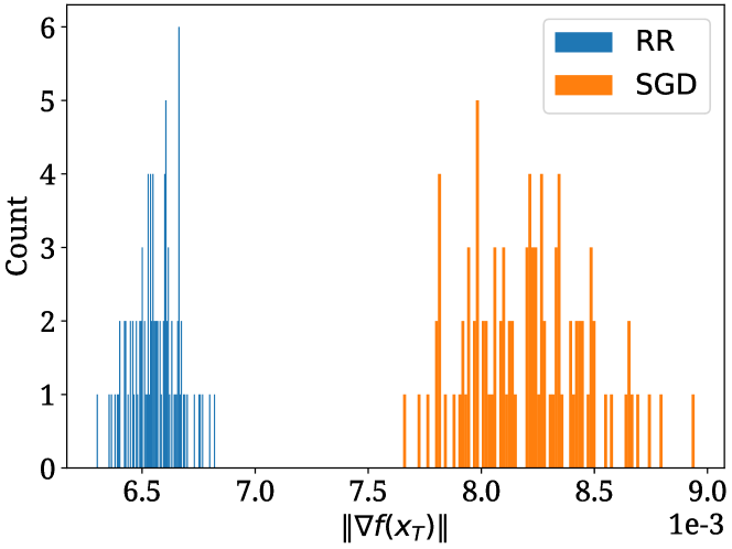
(a) Gradient norm statistics for the last iterate over 100 independent runs.

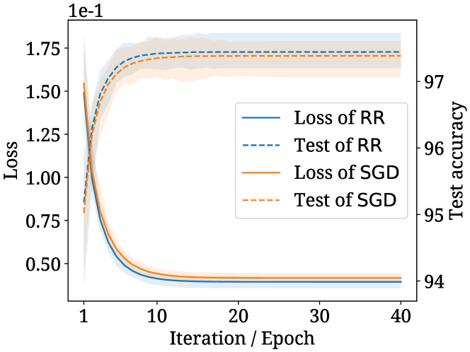
(b) Training loss and test accuracy of ${\sf RR}$ and SGD over 100 independent runs.

Figure 2: Comparison of performance between ${\sf RR}$ and SGD.

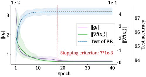
Figure 3: Evolution of $\|g_{t}\|$, $\|\nabla f(x_{t})\|$, and test accuracy of ${\sf RR}$.

We display the gradient norm statistics for the last iterate in both algorithms in Figure 2(a). It can observed that ${\sf RR}$ not only tends to yield a smaller gradient norm of the last iterate, but also exhibits a superior concentration property. This empirical observation corroborates our theoretical findings that the gradient norm in ${\sf RR}$ converges with high probability (see Theorem 2.7). In Figure 2(b), we show the training loss and test accuracy of ${\sf RR}$ and SGD. We can conclude that ${\sf RR}$ provides a slightly smaller training loss and demonstrates a slightly superior test accuracy.

In addition, we conduct experiments to study the stopping criterion $\|g_{t}\|\leq\eta\varepsilon$ defined in (3.1). The result is displayed in Figure 3. We observed that $\|g_{t}\|$ finally aligns with $\|\nabla f(x_{t})\|$ after $20$ iterations (epochs), corroborating our Theorem 3.4. It is also demonstrated that $\|g_{t}\|$ decreases along with the iteration index $t$. Upon setting the stopping criterion in (3.1) to $\|g_{t}\|\leq 7\times 10^{-3}$, the training process completes around the $17$th iteration (epoch), yielding a converged test accuracy. This suggests that $\|g_{t}\|$ is a practical measure that can be used as a stopping criterion.

Finally, we also conduct experiments on ${\sf p}\text{-}{\sf RR}$. The performance of ${\sf p}\text{-}{\sf RR}$ closely mirrors that of ${\sf RR}$, likely due to the fact that ${\sf RR}$ will not be trapped by strict saddle points in practical implementations. Therefore, we choose to omit these displays.

6 Conclusion and Discussions

In this work, we established a series of high probability guarantees for ${\sf RR}$. In particular, we derived a high probability sample complexity guarantee for identifying a stationary point by studying the concentration property of the sampling scheme in ${\sf RR}$. Furthermore, we proposed a stopping criterion for ${\sf RR}$, which gives rise to ${\sf RR}\text{-}{\sf sc}$. Such a stopping criterion terminates the method after a finite number of iterations and returns an iterate with its gradient below $\varepsilon$ with high probability. Lastly, we designed a perturbed random reshuffling method (${\sf p}\text{-}{\sf RR}$) for escaping strict saddle points. High probability convergence result to a second-order stationary point was established for ${\sf p}\text{-}{\sf RR}$, without making any sub-Gaussian tail-type assumptions on the stochastic gradient errors.

The dependence on $n$ in (2.5) is caused by bounding the random variable in (2.7) using variance. While it does not affect our complexity, improving $n$ to $i$ (if possible) could be insightful. Additionally, our current second-order complexity guarantee does not match the one for finding a stationary point, which is a natural direction for further improvement. We leave these areas for future exploration.

References

• [1] Dimitriย P Bertsekas. Incremental proximal methods for large scale convex optimization. Mathematical Programming, 129(2):163โ€“195, 2011.
• [2] Lรฉon Bottou. Curiously fast convergence of some stochastic gradient descent algorithms. In Proceedings of the symposium on learning and data science, volumeย 8, pages 2624โ€“2633, 2009.
• [3] Lรฉon Bottou. Stochastic gradient descent tricks. In Neural Networks: Tricks of the Trade, pages 421โ€“436. Springer, 2012.
• [4] Lรฉon Bottou, Frankย E Curtis, and Jorge Nocedal. Optimization methods for large-scale machine learning. SIAM Review, 60(2):223โ€“311, 2018.
• [5] Jaeyoung Cha, Jaewook Lee, and Chulhee Yun. Tighter lower bounds for shuffling sgd: Random permutations and beyond. International Conference on Machine Learning, 2023.
• [6] Yuejie Chi, Yueย M Lu, and Yuxin Chen. Nonconvex optimization meets low-rank matrix factorization: An overview. IEEE Transactions on Signal Processing, 67(20):5239โ€“5269, 2019.
• [7] Ashok Cutkosky and Harsh Mehta. High-probability bounds for non-convex stochastic optimization with heavy tails. Adv. in Neural Information Processing Systems, 34:4883โ€“4895, 2021.
• [8] Rong Ge, Furong Huang, Chi Jin, and Yang Yuan. Escaping from saddle pointsโ€”online stochastic gradient for tensor decomposition. In Conference on Learning Theory, pages 797โ€“842, 2015.
• [9] Rong Ge, Chi Jin, and Yiย Zheng. No spurious local minima in nonconvex low rank problems: A unified geometric analysis. In International Conference on Machine Learning, 2017.
• [10] Saeed Ghadimi and Guanghui Lan. Stochastic first- and zeroth-order methods for nonconvex stochastic programming. SIAM Journal on Optimization, 2013.
• [11] Eduard Gorbunov, Marina Danilova, and Alexander Gasnikov. Stochastic optimization with heavy-tailed noise via accelerated gradient clipping. Adv. in Neural Info. Processing Systems, 2020.
• [12] David Gross and Vincent Nesme. Note on sampling without replacing from a finite collection of matrices. arXiv preprint arXiv:1001.2738, 2010.
• [13] Mย Gรผrbรผzbalaban, Aย Ozdaglar, and Pabloย A Parrilo. Convergence rate of incremental gradient and incremental Newton methods. SIAM Journal on Optimization, 29(4):2542โ€“2565, 2019.
• [14] Mert Gรผrbรผzbalaban, Asu Ozdaglar, and PAย Parrilo. Why random reshuffling beats stochastic gradient descent. Mathematical Programming, 186(1-2):49โ€“84, 2021.
• [15] Jeff Haochen and Suvrit Sra. Random shuffling beats SGD after finite epochs. In International Conference on Machine Learning, pages 2624โ€“2633, 2019.
• [16] Nicholas J.ย A. Harvey, Christopher Liaw, Y.ย Plan, and Sikander Randhawa. Tight analyses for non-smooth stochastic gradient descent. Annual Conference Computational Learning Theory, 2018.
• [17] Wassily Hoeffding. Probability inequalities for sums of bounded random variables. Journal of the American Statistical Association, 58(301):13โ€“30, 1963.
• [18] Xinmeng Huang, Kun Yuan, Xianghui Mao, and Wotao Yin. An improved analysis and rates for variance reduction under without-replacement sampling orders. Advances in Neural Information Processing Systems, 34, 2021.
• [19] Chi Jin, Rong Ge, Praneeth Netrapalli, Shamย M Kakade, and Michaelย I Jordan. How to escape saddle points efficiently. In International conference on machine learning, pages 1724โ€“1732, 2017.
• [20] Chi Jin, Praneeth Netrapalli, Rong Ge, Shamย M Kakade, and Michaelย I Jordan. On nonconvex optimization for machine learning: Gradients, stochasticity, and saddle points. Journal of the ACM, 68(2):1โ€“29, 2021.
• [21] Ahmed Khaled and Peter Richtรกrik. Better theory for sgd in the nonconvex world. Transactions on Machine Learning Research, 2022.
• [22] Hunter Lang, Lin Xiao, and Pengchuan Zhang. Using statistics to automate stochastic optimization. In Advances in Neural Information Processing Systems, 2019.
• [23] Xiao Li and Andre Milzarek. A unified convergence theorem for stochastic optimization methods. In Advances in Neural Information Processing Systems, volumeย 35, pages 33107โ€“33119, 2022.
• [24] Xiao Li, Andre Milzarek, and Junwen Qiu. Convergence of random reshuffling under the kurdyka-ล‚ojasiewicz inequality. SIAM Journal on Optimization, 33(2):1092โ€“1120, 2023.
• [25] Yucheng Lu, Wentao Guo, and Christopherย De Sa. GraB: Finding provably better data permutations than random reshuffling. Neural Information Processing Systems, 2022.
• [26] Grigory Malinovsky, Alibek Sailanbayev, and Peter Richtรกrik. Random reshuffling with variance reduction: New analysis and better rates. Conference on Uncertainty in Arti. Intell., 2021.
• [27] Konstantin Mishchenko, Ahmed Khaled, and Peter Richtรกrik. Random reshuffling: Simple analysis with vast improvements. Advances in Neural Information Processing Systems, 2020.
• [28] Aryan Mokhtari, Mert Gรผrbรผzbalaban, and Alejandro Ribeiro. Surpassing gradient descent provably: A cyclic incremental method with linear convergence rate. SIAM Journal on Optimization, 28(2):1420โ€“1447, 2018.
• [29] Angelia Nediฤ‡ and Dimitriย P Bertsekas. Incremental subgradient methods for nondifferentiable optimization. SIAM Journal on Optimization, 12(1):109โ€“138, 2001.
• [30] Yurii Nesterov. Introductory lectures on convex optimization: A basic course, volumeย 87. Springer Science & Business Media, 2003.
• [31] Lamย M Nguyen, Quoc Tran-Dinh, Dzungย T Phan, Phuongย Ha Nguyen, and Marten Vanย Dijk. A unified convergence analysis for shuffling-type gradient methods. The Journal of Machine Learning Research, 22(1):9397โ€“9440, 2021.
• [32] Vivak Patel. Stopping criteria for, and strong convergence of, stochastic gradient descent on Bottou-Curtis-Nocedal functions. Mathematical Programming, 195(1-2):693โ€“734, 2022.
• [33] Shashank Rajput, Anant Gupta, and Dimitris Papailiopoulos. Closing the convergence gap of SGD without replacement. International Conference On Machine Learning, 2020.
• [34] Benjamin Recht and Christopher Rรฉ. Parallel stochastic gradient algorithms for large-scale matrix completion. Mathematical Programming Computation, 5(2):201โ€“226, 2013.
• [35] Herbert Robbins and Sutton Monro. A stochastic approximation method. The annals of mathematical statistics, pages 400โ€“407, 1951.
• [36] Itay Safran and Ohad Shamir. How good is SGD with random shuffling? In Conference on Learning Theory, volume 125, pages 3250โ€“3284, 2020.
• [37] Ruo-Yu Sun. Optimization for deep learning: An overview. Journal of the Operations Research Society of China, 8(2):249โ€“294, 2020.
• [38] Joelย A. Tropp. An introduction to matrix concentration inequalities. Foundations and Trendsยฎ in Machine Learning, 8(1-2):1โ€“230, 2015.
• [39] George Yin. A stopping rule for the Robbins-Monro method. Journal of Optimization Theory and Applications, 67(1):151โ€“173, 1990.
• [40] Chulhee Yun, Shashank Rajput, and Suvrit Sra. Minibatch vs local SGD with shuffling: Tight convergence bounds and beyond. In International Conference on Learning Representations, 2022.
• [41] Jingzhao Zhang, Saiย Praneeth Karimireddy, Andreas Veit, Seungyeon Kim, Sashank Reddi, Sanjiv Kumar, and Suvrit Sra. Why are adaptive methods good for attention models? Adv. in Neu. Info. Process. Systems, 2020.