Log-periodic oscillations as real-time signatures
of hierarchical dynamics in proteins

Abstract

The time-dependent relaxation of a dynamical system may exhibit a power-law behavior that is superimposed by log-periodic oscillations. Sornette [Phys. Rep. 297, 239 (1998)] showed that this behavior can be explained by a discrete scale invariance of the system, which is associated with discrete and equidistant timescales on a logarithmic scale. Examples include such diverse fields as financial crashes, random diffusion, and quantum topological materials. Recent time-resolved experiments and molecular dynamics simulations suggest that discrete scale invariance may also apply to hierarchical dynamics in proteins, where several fast local conformational changes are a prerequisite for a slow global transition to occur. Employing entropy-based timescale analysis and Markov state modeling to a simple one-dimensional hierarchical model and biomolecular simulation data, it is found that hierarchical systems quite generally give rise to logarithmically spaced discrete timescales. By introducing a one-dimensional reaction coordinate that collectively accounts for the hierarchically coupled degrees of freedom, the free energy landscape exhibits a characteristic staircase shape with two metastable end states, which causes the log-periodic time evolution of the system. The period of the log-oscillations reflects the effective roughness of the energy landscape, and can in simple cases be interpreted in terms of the barriers of the staircase landscape.

I Introduction

Complex systems such as biomolecules exhibit motions on many timescales, ranging from sub-picosecond vibrations to global conformational rearrangements requiring seconds.Hu16 ; Lindorff-Larsen16 Rather than being uncoupled as assumed in normal mode theory,Cui06 these molecular motions may interact in a nonlinear and cooperative manner, such that fast fluctuations are a prerequisite of rare transitions.Palmer84 ; Buchenberg15 The basic concept of such a hierarchical coupling of multiscale motions is often illustrated by a one-dimensional (1D) model of the free energy landscape, which represents the dynamics on different timescales by various tiers of the energy.Frauenfelder91 ; Dill97 ; Henzler-Wildman07a ; Milanesi12 As an example, Fig. 1a displays a free energy landscape showing three tiers A, B and C, which are associated with specific processes happening on $\mu$s, ns and ps timescales, respectively. Because the system needs to cross the barriers of tier C to reach the barriers of tier B and tier A, the hierarchical model give a simple explanation of the mechanistic coupling between fast and slow motions.

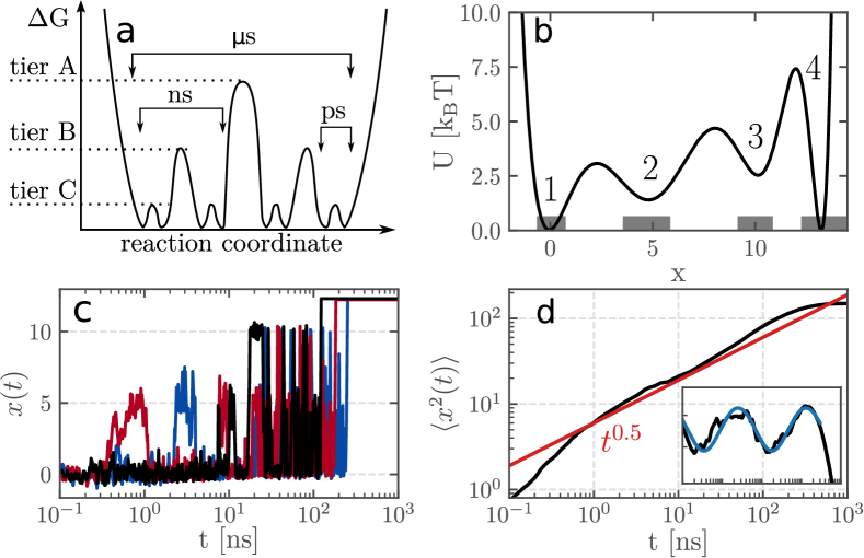
Figure 1: Hierarchical dynamics in proteins. (a) Scheme of a hierarchical free energy landscape that represents dynamical processes on $\mu$s, ns and ps timescales by tiers A, B and C. (b) One-dimensional (1D) model potential $U(x)$, consisting of states ${\bf 1}-{\bf 4}$ connected via energy barriers of similar height. Gray regions at the bottom define cores of the states used in Markov state modeling. (c) Time evolution $x(t)$ of three sample trajectories starting at $x=0$, which need several attempts to gradually climb over consecutive energy barriers. (d) Averaging over many trajectories, the resulting mean squared displacement ($\langle x^{2}(t)\rangle$, in black) shows a power-law behavior ($\propto t^{0.5}$, in red) that is superimposed by log-periodic oscillations. The enclosure shows a fit (blue) of the oscillatory residual $R(t)$ defined in Eq. (21).

While the concept of a hierarchical energy landscape is appealing, the microscopic nature of the tiers and the associated couplings between them is not well understood. In principle, such mechanisms can be inferred directly from all-atom molecular dynamics (MD) simulations, which reveal the local structural changes that are required for a global conformational rearrangement.Maisuradze13 For example, by considering the left- to right-handed transitions of the helical peptide Aib₉, Buchenberg et al.Buchenberg15 showed that these global transitions (occurring on a $0.1\mu$s timescale) first require conformational transitions of individual residues (which take about 1 ns), which in turn require the opening and closing of structure-stabilizing hydrogen bonds (occurring within tens of ps). Since the rates of these three processes were found to exhibit a similar temperature behavior, they concluded that the heights of the corresponding energy barriers must be similar, which appears to be in contrast to the energy landscape shown in Fig. 1a.

Represented by a one-dimensional (1D) model, these findings leads to a staircase-like energy landscape $U(x)$ depicted in Fig. 1b. The model consists of four states that are separated by three energy barriers, whose similar height ($\sim 3\,k_{\rm B}T$) corresponds roughly to the energy required to break a hydrogen bond. In this way, $x$ could be considered as collective coordinate constructed from the sum of three hydrogen bond distances.Lickert21 Assuming that the system starts at time $t=0$ in state 1, it evolves via intermediate states 2 and 3, and finally reaches the second low-energy state 4. Figure 1c shows three sample trajectories $x(t)$ of the model, see Methods for details. Starting in state 1, the system will initially cross the first barrier to state 2, but then typically fall back to 1 due to the high back-rate of the model. After some attempts, a rare fluctuation may drive the system over the second barrier to reach state 3, until after many more attempts the system will eventually reach the final state 4. Using a logarithmic representation of time, this gradual climbing over similar energy barriers manifest itself in apparent log-oscillations of $x(t)$.

To explain these findings, we assume that the mean transition time over the first barrier (with energy $E_{b}$) is given by $\tau_{1\rightarrow 2}=\tau_{0}e^{-\beta E_{b}}$, where $\beta=1/k_{\rm B}T$ denotes the inverse temperature. Since all barriers are similar, we roughly estimate that transitions over the first two barriers take about $\tau_{1\rightarrow 3}=\tau_{0}e^{-2\beta E_{b}}$, and analogously $\tau_{1\rightarrow 4}=\tau_{0}e^{-3\beta E_{b}}$. This leads to the relation

$$\log\tau_{1\rightarrow n+1}-\log\tau_{1\rightarrow n}=\beta E_{b}\log{\rm e},$$ (1)

where $\log{\rm e}=\log x/\ln x$ denotes the decadic logarithm of Euler’s number. It states that the system exhibits discrete and equidistant timescales on a logarithmic scale, which explain the log-periodic oscillations of $x(t)$.

Log-periodic oscillations have been found in such diverse fields as the diffusion on random lattices, Bernasconi82 ; Klafter91 in dielectric relaxation Khamzin13 and the magnetoresistance of ultraquantum topological materials, Wang18c as well as in large-scale phenomena such as earthquakes Sornette95 and financial crashes. Johansen98 ; Geraskin13 Following Sornette,Sornette98 they arise as a consequence of a discrete scale invariance, meaning that the scale invariance exists only for transformations $t\rightarrow\lambda t$ with discrete values of the scaling parameter $\lambda$, that is, $\lambda=\lambda_{n}=\kappa^{n}$. These relations results directly in Eq. (1), when we set $\kappa=e^{\beta E_{b}}$ and $\lambda_{n}=\tau_{1\rightarrow n}/\tau_{0}$. Performing an ensemble average over many trajectories starting at $x=0$, the theory predicts for the resulting mean position $\langle x(t)\rangle$ and mean squared displacement $\langle x^{2}(t)\rangle$ a power-law behavior superimposed by a weak log-oscillatory pattern.Sornette98 Showing $\langle x^{2}(t)\rangle$ together with the associated power law $t^{0.5}$ and its residual oscillatory part, Fig. 1d reveals that this is indeed the case for the 1D model. While power laws are the hallmark of scale-invariant and self-similar systems, the emergence of log-periodic oscillations require the discreetness of the underlying timescales.

Hence we have shown that the hierarchical structure of the 1D model approximately obeys the condition of discrete scale invariance and thus gives rise to log-periodic oscillations. While this condition is indeed satisfied by various hierarchical models, Bernasconi82 ; Sornette98 ; Metzler99 ; Lickert21 it is less clear whether it is also obeyed by the free energy tiers of a real protein. If so, log-periodic oscillations should be observable in MD simulations as well as in time-resolved experiments. This might be indeed the case. For example, Hamm and coworkers designed photoswitchable proteins that initially trigger a local photoinduced conformational change, whose propagation through the protein can be monitored via transient infrared spectroscopy. Buchli13 ; Bozovic20 ; Bozovic20a ; Bozovic21 ; Bozovic22 Their experiments on various PDZ domains exhibited strongly nonlinear dynamics on timescales from picoseconds to tens of microseconds. Accompanying MD studies of the nonequilibrium conformational dynamics reproduced these findings and revealed a quite complex structural reorganization of the protein Nguyen06b ; Buchenberg14 ; Buchenberg17 ; Ali22 In particular, the time traces of both experiment and MD revealed overshootings, which may indicate log-periodic oscillations.Stock18

In this work we wish to explore the applicability and relevance of discrete scale invariance for the modeling and understanding of hierarchical dynamics in proteins. To this end, we first consider the above 1D system as a proof-of-principle model. As we in general rely on experimental or simulation results, we adopt a data-driven approach that does not use information on the underlying theoretical formulation of the model. Considering the time evolution of the system as input data, we aim to construct a dynamical model of the underlying dynamics. To focus first on ensemble-averaged data, we perform a timescale analysis using a maximum entropy method. Stock18 ; Lorenz-Fonfria06 Employing furthermore single-molecule (i.e., single-trajectory) information, Berezhkovskii20 we can recover the free-energy landscape of the model and construct a Langevin equationLange06b ; Hegger09 ; Ayaz21 or a Markov state model. Bowman13a ; Wang17a ; Noe19 The analyses are shown to result in a multiexponential response function with discrete timescales, giving rise to log-periodic oscillations.

To test if the concepts are applicable to real data, we revisit the above mentioned hierarchical dynamics of the achiral peptide helix Aib₉.Buchenberg15 As the process evolves in a high-dimensional coordinate space, we first need to define collective variables that account for the hierarchically coupled degrees of freedom. Employing nonequilibrium MD simulations, we again use a timescale analysis and construct a Markov state model to identify the timescales of the process. We study the conditions under which log-periodic oscillations can be observed for Aib₉, and close with a discussion what aspects of hierarchical dynamics may be learned from these phenomena.

II Theory

As explained above, we wish to analyze a time series given from a nonequilibrium experiment or MD simulation, using three theoretical formulations: Maximum entropy timescale analysis, Lorenz-Fonfria06 Markov state modeling, Bowman13a ; Wang17a ; Noe19 and discrete scale invariance.Sornette98 Moreover, we discuss if the same effects can be also observed under equilibrium conditions.

II.1 Timescale analysis

The time evolution of a relaxation process can be described by a multiexponential response function

$$S(t)=s_{0}-\sum_{k=1,K}s_{k}\,e^{-t/\widehat{\tau}_{k}},$$ (2)

where $S(t)$ is the considered observable of the system (e.g., $S\!=\!\langle x\rangle$ for the 1D system), which was prepared at $t\!=\!0$ in a nonequilibrium initial state (e.g., state 1 in Fig. 1b). The first term with $\widehat{\tau}_{0}=\infty$ gives the offset $s_{0}$, and the time constants $\widehat{\tau}_{k}$ ($k\geq 1$) with amplitudes $s_{k}$ are given in decreasing order. To analyze the timescales inherent to a given time series $S(t)$, we determine the timescale spectrum $s(\widehat{\tau}_{k})\equiv s_{k}$. To this end, we choose the time constants to be equally distributed on a logarithmic scale (typically 10 terms per decade) and fit the corresponding amplitudes $s_{k}$ to the data. When we assume that $S(t)$ is monotonic increasing, we can choose $s_{k}\geq 0$. The local maxima of the spectrum

$$\tau_{n}=\{\tau,\;s(\tau)={\rm max}\}$$ (3)

are referred to as ’main timescales’ of the process.

Equation (2) corresponds to an inverse Laplace transformation, which is an ill-posed problem, because the included exponential functions are not orthogonal to each other. To render the fitting algorithm stable, we therefore introduce an entropy-based regularization factor $S_{\rm ent}$ that enforces a smooth spectrum of the amplitudes $s_{k}$. This is achieved by minimizing the weighted sum $\chi^{2}-\lambda_{\rm reg}S_{\rm ent}$ of this penalty function together with the usual root mean square deviation $\chi^{2}$ of the fit function to the data. Lorenz-Fonfria06 The regularization parameter $\lambda_{\rm reg}$ controls whether the model is over- or underfitted. $\lambda_{\rm reg}$ can be estimated via various criteria; see the Supplementary Material for details (Fig. S1).

II.2 Markov state modeling

If the free-energy landscape $\Delta G(x)$ of the system is known (e.g., from single-trajectories), we may construct a Markov state model (MSM), Bowman13a ; Wang17a ; Noe19 which describes the dynamics in terms of memory-less jumps between $N$ metastable conformational states of the system. Assuming a timescale separation between fast intrastate fluctuations and rarely occurring interstate transitions (i.e., the Markov approximation), the dynamics of the system is completely determined by the transition matrix $T(\tau_{\text{lag}})$ containing the probabilities $T_{ij}$ that the system jumps from state $j$ to $i$ within lag time $\tau_{\text{lag}}$. Denoting the state vector at time $t$ by $\boldsymbol{p}(t)=(p_{1},\ldots,p_{N})^{T}$ with state probabilities $p_{i}$, the time evolution of the MSM is given by

$$\boldsymbol{p}(t\!=\!k\tau_{\rm lag})=T^{k}(\tau_{\rm lag})\boldsymbol{p}(0).$$ (4)

Upon diagonalizing the transition matrix $T$, we obtain its left/right eigenvectors $\boldsymbol{\psi}^{\rm l}_{n}$/$\boldsymbol{\psi}^{\rm r}_{n}$ and eigenvalues $\mu_{n}$. The latter yield the implied timescales

$$t_{n}=-\tau_{\text{lag}}/\ln\mu_{n}$$ (5)

of the system, which correspond to experimentally measurable quantities that account for the exponential decay $e^{-t/t_{n}}$ associated with eigenvector $\boldsymbol{\psi}_{n}$. Performing an eigendecomposition of the transition matrix, the time evolution can be written as a sum of decay factors multiplied with the overlap of the eigenvectors with the initial state, Noe11

$$\boldsymbol{p}(t\!=\!k\tau_{\rm lag})=\sum_{n=0,N-1}\langle\boldsymbol{\psi}_{n}^{\rm r}|\boldsymbol{p}(0)\rangle\,e^{-t/t_{n}}\,\boldsymbol{\psi}_{n}^{\rm l}\,,$$ (6)

where $\boldsymbol{\psi}_{0}$ accounts for the equilibrium distribution associated with $t_{0}=\infty$. Assuming that the observable of interest, $S$, adopts in state i the mean value $\langle s\rangle_{i}$, we obtain again a multiexponential representation of the time evolution of the observable, i.e.,

$$S(t)=\sum_{i=0,N-1}\langle s\rangle_{i}\,p_{i}(t)=\sum_{n=0,N-1}\hat{s}_{n}\,e^{-t/t_{n}}$$ (7)

with $\hat{s}_{n}=\sum_{i}\langle s\rangle_{i}\langle{\bf i}|\boldsymbol{\psi_{n}^{\rm l}}\rangle\langle\boldsymbol{\psi}_{n}^{\rm r}|\boldsymbol{p}(0)\rangle$.Noe11 While the MSM description of $S(t)$ has the same functional form as the timescale analysis expression in Eq. (2), we note that the sum now runs over the $N$ implied timescales $t_{n}$ of the $N$-state system.

II.3 Discrete scale invariance

Following Sornette,Sornette98 we summarize the basic ideas of discrete scale invariance, which are relevant in the further discussion. A time-dependent observable $S(t)$ is said to be scale invariant under the transformation $t\rightarrow\lambda t$, if

$$S(t)=\mu(\lambda)S(\lambda t).$$ (8)

For notational convenience, the time $t$ is given in dimensionless units. The solution of this equation follows a power law with exponent $\widetilde{\alpha}$,

$$S(t)=ct^{\widetilde{\alpha}},$$ (9)

which can be verified by insertion. For example, the diffusion on a flat energy landscape ($U(x)=const.$) is scale invariant, that is, it looks the same on all time and length scales.

While this is in general not true for diffusion on a position-dependent potential $U(x)$, a weaker condition, discrete scale invariance, may apply if Eq. (8) holds at least for discrete values of the scaling parameter $\lambda$, that is,

$$\lambda=\lambda_{n}=\kappa^{n}\quad(n\in\mathbb{N}),$$ (10)

where $\kappa$ is the fundamental scaling ratio. This condition reflects a symmetry of the problem, such as a lattice potential or the above considered hierarchical landscape. Inserting Eq. (10) in (8), we obtain

$$\mu\lambda^{\widetilde{\alpha}}=1=e^{\mathrm{i}2\pi m}\quad(m\in\mathbb{Z}),$$ (11)

where the second equation indicates that the exponent is in general complex valued and can be written as

$$\widetilde{\alpha}=-\frac{\ln\mu}{\ln\lambda}+\mathrm{i}\frac{2\pi m}{\ln\lambda}\equiv\alpha+\mathrm{i}\omega.$$ (12)

Using $t^{\mathrm{i}\omega}=e^{\mathrm{i}\omega\ln t}$ and assuming that $S=\mathrm{Re}\,S$, we obtain

$$S(t)=ct^{\alpha}\cos(\omega\ln t),$$ (13)

indicating that $S(t)$ exhibits log-periodic oscillations. Assuming discrete scale invariance [Eq. (10)], the frequency $\omega$ depends only on the fundamental scaling ratio $\kappa$,

$$\omega=\frac{m2\pi}{n\ln\kappa}=\frac{2\pi}{\ln\kappa}\;,$$ (14)

because $m$ is an arbitrary integer, which can be chosen as $m=n$. This is in contrast to the case of general scale invariance (where $\lambda$ can take an arbitrary value), which results in a frequency $\omega\propto 1/\ln\lambda$ that is not constant. Hence, the existence of the log-oscillations rests on the existence of discrete scaling parameters $\lambda_{n}=\kappa^{n}$.

Let us apply the above theory to our hierarchical model introduced in Fig. 1b. Showing consecutive barriers of similar height $\beta E_{b}$, the system is expected to approximately exhibit transition times, $\tau_{1\rightarrow n}=\tau_{0}e^{(n\!-\!1)\beta E_{b}}$, that are discrete and equidistant on a logarithmic scale, see Eq. (1). Associating these timescales with the scaling parameter via

$$\lambda_{n}=e^{n\beta E_{b}},$$ (15)

we obtain for the fundamental scaling ratio

$$\kappa=e^{\beta E_{b}},$$ (16)

which is inverse proportional to the probability to cross single barrier. Introducing $\tau_{\rm log}=\log{\rm e}\;2\pi/\omega$, we find from Eqs. (14) and (16)

$$\tau_{\rm log}=\beta E_{b}\log{\rm e}$$ (17)

(with $\log{\rm e}\approx 0.43$), stating that the period of the oscillations in decadic log time directly reflects the average barrier height of the hierarchical energy landscape.

When we consider a time trace $S(t)$ obtained from an experiment or MD simulation, we generally do not know the underlying energy landscape and the corresponding transition times. Nonetheless, we may perform a timescale analysis [Eq. (3)] to obtain the main exponential timescales $\tau_{1}\geq\tau_{2}\geq\tau_{3}\ldots$. In direct analogy to Eq. (1), the existence of log-oscillations then requires that these timescales are equally spaced by their period $\tau_{\rm log}$,

$$\log\tau_{n}-\log\tau_{n+1}=\tau_{\rm log}\,.$$ (18)

Note that this condition is certainly fulfilled in the common case that only two main timescales exist, $\tau_{1}$ and $\tau_{2}$. When we associate $\tau_{2}$ with the crossing of the first barrier $\beta E_{1}$ and $\tau_{1}$ with the timescale of the barrier $\beta E_{\rm tot}$ of the overall transition, we obtain from our simple rate-theory consideration

$$\tau_{\rm log}=\beta(E_{\rm tot}-E_{1})\log{\rm e}$$ (19)

stating that the log-period reflects the energy difference of the overall and initial barriers.

Since the barrier heights of a 1D energy landscape do not necessarily reflect the true reaction rates of a multidimensional system,Altis08 in general we cannot directly associate $\tau_{\rm log}$ with specific barriers of the system. Rather the energy $\Delta E=\tau_{\rm log}/(\beta\log{\rm e})$ reflects an overall roughness of the energy landscape, which gives rise to an effective diffusion coefficient or intramolecular friction of the process. Milanesi12 ; Zwanzig88 ; Schulz12 ; Echeverria14

II.4 Modeling log-periodic power laws

To be able to fit given MD data to a log-periodic power law $S(t)$, we generalize Eq. (13) to the functional form

$$S(t)=s_{a}+s_{b}t^{\alpha}+s_{c}t^{\alpha}\cos(\tfrac{2\pi}{\tau_{\rm log}}\log t+\varphi),$$ (20)

which introduces the amplitudes $s_{b}$ and $s_{c}$ and the phase $\varphi$ defining the oscillations, and the initial value $s_{a}$, which is chosen such that $S(t)>0$. To discuss the oscillations, we also consider the oscillatory residual, defined as

$$R(t)=(S(t)-s_{a})t^{-\alpha}.$$ (21)

It is instructive to study to what extent a simple multiexponential model $S(t)=\sum_{n}s_{n}\,e^{-t/\tau_{n}}$ with only two or three main timescales $\tau_{n}$ and associated amplitudes $s_{n}$ can give rise to the log-periodic power law in Eq. (20). To this end, Fig. S2 shows power-law fits for models with various choices of the timescales and amplitudes. Using two timescales that are more than one decade apart, i.e., $\log\tau_{1}-\log\tau_{2}\equiv\Delta_{12}\gtrsim 1$, we obtain two well-defined log-oscillations with $\tau_{\rm log}\approx\Delta_{12}$ for various choices of the amplitudes. On the other hand, if the timescales are too close to each other ($\Delta_{12}<1$), we effectively see only a single exponential term without log-oscillations. The scenario is similar for three timescales. If the timescale are roughly logarithmically equidistant and well separated, i.e., $\Delta_{12}\approx\Delta_{23}\gtrsim 1$, we obtain three well-defined log-oscillations. If two of the timescales are too close to each other, we find only two exponential terms and two log-oscillations.

II.5 Nonequilibrium vs. equilibrium conditions

In the discussion above, we have assumed nonequilibrium initial conditions, i.e., we initially prepared the system in a nonstationary state. This raises the question, if the same effects can be observed under equilibrium conditions. Assuming linear response conditions, for example, the nonequilibrium time evolution of the ensemble average $\langle x(t)\rangle$ is known to be closely related to the autocorrelation function

$$C(t)=\langle\delta x(t)\delta x(0)\rangle_{\rm eq}/\langle\delta x^{2}\rangle_{\rm eq},$$ (22)

where $\delta x=x\!-\!\langle x\rangle$ and $\langle\ldots\rangle$ denotes a time average over an equilibrium trajectory.Chandler87 In the nonequilibrium set-up considered in Fig. 1, however, we typically stop the experiment or simulation, once the system reaches the final state 4. In this way, we prevent the reverse reaction out of this state and the subsequent propagation of the system, which would occur under equilibrium conditions. The reverse reaction may introduce additional timescales that are not encountered in the forward reaction. Moreover, the nonequilibrium preparation results in well-defined initial conditions for the climb over the energy landscape, which may lead to an oscillatory behavior of the nonequilibrium ensemble average $\langle x(t)\rangle$. On the other hand, the averaging over an equilibrium trajectory may average over these oscillations.

III Discussion of the 1D model

III.1 Methods

Employing the 1D energy landscape $U(x)$ shown in Fig. 1b, simulations of the Langevin equation $m\ddot{x}(t)=-\frac{dU(x)}{dx}-\Gamma\dot{x}(t)+K\xi(t)$ were performed as described in Ref. Lickert21, . Specifically, we used a mass of $m\!=\!1$ u, constant friction ($\Gamma\!=\!130\,$kJ ps/mol) and noise amplitude ($K\!=\!25\,$kJ ps^1/2/mol), $\delta$-correlated Gaussian noise $\xi$ of zero mean, and a temperature $T\!=\!300\,$K. Collecting the data $x(t)$ every $\delta t=0.4\,$ps, we transformed to logarithmically spaced data for easier representation. To remove fast fluctuations, a Gaussian filter with a standard deviation of 6 frames is used. Starting at $x\!=\!0$, in total $N\!=\!3000$ trajectories were run until they reach state 4, i.e., for $x\!\geq\!12.3$. To calculate the mean position $\langle x(t)\rangle$, we performed an ensemble average over the $N$ trajectories, where the initial conditions of the individual trajectories were sampled from a Boltzmann velocity distribution. When we calculate the energy profile $\Delta{\cal G}(x)=-k_{\rm B}TP(x)$ from the resulting probability distribution $P(x)$, we consistently recover the potential energy $U(x)$. note1 Showing the convergence of the mean position $\langle x(t)\rangle$ with the sample size $N$, Figs. S3a,b reveal a smooth increase of $\langle x(t)\rangle$ for $N\gtrsim 10^{3}$, while for $N\lesssim 10^{2}$ we find additional high-frequency fluctuations as signatures of transitions of individual trajectories. This indicates that an incomplete sampling of the stochastic process can be easily misinterpreted as log-periodic oscillations of $\langle x(t)\rangle$.

As the 1D model in Fig. 1b is well characterized in terms of its states 1 to 4, we may construct a MSM, Bowman13a ; Wang17a ; Noe19 using our open-source Python package msmhelper.Nagel23a To this end, we first apply a Gaussian smoothing with a standard deviation of 2.4 ps to the individual trajectories $x(t)$.Nagel23b To avoid problems at the boundaries, we define the states via their cores Buchete08 ; Lemke16 ; Nagel19 (gray regions in Fig. 1b), that is, we assign states 1 to 4 to the $x$-regions [-0.6, 0.7], [3.6, 5.8], [9.2, 10.8], and $x\!\geq\!12.3$. Intermediate frames between these regions are assigned to the last populated state. The resulting state trajectories are then directly employed to calculate the transition matrix $T(\tau_{\text{lag}})$. Due to the coring procedure and since the underlying dynamics was generated by a Markovian Langevin equation, we expect the Markov approximation to hold well. As a consequence, the implied timescales of the 4-state model are constant already at lag time $\tau_{\text{lag}}=\delta t$, and the resulting Chapman-Kolmogorov equation (4) holds accurately, see Figs. S3c,d.

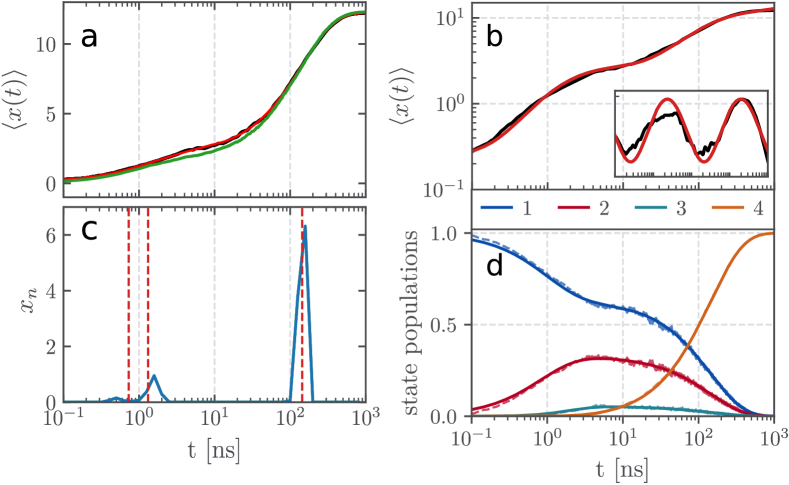
Figure 2: Analysis of the 1D model shown in Fig. 1b. (a) Mean position $\langle x(t)\rangle$, as obtained from (black) the Langevin simulations, (red) the fit of the timescale analysis [(Eq. (2)], and (green) the MSM [(Eq. (7)]. (b) Double-logarithmic representation of $\langle x(t)\rangle$ (black) together with the fit to Eq. (18) (red), showing the oscillatory residual $R(t)$ [Eq. (21)] in the enclosure. (c) Timescale spectrum [Eq. (2), in blue], compared to the implied timescales [Eq. (5), in red] of an MSM constructed from the Langevin data. (d) Time evolution of the state probabilities $p_{n}(t)$ of the MSM (thick lines) and the Langevin data (thin dashed lines).

III.2 Results

As detailed above, we run $N\!=\!3000$ Langevin simulations that start at time $t\!=\!0$ in state 1, and follow them until they reach the final state 4. Figures 2a,b show the time evolution of the resulting mean position $\langle x(t)\rangle$ in log-time and double-log representation, which reflects the gradual climb over the staircase-shaped energy landscape. To identify the timescales of this climb, we model the time evolution of $\langle x(t)\rangle$ by the multiexponential response function in Eq. (2), see Methods. The resulting maximum-entropy timescale spectrum ($\lambda_{\rm reg}\!=\!10$) shown in Fig. 2c exhibits two main timescales at $\tau_{1}\!=\!160$ ns and $\tau_{2}\!=\!1.6$ ns, and a rather weak signature at 0.5 ns. From the time evolution of the individual trajectories (Fig. 1c), we conclude that the short timescale reflects first attempts to cross the barrier to state 2, while the long timescale accounts for transitions to the final state 4.

From a data-driven view, the above timescale analysis requires only ensemble-averaged data [e.g., $\langle x(t)\rangle\propto\sum_{n}x_{n}(t)$]. If single-trajectory information [i.e., $x_{n}(t)$] is available,Berezhkovskii20 we can calculate the probability distribution along $x$ and thus recover the energy landscape $\Delta{\cal G}(x)=-k_{\rm B}T\ln P(x)$ of the model. By identifying the four metastable conformational states 1 to 4 of the system, we may then construct a MSM of the dynamics (see Methods). As expected for a simple 1D system, we find that the resulting implied timescales of the MSM, $t_{1}\!=\!145\,$ns, $t_{2}\!=\!1.3\,$ns and $t_{3}\!=\!0.7\,$ns, agree well with the main peaks of the timescale spectrum in Fig. 2c.

What is more, the MSM provides an explanation of these timescale in terms of the population flux between the states. Showing the time evolution of the population probabilities $p_{i}(t)$ of the four states, Fig. 2d reveals that the population of initial state 1 decays (within all three timescales $t_{3}$, $t_{2}$ and $t_{1}$) such that the intermediate states 2 and 3 are transiently populated (within $t_{3}$ and $t_{2}$), until the system relaxes in final state 4 (within $t_{1}$). When we compare the time evolution of the state populations obtained from the MSM to the Langevin results, we find excellent agreement. Moreover, the MSM calculation of the mean position $\langle x(t)\rangle$ via Eq. (7) matches perfectly the reference results (Fig. 2a).

Interestingly, we find that the fastest timescale $t_{3}\!=\!0.7\,$ns clearly shows up in the initial decay of $p_{1}(t)$ and the corresponding initial rise of $p_{2}(t)$, although it is hardly visible in the timescale analysis in Fig. 2c. This reflects the fact that the MSM exploits the structure of the energy landscape, while the timescale analysis only uses the evolution of the observable $\langle x(t)\rangle$, and thus depends considerably on the definition of the collective coordinate $x$.

We are now in a position to assess if the dynamics of the 1D problem fulfills the conditions of discrete scale invariance and therefore gives rise to a log-periodic power law. Figure 2c shows that both timescale analysis and MSM essentially yield only two timescales, $160$ ns and $1.6$ ns. (The third MSM timescale carries hardly any amplitude and can be omitted.) Alternatively, we may calculate the average transition times $\tau_{1\rightarrow n}$ to reach state $n$ after starting in state 1, yielding $\tau_{1\rightarrow 2}=2.6$ ns, $\tau_{1\rightarrow 3}=23$ ns and $\tau_{1\rightarrow 4}=147$ ns. As $\tau_{1\rightarrow 3}$ can be neglected (because state 3 is hardly populated, see Fig. 2d), we are again left with two times, which resemble closely the timescales determined by timescale analysis and the MSM. Because Eq. (18) is directly fulfilled if only two timescales exist, the 1D problem is expected to show typical phenomena associated with discrete scale invariance.

Using $\tau_{1}\!=\!160$ ns and $\tau_{2}\!=\!1.6$ ns, Eq. (18) predicts a log-periodic power law with an a period of $\tau_{\rm log}\!=\!2.0$. To test these predictions, we use the functional form in Eq. (20) and fit the Langevin data to a log-periodic power law. Figure 2b shows that we obtain a perfect fit, when we use $\tau_{\rm log}\!=\!1.92$ for the period, $\alpha\!=\!0.31$ for the exponent, and the coefficients $s_{a}\!=\!-0.5$, $s_{b}\!=\!1.7$, $s_{c}\!=\!-0.2$, and $\varphi\!=\!1.9$. The good agreement of theoretical [Eq. (18)] and fitted values for $\tau_{\rm log}$ is also reflected in the fact that the maxima of the log-periodic oscillation coincide well with the peaks of the timescale spectrum in Fig. 2c.

Moreover, Eq. (19) allows us to infer from the period $\tau_{\rm log}\!=\!2$ an effective roughness $\beta\Delta E\!=\!4.7$ of the underlying energy landscape. In the case of only two timescales, $\beta\Delta E$ can be interpreted as the energy difference of the the overall and initial barriers. Indeed the energy difference $\beta\Delta E=4.5$ obtained from the potential $U(x)$ in Fig. 1b agrees well with the theoretical prediction. When we employ the simple rate approximation of Eq. (15), we may also relate $\tau_{\rm log}$ to the average barrier height $\beta E_{b}$ of the hierarchical energy landscape via Eq. (17). In fact, $\beta E_{b}=3.8$ obtained from the potential $U(x)$ in Fig. 1b matches $\beta\Delta E\!=\!4.7$ at least qualitatively.

Apart from considering the mean $\langle x(t)\rangle$, it is interesting to discuss the mean squared displacement $\langle x^{2}(t)\rangle$, which accounts for the diffusional motion of the system. As shown in Fig. 1d, we obtain similar log-oscillations with $\tau_{\rm log}=1.72$ and an increase of the power-law exponent to $\alpha=0.5$. That is, the hierarchical dynamic of the 1D model manifest itself in subdiffusion, which reflects the roughness of the underlying energy landscape.Hu16 ; Milanesi12

So far, we have assumed a nonequilibrium preparation of the system in the initial state 1. To test if the same effects can be observed under equilibrium conditions, we run a $16\,\upmu$s-long equilibrium simulation of the 1D model and calculate the autocorrelation function $C(t)$ in Eq. (22). Figure S4 shows that $C(t)$ decays on the timescales $\tau_{1}=26\,$ns and $\tau_{2}=1.3\,$ns. While $\tau_{2}$ is similar to the implied timescale $t_{2}$ found in the nonequilibrium case, $\tau_{1}$ is significantly shorter than the nonequilibrium timescale $t_{1}=160\,$ns, which reflects the possibility of back-reaction from state 4. Moreover, we find that the equilibrium autocorrelation function shows no evidence of log-periodic oscillations. This indicates that the discrete scale invariance of the observable $\langle x(t)\rangle$ requires well-defined initial conditions (as given by a nonequilibrium preparation) as well as a well-defined end state, which prevent the averaging over the oscillations.

IV Hierarchical dynamics of a peptide helix

It is interesting to study to what extent the theoretical concepts established above for the 1D model can be transferred to the analysis of all-atom MD data. As a well-established model system, Buchenberg15 ; Perez18 ; Biswas18 ; Mehdi22 we consider the achiral peptide Aib₉ that undergoes complete left- to right-handed chiral transitions of the helix, see Fig. 3a.

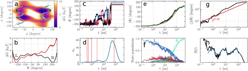
Figure 3: Hierarchical dynamics of the peptide helix Aib₉. (a) Structure of the left-handed and right-handed conformation of Aib₉, along with the Ramachandran plot $\Delta G(\phi,\psi)$, averaged over the five inner peptide residues. (b) Energy landscapes along the collective coordinate $\Phi$ [Eq. (23)], obtained from equilibrium MD simulationsBuchenberg15 (black) and from nonequilibrium trajectories that exhibit a single L$\rightarrow$R transition (red).note3 (c) Time evolution of three individual nonequilibrium trajectories $\Phi(t)$. (d) Timescale spectrum [Eq. (2), in blue], compared to the implied timescales [Eq. (5), in red] of an MSM constructed from the MD data. (e) Mean position $\langle\Phi(t)\rangle$, as obtained from (black) the nonequilibrium MD trajectories, (red) the fit of the timescale analysis [(Eq. (2)], and (green) the MSM [(Eq. (7)]. (f) Time evolution of the state probabilities $p_{n}(t)$ of the MSM. (g) Double-logarithmic representation of $\langle\Delta\Phi(t)\rangle=\langle\Phi(t)\rangle+255^{\circ}$ together with the associated power law $t^{0.46}$ and (h) the residual oscillatory part $R(t)$ [Eq. (21)].

IV.1 Model and methods

Buchenberg et al.Buchenberg15 performed extensive MD simulations of Aib₉ (H₃C-CO-(NH-C_α(CH₃)₂-CO)₉-CH₃), using the GROMACS program suite GROMACS05 with the GROMOS96 43a1 force fieldGROMOS96 and explicit chloroform solvent.Tironi94 Here we use eight of their MD trajectories at 320 K of each $2\ \mu$s length, using a time step $\Delta t=$ 1 ps. The resulting Ramachandran plot $\Delta G(\phi_{i},\psi_{i})$ along the backbone dihedral angles $(\phi_{i},\psi_{i})$ of the five inner peptide residues ($i=3,\ldots,7$) reveals a point symmetry with respect to (0,0), which shows that Aib₉ indeed samples both left-handed ($\phi_{i}\geq 0$) and right-handed ($\phi_{i}\leq 0$) conformations with similar probability (Fig. 3a). The corresponding two local conformational states l at $\approx$ (-50^∘, -45^∘) and r at $(50^{\circ},45^{\circ})$ correspond to a right- and left-handed helix, respectively.note3 The ring-shaped free energy landscape $\Delta G$ reveals that left- to right-handed transitions l$\leftrightarrow$r of a single residue along dihedral angle $\phi_{i}$ first requires a transition along dihedral angle $\psi$, which occurs about 10 times faster than l$\leftrightarrow$r transitions occurring on a 1 ns timescale. On the other hand, left- to right-handed chiral transitions of the entire helix, L$\leftrightarrow$R, requires individual l$\leftrightarrow$r transition of all residues, which occur on a 100 ns timescale.

In the following, we focus on this last tier of the hierarchical dynamics and study the L$\rightarrow$R transition, represented by the sum of the $\phi_{i}$ angles of the five inner residues,

$$\Phi=\sum_{i=3,7}\phi_{i}.$$ (23)

It was shown in Ref. Buchenberg15, that $\Phi$ is equivalent to the first component of a principal component analysis of all backbone dihedral angles. Riccardi09 Figure 3b shows the resulting free energy landscape $\Delta G(\Phi)$ obtained from the equilibrium MD simulations.note3 Adopting a product-state notation of the five inner residues, we note that the two main minima L = (lllll) and R = (rrrrr), are connected by four intermediate states with an increasing number of r-residues, e.g., (rllll), (rrlll,) (rrrll) and (rrrrl). As discussed elsewhere,Biswas18 the free energy difference ($\sim 1k_{\rm B}T$) between the states L and R is not due to incomplete sampling but is caused by an inaccuracy of the force field parameterization of Aib₉, which is not of interest here.

As discussed in Sec. II.5, the observation of log-periodic oscillations along $\Phi$ requires a nonequilibrium preparation and monitoring of the system (rather than equilibrium simulations that average over these oscillations). To this end, we extracted all L$\rightarrow$R transitions occurring during the $8\times 2\ \mu$s MD simulations (see the Supplementary Material for details). Starting when the system enters state L, monitoring the transition to state R, and ending when it reaches R, we thus obtain 63 independent nonequilibrium trajectories, which are used in the subsequent analysis. Calculating the probability distribution $P(\Phi)$ from these trajectories, the resulting energy landscape $\Delta{\cal G}(\Phi)=-k_{\rm B}TP(\Phi)$ is shown in Fig. 3b. Since each state along $\Delta{\cal G}(\Phi)$ serves as prerequisite for the overall L$\rightarrow$R transition, the energy landscape shows again the typical staircase shape, quite similar as anticipated by the 1D model. For Aib₉, the first and last barriers have a height of $\sim 1.7$ and $2.4\,k_{\rm B}T$, the three intermediate barriers of $\sim 0.8\,k_{\rm B}T$. In contrast to the 1D model, however, the energy landscape $\Delta{\cal G}(\Phi)$ of Aib₉ represents a projection of a high-dimensional system on a 1D coordinate. As a consequence, for example, the states along $\Phi$ may consist of various substates [e.g., the first intermediate state contains the conformations (rllll), (lrlll), (llrll), (lllrl), (llllr)], which renders the microscopic interpretation of the barriers along $\Phi$ difficult.Altis08

IV.2 Results

Considering the time evolution of three individual trajectories $\Phi(t)$, Fig. 3c shows the gradual climbing of the energy landscape $\Delta{\cal G}(\Phi)$, starting from the initial state L until the final state R is reached. By averaging over all trajectories, we obtain the mean position $\langle\Phi(t)\rangle$, which is seen to raise within 100 ns (Fig. 3e). This is in line with the timescale analysis in Fig. 3d (using the regularization parameter $\lambda_{\rm reg}=0.5$), which reveals peaks at $\tau_{1}\!=\!51\,$ns, $\tau_{2}\!=\!3.2\,$ns, and a weak feature at $\tau_{3}\!=\!0.4$ ns. The resulting multiexponential fit of $\langle\Phi(t)\rangle$ via Eq. (2) is found to be in excellent agreement with the MD data (Fig. 3e).

Next we construct a MSM of the system, by considering the six minima of $\Delta{\cal G}(\Phi)$ as metastable conformational states, see the Supplementary Material for details. Choosing a lag time of 0.5 ns, the resulting implied timescales $t_{n}$ of the MSM are 74, 2.7, 1.0, 0.5, and 0.4 ns (Fig. S5a), which agree qualitatively with the peaks of the timescale analysis (Fig. 3d). Calculating the population probabilities $p_{i}(t)$ of the five states, the results of MD and MSM are in excellent agreement (Fig. 3f), at least within the relatively large fluctuations of the MD data caused by finite sampling. Moreover, the MSM calculation of the mean position $\langle\Phi(t)\rangle$ via Eq. (7) matches perfectly the MD results (Fig. 3e). From the time evolution of the state populations in Fig. 3f, we see a multiscale decay of the initial state L such that intermediate states are transiently populated (within $t_{4}$, $t_{3}$, and $t_{2}$), until the system relaxes in final state (within $t_{1}$). The average transition times from state L to the various intermediate states and the final state R are calculated as 0.8, 6.9, 25, 48, and 73 ns, respectively.

We finally turn to the discussion of the discrete scale invariance of the hierarchical dynamics of Aib₉. Since the MSM involves additional assumptions (such as the choice of the conformational metastable states), we base the discussion on the timescales determined by the maximum-entropy timescale analysis: $\tau_{1}\!=\!51\,$ns, $\tau_{2}\!=\!3.2\,$ns, and $\tau_{3}\!=\!0.4\,$ns. By calculating the differences $\log\tau_{1}-\log\tau_{2}=1.2$ and $\log\tau_{2}-\log\tau_{3}=0.91$, we find that the logarithmic timescales are approximately equally spaced. From this, Eq. (18) predicts a log-periodic power law with an a period of $\tau_{\rm log}\approx 1$. On the other hand, when we fit the MD data to a log-periodic power law [Eq. (20)], we obtain $\tau_{\rm log}\!=\!0.93$ for the period (as well as $\alpha\!=\!0.46$ for the exponent, and the coefficients $s_{a}\!=\!-23=$, $s_{b}\!=\!45$, $s_{c}\!=\!-4.1$, and $\varphi\!=\!-2.5$). This good agreement of theory and fit for $\tau_{\rm log}$ is reflected in the matching of the peaks of the log-oscillation and the main timescales of the dynamics.

When we use Eq. (19) to calculate from the period $\tau_{\rm log}=1$ the effective roughness of the underlying energy landscape, we obtain $\beta\Delta E=2.3$. Compared to the energy landscape $\Delta{\cal G}(\Phi)$ in Fig. 3b, this value is smaller than the energy difference of the overall and initial barriers, $\beta\Delta E=4$, and larger than the average barrier height, $\beta E_{b}=1.3$. This again demonstrates that barrier heights obtained from a 1D projection of the energy landscape in general cannot be directly associated with the true reaction rates of a multidimensional system.

V Discussion and conclusion

The emergence of discrete scale invariance and the associated phenomenon of log-periodic oscillations in protein relaxation dynamics rests on the existence of logarithmically spaced discrete timescales of the process. Adopting a 1D model as well as MD data of a peptide conformational transition, here we have outlined a scenario that explains these findings in terms of a simple hierarchical mechanism.

Consider a global structural rearrangement of a protein, which involves the change of several inter-dependent local interactions. A simple example is the unzipping of a $\beta$-sheet which involves the braking of adjacent hydrogen (H) bonds. Initially, the first H-bond is less stabilized by the $\beta$-sheet and therefore opens and closes frequently. Once it is open, it is easier for the next H-bond to open, which in turn facilitates the opening of the following H-bond. This continues until the $\beta$-sheet is completely unzipped and the resulting state is stabilized (e.g., by entropic effects or by forming other bonds). Less likely but also possible is that some of the inner H-bonds opens first and start the unzipping process this way. At any rate, we find that the inter-dependence of the consecutive H-bonds gives rise to a hierarchical mechanism, where several fast local conformational transitions are a prerequisite for a slow global transition to occur. Essentially the same picture is obtained, when we consider the global left- to right-handed transition of the peptide helix Aib₉, which requires local chiral transitions of each individual amino acid.

To describe the global transition by a 1D reaction coordinate, we define the sum of the distances of the individual H-bonds as a collective coordinate. Assuming that the activation energy to break a single H-bond is given by $\beta E_{B}$, the scenario gives a staircase-like free energy landscape shown in Fig. 1b, where the consecutive energy barriers are of similar height. While in an non-interacting scheme the energy barrier of all steps would be the same, the barrier heights of the hierarchically coupled subprocesses may vary due to the mutual interactions. (E.g., the first and last barrier is larger in Fig. 3b.) We note that the characteristic staircase shape of the energy landscape and the stabilized end states are a consequence of the hierarchical interactions of the problem.

Considering the time evolution of the hierarchical model, we expect a gradual climb of the consecutive energy barriers until the final state is reached. Although the staircase-like energy landscape appears to suggest a sequential mechanism, the process may as well occur cooperatively. In fact, we find for both systems that successful global transitions typically climb the energy landscape without stopping in an intermediate state. Employing maximum entropy-based timescale analysis and Markov state modeling, we have shown that the hierarchical mechanism gives rise to two or three discrete timescales that are roughly equidistant in log-time. According to discrete scale invariance theory, the resulting response functions exhibit a power-law behavior that is superimposed by log-oscillations with a period $\tau_{\rm log}$. Remarkably, these oscillations are a direct consequence of the hierarchical model. In particular, we have shown that the period $\tau_{\rm log}$ of the log-oscillations directly reflects the effective roughness of the underlying energy landscape, which in simple cases can be interpreted in terms of its barrier heights. That is, by measuring the logarithmic period in an ensemble-averaged experiment or MD simulation, we may conclude on the structure of the hierarchical free energy landscape.

In ongoing work, we wish to apply the approach to the investigation of allosteric transitions in proteins.Wodak19 For example, a joint experimental and MD study of the structural response of a PDZ2 domain revealed four logarithmically equidistant timescales and complex spectroscopic and simulated time traces.Bozovic20 While the system may provide a challenge for a discrete scale invariance analysis, it could shed light on the elusive nature of allosteric communication.

Supplementary material

Supplementary methods including details of the timescale analysis and the MSM, and supplementary results including additional data for the 1D model and of Aib₉.

Acknowledgments

The authors thank Peter Hamm, Dima Makarov, Daniel Nagel, Steffen Wolf and Benjamin Lickert for helpful comments and discussions. This work has been supported by the Deutsche Forschungsgemeinschaft (DFG) within the framework of the Research Unit FOR 5099 ”Reducing complexity of nonequilibrium” (project No. 431945604), the High Performance and Cloud Computing Group at the Zentrum für Datenverarbeitung of the University of Tübingen, the state of Baden-Württemberg through bwHPC and the DFG through grant no INST 37/935-1 FUGG (RV bw16I016), and the Black Forest Grid Initiative.

Data availability

All data shown are available on reasonable request.

References

- (1) X. Hu, L. Hong, M. Dean Smith, T. Neusius, X. Cheng, and J. C. Smith, The dynamics of single protein molecules is non-equilibrium and self-similar over thirteen decades in time, Nat. Phys. 12, 171 (2016).
- (2) K. Lindorff-Larsen, P. Maragakis, S. Piana, and D. E. Shaw, Picosecond to millisecond structural dynamics in human ubiquitin, J. Phys. Chem. B 120, 8313 (2016).
- (3) Q. Cui and I. Bahar, Normal Mode Analysis, Chapman & Hall, London, 2006.
- (4) R. G. Palmer, D. L. Stein, E. Abrahams, and P. W. Anderson, Models of hierarchically constrained dynamics for glassy relaxation, Phys. Rev. Lett. 53, 958 (1984).
- (5) S. Buchenberg, N. Schaudinnus, and G. Stock, Hierarchical biomolecular dynamics: Picosecond hydrogen bonding regulates microsecond conformational transitions, J. Chem. Theory Comput. 11, 1330 (2015).
- (6) H. Frauenfelder, S. Sligar, and P. Wolynes, The energy landscapes and motions of proteins, Science 254, 1598 (1991).
- (7) K. A. Dill and H. S. Chan, From Levinthal to pathways to funnels: The ”new view” of protein folding kinetics, Nat. Struct. Bio. 4, 10 (1997).
- (8) K. A. Henzler-Wildman, M. Lei, V. Thai, S. J. Kerns, M. Karplus, and D. Kern, A hierarchy of timescales in protein dynamics is linked to enzyme catalysis, Nature (London) 450, 913 (2007).
- (9) L. Milanesi, J. P. Waltho, C. A. Hunter, D. J. Shaw, G. S. Beddard, G. D. Reid, S. Dev, and M. Volk, Measurement of energy landscape roughness of folded and unfolded proteins, Proc. Natl. Acad. Sci. USA 109, 19563 (2012).
- (10) G. G. Maisuradze, A. Liwo, P. Senet, and H. A. Scheraga, Local vs global motions in protein folding, J. Chem. Theory Comput. 9, 2907 (2013).
- (11) B. Lickert, S. Wolf, and G. Stock, Data-driven Langevin modeling of nonequilibrium processes, J. Phys. Chem. B 125, 8125 (2021).
- (12) J. Bernasconi and W. R. Schneider, Diffusion in a one-dimensional lattice with random asymmetric transition rates, J. Phys. A: Math. and Gen. 15, L729 (1982).
- (13) J. Klafter, G. Zumofen, and A. Blumen, On the propagator of Sierpinski gaskets, J. Phys. A: Math. and Gen. 24, 4835 (1991).
- (14) A. Khamzin, R. Nigmatullin, and I. Popov, Log-periodic corrections to the cole–cole expression in dielectric relaxation, Physica A 392, 136 (2013).
- (15) H. Wang et al., Discovery of log-periodic oscillations in ultraquantum topological materials, Sci. Adv. 4, eaau5096 (2018).
- (16) Didier Sornette and Charles G. Sammis, Complex critical exponents from renormalization group theory of earthquakes: Implications for earthquake predictions, J. Phys. I France 5, 607 (1995).
- (17) A. Johansen, O. Ledoit, and D. Sornette, Crashes as critical points, Int. J. Theor. Applied Finance 03, 219 (2000).
- (18) P. Geraskin and D. Fantazzini, Everything you always wanted to know about log periodic power laws for bubble modelling but were afraid to ask, Eur. J. Finance 19, 366 (2013).
- (19) D. Sornette, Discrete-scale invariance and complex dimensions, Phys. Rep. 297, 239 (1998).
- (20) R. Metzler, J. Klafter, and J. Jortner, Hierarchies and logarithmic oscillations in the temporal relaxation patterns of proteins and other complex systems, Proc. Natl. Acad. Sci. USA 96, 11085 (1999).
- (21) B. Buchli, S. A. Waldauer, R. Walser, M. L. Donten, R. Pfister, N. Bloechliger, S. Steiner, A. Caflisch, O. Zerbe, and P. Hamm, Kinetic response of a photoperturbed allosteric protein, Proc. Natl. Acad. Sci. USA 110, 11725 (2013).
- (22) O. Bozovic, C. Zanobini, A. Gulzar, B. Jankovic, D. Buhrke, M. Post, S. Wolf, G. Stock, and P. Hamm, Real-time observation of ligand-induced allosteric transitions in a PDZ domain, Proc. Natl. Acad. Sci. USA 117, 26031 (2020).
- (23) O. Bozovic, B. Jankovic, and P. Hamm, Sensing the allosteric force, Nat. Commun. 11, 5841 (2020).
- (24) O. Bozovic, J. Ruf, C. Zanobini, B. Jankovic, D. Buhrke, P. J. M. Johnson, and P. Hamm, The Speed of Allosteric Signaling Within a Single-Domain Protein., J. Phys. Chem. Lett. 12, 4262 (2021).
- (25) O. Bozovic, B. Jankovic, and P. Hamm, Using azobenzene photocontrol to set proteins in motion, Nat. Rev. Chem. 6, 112 (2022).
- (26) P. H. Nguyen, R. D. Gorbunov, and G. Stock, Photoinduced conformational dynamics of a photoswitchable peptide: A nonequilibrium molecular dynamics simulation study, Biophys. J. 91, 1224 (2006).
- (27) S. Buchenberg, V. Knecht, R. Walser, P. Hamm, and G. Stock, Long-range conformational transition in a photoswitchable allosteric protein: A molecular dynamics simulation study, J. Phys. Chem. B 118, 13468 (2014).
- (28) S. Buchenberg, F. Sittel, and G. Stock, Time-resolved observation of protein allosteric communication, Proc. Natl. Acad. Sci. USA 114, E6804 (2017).
- (29) A. A. A. I. Ali, A. Gulzar, S. Wolf, and G. Stock, Nonequilibrium modeling of the elementary step in PDZ3 allosteric communication, J. Phys. Chem. Lett. 13, 9862 – 9868 (2022).
- (30) G. Stock and P. Hamm, A nonequilibrium approach to allosteric communication, Phil. Trans. B 373, 20170187 (2018).
- (31) V. A. Lórenz-Fonfría and H. Kandori, Transformation of time-resolved spectra to lifetime-resolved spectra by maximum entropy inversion of the Laplace transform, Appl. Spectrosc. 60, 407 (2006).
- (32) A. M. Berezhkovskii and D. E. Makarov, From nonequilibrium single-molecule trajectories to underlying dynamics, J. Phys. Chem. Lett. 11, 1682 (2020).
- (33) O. F. Lange and H. Grubmüller, Collective Langevin dynamics of conformational motions in proteins, J. Chem. Phys. 124, 214903 (2006).
- (34) R. Hegger and G. Stock, Multidimensional Langevin modeling of biomolecular dynamics, J. Chem. Phys. 130, 034106 (2009).
- (35) C. Ayaz, L. Tepper, F. N. Brünig, J. Kappler, J. O. Daldrop, and R. R. Netz, Non-Markovian modeling of protein folding, Proc. Natl. Acad. Sci. USA 118, e2023856118 (2021).
- (36) G. R. Bowman, V. S. Pande, and F. Noé, An Introduction to Markov State Models, Springer, Heidelberg, 2013.
- (37) W. Wang, S. Cao, L. Zhu, and X. Huang, Constructing Markov state models to elucidate the functional conformational changes of complex biomolecules, WIREs Comp. Mol. Sci. 8, e1343 (2018).
- (38) F. Noé and E. Rosta, Markov models of molecular kinetics, J. Chem. Phys. 151, 190401 (2019).
- (39) F. Noé, S. Doose, I. Daidone, M. Löllmann, M. Sauer, J. D. Chodera, and J. C. Smith, Dynamical fingerprints for probing individual relaxation processes in biomolecular dynamics with simulations and kinetic experiments, Proc. Natl. Acad. Sci. USA 108, 4822 (2011).
- (40) A. Altis, M. Otten, P. H. Nguyen, R. Hegger, and G. Stock, Construction of the free energy landscape of biomolecules via dihedral angle principal component analysis, J. Chem. Phys. 128, 245102 (2008).
- (41) R.Zwanzig, Diffusion in rough potentials, Proc. Natl. Acad. Sci. (USA) 85, 2029 (1988).
- (42) J. C. F. Schulz, L. Schmidt, R. B. Best, J. Dzubiella, and R. R. Netz, Peptide chain dynamics in light and heavy water: Zooming in on internal friction, J. Am. Chem. Soc. 134, 6273 (2012).
- (43) I. Echeverria, D. E. Makarov, and G. A. Papoian, Concerted dihedral rotations give rise to internal friction in unfolded proteins, J. Am. Chem. Soc. 136, 8708 (2014).
- (44) D. Chandler, Introduction to Modern Statistical Mechanics, Oxford University, Oxford, 1987.
- (45) To obtain the correct free energy of state 4, the trajectories are propagated until this state is left again.
- (46) D. Nagel and G. Stock, msmhelper: A Python package for Markov state modeling of protein dynamics, J. Open Source Softw. 8, 5339 (2023).
- (47) D. Nagel, S. Sartore, and G. Stock, Toward a benchmark for Markov state models: The folding of HP35, J. Phys. Chem. Lett. 14, 6956–6967 (2023).
- (48) N.-V. Buchete and G. Hummer, Coarse master equations for peptide folding dynamics, J. Phys. Chem. B 112, 6057 (2008).
- (49) O. Lemke and B. G. Keller, Density-based cluster algorithms for the identification of core sets, J. Chem. Phys. 145, 164104 (2016).
- (50) D. Nagel, A. Weber, B. Lickert, and G. Stock, Dynamical coring of Markov state models, J. Chem. Phys. 150, 094111 (2019).
- (51) A. Perez, F. Sittel, G. Stock, and K. Dill, Meld-path efficiently computes conformational transitions, including multiple and diverse paths, J. Chem. Theory Comput. 14, 2109 (2018).
- (52) M. Biswas, B. Lickert, and G. Stock, Metadynamics enhanced Markov modeling: Protein dynamics from short trajectories, J. Phys. Chem. B 122, 5508 (2018).
- (53) S. Mehdi, D. Wang, S. Pant, and P. Tiwary, Accelerating all-atom simulations and gaining mechanistic understanding of biophysical systems through state predictive information bottleneck, J. Chem. Theory Comput. 18, 3231 (2022).
- (54) Note that we deliberately refer in Fig. 3 to the left-hand-side states by ł’ and ’L’ and to the right-hand-side state by ’r’ and ’R’, although the common definition in the Ramachandran plot is the other way round.
- (55) D. van der Spoel, E. Lindahl, B. Hess, G. Groenhof, A. E. Mark, and H. J. C. Berendsen, Gromacs; fast, flexible and free, J. Comput. Chem. 26, 1701 (2005).
- (56) W. F. van Gunsteren, S. R. Billeter, A. A. Eising, P. H. Hünenberger, P. Krüger, A. E. Mark, W. R. P. Scott, and I. G. Tironi, Biomolecular Simulation: The GROMOS96 Manual and User Guide, Vdf Hochschulverlag AG an der ETH Zürich, Zürich, 1996.
- (57) I. G. Tironi and W. F. van Gunsteren, A molecular dynamics simulation study of chloroform, Mol. Phys. 83, 381 (1994).
- (58) L. Riccardi, P. H. Nguyen, and G. Stock, Free energy landscape of an RNA hairpin constructed via dihedral angle principal component analysis, J. Phys. Chem. B 113, 16660 (2009).
- (59) S. J. Wodak et al., Allostery in its many disguises: From theory to applications, Structure 27, 566 (2019).