Convergence analysis and parameter estimation for
the iterated Arnoldi-Tikhonov method

Abstract

The Arnoldi-Tikhonov method is a well-established regularization technique for solving large-scale ill-posed linear inverse problems. This method leverages the Arnoldi decomposition to reduce computational complexity by projecting the discretized problem into a lower-dimensional Krylov subspace, in which it is solved.

This paper explores the iterated Arnoldi-Tikhonov method, conducting a comprehensive analysis that addresses all approximation errors. Additionally, it introduces a novel strategy for choosing the regularization parameter, leading to more accurate approximate solutions compared to the standard Arnoldi-Tikhonov method. Moreover, the proposed method demonstrates robustness with respect to the regularization parameter, as confirmed by the numerical results.

1 Introduction

Let $T\colon\mathcal{\mathcal{X}}\to\mathcal{\mathcal{Y}}$ be a bounded linear operator between two separable Hilbert spaces $\mathcal{X}$ and $\mathcal{Y}$, and assume that $T$ is not continuously invertible. We are concerned with the solution of operator equations of the form

$$Tx=y,\quad x\in\mathcal{\mathcal{X}},\quad y\in\mathcal{Y}.$$ (1)

This model equation is assumed to be solvable; we denote its unique least-squares solution of minimal norm by $x^{\dagger}$. Since $T$ is not continuously invertible, $x^{\dagger}$ might not depend continuously on $y$. Solving (1) therefore is an ill-posed problem.

In problems of interest to us, the right-hand side of equation (1) is not available; only an error-contaminated approximation $y^{\delta}\in\mathcal{Y}$ of $y$ is known. For instance, we may determine $y^{\delta}$ from measurements. Assume that $y^{\delta}$ satisfies

$$\|y-y^{\delta}\|_{\mathcal{Y}}\leq\delta,$$

with a known bound $\delta>0$; here $\|\cdot\|_{\mathcal{Y}}$ denotes the norm in $\mathcal{Y}$.

We are therefore led to the problem of finding a solution to the equation

$$Tx=y^{\delta},\quad\mbox{where }x\in\mathcal{X},\quad y^{\delta}\in\mathcal{Y}.$$ (2)

However, the least-squares solution of minimal norm of (2) typically is not a meaningful approximation of the solution $x^{\dagger}$ of (1) due to the fact that $T$ does not have a continuous inverse. Given $T$ and $y^{\delta}$, we would like to determine an accurate approximation of $x^{\dagger}$. This requires that equation (2) be regularized, i.e., that the operator $T$ be replaced with a nearby operator, so that the computation of the solution of the equation with the nearby operator is a well-posed problem. This solution is less sensitive to perturbations in the right-hand side than the solution of (2). Equations of the form (2) arise in a variety of applications including remote sensing [1], atmospheric tomography [35], computerized tomography [30], adaptive optics [33], and image restoration [4].

A significant portion of the literature on the solution of linear operator equations with an operator with a discontinuous inverse, such as (1) or (2), primarily concentrates on analyzing the properties of these problems in infinite-dimensional Hilbert spaces. However, properties of the finite-dimensional problem that emerges through the unavoidable discretization of the model equation are frequently overlooked. Conversely, many works address solution techniques for the discretized problem, which may be large in scale, but neglect to account for the effects of discretization and approximation errors when reducing the dimension of the problem.

Based on results by Natterer [29] and Neubauer [31], Ramlau and Reichel in [34] addressed the aforementioned gap within the setting of Arnoldi-Tikhonov methods ([13, 28, 17, 18]). First the operator equation (2) is discretized, and the effect of the discretization is established based on the analysis by Natterer [29]. The resulting linear system of equations is assumed to be large. The matrix representing this system is subsequently reduced in size through the application of an Arnoldi decomposition. The reduced linear system of equations is regularized using the Tikhonov method and solved straightforwardly. The error stemming from replacing the original system by a smaller one is examined using the results presented in [31].

It is the purpose of this paper to extend the analysis in [29], [31], and [34] to the iterated version of the Arnoldi-Tikhonov method. It is a well-established fact that iterative Tikhonov methods frequently produce computed approximate solutions of superior quality, with a higher robustness of the method, when compared to standard Tikhonov regularization; see [11, 14, 21]. A first approach to combine an Arnoldi approximation with the iterated Tikhonov method was described by Buccini et al. [12], where an Arnoldi-based preconditioner is employed in a preconditioned iteration method proposed in [15], and inspired by the iterated Tikhonov method.

Differently from preconditioning and hybrid Arnoldi-Tikhonov methods, this paper uses the Arnoldi approximation to develop the iterated Tikhonov method. We carry out a comprehensive analysis that takes into account all approximation errors. To the best of our knowledge, this is the first time such an analysis has been performed within the framework of iterated Tikhonov regularization. Our analysis leads to a new approach to determining the regularization parameter and improves on the parameter choice method discussed in [34], in the sense that it gives computed approximate solutions of higher quality.

This paper is organized as follows. Section 2 describes the setting of this work. The section discusses the discretization of the model problem and presents the basic Tikhonov regularization method. The Arnoldi-Tikhonov method is described in Section 3, and Section 4 presents the iterated Arnoldi-Tikhonov method and provides convergence results. Section 5 presents a few computed examples, including a comparison of the Arnoldi-Tikhonov method in [34] and our iterated Arnoldi-Tikhonov method. Concluding remarks can be found in Section 6. Appendix A provides all the technical details of the theory that underpin the results of this work.

2 Preliminary notations and assumptions

For a rigorous introduction to regularization theory for inverse problems in Hilbert spaces, we refer readers to [16, 40]. Let us fix a bounded linear operator $T\colon\mathcal{\mathcal{X}}\to\mathcal{\mathcal{Y}}$ between two separable Hilbert spaces $\mathcal{X}$ and $\mathcal{Y}$, and let $T^{\ast}\colon\mathcal{Y}\to\mathcal{X}$ denote its adjoint. Let $\|\cdot\|_{\mathcal{X}}$ and $\|\cdot\|_{\mathcal{Y}}$ stand for the norms induced by the inner products of $\mathcal{X}$ and $\mathcal{Y}$, respectively. When dealing with distinct Hilbert spaces, the norm will be denoted with the name of the respective space as a subscript. In the particular case of the Euclidean norm, we will use the standard notation $\|\cdot\|_{2}$. Finally, we let $\|T\|$ denote the operator norm of a bounded linear operator $T$.

Let $T^{\dagger}$ stand for the Moore-Penrose pseudo-inverse of $T$, that is

$$T^{\dagger}\colon\operatorname{dom}(T^{\dagger})\subseteq\mathcal{Y}\to\mathcal{X},\qquad\mbox{where }\operatorname{dom}(T^{\dagger})=\operatorname{Rg}(T)\oplus\operatorname{Rg}(T)^{\perp}.$$

For any $y\in\operatorname{dom}(T^{\dagger})$, the element $x^{\dagger}\coloneqq T^{\dagger}y$ is the unique least-square solution of minimal norm of the model equation (1); it is referred to as the best-approximate solution. To ensure consistency in (1), we will assume as a base hypothesis that

$$y\in\operatorname{dom}(T^{\dagger}).$$

Since $T$ is not continuously invertible, the operator $T^{\dagger}$ is unbounded. This may make the least-squares solution $T^{\dagger}y$ of (1) very sensitive to perturbations in $y$. A regularization method replaces $T^{\dagger}$ by a member of a family $\{R_{\alpha}\colon\mathcal{Y}\to\mathcal{X}\}$ of continuous operators that depend on a parameter $\alpha$, paired with a suitable parameter choice rule $\alpha=\alpha(\delta,y^{\delta})>0$. Roughly, the pair $(R_{\alpha},\alpha)$ furnishes a point-wise approximation of $T^{\dagger}$; see [16, Definition 3.1] for a rigorous definition.

2.1 Discretization and Tikhonov regularization

In real-world applications, the model equations (1)-(2) are discretized before computing an approximate solution. The discretization process introduces a discretization error. To bound the propagated discretization error, we use results from Natterer [29] and follow a similar approach as in [34], but applied to the iterative version of the Tikhonov method.

Consider a sequence $\mathcal{X}_{1}\subset\mathcal{X}_{2}\subset\ldots\subset\mathcal{X}_{n}\subset\ldots\subset\mathcal{X}$ of finite-dimensional subspaces, whose union is dense in $\mathcal{X}$, with $\dim(\mathcal{X}_{n})=n$. Define the projectors $P_{n}\colon\mathcal{\mathcal{X}}\to\mathcal{\mathcal{X}}_{n}$ and $Q_{n}\colon\mathcal{Y}\to\mathcal{Y}_{n}\coloneqq T(\mathcal{X}_{n})$, and the inclusion operator $\iota_{n}\colon\mathcal{X}_{n}\hookrightarrow\mathcal{X}$. Application of these operators to equations (1) and (2) gives the equations

$$Q_{n}T\iota_{n}P_{n}x=Q_{n}y,$$

$$Q_{n}T\iota_{n}P_{n}x=Q_{n}y^{\delta}.$$

Define the operator $T_{n}\colon\mathcal{X}_{n}\to\mathcal{Y}_{n}$,

$$T_{n}\coloneqq Q_{n}T\iota_{n},$$

and the finite-dimensional vectors

$$y_{n}\coloneqq Q_{n}y,\quad y^{\delta}_{n}\coloneqq Q_{n}y^{\delta},\quad x_{n}\coloneqq P_{n}x.$$

It is natural to identify $T_{n}$ with a matrix in $\mathbb{R}^{n\times n}$, and $y_{n}$, $y^{\delta}_{n}$, and $x_{n}$ with elements in $\mathbb{R}^{n}$. This gives us the linear systems of equations

$$T_{n}x_{n}=y_{n},$$ (3)

$$T_{n}x_{n}=y_{n}^{\delta}.$$ (4)

From now on we will consider $T_{n}$ a square matrix, not necessarily injective, that represents a discretization of $T$.

Let $T^{\dagger}_{n}$ denote the Moore-Penrose pseudoinverse of the matrix $T_{n}$. Then the unique least-squares solutions with respect to the Euclidean vector norm of equations (3) and (4) are given by

$$x_{n}^{\dagger}\coloneqq T^{\dagger}_{n}y_{n}\quad\mbox{and}\quad x_{n}^{\dagger,\delta}\coloneqq T^{\dagger}_{n}y_{n}^{\delta},$$

respectively. The fact that the operator $T$ has an unbounded inverse may result in that the matrix $T_{n}$ is severely ill-conditioned. Consequently, $x_{n}^{\dagger,\delta}$ may be far from being an accurate approximation of $x_{n}^{\dagger}$. It follows that regularization of the discretized operator equation (4) is required; see the end of this section and Section 3.

Note also that the solution $x^{\dagger}_{n}\in\mathcal{X}_{n}$ of (4) might not be an accurate approximation of the desired solution $x^{\dagger}$ of (1), due to a large propagated error stemming from the discretization. We therefore would like to determine a bound for $\|x^{\dagger}-x^{\dagger}_{n}\|_{\mathcal{X}}$. This is in general not possible without some additional assumptions. In particular, it is not sufficient for $T$ and $T_{n}$ to be just close in the operator norm; see [16, Example 3.19]. We will therefore assume that

$$\|x^{\dagger}-x^{\dagger}_{n}\|_{\mathcal{X}}\leq f(n)\rightarrow 0\quad\mbox{as }n\to\infty,$$ (H1)

for a suitable function $f$. For example, if $T$ is compact and $\limsup_{n\to\infty}\|T_{n}^{\dagger*}x^{\dagger}_{n}\|_{\mathcal{X}}<\infty$, or if $T$ is compact and $\{\mathcal{\mathcal{X}}_{n}\}_{n}$ is a discretization resulting from the dual-least square projection method, see [16, Section 3.3], then

$$f(n)=O(\|(I-P_{n})T^{\ast}\|).$$

Another scenario arises when $T$ is injective. In such a case, establishing (H1) by substituting the norm of $\mathcal{X}$ with the norm induced by $T$ directly ensures the robustness of a general projection method. This approach is detailed in [29, Satz 2.2]. For practical applications and specific asymptotic bounds related to this case; see [29, Section 4] and [34, Section 2].

Finally, let $\{e_{j}\}_{j=1}^{n}$ form a convenient basis for $\mathcal{X}_{n}$ and consider the representation

$$x_{n}=\sum\limits_{j=1}^{n}x_{j}^{(n)}e_{j}$$

of an element $x_{n}\in\mathcal{\mathcal{X}}_{n}$. We identify the element $x_{n}$ with the vector

$$\bm{x}_{n}=[x_{1}^{(n)},\ldots,x_{n}^{(n)}]^{\ast}\in\mathbb{R}^{n}.$$

If $\{e_{j}\}_{j=1}^{n}$ is an orthonormal basis, then we may choose the norms so that $\|\bm{x}_{n}\|_{2}=\|x_{n}\|_{\mathcal{X}}$. However, for certain discretization methods, the basis is not orthonormal and this equality does not hold. Hence, as in [34], we make the assumption that there exist positive constants $c_{\min}$ and $c_{\max}$, independent of $n$, such that

$$c_{\min}\|\bm{x}_{n}\|_{2}\leq\|x_{n}\|_{\mathcal{X}}\leq c_{\max}\|\bm{x}_{n}\|_{2}.$$ (H2)

This condition holds true in many practical scenarios, such as when using B-splines, wavelets, and the discrete cosine transform; see, e.g., [10, 20].

Let $\alpha>0$ be a regularization parameter. Tikhonov regularization in standard form applied to (4) reads

$$x_{\alpha,n}^{\delta}\coloneqq\underset{x_{n}\in\mathbb{R}^{n}}{\operatorname{argmin}}\|T_{n}x_{n}-y_{n}^{\delta}\|_{2}^{2}+\alpha\|x_{n}\|_{2}^{2},$$

whose closed form solution is given by

$$x_{\alpha,n}^{\delta}=(T_{n}^{\ast}T_{n}+\alpha I_{n})^{-1}T_{n}^{\ast}y_{n}^{\delta}.$$ (5)

Here $I_{n}$ denotes the identity matrix of order $n$ and the superscript ^∗ stands for matrix transposition. Clearly, when $n$ is large, computing $x_{\alpha,n}^{\delta}$ by using formula (5) is impractical. In the next section, we will discuss how to reduce the complexity of Tikhonov regularization and achieve a fairly accurate approximation of $x_{\alpha,n}^{\delta}$.

3 The Arnoldi-Tikhonov method

When working with large square matrices, the Arnoldi decomposition is a commonly used technique to reduce the computational complexity, while retaining some of the important characteristics of these matrices. For a comprehensive review of the Arnoldi process, we refer to [38, Section 6.3]; an algorithm that implements the Arnoldi process for computing the Arnoldi decomposition also can be found in [34]. This section reviews the Arnoldi decomposition and shows how it can be applied to approximate the discretized equation (4) and its Tikhonov regularized solution (5) in a low-dimensional subspace $\mathbb{R}^{\ell}$, with $1\leq\ell\ll n$.

3.1 The Arnoldi approximation

Application of $1\leq\ell\ll n$ steps of the Arnoldi process to the matrix $T_{n}$, with initial vector $y_{n}^{\delta}$, gives the Arnoldi decomposition

$$T_{n}V_{n,\ell}=V_{n,\ell+1}H_{\ell+1,\ell}.$$ (6)

The columns of the matrix

$$V_{n,\ell+1}=\left[\begin{array}[]{@{}c|c|c@{}}v_{n,\ell+1}^{(1)}&\cdots&v_{n,\ell+1}^{(\ell+1)}\end{array}\right]=\left[\begin{array}[]{@{}c|c@{}}V_{n,\ell}&v_{n,\ell+1}^{(\ell+1)}\end{array}\right]\in\mathbb{R}^{n\times(\ell+1)}$$

form an orthonormal basis for the Krylov subspace

$$\mathcal{K}_{\ell+1}(T_{n},y_{n}^{\delta})=\operatorname{span}\{y_{n}^{\delta},T_{n}y_{n}^{\delta},\ldots,T_{n}^{\ell}y_{n}^{\delta}\}$$

with respect to the canonical inner product, that is, $V_{n,\ell+1}^{\ast}V_{n,\ell+1}=I_{\ell+1}$. Moreover, $H_{\ell+1,\ell}\in\mathbb{R}^{(\ell+1)\times\ell}$ is an upper Hessenberg matrix, i.e., all entries below the subdiagonal vanish. Clearly, both $V_{n,\ell+1}$ and $H_{\ell+1,\ell}$ depend on both $T_{n}$ and $y_{n}^{\delta}$.

In rare situations, the Arnoldi process breaks down at step $j\leq\ell$. If this happens, then the decomposition (6) reduces to

$$T_{n}V_{n,j}=V_{n,j}H_{j,j},$$

and the solution of (4) lives in the Krylov subspace $\mathcal{K}_{j}(T_{n},y_{n}^{\delta})$ if $H_{j,j}$ is nonsingular, which is guaranteed when $T_{n}$ is nonsingular. There exist techniques to continue the Arnoldi process when it breaks down and $H_{j,j}$ is singular, see for example [37], but this is out of the scope of this paper. Henceforth, we shall proceed with the understanding that the Arnoldi decomposition (6) is at our disposal.

Define the following approximation of the matrix $T_{n}$,

$$T_{n}^{(\ell)}\coloneqq V_{n,\ell+1}H_{\ell+1,\ell}V_{n,\ell}^{\ast}\in\mathbb{R}^{n\times n},$$ (7)

which we will refer to as the Arnoldi approximation of $T_{n}$. From now on, we shall operate under the assumption that

$$\|T_{n}-T_{n}^{(\ell)}\|_{2}\leq h_{\ell}\quad\mbox{for some}\quad h_{\ell}\geq 0.$$ (8)

Notice that $T_{n}^{(\ell)}=T_{n}V_{n,\ell}V_{n,\ell}^{\ast}$, which reduces to $T_{n}$ when $\ell=n$.

3.2 The Arnoldi-Tikhonov method

Having introduced the Arnoldi approximation $T_{n}^{(\ell)}$ in (7), we move from the discretized equation (4) to the approximated discretized equation

$$T_{n}^{(\ell)}x_{n}=y_{n}^{\delta},$$ (9)

and its associated Tikhonov regularized solution

$$x_{\alpha,n}^{\delta,\ell}\coloneqq(T_{n}^{(\ell)*}T_{n}^{(\ell)}+\alpha I_{n})^{-1}T_{n}^{(\ell)*}y_{n}^{\delta}.$$ (10)

We can reduce the computational complexity of solving (10) by exploiting the structure of $T_{n}^{(\ell)}$. Observe that, for any $x_{\ell}\in\mathbb{R}^{\ell}$,

$$V_{n,\ell}(H^{\ast}_{\ell+1,\ell}H_{\ell+1,\ell}+\alpha I_{\ell})x_{\ell} =(V_{n,\ell}H^{\ast}_{\ell+1,\ell}V^{\ast}_{n,\ell+1}V_{n,\ell+1}H_{\ell+1,\ell}V^{\ast}_{n,\ell}+\alpha I_{n})V_{n,\ell}x_{\ell}$$

$$=(T_{n}^{(\ell)*}T_{n}^{(\ell)}+\alpha I_{n})V_{n,\ell}x_{\ell}$$

and, hence, it holds

$$(T_{n}^{(\ell)*}T_{n}^{(\ell)}+\alpha I)^{-1}V_{n,\ell}=V_{n,\ell}(H^{\ast}_{\ell+1,\ell}H_{\ell+1,\ell}+\alpha I_{\ell})^{-1}.$$ (11)

Therefore, if we define $y_{\ell+1}^{\delta}\coloneqq V_{n,\ell+1}^{\ast}y_{n}^{\delta}\in\mathbb{R}^{\ell+1}$ and

$$z_{\alpha,\ell}^{\delta,\ell}\coloneqq(H^{\ast}_{\ell+1,\ell}H_{\ell+1,\ell}+\alpha I_{\ell})^{-1}H^{\ast}_{\ell+1,\ell}y_{\ell+1}^{\delta},$$

which is the Tikhonov regularized solution associated with the reduced approximated discretized equation

$$H_{\ell+1,\ell}z_{\ell}=y_{\ell+1}^{\delta},$$ (12)

combining equations (7), (10) and (11) we obtain

$$x_{\alpha,n}^{\delta,\ell}=V_{n,\ell}z_{\alpha,\ell}^{\delta,\ell}.$$

That is, the Tikhonov regularized solution $x_{\alpha,n}^{\delta,\ell}$ of equation (9) is the back-projection in $\mathbb{R}^{n}$, through $V_{n,\ell}$, of the Tikhonov regularized solution $z_{\alpha,\ell}^{\delta,\ell}\in\mathcal{K}_{\ell}(T_{n},y_{n}^{\delta})\simeq\mathbb{R}^{\ell}$ of the low-dimensional reduced equation (12). This procedure of computing an approximate solution of (4), and therefore of (2), is referred to as the Arnoldi-Tikhonov (AT) regularization method. We summarize it in the following algorithm.

Algorithm 1 The Arnoldi-Tikhonov regularization method

1:Input: $\{T_{n}$, $y^{\delta}_{n}$, $\ell\}$

2:Output: $x_{\alpha,n}^{\delta,\ell}$

3:Compute $\{V_{n,\ell+1}$, $H_{\ell+1,\ell}\}$ with the Arnoldi decomposition algorithm [38, Section 6.3]

4:Compute $y^{\delta}_{\ell+1}=V^{\ast}_{n,\ell+1}y^{\delta}_{n}$

5:Set $\alpha$

6:Compute $z_{\alpha,\ell}^{\delta,\ell}=(H^{\ast}_{\ell+1,\ell}H_{\ell+1,\ell}+\alpha I_{\ell})^{-1}H^{\ast}_{\ell+1,\ell}y_{\ell+1}^{\delta}$

7:Return $x_{\alpha,n}^{\delta,\ell}=V_{n,\ell}z_{\alpha,\ell}^{\delta,\ell}$

A convergence analysis for approximate solutions of (2) computed with Algorithm 1 is carried out in [34], where also convergence rates for $\|x_{n}^{\dagger}-x_{\alpha,n}^{\delta,\ell}\|_{2}$ are established. Convergence in the space $\mathcal{X}$ then is obtained by using (H2).

4 The iterated Arnoldi-Tikhonov (iAT) method

This section discusses an iterative extension of the AT regularization method, which is described by Algorithm 1. We refer to this extension as the iterated Arnoldi-Tikhonov (iAT) method and present an analysis of its convergence properties.

Our motivation for introducing an iterated version of the AT method is twofold. Firstly, the standard Tikhonov regularization method exhibits a saturation rate of $O(\delta^{2/3})$ as $\delta\searrow 0$, as demonstrated in [16, Proposition 5.3]. This implies that approximate solutions computed with the AT method do not converge to the solution of (2) faster than $O(\delta^{2/3})$ as $\delta\searrow 0$. This behavior also is suggested by [34, Corollary 4.6]. However, the iAT method can surpass this saturation rate, as we demonstrate in Corollary 4.3 below.

Secondly, the iterated Tikhonov method typically yields significantly improved approximate solutions, compared with approximate solutions determined by the noniterative AT method. This is, in particular, the case when iAT is combined with the parameter choice rule of Proposition 4.2 below. Computed illustrations are presented in Section 5. We remark that the improved quality of the computed solutions determined by iAT is achieved for essentially the same computational cost as required by the noniterative AT method.

It is worth noting that the parameter choice rule $\alpha=\alpha(\delta,y_{n}^{\delta})$ introduced in Proposition 4.2 enhances the quality of computed solutions also when applied with the noniterative AT method. The parameter choice rule of Proposition 4.2 is optimal in the sense that the quality of the computed solution does not improve by choosing a regularization parameter larger than $\alpha$. This is demonstrated in Proposition 4.1.

4.1 Definition of the iAT method

We combine iterated Tikhonov regularization with the AT method. Given the operator $T_{n}^{(\ell)}$ in (7), we define the iteration

$$\begin{cases}(T_{n}^{(\ell)\ast}T_{n}^{(\ell)}+\alpha I_{n})x_{\alpha,n,i}^{\delta,\ell}=T_{n}^{(\ell)\ast}y_{n}^{\delta}+\alpha x_{\alpha,n,i-1}^{\delta,\ell},\qquad i\geq 1,\\ x_{\alpha,n,0}^{\delta,\ell}\coloneqq 0,\end{cases}$$ (13)

which in variational form reads

$$\begin{cases}x_{\alpha,n,i}^{\delta,\ell}\coloneqq\underset{x_{n}\in\mathbb{R}^{n}}{\operatorname{argmin}}\|T_{n}^{(\ell)}x_{n}-y_{n}^{\delta}\|_{2}^{2}+\alpha\|x_{n}-x_{\alpha,n,i-1}^{\delta,\ell}\|_{2}^{2},\qquad i\geq 1,\\ x_{\alpha,n,0}^{\delta,\ell}\coloneqq 0.\end{cases}$$

In particular,

$$x_{\alpha,n,i}^{\delta,\ell}=\sum\limits_{k=1}^{i}\alpha^{k-1}(T_{n}^{(\ell)\ast}T_{n}^{(\ell)}+\alpha I_{n})^{-k}T_{n}^{(\ell)\ast}y_{n}^{\delta}.$$

We will write $x_{\alpha,n,i}^{\ell}$ when the vector $y_{n}$ replaces $y_{n}^{\delta}$ in the above equation. Similarly to the discussion in Section 3, we can leverage the Arnoldi decomposition to establish that

$$x_{\alpha,n,i}^{\delta,\ell}=V_{n,\ell}z_{\alpha,\ell,i}^{\delta,\ell},$$

where

$$z_{\alpha,\ell,i}^{\delta,\ell}\coloneqq\sum_{k=1}^{i}\alpha^{k-1}(H_{\ell+1,\ell}^{\ast}H_{\ell+1,\ell}+\alpha I_{\ell})^{-k}H_{\ell+1,\ell}^{\ast}y_{\ell+1}^{\delta}.$$

We summarize the iAT method in Algorithm 2 below. Step 6 of the algorithm is evaluated by using an iteration analogous to (13) and applying a Cholesky factorization of the matrix $H_{\ell+1,\ell}^{\ast}H_{\ell+1,\ell}+\alpha I_{\ell}$. Notice that for $i=1$, we recover the AT method of Algorithm 1. When the matrix $T_{n}$ is large and $\ell\ll n$, which we assume to be the case, the main computational effort required by Algorithm 2 is the evaluation of the $\ell$ matrix-vector products with the matrix $T_{n}$ required to evaluate the Arnoldi decomposition (6). In particular, the computational effort required by Algorithm 2 is essentially independent of the number of iterations $i$ of the iAT method.

Algorithm 2 The iterated Arnoldi-Tikhonov method

1:Input: $\{T_{n}$, $y^{\delta}_{n}$, $\ell$, $i\}$

2:Output: $x_{\alpha,n,i}^{\delta,\ell}$

3:Compute $\{V_{n,\ell+1}$, $H_{\ell+1,\ell}\}$ with the Arnoldi process [38, Section 6.3]

4:Compute $y^{\delta}_{\ell+1}=V^{\ast}_{n,\ell+1}y^{\delta}_{n}$

5:Set $\alpha$

6:Compute $z_{\alpha,\ell,i}^{\delta,\ell}=\sum\limits_{k=1}^{i}\alpha^{k-1}(H_{\ell+1,\ell}^{\ast}H_{\ell+1,\ell}+\alpha I_{\ell})^{-k}H_{\ell+1,\ell}^{\ast}y_{\ell+1}^{\delta}$

7:Return $x_{\alpha,n,i}^{\delta,\ell}=V_{n,\ell}z_{\alpha,\ell,i}^{\delta,\ell}$

4.2 Convergence results

This section collects convergence results for the iAT method described by Algorithm 2. To make this section more readable, we have moved the technical details to Appendix A. This section is an adaption of results in [34, Section 3], which, in turn, are based on work by Neubauer [31]. The connection with the latter paper is made clear in Appendix A.

We will need the orthogonal projector $\mathcal{R}_{\ell}$ from $\mathbb{R}^{n}$ into $\operatorname{Rg}(T_{n}^{(\ell)})$. This operator also was used in [34, Proposition 4.7]. Let $q=\operatorname{rank}(H_{\ell+1,\ell})$ and introduce the singular value decomposition

$$H_{\ell+1,\ell}=U_{\ell+1}\Sigma_{\ell+1,\ell}S_{\ell}^{\ast},$$

where the matrices $U_{\ell+1}\in\mathbb{R}^{(\ell+1)\times(\ell+1)}$ and $S_{\ell}\in\mathbb{R}^{\ell\times\ell}$ are orthogonal, and the nontrivial entries of the diagonal matrix

$$\Sigma_{\ell+1,\ell}={\rm diag}[\sigma_{1},\sigma_{2},\ldots,\sigma_{\ell}]\in\mathbb{R}^{(\ell+1)\times\ell}$$

are ordered according to $\sigma_{1}\geq\ldots\geq\sigma_{q}>\sigma_{q+1}=\ldots=\sigma_{\ell}=0$. Let

$$I_{q,\ell+1}=\begin{bmatrix}I_{q}&0\\ 0&0\end{bmatrix}\in\mathbb{R}^{(\ell+1)\times(\ell+1)}.$$

Then, from [34, Proposition 4.7],

$$\mathcal{R}_{\ell}=V_{n,\ell+1}U_{\ell+1}I_{q,\ell+1}U_{\ell+1}^{*}V_{n,\ell+1}^{*}.$$

Define

$$\hat{y}_{\ell+1}^{\delta}\coloneqq I_{q,\ell+1}U_{\ell+1}^{\ast}y_{\ell+1}^{\delta}$$

and assume that at least one of the first $q$ entries of the vector $\hat{y}_{\ell+1}^{\delta}$ is nonvanishing. Then the equation

$$\alpha^{2i+1}(\hat{y}_{\ell+1}^{\delta})^{\ast}(\Sigma_{\ell+1,\ell}\Sigma_{\ell+1,\ell}^{\ast}+\alpha I_{\ell+1})^{-2i-1}\hat{y}_{\ell+1}^{\delta}=(Eh_{\ell}+C\delta)^{2},$$ (14)

with positive constants $C$ and $E$ has a unique solution $\alpha>0$ if we choose $C$ and $E$ so that

$$0\leq Eh_{\ell}+C\delta\leq\|\mathcal{R}_{\ell}y_{n}^{\delta}\|_{2}=\|U_{\ell+1}I_{q,\ell+1}U_{\ell+1}^{\ast}y_{\ell+1}^{\delta}\|_{2}.$$ (15)

Equation (14), which follows from equation (27) in Appendix A, is obtained similarly as [34, Proposition 4.8].

Proposition 4.1.

Let $C=1$ and $E=\|x_{n}^{\dagger}\|_{2}$. Let (15) hold and let $\alpha>0$ be the unique solution of (14). Then for all $\tilde{\alpha}\geq\alpha$, we have that $\|x_{n}^{\dagger}-x_{\alpha,n,i}^{\delta,\ell}\|_{2}\leq\|x_{n}^{\dagger}-x_{\tilde{\alpha},n,i}^{\delta,\ell}\|_{2}$.

Proof.

Follows from Proposition A.9 in Appendix A. ∎

Remark.

Since the left-hand side of (14) is monotonically increasing, it follows from the choice of $E$ in Proposition 4.1 that the parameter choice strategy (14) applied with $i=1$, i.e., to Algorithm 1, improves the one presented in [34]. This is confirmed by the numerical results in Section 5.

Proposition 4.2.

Let $C=1$ and $E=\|x^{\dagger}_{n}\|_{2}$. Assume that (15) holds and let $\alpha>0$ be the unique solution of (14). Moreover, for some $\nu\geq 0$ and $\rho>0$, let $x_{n}^{\dagger}\in\mathcal{X}_{n,\nu,\rho}$, where

$$\mathcal{X}_{n,\nu,\rho}\coloneqq\{x_{n}\in\mathcal{X}_{n}\mid x_{n}=(T_{n}^{\ast}T_{n})^{\nu}w_{n},\;w_{n}\in\ker(T_{n})^{\perp}\mbox{ and }\|w_{n}\|_{2}\leq\rho\}.$$

Then

$$\|x_{n}^{\dagger}-x_{\alpha,n,i}^{\delta,\ell}\|_{2}=\begin{cases}o(1)&\text{if}\quad\nu=0,\\ o((h_{\ell}+\delta)^{\frac{2\nu i}{2\nu i+1}})+O(\gamma_{\ell}^{2\nu}\|w_{n}\|_{2})&\text{if}\quad 0<\nu<1,\\ O((h_{\ell}+\delta)^{\frac{2i}{2i+1}})+O(\gamma_{\ell}\|(I_{n}-\mathcal{R}_{\ell})T_{n}w_{n}\|_{2})&\text{if}\quad\nu=1,\end{cases}$$

where $\gamma_{\ell}\coloneqq\|(I_{n}-\mathcal{R}_{\ell})T_{n}\|_{2}$.

Proof.

We first verify that Assumptions A.2 in Appendix A are satisfied. The result then follows from [34, Proposition 4.1]. Proposition 4.1 assures that our choice of the regularization parameter is the best in the set $[\alpha,+\infty)$. A bound for the convergence rate follows from Theorem A.8. ∎

As discussed at the end of Appendix A.2, if an estimate of $\|x_{n}^{\dagger}\|_{2}$ is not available, then we may substitute $E$ by the expression $D\|x_{\alpha,n,i}^{\delta,\ell}\|$, with a constant $D\geq 1$. With this choice, for $\alpha$ satisfying (15), we achieve the same convergence rates as in Proposition 4.2.

Corollary 4.3.

Assume that $x_{n}^{\dagger}\in\mathcal{X}_{n,1,\rho}$ and let $\alpha>0$ be the solution of (14). Then, for $\ell$ such that $h_{\ell}\sim\delta$, we have

$$\|x_{n}^{\dagger}-x^{\delta,\ell}_{\alpha,n,i}\|_{2} = O(\delta^{\frac{2i}{2i+1}})\qquad\mbox{as }\delta\rightarrow 0,$$ (16)

$$\|x^{\dagger}-x_{\alpha,n,i}^{\delta,\ell}\|_{\mathcal{X}} \leq f(n)+O(\delta^{\frac{2i}{2i+1}})\qquad\mbox{as }\delta\rightarrow 0.$$ (17)

Proof.

Equation (16) follows from Proposition 4.2 and the fact that

$$\|(I_{n}-\mathcal{R}_{\ell})T_{n}\|_{2}=\|(I_{n}-\mathcal{R}_{\ell})(T_{n}-T_{n}^{(\ell)})\|_{2}=O(\delta).$$

Inequality (17) is obtained from the hypotheses (H1) and (H2). ∎

Remark.

Equation (16) shows the expected improvement of the convergence rate $O(\delta^{2/3})$ for standard Tikhonov regularization.

5 Computed examples

We apply the iAT regularization method to solve several ill-posed operator equations. Examples 5.1 and 5.2 have previously been considered in [34], while Example 5.3 examines a 2D deblurring problem. The numerical results compare Algorithm 1 (the AT method) and Algorithm 2 (the iAT method). All computations were carried out using MATLAB and about $15$ significant decimal digits.

The matrix $T_{n}$ takes on one of two forms: It either represents a discretization of an integral operator (as in Examples 5.1 and 5.2) or serves as a model for a blurring operator (as in Example 5.3). The latter matrix also may be considered a discretized integral operator. The vector $x^{\dagger}_{n}\in\mathbb{R}^{n}$ is a discretization of the exact solution of (1). Its image $y_{n}=T_{n}x_{n}^{\dagger}$ is presumed impractical to measure directly. Instead, we know an observable, noise-contaminated vector, $y_{n}^{\delta}\in\mathbb{R}^{n}$, that is obtained by adding a vector that models noise to $y_{n}$. Let the vector $e_{n}\in\mathbb{R}^{n}$ have normally distributed random entries with zero mean. We scale this vector

$$\hat{e}_{n}\coloneqq e_{n}\frac{\xi\|y_{n}\|_{2}}{\|e_{n}\|_{2}}$$

to ensure a prescribed noise level $\xi>0$. Then we define

$$y_{n}^{\delta}\coloneqq y_{n}+\hat{e}_{n}.$$

Clearly, $\delta\coloneqq\|y_{n}^{\delta}-y_{n}\|_{2}=\xi\|y_{n}\|_{2}$. We fix the value $\xi$ for each example such that $\delta$ will correspond to $(100\cdot\xi)\%$ of the norm of $y$. To achieve replicability in the numerical examples, we define the “noise” deterministically by setting seed=11 in the MATLAB function randn(), which generates normally distributed pseudorandom numbers and we use to determine the entries of the vector $e_{n}$.

The low-rank approximation $T_{n}^{(\ell)}$ of $T_{n}$ is computed by the applying $\ell$ steps of the Arnoldi process to the matrix $T_{n}$ with initial vector $v_{1}=y_{n}^{\delta}/\|y_{n}^{\delta}\|_{2}$. Thus, we first evaluate the Arnoldi decomposition (6) and then define the matrix $T_{n}^{(\ell)}$ by (7). Note that this matrix is not explicitly formed.

We determine the parameter $\alpha$ for Algorithm 2 by solving equation (14) with $C=1$ and $E=\|x_{n}^{\dagger}\|_{2}$, as suggested by Proposition A.9. Inequality (15) holds for all examples of this section. In other words, $\alpha$ is the unique solution of

$$\alpha^{2i+1}(\hat{y}_{\ell+1}^{\delta})^{\ast}(\Sigma_{\ell+1,\ell}\Sigma_{\ell+1,\ell}^{\ast}+\alpha I_{\ell+1})^{-2i-1}\hat{y}_{\ell+1}^{\delta}=(\|x_{n}^{\dagger}\|_{2}h_{\ell}+\delta)^{2}.$$ (18)

The parameter $\alpha$ for Algorithm 1 is chosen as in [34], i.e., by solving (14) with $C=1$, $E=3\|x_{n}^{\dagger}\|_{2}$, and $i=1$. In view of Proposition 4.2, our parameter choice for $i=1$ improves the one used in [34]. Therefore, it is also interesting to evaluate the first iteration of the iAT method.

	iAT			AT
$\ell$	$i$	$\alpha$	$\|x_{n}^{\dagger}-x_{\alpha,n,i}^{\delta,\ell}\|_{2}/\|x_{n}^{\dagger}\|_{2}$	$\|x_{n}^{\dagger}-x_{\alpha,n}^{\delta,\ell}\|_{2}/\|x_{n}^{\dagger}\|_{2}~{}~{}(\alpha)$
10	1	$3.72\cdot 10^{0}$	$1.91\cdot 10^{-1}$	$3.32\cdot 10^{-1}\ (9.59)$
	50	$2.80\cdot 10^{2}$	$1.46\cdot 10^{-1}$
	100	$3.33\cdot 10^{1}$	$2.70\cdot 10^{-2}$
	150	$1.04\cdot 10^{1}$	$2.06\cdot 10^{-2}$
	200	$5.80\cdot 10^{0}$	$1.72\cdot 10^{-2}$
20	1	$2.25\cdot 10^{0}$	$1.41\cdot 10^{-1}$	$2.28\cdot 10^{-1}\ (4.98)$
	50	$1.80\cdot 10^{2}$	$1.08\cdot 10^{-1}$
	100	$3.33\cdot 10^{1}$	$2.69\cdot 10^{-2}$
	150	$1.04\cdot 10^{1}$	$2.06\cdot 10^{-2}$
	200	$5.80\cdot 10^{0}$	$1.77\cdot 10^{-2}$
30	1	$2.24\cdot 10^{0}$	$1.41\cdot 10^{-1}$	$2.28\cdot 10^{-1}\ (4.96)$
	50	$1.80\cdot 10^{2}$	$1.08\cdot 10^{-1}$
	100	$3.33\cdot 10^{1}$	$2.69\cdot 10^{-2}$
	150	$1.04\cdot 10^{1}$	$2.06\cdot 10^{-2}$
	200	$5.80\cdot 10^{0}$	$1.77\cdot 10^{-2}$

Table 1: Example 5.1 - Relative error in approximate solutions computed by iAT and $\alpha$ determined by solving $\eqref{alpha_iAT}$ for different values of $\ell$, with $n=1000$ and $\xi=0.01$, i.e. $\delta=1\%$. The AT method is applied with the parameter $\alpha$ determined as in [34].

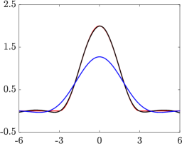
Figure 1: Example 5.1 - Exact solution $x^{\dagger}_{n}$ (red) and approximate solutions $x^{\delta,\ell}_{\alpha,n,i}$ computed by iAT (black) with $i=200$ and $\alpha$ determined by solving (18) and $x^{\delta,\ell}_{\alpha,n}$ computed by AT (blue) with $\alpha$ determined as in [34], for $n=1000$, $\ell=10$ and $\xi=0.01$, i.e. $\delta=1\%$.

Example 5.1.

Consider the Fredholm integral equation of the first kind discussed by Phillips [32]:

$$\int_{-6}^{6}\kappa(s,t)x(t)dt=y(s),\qquad-6\leq s\leq 6,$$

where the solution $x(t)$, the kernel $\kappa(s,t)$, and the right-hand side $y(s)$ are given by

$$x(t) =\begin{cases}1+\cos(\frac{\pi t}{3})&\text{if}\quad|t|<3,\\ 0&\text{if}\quad|t|\geq 3,\end{cases}$$

$$\kappa(s,t) =x(s-t),\qquad y(s)=(6-\arrowvert s\arrowvert)\left(1+\frac{1}{2}\cos\left(\frac{\pi s}{3}\right)\right)+\frac{9}{2\pi}\sin\left(\frac{\pi\arrowvert s\arrowvert}{3}\right).$$

We discretize this integral equation by a Nyström method based on the composite trapezoidal rule with $n$ nodes. This gives a nonsymmetric matrix $T_{n}\in\mathbb{R}^{n\times n}$ and the true solution $x_{n}^{\dagger}\in\mathbb{R}^{n}$. Table 1 shows the relative error $\|x_{n}^{\dagger}-x_{\alpha,n,i}^{\delta,\ell}\|_{2}/\|x_{n}^{\dagger}\|_{2}$ for several computed approximate solutions $x_{\alpha,n,i}^{\delta,\ell}$ for the noise level $\delta$ of $1\%$. The error depends on $y_{n}^{\delta}$, the matrix $T_{n}$, the approximation error (8), and the iteration number $i$. The relative error can be seen to decrease slowly as $\ell$ increases for fixed $i$, and to decrease quite rapidly as $i$ increases for fixed $\ell$. Moreover, $\alpha$ stabilizes when $i$ increases, independently of $\ell$. Figure 1 shows the exact solution as well as the approximate solutions computed with Algorithms 1 and 2. The latter algorithm can be seen to determine a much more accurate approximation of the exact solution $x_{n}^{\dagger}$ than the former.

The behavior of the relative error of approximate solutions computed with Algorithm 1 (AT) and Algorithm 2 (iAT) for varying $\alpha$ is displayed in Figure 2 in log-log scale. The $\alpha$-values determined by solving equation (14) are marked by “$*$” on the graphs. Note that the regularization parameters $\alpha$ obtained for the iAT method correspond to a point close to the minimum of the black curves, while the regularization parameters $\alpha$ for the AT method do not correspond to points on the red curves that are close to the minimum of these curves.

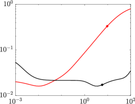
(a)

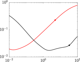
(b)

Figure 2: Example 5.1 - Relative error in approximate solutions computed by AT (red) and iAT (black) when varying $\alpha$ for $n=1000$ and $\xi=0.01$, i.e. $\delta=1\%$. The points marked by $\ast$ correspond to the value of $\alpha$ determined by solving (18) for iAT and as in [34] for AT. (a) $\ell=10$, $i=200$, (b) $\ell=30$, $i=100$.

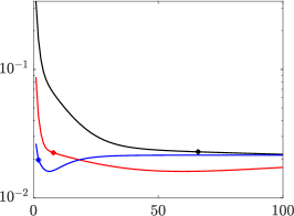
(a)

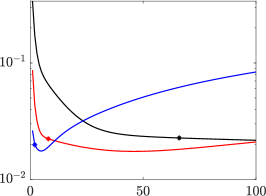
(b)

Figure 3: Example 5.1 - Relative error in approximate solutions computed by iAT as a function of $i$ for $\alpha=10$ (black), $\alpha=1$ (red), and $\alpha=0.1$ (blue), for $n=1000$ and $\xi=0.01$, i.e. $\delta=1\%$. The points marked by $*$ show when the discrepancy principle is satisfied; see Table 2. (a) $\ell=10$, (b) $\ell=30$.

We turn to the behaviour of Algorithm 2 for fixed values of $\alpha$ and determine the number of iterations $i$ by the discrepancy principle, i.e., we let $i$ be the smallest index such that

$$\|T_{n}x_{\alpha,n,i}^{\delta,\ell}-y_{n}^{\delta}\|_{2}\leq\delta.$$

Figure 3 shows the relative error in approximate solutions computed with Algorithm 2 as a function of $i$ for three values of $\alpha$ and $\ell=10$ (Figure 3 (a)) and $\ell=30$ (Figure 3 (b)). When $\alpha$ is small, it suffices to carry out a few iterations to satisfy the discrepancy principle at the cost of minor instability when increasing $i$. This behavior does not change much when increasing $\ell$. It is illustrated in Figure 3 (b) for $\ell=30$. The figure shows semi-convergence, i.e., that the error first decreases and subsequently increases when $i$ grows, to be more pronounced when $\alpha>0$ is small. Note that the discrepancy principle terminates the iterations for the same $i$-values for both $\ell$-values. Some relative errors in the computed approximate solutions are displayed in Table 2. We note that when $i=1$, the iterated Tikhonov method simplifies to a noniterated Tikhonov method. The latter differs from the AT method in [34] in that $\alpha$ is chosen differently. The relative errors in Table 2 are close to the smallest ones of Table 1, but are achieved with fewer $i$-iterations.

	$\ell=10$		$\ell=30$
$\alpha$	$i$	$\|x_{n}^{\dagger}-x_{\alpha,n,i}^{\delta,\ell}\|_{2}/\|x_{n}^{\dagger}\|_{2}$	$i$	$\|x_{n}^{\dagger}-x_{\alpha,n,i}^{\delta,\ell}\|_{2}/\|x_{n}^{\dagger}\|_{2}$
10	66	$2.28\cdot 10^{-2}$	66	$2.27\cdot 10^{-2}$
5	34	$2.27\cdot 10^{-2}$	34	$2.26\cdot 10^{-2}$
1	8	$2.24\cdot 10^{-2}$	8	$2.23\cdot 10^{-2}$
0.5	5	$2.18\cdot 10^{-2}$	5	$2.18\cdot 10^{-2}$
0.1	2	$1.97\cdot 10^{-2}$	2	$1.98\cdot 10^{-2}$
0.01	1	$1.61\cdot 10^{-2}$	1	$1.96\cdot 10^{-2}$

Table 2: Example 5.1 - Relative error in approximate solutions computed by iAT for fixed values of $\alpha$, and $i$ determined by the discrepancy principle for $n=1000$ and $\xi=0.01$, i.e. $\delta=1\%$.

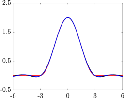
Figure 4: Example 5.1 - Exact solution $x_{n}^{\dagger}$ (red) and approximate solutions $x_{\alpha,n,i}^{\delta,\ell}$ (black) computed by iAT with $i=100$ and $\alpha$ determined by solving (18), and approximate solution $x_{0.1,n,2}^{\delta,\ell}$ (blue) computed by iAT using the discrepancy principle for $n=1000$, $\ell=30$, and $\xi=0.01$, i.e. $\delta=1\%$.

Figure 4 depicts the exact solution $x_{n}^{\dagger}$ as well as approximate solutions determined by Algorithm 2 for $\ell=30$. The approximate solution plotted in black is computed with Algorithm 2 (iAT) with $i=100$, and the approximate solution plotted in blue is determined by setting $\alpha=0.1$ and terminating the $i$-iterations with the discrepancy principle. Note that both computed approximate solutions are accurate approximations of $x_{n}^{\dagger}$.

Example 5.2.

We consider the Fredholm integral equation of the first kind discussed by Baart [3],

$$\int_{-6}^{6}\kappa(s,t)x(t)dt=y(s),\qquad 0\leq s\leq\frac{\pi}{2},$$

where

$$x(t)=\sin(t),\quad\kappa(s,t)=\exp(s\cos(t)),\quad\text{and}\quad y(s)=2\sinh(s)/s.$$

The discretization is determined with the MATLAB function baart from [22], which gives a nonsymmetric matrix $T_{n}\in\mathbb{R}^{n\times n}$ and the true solution $x_{n}^{\dagger}\in\mathbb{R}^{n}$.

	iAT			AT
$\ell$	$i$	$\alpha$	$\|x_{n}^{\dagger}-x_{\alpha,n,i}^{\delta,\ell}\|_{2}/\|x_{n}^{\dagger}\|_{2}$	$\|x_{n}^{\dagger}-x_{\alpha,n}^{\delta,\ell}\|_{2}/\|x_{n}^{\dagger}\|_{2}\ (\alpha)$
3	1	$1.23\cdot 10^{0\phantom{-}}$	$5.87\cdot 10^{-1}$	$7.48\cdot 10^{-1}\ (8.28)$
	200	$5.86\cdot 10^{0\phantom{-}}$	$3.67\cdot 10^{-1}$
	500	$2.03\cdot 10^{0\phantom{-}}$	$2.74\cdot 10^{-1}$
6	1	$1.27\cdot 10^{-1}$	$3.67\cdot 10^{-1}$	$4.25\cdot 10^{-1}\ (2.78\cdot 10^{-1})$
	200	$5.86\cdot 10^{0\phantom{-}}$	$3.04\cdot 10^{-1}$
	500	$2.03\cdot 10^{0\phantom{-}}$	$1.84\cdot 10^{-1}$
9	1	$5.44\cdot 10^{-2}$	$3.32\cdot 10^{-1}$	$3.37\cdot 10^{-1}\ (6.37\cdot 10^{-2})$
	200	$5.86\cdot 10^{0\phantom{-}}$	$3.05\cdot 10^{-1}$
	500	$2.03\cdot 10^{0\phantom{-}}$	$1.90\cdot 10^{-1}$

Table 3: Example 5.2 - Relative error in approximate solutions computed by iAT and $\alpha$ determined by solving $\eqref{alpha_iAT}$ for different values of $\ell$, with $n=1000$ and $\xi=0.01$, i.e. $\delta=1\%$. The AT method is applied with the parameter $\alpha$ determined as in [34].

	iAT			AT
$\ell$	$i$	$\alpha$	$\|x_{n}^{\dagger}-x_{\alpha,n,i}^{\delta,\ell}\|_{2}/\|x_{n}^{\dagger}\|_{2}$	$\|x_{n}^{\dagger}-x_{\alpha,n}^{\delta,\ell}\|_{2}/\|x_{n}^{\dagger}\|_{2}\ (\alpha)$
3	1	$6.51\cdot 10^{-1}$	$5.17\cdot 10^{-1}$	$7.14\cdot 10^{-1}\ (5.48)$
	500	$2.03\cdot 10^{0\phantom{-}}$	$1.28\cdot 10^{-1}$
	1000	$1.43\cdot 10^{0\phantom{-}}$	$4.60\cdot 10^{-2}$
6	1	$7.49\cdot 10^{-2}$	$3.42\cdot 10^{-1}$	$4.09\cdot 10^{-1}\ (2.32\cdot 10^{-1})$
	500	$2.03\cdot 10^{0\phantom{-}}$	$1.80\cdot 10^{-1}$
	1000	$1.43\cdot 10^{0\phantom{-}}$	$1.56\cdot 10^{-1}$
9	1	$2.29\cdot 10^{-3}$	$1.90\cdot 10^{-1}$	$2.15\cdot 10^{-1}\ (4.23\cdot 10^{-3})$
	500	$1.45\cdot 10^{0\phantom{-}}$	$1.74\cdot 10^{-1}$
	1000	$1.43\cdot 10^{0\phantom{-}}$	$1.65\cdot 10^{-1}$

Table 4: Example 5.2 - Relative error in approximate solutions computed by iAT and $\alpha$ determined by solving $\eqref{alpha_iAT}$ for different values of $\ell$, with $n=1000$ and $\xi=0.001$, i.e. $\delta=0.1\%$. The AT method is applied with the parameter $\alpha$ determined as in [34].

Table 3 shows the relative error in approximate solutions computed by the AT and iAT methods for $n=1000$ and noise level $\delta=1\%$. The singular values of the matrix $T_{n}$, when ordered in nonincreasing order, decreases very rapidly with increasing index. Therefore, it is not meaningful to choose $\ell$ larger than $9$. Algorithm 2 (iAT) can be seen to yield approximate solutions with smaller relative error than Algorithm 1 (AT), in particular for small values of $\ell$. Table 4 differs from Table 3 only in that the noise level is $\delta=0.1\%$.

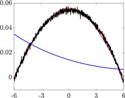
(a)

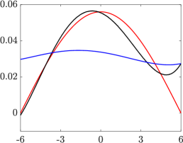
(b)

Figure 5: Example 5.2 - Exact solution $x^{\dagger}_{n}$ (red) and approximate solutions $x^{\delta,\ell}_{\alpha,n,i}$ computed by iAT (black) with $i=1000$ and $\alpha$ determined by solving (18) and $x^{\delta,\ell}_{\alpha,n}$ computed by AT (blue) with $\alpha$ determined as in [34], for $n=1000$, $\xi=0.001$, i.e. $\delta=0.1\%$. (a) $\ell=3$, (b) $\ell=6$.

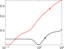
(a)

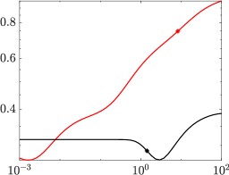
(b)

Figure 6: Example 5.2 - Relative error in approximate solutions computed by AT (red) and iAT (black) when varying $\alpha$ for $n=1000$, $\ell=3$ and $\xi=0.01$, i.e. $\delta=1\%$. The points marked by $\ast$ correspond to the value of $\alpha$ determined by solving (18) for iAT and as in [34] for AT. (a) $i=300$, (b) $i=1000$.

Figure 5 depicts the exact solution and computed approximate solutions for two values of $\ell$ and noise level $0.1\%$. These plots illustrate the improved quality of the computed solutions determined by the iAT method when compared with approximate solutions determined by the AT method. Figure 6 displays the behavior of the relative error in the computed approximate solutions when varying the parameter $\alpha$. The value of $\alpha$ for the iAT method, which is determined by solving (18), corresponds to a point that is closer to the minimum of the relative error than the point associated with the parameter value for the AT with $\alpha$ determined as in [34].

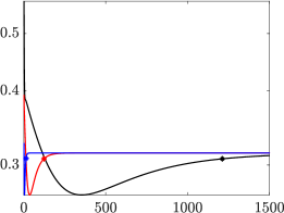
(a)

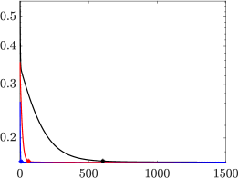
(b)

Figure 7: Example 5.2 - Relative error in approximate solutions computed by iAT as a function of $i$ for $\alpha=1$ (black), $\alpha=0.1$ (red), and $\alpha=0.01$ (blue), for $n=1000$ and $\xi=0.01$, i.e. $\delta=1\%$. The points marked by $*$ show when the discrepancy principle is satisfied; see Table 5. (a) $\ell=3$, (b) $\ell=9$.

We turn to the relative error of computed approximate solutions as a function of the iteration number $i$ for fixed values of $\alpha$. Figure 7 shows the relative error for three values of $\alpha$ and varying $i$ for two values of $\ell$. Note that, as expected, a larger $\ell$ gives a smaller error. Points marked by $*$ on the curves show the smallest $i$-values for which the discrepancy principle is satisfied. We note that the discrepancy principle is satisfied for a small $i$-value when $\alpha$ is small.

	$\ell=3$		$\ell=9$
$\alpha$	$i$	$\|x_{n}^{\dagger}-x_{\alpha,n,i}^{\delta,\ell}\|_{2}/\|x_{n}^{\dagger}\|_{2}$	$i$	$\|x_{n}^{\dagger}-x_{\alpha,n,i}^{\delta,\ell}\|_{2}/\|x_{n}^{\dagger}\|_{2}$
1	1212	$3.07\cdot 10^{-1}$	604	$1.68\cdot 10^{-1}$
0.1	123	$3.07\cdot 10^{-1}$	62	$1.68\cdot 10^{-1}$
0.01	14	$3.08\cdot 10^{-1}$	8	$1.67\cdot 10^{-1}$

Table 5: Example 5.2 - Relative error in approximate solutions computed by iAT for fixed values of $\alpha$, and $i$ determined by the discrepancy principle for $n=1000$ and $\xi=0.01$, i.e. $\delta=1\%$.

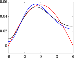
Figure 8: Example 5.2 - Exact solution $x_{n}^{\dagger}$ (red) and approximate solutions $x_{\alpha,n,i}^{\delta,\ell}$ (black) computed by iAT with $i=500$ and $\alpha$ determined by solving (18), and approximate solution $x_{0.1,n,62}^{\delta,\ell}$ (blue) computed by iAT using the discrepancy principle for $n=1000$, $\ell=9$, and $\xi=0.01$, i.e. $\delta=1\%$.

Table 5 displays the relative error when $i$ is determined by the discrepancy principle for three values of $\alpha$. The relative error in the computed approximate solution is essentially independent of the value of $\alpha$. For $\ell=9$ the results are comparable to those of Table 4. Figure 8 displays the exact solution for $n=1000$ (red curve) and computed solutions for $\ell=9$. The black curve displays the computed solution for $i=500$ for $\alpha$ determined by solving (18); the blue curve depicts the computed solution obtained by fixing $\alpha=0.1$ and determining $i$ with the discrepancy principle.

Example 5.3.

This example is concerned with a digital image deblurring problem. We use the function blur from [22] with default parameters to determine an $n^{2}\times n^{2}$ symmetric block Toeplitz matrix with Toeplitz blocks, $T_{n^{2}}$, that models blurring of an image that is represented by $n\times n$ pixels. The blur is determined by a space-invariant Gaussian point spread function. The true image is represented by the vector $x_{n^{2}}^{\dagger}\in\mathbb{R}^{n^{2}}$ for $n=30$. This image is shown in Figure 9 (a).

$i$	$\alpha$	$\|x_{n^{2}}^{\dagger}-x_{\alpha,n^{2},i}^{\delta,\ell}\|_{2}/\|x_{n^{2}}^{\dagger}\|_{2}$
1	$2.44\cdot 10^{1}$	$9.72\cdot 10^{-1}$
100	$3.36\cdot 10^{1}$	$3.68\cdot 10^{-1}$
200	$5.82\cdot 10^{0}$	$1.37\cdot 10^{-1}$
300	$3.24\cdot 10^{0}$	$9.01\cdot 10^{-2}$
400	$2.42\cdot 10^{0}$	$7.56\cdot 10^{-2}$
500	$2.02\cdot 10^{0}$	$6.83\cdot 10^{-2}$
1000	$1.42\cdot 10^{0}$	$6.05\cdot 10^{-2}$

Table 6: Example 5.3 - Relative error in approximate solutions computed by iAT and $\alpha$ determined by solving $\eqref{alpha_iAT}$ for $\ell=300$, $n^{2}=900$ and $\xi=0.01$, i.e. $\delta=1\%$.

Table 6 displays relative restoration errors for the computed approximate solutions with Algorithm 2 (iAT) for the noise level $\delta=1\%$. To satisfy inequality (15), we need to let $\ell>268$; any larger value of $\ell$ gives very similar results, in particular for a large number of iterations $i$. Therefore, we set $\ell=300$.

Figure 9 (b) shows the approximate solution computed with iAT for $\ell=300$ and $i=500$; $\alpha$ is determined by solving equation (18). For the AT method, we need at least $\ell=756$ to satisfy (15) with the choices $C=1$ and $E=3\|x_{n^{2}}^{\dagger}\|_{2}$. Figure 9 (c) shows the approximate solution computed by AT for $\ell=800$ and for $\alpha$ determined as in [34].

(a)

(b)

(c)

Figure 9: Example 5.3 - Exact solution $x^{\dagger}_{n}$ (a) and approximate solutions $x^{\delta,\ell}_{\alpha,n,i}$ computed by iAT (b) with $\ell=300$, $i=500$ and $\alpha$ determined by solving (18) and $x^{\delta,\ell}_{\alpha,n}$ computed by AT (c) with $\ell=800$ and $\alpha$ determined as in [34], for $n^{2}=900$, $\xi=0.01$, i.e. $\delta=1\%$.

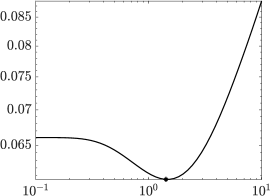
(a)

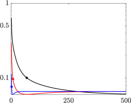
(b)

Figure 10: Example 5.2 - Relative error in approximate solutions computed by iAT for $n^{2}=900$, $\ell=300$ and $\xi=0.01$, i.e. $\delta=1\%$. (a) Relative error varying $\alpha$, where the point marked by $\ast$ correspond to the value of $\alpha$ determined by solving (18) with $i=1000$, (b) Relative error as a function of $i$ for $\alpha=1$ (black), $\alpha=0.1$ (red), and $\alpha=0.01$ (blue). The points marked by $*$ show when the discrepancy principle is satisfied; see Table 7.

$\alpha$	$i$	$\|x_{n^{2}}^{\dagger}-x_{\alpha,n^{2},i}^{\delta,\ell}\|_{2}/\|x_{n^{2}}^{\dagger}\|_{2}$
5	333	$1.01\cdot 10^{-1}$
1	68	$1.01\cdot 10^{-1}$
0.5	35	$9.99\cdot 10^{-2}$
0.1	8	$9.69\cdot 10^{-2}$
0.05	5	$9.08\cdot 10^{-2}$
0.01	2	$7.64\cdot 10^{-2}$
0.001	2	$6.43\cdot 10^{-2}$

Table 7: Example 5.3 - Relative error in approximate solutions computed by iAT for fixed values of $\alpha$, and $i$ determined by the discrepancy principle for $n^{2}=900$ and $\xi=0.01$, i.e. $\delta=1\%$.

Figure 10 displays the relative error of the computed solutions when varying the parameters $\alpha$ and $i$. Specifically, Figure 10(a) is obtained by varying $\alpha$ for $i=500$. The $*$ on the graph corresponds to the value of the parameter $\alpha$ determined by solving equation (18). Similarly, Figure 10 (b) is obtained by varying $i$ for three fixed values of $\alpha$. The $*$s mark $i$-values for which the discrepancy principle is satisfied. The robustness of the discrepancy principle is illustrated by Table 7, where for each $\alpha$, the number of iterations $i$ is determined by the discrepancy principle. The table displays the relative error in the computed approximate solutions.

We remark that the system matrix $T_{n^{2}}$ in this example is symmetric. Therefore, the symmetric Lanczos algorithm could be applied instead of the Arnoldi algorithm. However, computed examples reported in [2] show the latter algorithm to yield higher accuracy because the computed Lanczos vectors generated by the Lanczos algorithm may be far from orthogonal due to propagated and amplified round-off errors.

6 Conclusion and extensions

The paper presents a convergence analysis for iterated Tikhonov regularization based on the Arnoldi decomposition. A new approach to choosing the regularization parameter is proposed. Computed results show iterated Tikhonov regularization with the proposed parameter choice to yield more accurate approximate solutions than the non-iterative method studied in [34]. It would be interesting to extend this work to Tikhonov regularization in general form. Applications of such problems are described in e.g., [5, 6, 8, 9, 18, 23, 7]. It also may be interesting to compare the choice of regularization parameter of this paper with other parameter choices, such as those discussed in [24, 25, 26, 36].

Appendix A Appendix

This appendix discusses the technical details of the theory presented. Our analysis is carried out in infinite-dimensional spaces. We mainly extend techniques and findings from [31, 27] to the case of iterated Tikhonov. To the best of our knowledge, this is the first exploration of such an extension. Since this generalization poses nontrivial challenges and holds potential benefits for the analysis of other Tikhonov-type iterative methods, we believe that it deserves a dedicated section of its own. We use the same notation as in [31]. To enhance readability, we provide Table 8, which connects the notation of this appendix with the notation of Section 4.

Notation in Appendix A	$T$	$T_{h}$	$Q_{m}$	$T_{h,m}\coloneqq Q_{m}T_{h}$	$x^{\dagger}$	$x_{\alpha,m,i}^{\delta,h}$
Notation in Sections 3 and 4	$T_{n}$	$T_{n}^{(\ell)}$	$\mathcal{R}_{\ell}$	$T_{n}^{(\ell)}$	$x_{n}^{\dagger}$	$x_{\alpha,n,i}^{\delta,\ell}$

Table 8: Comparison of notations

A.1 Error estimates

Denote by $\mathcal{L}(\mathcal{X},\mathcal{Y})$ the space of linear operators from $\mathcal{X}$ to $\mathcal{Y}$. Let $T\in\mathcal{L}({\mathcal{X}},\mathcal{\mathcal{Y}})$ be a bounded linear operator and let $T_{h}$ be an approximation of $T$. We define, using the iterated Tikhonov (iT) method, the computed approximate solution

$$x_{\alpha,i}\coloneqq\sum\limits_{k=1}^{i}\alpha^{k-1}(T^{\ast}T+\alpha I)^{-k}T^{\ast}y$$ (iT)

of (1). When using $T_{h}$ instead of $T$, we obtain similarly $x_{\alpha,i}^{h}$.

Lemma A.1.

Let $x_{\alpha,i}$ be defined as in (iT). Then

$$\|x_{\alpha,i}-x_{\alpha,i}^{h}\|\leq i(i+1)\frac{\|T-T_{h}\|}{2\sqrt{\alpha}}\|x^{\dagger}\|+i\frac{\|Q_{h}(I-Q)y\|}{2\sqrt{\alpha}},$$ (19)

where $Q$ and $Q_{h}$ are the orthogonal projectors on $\overline{\operatorname{Rg}(T)}$ and $\overline{\operatorname{Rg}(T_{h})}$, respectively.

Proof.

We have

$$x_{\alpha,i}-x_{\alpha,i}^{h}=\sum\limits_{k=1}^{i}\alpha^{k-1}((T^{\ast}T+\alpha I)^{-k}-(T_{h}^{\ast}T_{h}+\alpha I)^{-k})T^{\ast}y+\sum\limits_{k=1}^{i}\alpha^{k-1}(T_{h}^{\ast}T_{h}+\alpha I)^{-k}(T^{\ast}-T_{h}^{\ast})y.$$ (20)

Using the simple algebraic identities for $A,B\in\mathcal{L}(\mathcal{X},\mathcal{Y})$,

$$A^{-k}-B^{-k}=B^{-k}(B^{k}-A^{k})A^{-k},\hskip 28.45274ptB^{k}-A^{k}=\sum\limits_{j=0}^{k-1}B^{j}(B-A)A^{k-1-j},$$

the first term in the right-hand side of (20) can be written as

$$\sum_{k=1}^{i}\sum\limits_{j=0}^{k-1}\alpha^{k-1}(T_{h}^{\ast}T_{h}+\alpha I)^{j-k}(T_{h}^{\ast}T_{h}-T^{\ast}T)(T^{\ast}T+\alpha I)^{-1-j}T^{\ast}Qy,$$

and using the fact that $T_{h}^{\ast}T_{h}-T^{\ast}T=T_{h}^{\ast}(T_{h}-T)+(T_{h}^{\ast}-T^{\ast})T$, we can split the above sum into

$$\sum_{k=1}^{i}\sum\limits_{j=0}^{k-1}\alpha^{k-1}(T_{h}^{\ast}T_{h}+\alpha I)^{j-k}T_{h}^{\ast}(T_{h}-T)(T^{\ast}T+\alpha I)^{-1-j}T^{\ast}Qy$$ (21a)

$$+\sum_{k=1}^{i}\sum\limits_{j=0}^{k-1}\alpha^{k-1}(T_{h}^{\ast}T_{h}+\alpha I)^{j-k}(T_{h}^{\ast}-T^{\ast})T(T^{\ast}T+\alpha I)^{-1-j}T^{\ast}Qy.$$ (21b)

Collecting factors $\alpha^{k-1}(T_{h}^{\ast}T_{h}+\alpha I)^{-k}$ from (21b) and the second term of (20), and using that $Qy=Tx^{\dagger}$ and $T^{\ast}_{h}=T^{\ast}_{h}Q_{h}$, their sum can be written as

$$\sum_{k=1}^{i}\alpha^{k-1}(T_{h}^{\ast}T_{h}+\alpha I)^{-k}\biggl{(}\sum_{j=0}^{k-1}(T_{h}^{\ast}T_{h}+\alpha I)^{j}(T_{h}^{\ast}-T^{\ast})T(T^{\ast}T+\alpha I)^{-1-j}T^{\ast}-(T_{h}^{\ast}-T^{\ast})\biggr{)}Tx^{\dagger}$$ (22a)

$$+\sum_{k=1}^{i}\alpha^{k-1}(T_{h}^{\ast}T_{h}+\alpha I)^{-k}T_{h}^{\ast}Q_{h}(Q-I)y.$$ (22b)

Now rewrite the term (22a) as

$$\sum_{k=1}^{i}\alpha^{k-1}(T_{h}^{\ast}T_{h}+\alpha I)^{-k}\biggl{(}-\alpha(T_{h}^{\ast}-T^{\ast})(TT^{\ast}+\alpha I)^{-1}\biggr{)}Tx^{\dagger}$$ (23a)

$$+\sum\limits_{k=1}^{i}\alpha^{k-1}(T_{h}^{\ast}T_{h}+\alpha I)^{-k}\biggl{(}\sum\limits_{j=1}^{k-1}(T_{h}^{\ast}T_{h}+\alpha I)^{j}(T_{h}^{\ast}-T^{\ast})T(T^{\ast}T+\alpha I)^{-1-j}T^{\ast}\biggr{)}Tx^{\dagger}.$$ (23b)

Thus, we obtain

$$\|x_{\alpha,i}-x_{\alpha,i}^{h}\|\leq\|\eqref{term1}\|+\|\eqref{term2}\|+\|\eqref{term3}\|+\|\eqref{term4}\|.$$

Collecting $\|T-T_{h}\|\|x^{\dagger}\|$ from the first three terms and $\|Q_{h}(Q-I)y\|$ from the last term, and using the bounds $\|(A^{\ast}A+\alpha I)^{-1}A^{\ast}A\|\leq 1$, $\|(A^{\ast}A+\alpha I)^{-1}A^{\ast}\|\leq 1/2\sqrt{\alpha}$ and similar by switching the position of $\ast$, inequality (19) follows.

For example, consider the argument of the nested sum (21a): Since $k-j-1\geq 0$ and $j\geq 0$, its norm is bounded as

$$\alpha^{k-1}\|(T_{h}^{\ast}T_{h}+\alpha I)^{j-k}T_{h}^{\ast}(T_{h}-T)(T^{\ast}T+\alpha I)^{-1-j}T^{\ast}Qy\|$$

$$\leq\alpha^{k-1}\|(T_{h}^{\ast}T_{h}+\alpha I)^{j-k+1}\|\|(T_{h}^{\ast}T_{h}+\alpha I)^{-1}T_{h}^{\ast}\|\|T-T_{h}\|\|(T^{\ast}T+\alpha I)^{-j}\|\|(T^{\ast}T+\alpha I)^{-1}T^{\ast}T\|\|x^{\dagger}\|$$

$$\leq\alpha^{k-1}\alpha^{j-k+1}(1/2\sqrt{\alpha})\|T-T_{h}\|\alpha^{-j}\|x^{\dagger}\|=\|T-T_{h}\|\|x^{\dagger}\|/2\sqrt{\alpha}.$$

Adding up all the terms, it follows that

$$\|\eqref{term1}\|+\|\eqref{term2}\|+\|\eqref{term3}\|\leq\frac{\|T-T_{h}\|}{2\sqrt{\alpha}}\|x^{\dagger}\|2\sum_{k=1}^{i}k=i(i+1)\frac{\|T-T_{h}\|}{2\sqrt{\alpha}}\|x^{\dagger}\|.$$

∎

Consider a family $\{W_{m}\}_{m\in\mathbb{N}}$ of finite-dimensional subspaces of $\mathcal{Y}$ such that the orthogonal projector $Q_{m}$ into $W_{m}$ converges to $I$ on $\overline{\operatorname{Rg}(T)}$. We define $x_{\alpha,m,i}^{h}$ and $x_{\alpha,m,i}^{\delta,h}$ similarly as in (iT), i.e., by replacing $T_{h}$ by $T_{h,m}\coloneqq Q_{m}T_{h}$ and using $y$ and $y^{\delta}$ as inputs, respectively. We now recall the useful [31, Assumptions 2.3]:

Assumption A.2.

Let $W_{m}\subset\mathcal{Y}$, $T_{h}\in\mathcal{L}(\mathcal{X},\mathcal{Y})$, $\delta\geq 0$, and $y^{\delta}\in\mathcal{Y}$ be such that

$$W_{m}\subset\overline{\operatorname{Rg}(T)},\hskip 85.35826pt \operatorname{Rg}(Q_{m}T_{h})=W_{m},$$

$$\|Q_{m}(T-T_{h})\|\leq h, \|Q_{m}(y-y^{\delta})\|\leq\delta.$$

The next two lemmas are preparatory to the proof of Proposition A.5.

Lemma A.3.

Under Assumptions A.2, we have

$$\|x^{\dagger}-x_{\alpha,m,i}^{\delta,h}\|\leq\alpha^{i}\|(T^{\ast}_{m}T_{m}+\alpha I)^{-i}x^{\dagger}\|+(i(i+1)h\|x^{\dagger}\|+i\delta)/2\sqrt{\alpha},$$

where $T_{m}\coloneqq Q_{m}T$.

Proof.

Let $x_{\alpha,m,i}$ be defined as in (iT) using $T_{m}\coloneqq Q_{m}T$. Then

$$\|x^{\dagger}-x_{\alpha,m,i}^{\delta,h}\|\leq\|x^{\dagger}-x_{\alpha,m,i}\|+\|x_{\alpha,m,i}-x_{\alpha,m,i}^{h}\|+\|x_{\alpha,m,i}^{h}-x_{\alpha,m,i}^{\delta,h}\|.$$

For the last term, we have the upper bound

$$\|x_{\alpha,m,i}^{h}-x_{\alpha,m,i}^{\delta,h}\|\leq\sum_{k=1}^{i}\|(T_{h,m}^{\ast}T_{h,m}+\alpha I)^{-1}T_{h,m}^{\ast}\|\|y-y^{\delta}\|\leq i\delta/2\sqrt{\alpha}.$$

For the first term, using $T_{m}x^{\dagger}=Q_{m}y$, we have

$$\|x^{\dagger}-x_{\alpha,m,i}\| =\Bigl{\|}x^{\dagger}-\sum_{k=1}^{i}\alpha^{k-1}(T_{m}^{\ast}T_{m}+\alpha I)^{-k}T_{m}^{\ast}T_{m}x^{\dagger}\Bigr{\|}$$

$$=\Bigl{\|}\alpha(T_{m}^{\ast}T_{m}+\alpha I)^{-1}x^{\dagger}-\sum_{k=2}^{i}\alpha^{k-1}(T_{m}^{\ast}T_{m}+\alpha I)^{-k}T_{m}^{\ast}T_{m}x^{\dagger}\Bigr{\|}$$

$$=\ldots$$

$$=\alpha^{i}\|(T_{m}^{\ast}T_{m}+\alpha I)^{-i}x^{\dagger}\|.$$ (24)

The upper bound for the second term is derived using Lemma A.1 by replacing $T$ by $T_{m}$, and $T_{h}$ by $T_{h,m}$. In accordance with Assumptions A.2, this yields

$$\|x_{\alpha,m,i}-x_{\alpha,m,i}^{h}\|\leq i(i+1)\frac{h}{2\sqrt{\alpha}}\|x^{\dagger}\|.$$

Combining the three bounds we have computed thus far, the thesis follows. ∎

For $\nu\geq 0$ and $\rho>0$, we introduce the set

$$\mathcal{X}_{\nu,\rho}\coloneqq\{x\in\mathcal{X}\mid x=(T^{\ast}T)^{\nu}w,\;w\in\ker(T)^{\perp}\mbox{ and }\|w\|\leq\rho\}.$$

Assuming that $x^{\dagger}\in\mathcal{X}_{\nu,\rho}$, we can bound (A.1) by

$$\|x^{\dagger}-x_{\alpha,m,i}\|\leq\alpha^{i}\|(T_{m}^{\ast}T_{m}+\alpha I)^{-i}(T_{m}^{\ast}T_{m})^{\nu}w\|+\|[(T^{\ast}T)^{\nu}-(T_{m}^{\ast}T_{m})^{\nu}]w\|.$$

Define

$$\gamma_{m}\coloneqq\|(I-Q_{m})T\|.$$

Lemma A.4.

Let $x^{\dagger}\in\mathcal{X}_{\nu,\rho}$ and let $w$ be fixed. Defining

$$b(\alpha,m)\coloneqq\alpha^{i(1-\nu)}\|(T_{m}^{\ast}T_{m}+\alpha I)^{-i}(T_{m}^{\ast}T_{m})^{\nu}w\|,$$

it holds that

$$\lim_{\begin{subarray}{c}m\rightarrow\infty\\ \alpha\rightarrow 0^{+}\end{subarray}}b(\alpha,m)=0$$

if $\nu\in[0,1)$ and

$$\gamma_{m}=o\Bigl{(}\mu_{m}^{\frac{\nu(i-1)}{1-\nu}}\Bigr{)},$$ (25)

for $\mu_{m}\coloneqq\min(\sigma(T^{\ast}_{m}T_{m})\setminus\{0\})$, where $\sigma(T_{m}^{\ast}T_{m})$ denotes the spectrum of $T_{m}^{\ast}T_{m}$.

Proof.

Letting $\{E_{\mu}^{m}\}_{\mu\in\mathbb{R}}$ be a spectral family for $T^{\ast}_{m}T_{m}$ (see e.g. [16, Section 2.3]) and $f_{\nu}(\mu)=\alpha^{i}(\mu+\alpha)^{-i}\mu^{\nu}$, we have the equality

$$b^{2}(\alpha,m)=\int_{0}^{\infty}\alpha^{-2i\nu}f_{\nu}^{2}(\mu)dE_{\mu}^{m}\|w\|^{2}.$$

By Hölder’s inequality,

$$b^{2}(\alpha,m) \leq\left[\int_{0}^{\infty}\left(\frac{\alpha}{\mu+\alpha}\right)^{2i}dE_{\mu}^{m}\|w\|^{2}\right]^{1-\nu}\left[\int_{0}^{\infty}\left(\frac{\mu}{(\mu+\alpha)^{i}}\right)^{2}dE_{\mu}^{m}\|w\|^{2}\right]^{\nu}$$

$$\leq\left[\int_{0}^{\infty}\left(\frac{\alpha}{\mu+\alpha}\right)^{2i}dE_{\mu}^{m}\|w\|^{2}\right]^{1-\nu}\mu_{m}^{2\nu(1-i)}\|w\|^{2\nu}.$$

Now

$$b^{\frac{1}{1-\nu}}(\alpha,m)\leq\mu_{m}^{\frac{\nu(1-i)}{1-\nu}}\alpha\|(T_{m}^{\ast}T_{m}+\alpha I)^{-1}w\|\|w\|^{\frac{\nu}{1-\nu}}\stackrel{{\scriptstyle\begin{subarray}{c}\alpha\to 0\\ m\to\infty\end{subarray}}}{{\longrightarrow}}0$$

follows from the proof of [27, Lemma 2.4]. ∎

Proposition A.5.

Let Assumptions A.2 and (25) be satisfied. Moreover, let $x^{\dagger}\in\mathcal{X}_{\nu,\rho}$. For $m$ sufficiently large, there is a unique $\alpha>0$ that solves

$$\alpha^{\frac{2i+1}{2}}\|(T_{m}^{\ast}T_{m}+\alpha I)^{-i}(T_{m}^{\ast}T_{m})^{\nu}w\|=(i(i+1)h\|x^{\dagger}\|+i\delta)/2.$$

Moreover, it holds $\alpha\rightarrow 0$ for $m\rightarrow\infty$, $h,\delta\rightarrow 0$, and if $\sqrt{\alpha}=o\Bigl{(}\mu_{m}^{\frac{\nu(i-1)}{1-\nu}}\Bigr{)}$, then we have

$$\|x^{\dagger}-x_{\alpha,m,i}^{\delta,h}\|=\begin{cases}o(1)&\text{if $\nu=0$,}\\ o((h+\delta)^{\frac{2i\nu}{2i\nu+1}})+O(\gamma_{m}^{2\nu}\|w\|)&\text{if $0<\nu<1$,}\\ O((h+\delta)^{\frac{2i}{2i+1}})+O(\gamma_{m}\|(I-Q_{m})Tw\|)&\text{if $\nu=1$.}\end{cases}$$

Proof.

Follows from Lemma A.3 and Lemma A.4 analogously to [31, Proposition 2.6] and [27, Theorem 2.1]. ∎

A.2 The parameter choice method

We describe an a posteriori parameter choice method for Algorithm 2 in Section 4. Define

$$f(m,\alpha,w,A)\coloneqq\alpha^{2i+1}\langle(A_{m}A^{\ast}_{m}+\alpha I)^{-2i-1}Q_{m}w,Q_{m}w\rangle,$$

where $A_{m}\coloneqq Q_{m}A$ and $\langle\cdot,\cdot\rangle$ denotes the Euclidean scalar product.

Proposition A.6.

Let $C$ and $E$ be positive constants such that

$$Eh+C\delta\leq\|Q_{m}y^{\delta}\|.$$ (26)

Then there is a unique $\alpha>0$ that solves

$$f(m,\alpha,y^{\delta},T_{h})=(Eh+C\delta)^{2}.$$ (27)

Proof.

Analogous to [31, Proposition 3.1]. ∎

We now extend the result of [31, Lemma 3.2], which will be used in Theorem A.8.

Lemma A.7.

Let $A,B\in\mathcal{L}(\mathcal{X},\mathcal{Y})$. Then

$$\alpha^{\frac{2i+1}{2}}\|[(AA^{\ast}+\alpha I)^{-\frac{2i+1}{2}}-(BB^{\ast}+\alpha I)^{-\frac{2i+1}{2}}]A\|\leq(2i+1)\|A-B\|.$$

Proof.

We rewrite the element in the square brackets as

$$\sum\limits_{k=0}^{i-1}(BB^{\ast}+\alpha I)^{k-\frac{2i+1}{2}}(BB^{\ast}-AA^{\ast})(AA^{\ast}+\alpha I)^{-1-k}$$

$$+(BB^{\ast}+\alpha I)^{-\frac{1}{2}}((BB^{\ast}+\alpha I)^{\frac{1}{2}}-(AA^{\ast}+\alpha I)^{\frac{1}{2}})(AA^{\ast}+\alpha I)^{-\frac{2i+1}{2}}.$$

For the first term, we use $BB^{\ast}-AA^{\ast}=B(B^{\ast}-A^{\ast})+(B-A)A^{\ast}$, obtaining

$$\alpha^{\frac{2i+1}{2}}\Bigl{\|}\sum_{k=0}^{i-1}(BB^{\ast}+\alpha I)^{k-\frac{2i+1}{2}}(BB^{\ast}-AA^{\ast})(AA^{\ast}+\alpha I)^{-1-k}A\Bigr{\|}\leq 2i\|A-B\|.$$

The second term is bounded from above by

$$\alpha^{\frac{3}{2}}\|(BB^{\ast}+\alpha I)^{-\frac{1}{2}}((BB^{\ast}+\alpha I)^{\frac{1}{2}}-(AA^{\ast}+\alpha I)^{\frac{1}{2}})(AA^{\ast}+\alpha I)^{-\frac{3}{2}}A\|$$

and the thesis follows from the proof of [31, Lemma 3.2]. ∎

Theorem A.8.

Let $C>1$ and $E>(2i+1)\|x^{\dagger}\|$. For each $(W_{m},h,T_{h},\delta,y^{\delta})$, let Assumptions A.2, (25), and (26) be fulfilled. Moreover, let $x^{\dagger}\in\mathcal{X}_{\nu,\rho}$ and let $\alpha>0$ be the unique solution of (27). Then, if $\sqrt{\alpha}=o\Bigl{(}\mu_{m}^{\frac{\nu(i-1)}{1-\nu}}\Bigr{)}$, the same asymptotic estimates of Proposition A.5 hold for this parameter choice.

Proof.

The result follows from Lemma A.7 analogously to [31, Lemma 3.3, Proposition 3.4, Theorem 3.5]. ∎

We now extend the result of [31, Proposition 3.6].

Proposition A.9.

Let $C=1$ and $E=\|x^{\dagger}\|$. Let (26) be satisfied and let $\alpha>0$ be the unique solution of (27). Then, for all $\tilde{\alpha}\geq\alpha$, it holds that $\|x^{\dagger}-x_{\alpha,m,i}^{\delta,h}\|\leq\|x^{\dagger}-x_{\tilde{\alpha},i,m}^{\delta,h}\|$.

Proof.

Let $\{F_{\mu}^{h,m}\}_{\mu\in\mathbb{R}}$ be a spectral family for $T_{h,m}T^{\ast}_{h,m}$ and define $e(\alpha)\coloneqq\frac{1}{2}\|x^{\dagger}-x_{\alpha,m,i}^{\delta,h}\|^{2}$. Then

$$\frac{de(\alpha)}{d\alpha}=i\biggl{\langle}T_{h,m}x^{\dagger}-\int_{0}^{\infty}\frac{(\mu+\alpha)^{i}-\alpha^{i}}{(\mu+\alpha)^{i}}dF_{\mu}^{h,m}Q_{m}y^{\delta},\int_{0}^{\infty}\frac{\alpha^{i-1}}{(\mu+\alpha)^{i+1}}dF_{\mu}^{h,m}Q_{m}y^{\delta}\biggr{\rangle}.$$

Now, adding and subtracting $i\alpha^{2i-1}\bigl{\|}(T_{h,m}T_{h,m}^{\ast}+\alpha I)^{\frac{-2i-1}{2}}Q_{m}y^{\delta}\bigr{\|}^{2}$, we obtain

$$\frac{de(\alpha)}{d\alpha} =i\alpha^{2i-1}\bigl{\|}(T_{h,m}T_{h,m}^{\ast}+\alpha I)^{\frac{-2i-1}{2}}Q_{m}y^{\delta}\bigr{\|}^{2}$$

$$+i\biggl{\langle}\int_{0}^{\infty}\frac{\alpha^{i-1}}{(\mu+\alpha)^{\frac{1}{2}}}dF_{\mu}^{h,m}(T_{h,m}x^{\dagger}-Q_{m}y^{\delta}),(T_{h,m}T_{h,m}^{\ast}+\alpha I)^{\frac{-2i-1}{2}}Q_{m}y^{\delta}\biggr{\rangle}.$$

Thus, collecting $i\bigl{\|}(T_{h,m}T_{h,m}^{\ast}+\alpha I)^{\frac{-2i-1}{2}}Q_{m}y^{\delta}\bigr{\|}\eqqcolon K$ from the two terms above, we have

$$\frac{de(\alpha)}{d\alpha}\geq K\left(\alpha^{2i-1}\bigl{\|}(T_{h,m}T_{h,m}^{\ast}+\alpha I)^{\frac{-2i-1}{2}}Q_{m}y^{\delta}\bigr{\|}-\biggl{\|}\int_{0}^{\infty}\frac{\alpha^{i-1}}{(\mu+\alpha)^{\frac{1}{2}}}dF_{\mu}^{h,m}(T_{h,m}x^{\dagger}-Q_{m}y^{\delta})\biggr{\|}\right).$$

The thesis follows from

$$\biggl{\|}\int_{0}^{\infty}\frac{\alpha^{i-1}}{(\mu+\alpha)^{\frac{1}{2}}}dF_{\mu}^{h,m}(T_{h,m}x^{\dagger}-Q_{m}y^{\delta})\biggr{\|}\leq\alpha^{i-\frac{3}{2}}\|T_{h,m}x^{\dagger}-Q_{m}y^{\delta}\|$$

similarly as [31, Proposition 3.6]. ∎

Analogously to [31, Remark 3.7], if an estimation of $\|x^{\dagger}\|$ is not available, then the function $D\|x_{\alpha,m,i}^{\delta,h}\|$ with a constant $D\geq 1$ can be used in place of $\|x^{\dagger}\|$ to define the constant $E$. It can be shown that, for $\alpha$ satisfying (27) with this choice, we achieve the same rates of convergence as presented in Theorem A.8.

A.3 Other convergence rates

We derive results on the convergence rates similar to the ones of [41, 19, 39] for (iT), and provide a brief description of all cases $\nu\geq 0$. The main difference here is that we no longer require the hypothesis on $\mu_{m}$, i.e., on the spectrum of $T^{\ast}_{m}T_{m}$, to be satisfied, which leads to slower convergence rates.

Lemma A.10.

If $\nu\in[0,i)$, then it holds

$$\lim\limits_{\begin{subarray}{c}m\rightarrow\infty\\ \alpha\rightarrow 0^{+}\end{subarray}}\alpha^{i-\nu}\|(T_{m}^{\ast}T_{m}+\alpha I)^{-i}(T_{m}^{\ast}T_{m})^{\nu}w\|=0.$$

Proof.

Analogous to Lemma A.4. ∎

Proposition A.11.

Let Assumptions A.2 be satisfied and let $x^{\dagger}\in\mathcal{X}_{\nu,\rho}$. Let $\alpha>0$ be as in Proposition A.5. Then we have

$$\|x^{\dagger}-x_{\alpha,m,i}^{\delta,h}\|=\begin{cases}o(1)&\text{if $\nu=0$,}\\ o((h+\delta)^{\frac{2\nu}{2\nu+1}})+O(\gamma_{m}^{2\nu}\|w\|)&\text{if $0<\nu<i$,}\\ O((h+\delta)^{\frac{2i}{2i+1}})+O(\gamma_{m}\|(I-Q_{m})Tw\|)&\text{if $\nu=i$.}\end{cases}$$

Proof.

Follows from Lemma A.10 analogously to Proposition A.5. ∎

Results similar to those of Section A.2 on the parameter choice method, and of Proposition 4.2 and its corollaries, remain valid for $\nu\in[0,i]$. For the case $\nu>i$, we have the following result.

Proposition A.12.

Let Assumptions A.2 hold and let $x^{\dagger}\in\mathcal{X}_{\nu,\rho}$ with $\nu>i$. For $\alpha=(h+\delta)^{\frac{2}{2i+1}}$, we have

$$\|x^{\dagger}-x_{\alpha,m,i}^{\delta,h}\|=O((h+\delta)^{\frac{2i}{2i+1}})+\|[(T^{\ast}T)^{\nu}-(T_{m}^{\ast}T_{m})^{\nu}]w\|.$$

Proof.

Analogous to the first part of Proposition A.5. ∎

References

- [1] P. Alba, L. Fermo, C. Mee and G. Rodriguez “Recovering the electrical conductivity of the soil via a linear integral model” In Journal of Computational and Applied Mathematics 352 Elsevier, 2019, pp. 132–145
- [2] M. Alkilayh and L. Reichel “Some numerical aspects of Arnoldi-Tikhonov regularization” In Applied Numerical Mathematics 185 Elsevier, 2023, pp. 503–515
- [3] M. L. S. Baart “The use of auto-correlation for pseudo-rank determination in noisy ill-conditioned linear least-squares problems” In IMA Journal of Numerical Analysis 2 Oxford Univeristy Press, 1982, pp. 241–247
- [4] A. H. Bentbib, M. El Guide, K. Jbilou, E. Onunwor and L. Reichel “Solution methods for linear discrete ill-posed problems for color image restoration” In BIT Numerical Mathematics 58 Springer, 2018, pp. 555–578
- [5] D. Bianchi, A. Buccini, M. Donatelli and E. Randazzo “Graph Laplacian for image deblurring” In Electronic Transactions on Numerical Analysis 55 Kent State University, 2022, pp. 169–186
- [6] D. Bianchi, A. Buccini, M. Donatelli and S. Serra-Capizzano “Iterated fractional Tikhonov regularization” In Inverse Problems 31, 2015, pp. 055005
- [7] Davide Bianchi and Marco Donatelli “On generalized iterated Tikhonov regularization with operator-dependent seminorms” In Electronic Transactions on Numerical Analysis 47, 2017, pp. 73–99
- [8] Davide Bianchi, Marco Donatelli, Davide Evangelista, Wenbin Li and Elena Loli Piccolomini “Graph Laplacian and Neural Networks for Inverse Problems in Imaging: GraphLaNet” In International Conference on Scale Space and Variational Methods in Computer Vision, 2023, pp. 175–186
- [9] Davide Bianchi, Guanghao Lai and Wenbin Li “Uniformly convex neural networks and non-stationary iterated network Tikhonov (iNETT) method” In Inverse Problems 39.5, 2023, pp. 055002
- [10] C. Boor “A Practical Guide to Splines” Springer, 1978
- [11] Alessandro Buccini, Marco Donatelli and Lothar Reichel “Iterated Tikhonov regularization with a general penalty term” In Numerical Linear Algebra with Applications 24.4, 2017, pp. e2089
- [12] Alessandro Buccini, Lucas Onisk and Lothar Reichel “An Arnoldi-based preconditioner for iterated Tikhonov regularization” In Numerical Algorithms 92.1 Springer, 2023, pp. 223–245
- [13] D. Calvetti, S. Morigi, L. Reichel and F. Sgallari “Tikhonov regularization and the L-curve for large discrete ill-posed problems” In Journal of Computational and Applied Mathematics 123.1-2, 2000, pp. 423–446
- [14] Marco Donatelli “On nondecreasing sequences of regularization parameters for nonstationary iterated Tikhonov” In Numerical Algorithms 60 Springer, 2012, pp. 651–668
- [15] Marco Donatelli and Martin Hanke “Fast nonstationary preconditioned iterative methods for ill-posed problems, with application to image deblurring” In Inverse Problems 29.9 IOP Publishing, 2013, pp. 095008
- [16] H. W. Engl, M. Hanke and A. Neubauer “Regularization of Inverse Problems” Kluwer, Dordrecht, 1996
- [17] Silvia Gazzola and James G Nagy “Generalized Arnoldi-Tikhonov method for sparse reconstruction” In SIAM Journal on Scientific Computing 36.2, 2014, pp. B225–B247
- [18] Silvia Gazzola, Paolo Novati and Maria Rosaria Russo “On Krylov projection methods and Tikhonov regularization” In Electronic Transactions on Numerical Analysis 44, 2015, pp. 83–123
- [19] H. Gfrerer “An A Posteriori Parameter Choice for Ordinary and Iterated Tikhonov Regularization of Ill-Posed Problems Leading to Optimal Convergence Rates” In Mathematics of Computation 49, 1987, pp. 523–542
- [20] R. W. Goodman “Discrete Fourier and Wavelet Transforms: An Introduction Through Linear Algebra with Applications to Signal Processing” World Scientific Publishing Company, London, 2016
- [21] Martin Hanke and Charles W Groetsch “Nonstationary iterated Tikhonov regularization” In Journal of Optimization Theory and Applications 98 Springer, 1998, pp. 37–53
- [22] Per C. Hansen “Regularization tools version 4.0 for Matlab 7.3” In Numerical Algorithms 46, 2007, pp. 189–194
- [23] Guangxin Huang, Lothar Reichel and Feng Yin “On the choice of subspace for large-scale Tikhonov regularization problems in general form” In Numerical Algorithms 81, 2019, pp. 33–55
- [24] K Kanagaraj, GD Reddy and Santhosh George “Discrepancy principles for fractional Tikhonov regularization method leading to optimal convergence rates” In Journal of Applied Mathematics and Computing 63, 2020, pp. 87–105
- [25] S. Kindermann “Convergence analysis of minimization-based noise level-free parameter choice rules for linear ill-posed problems” In Electronic Transactions on Numerical Analysis 38, 2011, pp. 233–257
- [26] S. Kindermann and K. Raik “A simplified L-curve method as error estimator” In Electronic Transactions on Numerical Analysis 53, 2020, pp. 217–238
- [27] J. T. King and A. Neubauer “A variant of finite-dimensional Tikhonov regularization with a-posteriori parameter choice” In Computing 40, 1988, pp. 91–109
- [28] Bryan Lewis and Lothar Reichel “Arnoldi-Tikhonov regularization methods” In Journal of Computational and Applied Mathematics 226, 2009, pp. 92–102
- [29] F. Natterer “Regularization of ill-posed problems by projection methods” In Numererische Mathematik 28, 1977, pp. 329–341
- [30] F. Natterer “The Mathematics of Computerized Tomography” SIAM, Philadelphia, 2001
- [31] A. Neubauer “An a posteriori parameter choice for Tikhonov regularization in the presence of modeling error” In Applied Numerical Mathematics 4, 1988, pp. 507–519
- [32] D. L. Phillips “A technique for the numerical solution of certain integral equations of the first kind” In Journal of the ACM 9 ACM, 1962, pp. 84–97
- [33] S. Raffetseder, R. Ramlau and M. Yudytski “Optimal mirror deformation for multi-conjugate adaptive optics systems” In Inverse Problems 32, 2016, pp. 025009
- [34] R. Ramlau and L. Reichel “Error estimates for Arnoldi-Tikhonov regularization for ill-posed operator equations” In Inverse Problems 35, 2019, pp. 055002
- [35] R. Ramlau and M. Rosensteiner “An efficient solution to the atmospheric turbulence tomography problem using Kaczmarz iteration” In Inverse Problems 28 IOP publishing, 2012, pp. 095004
- [36] GD Reddy “A class of parameter choice rules for stationary iterated weighted Tikhonov regularization scheme” In Applied Mathematics and Computation 347, 2019, pp. 464–476
- [37] L. Reichel and Q. Ye “Breakdown-free GMRES for singular systems” In SIAM Journal on Matrix Analysis and Applications 26.4, 2005, pp. 1001–1021
- [38] Y. Saad “Iterative Methods for Sparse Linear Systems” SIAM, Philadelphia, 2003
- [39] O. Scherzer “Convergence rates of iterated Tikhonov regularized solutions of nonlinear Ill-posed problems” In Numerische Mathematik 66 Springer-Verlag, 1993, pp. 259–279
- [40] O. Scherzer, M. Grasmair, H. Grossauer, M. Haltmeier and F. Lenzen “Variational Methods in Imaging” Springer, New York, 2009
- [41] S. Yang, X. Xiong, P. Pan and Y. Sun “Stationary iterated weighted Tikhonov regularization method for identifying an unknown source term of time-fractional radial heat equation” In Numerical Algorithms 90, 2022, pp. 881–903