Cross-View Graph Consistency Learning for Invariant Graph Representations

Abstract

Graph representation learning is fundamental for analyzing graph-structured data. Exploring invariant graph representations remains a challenge for most existing graph representation learning methods. In this paper, we propose a cross-view graph consistency learning (CGCL) method that learns invariant graph representations for link prediction. First, two complementary augmented views are derived from an incomplete graph structure through a bidirectional graph structure augmentation scheme. This augmentation scheme mitigates the potential information loss that is commonly associated with various data augmentation techniques involving raw graph data, such as edge perturbation, node removal, and attribute masking. Second, we propose a CGCL model that can learn invariant graph representations. A cross-view training scheme is proposed to train the proposed CGCL model. This scheme attempts to maximize the consistency information between one augmented view and the graph structure reconstructed from the other augmented view. Furthermore, we offer a comprehensive theoretical CGCL analysis. This paper empirically and experimentally demonstrates the effectiveness of the proposed CGCL method, achieving competitive results on graph datasets in comparisons with several state-of-the-art algorithms.

I Introduction

Graph neural networks (GNNs), inheriting the representation learning advantages of traditional deep neural networks [26, 14, 1, 3, 19], have become increasingly popular for analyzing graph-structured data [8]. Graph representation learning (GRL) aims to learn meaningful node embeddings, referred to as graph representations, from both graph structures and node features via GNNs [11]. Graph representations have been extensively applied in downstream tasks, e.g., link prediction. Link prediction seeks to predict the missing connections between node pairs from an incomplete graph structure. It shows the significant impact of developing applications with graph-structured data [15], including citation network analysis [12], social network analysis [12] and recommendation systems [27].

In recent years, many research efforts have been directed toward investigating GNNs for GRL. For example, several classic GNN models have been proposed to learn meaningful graph representations from graph-structured data, such as graph convolutional network (GCN) [11], variational graph autoencoder (VGAE) [10], graph attention network [24], graph sampling and aggregation (GraphSAGE) [6] and their variants [21, 12]. These methods have achieved impressive link prediction results. However, the potential of utilizing graph structures for the available graph-structured data has not been fully exploited.

Self-supervised learning has recently emerged as a promising representation learning paradigm for GNNs [9, 23]. It can learn latent graph representations from unlabeled graph-structured data by supervision, which is provided by the data itself with different auxiliary learning tasks. Most self-supervised learning-based algorithms fall into two categories: contrastive learning [2, 13, 7, 28] and generative learning [21, 12, 9, 5]. For example, Hassani et al. [7] presented a contrastive multiview representation learning (CMRL) method that learns graph representations by contrasting encodings derived from first-order neighbors and a graph diffusion module. The feature pairs may have different data distributions under the two different types of augmented views. This may have a significant negative impact on measuring the similarity between positive pairs and the dissimilarity between negative pairs when conducting contrastive learning. Li et al. [12] presented a masked graph autoencoder (MGAE) method that reconstructs a complete graph structure by masking a portion of the observed edges. By randomly masking a portion of the edges, the MGAE method somewhat reduces the redundancy of the graph autoencoder (GAE) in self-supervised graph learning tasks. The randomness of edge masking causes a sampling information loss problem. Consequently, this is an increasing concern regarding the capture of the complementary information between the augmented views of a graph.

A vast majority of the available contrastive learning-based GRL methods consider their GNN-based models to be independent of different downstream tasks [21, 30]. Recent advances have shown that the optimal data augmentation views critically depend on the downstream tasks involving the visual data [25, 22]. The augmented views of the visual data share as little information as necessary to maximize the task-relevant mutual information. Motivated by this, we further investigate how to take full advantage of graph structure information and simultaneously retain the task-relevant information needed by a specific downstream task, i.e., link prediction. This is beneficial for learning invariant graph representations from the augmented views of graph-structured data, which is central to enhancing the ability of a model to produce general graph representations.

In this paper, we propose a cross-view graph consistency learning (CGCL) method that learns invariant graph representations for link prediction. Numerous missing connections are involved in the graph structure. We first construct two complementary augmented views of the graph structure of interest from the remainder of the link connections. Then, we propose a cross-view training scheme to train the proposed CGCL model, which can produce invariant graph representations for graph structure reconstruction purposes. The proposed cross-view training scheme attempts to maximize the consistency information between one augmented view and the graph structure reconstructed from the other augmented view. In contrast with randomly performing edge perturbation, node dropping or attribute masking, this approach can prevent the loss of valuable information contained in raw graph-structured data during GRL. Moreover, the complementary information in the graph structure can be further exploited by virtue of the cross-view training scheme. In addition, a comprehensive theoretical analysis is provided to reveal the supervisory information connections between the two complementary augmented views.

The key contributions are summarized as follows.

• We present a bidirectional graph structure augmentation scheme to construct two complementary augmented views of a graph structure.

• We propose a CGCL model that can learn invariant graph representations for link prediction.

• A cross-view training scheme is proposed to train the CGCL model by maximizing the consistency information between one augmented view and the graph structure reconstructed from the other augmented view.

• Extensive experiments are conducted on graph datasets, achieving competitive results.

II Related Work

An undirected graph $\mathcal{G}$ is defined as $\mathcal{G}=\left({\mathcal{V},\mathcal{E}}\right)$, where $\mathcal{V}=\left\{{{v_{1}},...,{v_{n}}}\right\}$ and $\mathcal{E}=\left\{{{e_{1}},...,{e_{m}}}\right\}$ stand for a set of $n$ nodes and a set of $m$ edges, respectively [11]. Each node $v_{i}$ in $\mathcal{V}$ is associated with a corresponding feature $x_{i}$ $\left({1\leq i\leq n}\right)\in{\mathbb{R}^{d}}$. An adjacency matrix of a graph structure $\mathbf{A}\in{\mathbb{R}^{n\times n}}$ is employed to represent the relationships among the nodes, where ${A_{ij}}=1$ indicates that an edge exists between nodes $v_{i}$ and $v_{j}$ and vice versa. The degree matrix $\mathbf{D}$ is defined as $\mathbf{D}=diag\left[{{d_{1}},{d_{2}},...,{d_{n}}}\right]\in{\mathbb{R}^{n\times n}}$, and its diagonal elements are ${d_{i}}=\sum\nolimits_{{v_{j}}\in V}{{A_{ij}}}$.

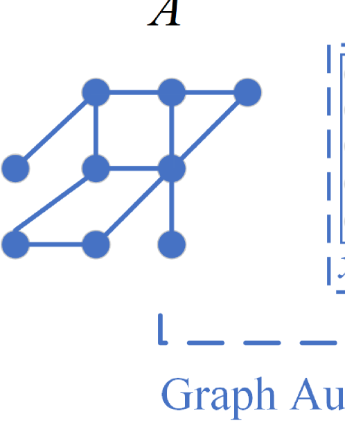
Figure 1: Framework of the CGCL model. Each augmented view of a graph structure, ${\mathbf{A}_{i}}$ $\left({i=1,2}\right)$, corresponds to three modules, including an augmented graph structure module, a shared GCN encoder module and a shared cross-view consistency decoder module. $\mathbf{A}$ and $\widetilde{\mathbf{A}}$ represent the incomplete graph structure and predictive graph structure, respectively.

II-A Self-Supervised GRL

A GCN learns node embeddings for graph-structured data [11]. Given an undirected graph $\mathcal{G}$, $\widetilde{\mathbf{A}}=\mathbf{A}+\mathbf{I}$ is the adjacency matrix of this undirected graph $\mathcal{G}$ with an added self-loop, and ${\widetilde{\mathbf{D}}}$ is a diagonal degree matrix ${\widetilde{D}_{ii}}=\sum\nolimits_{j}{{{\widetilde{A}}_{ij}}}$. The formula for the -th GCN layer is defined as

$$\begin{split}{\mathbf{H}^{(l)}}&={f^{(l)}}\left({\mathbf{A},{\mathbf{H}^{(l-1)}};{\mathbf{W}^{(l)}}}\right)\\ &=\sigma\left({{{\widetilde{\mathbf{D}}}^{-{1\mathord{\left/{\vphantom{12}}\right.\kern-1.2pt}2}}}{\widetilde{\mathbf{A}}}{{\widetilde{\mathbf{D}}}^{-{1\mathord{\left/{\vphantom{12}}\right.\kern-1.2pt}2}}}{\mathbf{H}^{(l-1)}}{\mathbf{W}^{(l)}}}\right)\\ \end{split}$$ (1)

where $l$ denotes the $l$th layer, ${\mathbf{W}^{(l)}}$ is a layer-specific learnable weight matrix, ${\mathbf{H}^{(l)}}$ is the node embedding matrix with $\mathbf{H}^{(0)}=\mathbf{X}$, and $\sigma$ is a nonlinear activation function, e.g., ${\rm ReLU}\left(\cdot\right)=\max\left({0,\cdot}\right)$. For a semi-supervised classification task, the weight parameters in the GCN model can be learned by minimizing the cross-entropy error between the ground truth and predictive the labels [11].

Contrastive learning-based GRL methods follow the principle of mutual information maximization by contrasting positive and negative pairs [28, 7, 30]. Data augmentation is a key prerequisite for these GRL methods. For example, You et al. [28] presented a graph-contrastive learning framework that provides four types of graph augmentation strategies, including node dropping, edge perturbation, attribute masking and subgraph production, to improve the generalizability of the graph representations produced during GNN pretraining.

Generative learning-based GRL methods aim to reconstruct graph data for learning graph representations [21, 12, 10]. For example, a VGAE employs two GCN models to build its encoder component, which can learn meaningful node embeddings for the reconstruction of a graph structure [10]. Lousi et al. [16] presented a scalable simplified subgraph representation learning method (S3GRL) that simplifies the message passing and aggregation operations in the subgraph of each link. Additionally, several GAE-based GRL methods employ different masking strategies on a graph structure to implement graph augmentation, including a masked GAE (GraphMAE) [9], an MGAE [12] and a self-supervised GAE (S2GAE) [21]. After randomly making a portion of the edges on a graph structure, these GRL methods attempt to reconstruct the missing connections with a partially visible, unmasked graph structure.

III Cross-View Graph Consistency Learning

In this section, we present the proposed CGCL method in detail, which produces invariant graph representations for self-supervised graph learning. These graph representations can be employed on a specific downstream task, i.e., the reconstruction of an incomplete graph structure.

III-A Problem Formulation

Let $\mathbf{X}\in{\mathbb{R}^{n\times d}}$ be a matrix consisting of features, each row of which corresponds to a node feature. Given an undirected graph $\mathcal{G}$ with an incomplete graph structure and the above features $\mathbf{X}$, the goal of our work is to learn graph representations, which can be employed to reconstruct the incomplete graph structure for link prediction.

III-B Network Architecture

The proposed CGCL method aims to produce the complete graph structure by predicting the missing connections. Fig. 1 provides an overview of the proposed CGCL network architecture, which is composed of three main modules, i.e., an augmented graph structure module, a shared GCN encoder module and a shared cross-view consistency decoder module. The augmented graph structure module is utilized to generate two complementary augmented views of the original graph structure. Inspired by the VGAE [10], the shared GCN encoder module learns individual graph structures for each augmented view under unsupervised representation learning. The cross-view consistency decoder module produces a predictive graph structure by maximizing the consistency information between one augmented view and the graph structure reconstructed from the other augmented view. With these three modules, CGCL simultaneously learns graph representations from graph-structured data and reconstructs an incomplete graph structure for inferring the missing connections.

III-C CGCL Model

III-C1 Motivation

Considering the two complementary graph structures ${\mathbf{A}_{1}}$ and $\widetilde{{\mathbf{A}_{1}}}$ shown in Fig. 1, CGCL aims to ensure the consistency of the pairwise matchings between the pairs of nodes in ${\mathbf{A}_{1}}$ and $\widetilde{{\mathbf{A}_{1}}}$, where $\widetilde{{\mathbf{A}_{1}}}$ is produced from the other original structure ${\mathbf{A}_{2}}$ and the features.

Definition 1 (Cross-View Graph Consistency).

Given two augmented graph structures ${\mathbf{A}_{1}}$ and ${\mathbf{A}_{2}}$, a generated graph structure $\widetilde{{\mathbf{A}_{1}}}$ is assumed to be reconstructed by using the node features $\mathbf{X}$ and graph structure ${\mathbf{A}_{2}}$. Let $A_{ij}^{1}$ and $\widetilde{A_{ij}^{1}}$ $\left({i,j\in\left\{{1,...,n}\right\}}\right)$ form a pairwise matching chosen from ${\mathbf{A}_{1}}$ and $\widetilde{{\mathbf{A}_{1}}}$, respectively. The relationship between the two graph structures ${\mathbf{A}_{1}}$ and $\widetilde{{\mathbf{A}_{1}}}$ is said to exhibit cross-view consistency if the following equality holds: $A_{ij}^{1}=\widetilde{A_{ij}^{1}}$ for all $i,j\in\left\{{1,...,n}\right\}$.

To reconstruct the incomplete graph structure, CGCL maximizes the consistency information between two random variables $v_{1}$ and $v_{2}$ with a joint distribution $p\left({{v_{1}},{v_{2}}}\right)$ corresponding to the pairwise matching variables of a pair of nodes ${a_{1}}$ and ${a_{2}}$ in a graph structure ${\mathbf{A}_{1}}$ and its reconstruction $\widetilde{{\mathbf{A}_{1}}}$, i.e.,

$$\begin{split}\mathop{\max}\limits_{f}C\left({{a_{1}},{a_{2}}}\right)\end{split}$$ (2)

where $C\left({{a_{1}},{a_{2}}}\right)={\mathbb{E}_{p_{({a_{1}},{a_{2}})}}}{a_{1}}\log{a_{2}}$, ${a_{i}}=f\left({{v_{i}}}\right)$ denote random variables, ${v_{i}}\geq 0,i\in\left\{{1,2}\right\}$, and $f$ represents a mapping function. According to the data processing inequality for the Markov chains $v_{1}\to v_{2}\to a_{2}$ and $a_{2}\to v_{1}\to a_{1}$ [25, 4], we have

$$\begin{split}C\left({{v_{1}},{v_{2}}}\right)\geq C\left({{v_{1}},{a_{2}}}\right)\geq C\left({{a_{1}},{a_{2}}}\right).\end{split}$$ (3)

Thus, $C\left({{v_{1}},{v_{2}}}\right)$ is the upper bound of $C\left({{a_{1}},{a_{2}}}\right)$. The variable $v_{1}$ can provide supervisory information for $v_{2}$ in an unsupervised manner, and vice versa. All supervisory information for one augmented view comes from the consistency information provided by the other augmented view in the context of CGCL. Assuming that the mapping function $f$ has a sufficient graph representation learning ability, we have $C\left({{v_{1}},{v_{2}}}\right)=C\left({{a_{1}},{a_{2}}}\right)$. This indicates that $C\left({{v_{1}},{v_{2}}}\right)$ and $C\left({{a_{1}},{a_{2}}}\right)$ are approximately minimal when the consistency information shared between the two augmented views is sufficient for each other during GRL.

III-C2 Bidirectional Graph Structure Augmentation

The hidden representation of each node during GRL is determined by both the node itself and its neighbors. The neighbor selection process is influenced by both the graph structure and the node features. To extract sufficient supervisory information from the two augmented views, the straightforward approach is to select distinct neighbor candidate sets for each node. In contrast to the recently proposed graph contrastive learning methods that employ techniques such as node dropping and attribute masking for graph data augmentation, we refrain from performing any augmentation operations on the node features of the graph.

Guided by the task of reconstructing the incomplete graph structure, a portion of the connections is missing in an undirected graph $\mathcal{G}$. We introduce a bidirectional graph structure augmentation scheme for the original incomplete graph structure. Specifically, we randomly divide the set of edges into two subsets following a particular distribution, e.g., the Bernoulli distribution:

$$\begin{split}&{\mathcal{E}_{1}}=\{{e_{i}}\},\ i\sim Bernoulli\left({{1\mathord{\left/{\vphantom{12}}\right.\kern-1.2pt}2}}\right),\\ &{\mathcal{E}_{2}}=\mathcal{E}-{\mathcal{E}_{1}}.\\ \end{split}$$ (4)

The edges of the two subsets are complementary when the directions of the edges are not considered. Furthermore, two undirected augmented views $\mathbf{A}_{1}$ and $\mathbf{A}_{2}$ can be constructed after applying the bidirectional order for each pair of nodes in each subset, which are $\mathcal{E}_{1}$ and $\mathcal{E}_{2}$, respectively. Consequently, these two augmented views can provide different neighbor candidate sets for each node.

III-C3 Reconstruction of an Incomplete Graph Structure

Given the adjacent matrices of the two complementary augmented views for a graph structure, $\mathbf{A}_{1}$ and $\mathbf{A}_{2}$, the corresponding reconstructed adjacency matrices $\mathbf{\widetilde{A}}_{1}$ and $\mathbf{\widetilde{A}}_{2}$ can be represented as

$$\begin{split}&{\widetilde{\mathbf{A}}}_{1}={f}\left(\mathbf{X},\mathbf{A}_{2}\right),\\ &{\widetilde{\mathbf{A}}}_{2}={f}\left(\mathbf{X},\mathbf{A}_{1}\right)\\ \end{split}$$ (5)

where ${f}$ is a mapping function consisting of the shared GCN encoder module and shared cross-view consistency decoder module shown in Fig. 1.

The shared GCN encoder module utilizes a GCN as the backbone. For each GCN-based encoder component, the encoder part produces hidden representations of the nodes derived from a graph structure and node features. Without a loss of generality, the GCN-based encoder component is defined as

$$\begin{split}\mathbf{Z}_{v}&={g^{(v)}}\left({\mathbf{X},\mathbf{A}_{v}}\right)={\mathop{\rm ELU}\nolimits}\left({{\mathbf{A}_{v}}\mathbf{X}\mathbf{W}^{(1)}}\right),\\ \end{split}$$ (6)

where ${g^{(v)}}$ shares the weight $\mathbf{W}^{(1)}\in{\mathbb{R}^{d\times d_{v}}}$, $d_{v}$ represents the number of neural units in the hidden layer, ${\rm ELU}\left(\cdot\right)$ denotes a nonlinear activation function, and $\mathbf{Z}_{v}$ represents low-dimensional node embeddings. Thus, the GCN-based encoder component extracts graph-level representations $\mathbf{Z}_{1}$ and $\mathbf{Z}_{2}$ for the adjacent matrices of the two augmented views $\mathbf{A}_{1}$ and $\mathbf{A}_{2}$, respectively.

Given the low-dimensional node embeddings $\mathbf{Z}_{v}$, we employ the shared cross-view consistency decoder module, which consists of an inner product decoder component and a multilayer perceptron (MLP) component, to obtain the reconstructed adjacency matrices. The inner product decoder component is constructed by

$$\begin{split}&{\mathbf{H}_{v}}=\sum\limits_{i=1}^{N}{\sum\limits_{j=1}^{N}{p\left({{\mathbf{A}_{ij}^{(v)}}|{\mathbf{Z}_{i}^{(v)}},{\mathbf{Z}_{j}^{(v)}}}\right)}}\end{split}$$ (7)

where $p\left({{\mathbf{A}_{ij}^{(v)}}|{\mathbf{Z}_{i}}^{(v)},{\mathbf{Z}_{j}}^{(v)}}\right)={\left({\mathbf{Z}_{i}^{(v)}}\right)^{T}{\mathbf{Z}_{j}^{(v)}}}$ and $v\in\left\{{1,2}\right\}$. The MLP component is composed of two fully connected layers with computations defined as follows:

$$\begin{split}&\mathbf{\widetilde{A}}_{1}=\mathbf{MLP}\left({{\mathbf{H}_{2}},{\mathbf{W}^{(1,2)}}}\right),\\ &\mathbf{\widetilde{A}}_{2}=\mathbf{MLP}\left({{\mathbf{H}_{1}},{\mathbf{W}^{(1,2)}}}\right)\\ \end{split}$$ (8)

where a nonlinear activation function, ${\rm ReLU}\left(\cdot\right)$, is applied for each layer. The reconstructed graph structures $\widetilde{\mathbf{A}_{1}}$ and $\widetilde{\mathbf{A}_{2}}$ can be obtained using Eq. (8).

III-D Training Scheme

We propose a cross-view scheme for training the CGCL model. For the connections between the same pair of nodes, we emphasis their consistency across the augmented view and its corresponding counterpart. Specifically, the difference between the adjacent matrices of the augmented view ${\mathbf{A}_{v}}$ and the reconstructed graph structure ${\widetilde{\mathbf{A}_{v}}}$ should be reduced during the training stage $\left(v\in\left\{{1,2}\right\}\right)$. We establish two sets of edges to measure this difference. First, we create a set of edges by selecting all edges from $\mathbf{A}_{v}$ $\left(v\in\left\{{1,2}\right\}\right)$, considering each edge as positive. Second, we generate a set of negative edges by randomly sampling unconnected edges from the alternate augmented view. The number of negative edges corresponds to the number of positive edges within the alternative augmented view. By adopting the binary cross-entropy loss, the loss function for the graph consistency $L_{v}$ between ${\mathbf{A}_{v}}$ and ${\widetilde{\mathbf{A}_{v}}}$ is formulated as:

$$\begin{split}{L_{v}}=&\ {loss\left({\mathbf{A}_{v}},{\widetilde{\mathbf{A}_{v}}}\right)}\\ =&-\frac{1}{{{n^{2}}}}\sum\limits_{i=1}^{n}{\sum\limits_{j=1}^{n}\left[\delta\left({\mathbf{A}_{ij}^{v}}\right)\right.}\log\delta\left({\widetilde{\mathbf{A}_{ij}^{v}}}\right)\\ &+\left({1-\delta\left({\mathbf{A}_{ij}^{v}}\right)}\right)\left.\log\left({1-\delta\left({\widetilde{\mathbf{A}_{ij}^{v}}}\right)}\right)\right]\\ \end{split}$$ (9)

where ${\mathbf{A}_{ij}^{v}}$ and ${\widetilde{\mathbf{A}_{ij}^{v}}}$ represent the elements of the $i$th rows and the $j$tth columns of ${\mathbf{A}_{v}}$ and ${\widetilde{\mathbf{A}_{v}}}$, respectively. The entire learning procedure of the proposed CGCL method is summarized in Algorithm 1. Thus, we can obtain the graph representations and the predictive graph structure, simultaneously.

III-E Theoretical Analysis

In this section, we provide a theoretical analysis of our model from the perspective of sufficient supervision information in GRL. The reconstructions of the incomplete graph structures ${\widetilde{\mathbf{A}_{1}}}$ and ${\widetilde{\mathbf{A}_{2}}}$ are obtained from the two augmented views. Considering Eq. (9), the general form of the optimization objective is

$$\begin{split}&loss\left({\mathbf{A}_{v}},\widetilde{\mathbf{A}_{v}}\right)\\ \end{split}$$ (10)

where $v\in\left\{{1,2}\right\}$. According to Eq. (3), a loss of task-relevant information occurs if the following condition holds, i.e.,

$$\begin{split}C\left({\mathbf{A}_{1}},{\mathbf{A}_{2}}\right)\geq C\left({\widetilde{{\mathbf{A}_{1}}},\widetilde{{\mathbf{A}_{2}}}}\right).\end{split}$$ (11)

Algorithm 1 Optimization Procedure for CGCL

0:  Data matrix $\mathbf{X}$, the adjacency matrix of an incomplete graph structure $\mathbf{A}$, and parameters $\lambda$ and $d_{v}$.

Initialize: $epochs=800$;

1:  for  ${t=1}$ to $epochs$  do

2:     Constructing two augmented views $\mathbf{A_{1}}$ and $\mathbf{A_{2}}$ from $\mathbf{A}$ using Eq. (4).

3:     for  ${v=1}$ to $2$  do

4:        $i=1$ if $v==2$ else 2;

5:        Computing ${\mathbf{Z}^{(v)}}$ via Eq. (6) using $\mathbf{X}$ and $\mathbf{A}_{v}$;

6:        Constructing the set $\mathbf{E}_{i}^{{}^{\prime}}$ by sampling the negative edges from the other augmented view $\mathbf{A}_{i}$;

7:        Computing ${\mathbf{H}^{(v)}}$ via Eq. (7) using three variables, including ${\mathbf{Z}^{(v)}}$, the set of edges constructed from $\mathbf{A}_{i}$, and the set of negative edges $\mathbf{E}_{i}^{{}^{\prime}}$;

8:        Computing $\widetilde{\mathbf{A}_{i}}$ via Eq. (8);

9:        Updating ${{\mathbf{W}^{(1)}}}$ and ${{\mathbf{W}^{(1,2)}}}$ by minimizing ${L_{v}}$ in Eq. (9) using $\mathbf{A}_{i}$ and $\widetilde{\mathbf{A}_{i}}$;

10:     end for

11:  end for

12:  Computing ${\mathbf{Z}}$ via Eq. (6) using $\mathbf{X}$ and $\mathbf{A}$;

13:  Computing ${\mathbf{H}}$ via Eq. (7);

14:  Computing $\widetilde{\mathbf{A}}$ via Eq. (8);

14:  The graph structure $\widetilde{\mathbf{A}}$.

Similarly, the sufficient supervisory information shared between one augmented view and the graph structure reconstructed from the other augmented view is task-relevant if the following condition holds, i.e.,

$$\begin{split}C\left({{\mathbf{A}_{1}},\widetilde{\mathbf{A}_{1}}}\right)=C\left({{\mathbf{A}_{2}},\widetilde{\mathbf{A}_{2}}}\right)=C\left({\widetilde{\mathbf{A}_{1}},\widetilde{\mathbf{A}_{2}}}\right).\end{split}$$ (12)

By considering the objective from the perspective of sufficient supervisory information, we emphasize the importance of utilizing appropriate data augmentation schemes for incomplete graph structures. Therefore, the augmented view generation process can typically be guided by the theoretical conditions in (11) and (12).

Theorem 1.

For any two variables $r_{1}\in\left[{0,1}\right]$ and $r_{2}\in\left[{0,1}\right]$, $C\left({{a_{1}},{a_{2}}}\right)$ is bounded by:

$$-\frac{{\log 2}}{{1+{1\mathord{\left/{\vphantom{1e}}\right.\kern-1.2pt}e}}}\leq C\left({{a_{1}},{a_{2}}}\right)\leq-\frac{{\log\left({1+{1\mathord{\left/{\vphantom{1e}}\right.\kern-1.2pt}e}}\right)}}{2}$$

where ${a_{1}}=\delta\left({{r_{1}}}\right)$, ${a_{2}}=\delta\left({{r_{2}}}\right)$, and $\delta\left(\cdot\right)$ denotes the sigmoid function.

Proof.

Let $r_{i}\in\left[{0,1}\right]$ $\left(i\in\left\{{1,2}\right\}\right)$ be any two variables. According to the sigmoid function $\delta\left(\cdot\right)$, we have

$$\frac{1}{2}\leq{a_{i}}\leq\frac{1}{{1+{1\mathord{\left/{\vphantom{1e}}\right.\kern-1.2pt}e}}}.$$

Considering $C\left({{a_{1}},{a_{2}}}\right)={\mathbb{E}_{p_{\left({a_{1}},{a_{2}}\right)}}}{a_{1}}\log{a_{2}}$, we obtain

$$-\frac{{\log 2}}{{1+{1\mathord{\left/{\vphantom{1e}}\right.\kern-1.2pt}e}}}\leq C\left({{a_{1}},{a_{2}}}\right)\leq-\frac{{\log\left({1+{1\mathord{\left/{\vphantom{1e}}\right.\kern-1.2pt}e}}\right)}}{2}.$$

$\square$

According to Theorem 1, ${L_{v}}$ has specific upper and lower bounds in Eq. (9). The lower bound can be theoretically guaranteed when minimizing ${L_{v}}$ in Eq. (9). Moreover, we further obtain the following Lemma.

Lemma 1.

There exists a constant such that $\forall a_{1},a_{2}$ and $\forall{\theta_{1}},{\theta_{2}}\in\theta$, the following inequality holds:

$$\left|{{C_{{\theta_{1}}}}\left({{a_{1}},{a_{2}}}\right)-{C_{{\theta_{2}}}}\left({{a_{1}},{a_{2}}}\right)}\right|\leq\frac{1}{{1+{1\mathord{\left/{\vphantom{1e}}\right.\kern-1.2pt}e}}}$$

where $\theta\in{\mathbb{R}^{d}}$ represents the parameters in neural networks.

The proof of Lemma 1 is omitted, as it follows in a straightforward manner from Theorem 1. Lemma 1 predicts that the loss function ${L}_{v}$ will gradually decline during the training stage.

TABLE I: Statistics of the datasets.

Dataset	Nodes	Edges	Features	Classes
Cora	2,708	5,278	1,433	7
CiteSeer	3,312	4,552	3,703	6
PubMed	19,717	44,324	500	3
Photo	7,650	119,081	745	8
Computers	13,752	245,861	767	10

IV Experiments

In this section, we conduct extensive experiments to evaluate the link prediction performance of the proposed CGCL method. The source code for CGCL is implemented upon a PyTorch framework and a PyTorch Geometric (PyG) library . All experiments are performed on a Linux workstation with a GeForce RTX 4090 GPU (24-GB caches), an Intel (R) Xeon (R) Platinum 8336C CPU and 128.0 GB of RAM. The source code of CGCL is available online .

TABLE II: Link prediction results obtained on all datasets.

Methods	Testing ratios	Cora		CiteSeer		PubMed		Photo		Computers
		AUC	AP	AUC	AP	AUC	AP	AUC	AP	AUC	AP
GraphSAGE	10%	90.56$\pm$0.39	88.70$\pm$0.62	89.22$\pm$0.47	88.15$\pm$0.67	94.85$\pm$0.10	94.97$\pm$0.08	90.42$\pm$1.35	87.99$\pm$1.27	87.20$\pm$1.38	84.99$\pm$1.18
VGAE		91.88$\pm$0.58	92.51$\pm$0.35	91.29$\pm$0.56	92.35$\pm$0.41	94.86$\pm$0.69	94.75$\pm$0.62	96.76$\pm$0.16	96.72$\pm$0.16	90.86$\pm$0.69	91.75$\pm$0.62
SEAL		91.11$\pm$0.13	92.87$\pm$0.15	89.08$\pm$0.15	91.44$\pm$0.05	93.18$\pm$0.17	93.84$\pm$0.07	96.46$\pm$0.14	97.11$\pm$0.13	94.53$\pm$0.16	94.69$\pm$0.31
S3GRL		94.24$\pm$0.22	94.04$\pm$0.54	95.79$\pm$0.63	95.04$\pm$0.68	97.12$\pm$0.29	96.72$\pm$0.40	96.90$\pm$0.52	96.44$\pm$0.43	95.17$\pm$0.45	93.08$\pm$0.65
S2GAE		95.89$\pm$0.48	95.78$\pm$0.60	95.65$\pm$0.26	95.75$\pm$0.33	96.85$\pm$0.13	96.49$\pm$0.13	97.93$\pm$0.06	97.39$\pm$0.09	97.25$\pm$0.17	96.68$\pm$0.21
MGAE		96.74 $\pm$0.09	96.36 $\pm$0.18	97.62$\pm$0.13	97.87$\pm$0.13	97.62$\pm$0.02	97.19$\pm$0.04	98.64$\pm$0.01	98.42$\pm$0.02	98.27$\pm$0.03	98.01$\pm$0.03
CGCL		97.00$\pm$0.15	97.34$\pm$0.11	97.35$\pm$0.23	97.62$\pm$0.16	98.48$\pm$0.03	98.37$\pm$0.03	98.88$\pm$0.01	98.72$\pm$0.02	98.41$\pm$0.04	98.15$\pm$0.04
GraphSAGE	20%	90.17$\pm$0.60	88.62$\pm$0.67	88.09$\pm$0.74	85.62$\pm$0.84	94.26$\pm$0.14	94.44$\pm$0.16	89.58$\pm$2.68	87.45$\pm$3.28	86.04$\pm$1.19	84.25$\pm$1.55
VGAE		89.73$\pm$0.24	91.03$\pm$0.26	90.66$\pm$0.38	91.59$\pm$0.36	93.44$\pm$0.4	93.71$\pm$0.26	96.61$\pm$0.16	96.42$\pm$0.16	89.44$\pm$0.40	90.71$\pm$0.26
SEAL		91.40$\pm$0.22	92.80$\pm$0.13	89.13$\pm$0.23	91.33$\pm$0.06	93.22$\pm$0.16	93.90$\pm$0.13	94.68$\pm$0.09	95.26$\pm$0.14	90.13$\pm$0.23	91.46$\pm$0.27
S3GRL		92.18$\pm$0.32	92.01$\pm$0.58	94.76$\pm$0.56	94.42$\pm$0.68	95.55$\pm$0.52	95.16$\pm$0.71	95.32$\pm$0.27	95.17$\pm$0.94	92.85$\pm$0.58	93.94$\pm$0.77
S2GAE		93.00$\pm$0.37	92.42$\pm$0.60	94.82$\pm$0.22	94.74$\pm$0.26	96.60$\pm$0.15	96.24$\pm$0.15	97.76$\pm$0.09	97.19$\pm$0.13	97.21$\pm$0.10	96.65$\pm$0.13
MGAE		95.75$\pm$0.11	96.23$\pm$0.09	95.75$\pm$0.11	96.23$\pm$0.09	97.47$\pm$0.03	97.20$\pm$0.03	98.51$\pm$0.01	98.29$\pm$0.02	98.11$\pm$0.03	97.88$\pm$0.03
CGCL		96.61$\pm$0.35	97.16$\pm$0.15	97.21$\pm$0.18	97.51$\pm$0.13	98.27$\pm$0.02	98.14$\pm$0.04	98.77$\pm$0.01	98.59$\pm$0.01	98.32$\pm$0.02	98.11$\pm$0.03

TABLE III: Ablation study concerning the main training stages of the proposed CGCL method conducted on all datasets.

Methods	Testing ratios	Cora		CiteSeer		PubMed		Photo		Computers
		AUC	AP	AUC	AP	AUC	AP	AUC	AP	AUC	AP
DGCL${}_{\textbf{one-view}}$	10%	96.77$\pm$0.13	97.13$\pm$0.12	97.10$\pm$0.17	97.20$\pm$0.19	98.30$\pm$0.03	98.21$\pm$0.04	98.63$\pm$0.04	98.43$\pm$0.05	98.08$\pm$0.03	97.96$\pm$0.04
CGCL		97.00$\pm$0.15	97.34$\pm$0.11	97.26$\pm$0.23	97.54$\pm$0.16	98.48$\pm$0.03	98.37$\pm$0.03	98.88$\pm$0.01	98.72$\pm$0.02	98.39$\pm$0.04	98.41$\pm$0.04
DGCL${}_{\textbf{one-view}}$	20%	96.91$\pm$0.13	96.95$\pm$0.12	97.09$\pm$0.12	97.18$\pm$0.14	98.19$\pm$0.03	98.02$\pm$0.04	98.61$\pm$0.05	98.45$\pm$0.04	98.01$\pm$0.03	97.91$\pm$0.05
CGCL		97.61$\pm$0.35	97.16$\pm$0.15	97.28$\pm$0.18	97.51$\pm$0.13	98.27$\pm$0.02	98.14$\pm$0.04	98.77$\pm$0.01	98.59$\pm$0.01	98.32$\pm$0.02	98.37$\pm$0.03

IV-A Experimental Settings

IV-A1 Datasets

We select five widely used graph datasets for evaluation, including Cora [20], Citeseer [20], Pubmed [18], Photo [17], and Computers [17], which are publicly available on DGL. The statistics of the utilized datasets are summarized in Table I. The Cora, Citeseer and Pubmed datasets are citation networks, where nodes and edges indicate papers and citations, respectively. The Photo and Computers datasets are segments of the Amazon co-purchase graph, where each node represents a good, and each edge indicates that the two corresponding goods are frequently bought together.

Each graph dataset is divided into three parts, including a training set, a validation set and a testing set. We use two different sets of percentages for the validation set and testing set, including (1) 5% of the validation set and 10% of the testing set and (2) 10% of the validation set and 20% of the testing set. The links in the validation and testing sets are masked in the training graph structure. For example, we randomly select 5% and 10% of the links and the same numbers of disconnected node pairs as testing and validation sets under the first setting, respectively. The remainder of the links in the graph structure are used for training.

IV-A2 Comparison Methods

We compare the proposed CGCL method with several state-of-the-art methods for link prediction, including GraphSAGE [6], a VGAE [24], SEAL [29], S3GRL [16], S2GAE [21], and an MGAE [12]. The source codes of the competing algorithms are provided by their respective authors. For the MGAE, the edgewise random masking strategy is chosen to sample a subset of the edges in each dataset.

IV-A3 Evaluation Metrics

Two metrics are utilized to evaluate the link prediction performance of all competing algorithms, including the area under the curve (AUC) score and average precision (AP) score. For comparison, each experiment is conducted 10 times with different random parameter initializations. We report the mean values and standard deviations achieved by all the competing methods on the five graph datasets. For each evaluation metric, a higher value represents better link prediction performance.

IV-A4 Parameter Settings

The proposed network architecture contains 2 hidden layers in the CGCL model. The sizes of the 2 hidden layers are set to $\left[{{d_{v}},{{{d_{v}}}\mathord{\left/{\vphantom{{{d_{v}}}4}}\right.\kern-1.2pt}2}}\right]$, where ${d_{v}}$ is the number of neural units in the first hidden layer. In the experiments, ${d_{v}}$ ranges within $\left\{512,256,128,64\right\}$. The learning rate of the proposed CGCL method $r$ is chosen from $\left\{1{e^{-3}},5{e^{-3}},0.01,0.05\right\}$. For all datasets, the number of iterations is set to 800 during the training stage. To conduct a fair comparison, the best link prediction results of these competing methods are obtained by tuning their parameters.

IV-B Performance Evaluation

The experimental results produced by all competing methods on the five link prediction tasks are reported in Table 2. The best and second-best values of the link prediction results are highlighted in bold and underlined, respectively. We observed that the proposed CGCL method almost performs better than the other competing methods in terms of the AUC and AP. For example, CGCL achieves performance improvements of approximately 0.26%, 0.86%, 0.24% and 0.13% in terms of the AUC with a testing rate of 10% on the Cora, PubMed, Photo and Computers datasets, respectively. Moreover, CGCL outperforms the competing methods in terms of the AUC and AP metrics as the testing rate increases from 10% to 20% in the link prediction tasks. These results demonstrate the superiority of CGCL over the other methods.

As expected, the experimental AUC and AP results produced by CGCL slightly decrease as the testing rate increases from 10% to 20% on the three citation datasets, including the Cora, Citeseer and PubMed datasets. In contrast, the experimental AUC and AP results of CGCL remain almost unchanged on the Photo and Computers datasets. From Table I, these two datasets contain larger numbers of edges than the other datasets. This demonstrates the effectiveness and robustness of the bidirectional graph structure augmentation approach.

Two main reasons highlight the advantages of the proposed CGCL method. First, constructing two complementary augmented views of a graph structure enhances the diversity of the produced graph representations while counteracting the adverse consequences of information losses in the graph representations. Additionally, the MGAE yields encouraging AUC and AP results in the experiments due to its effective edge masking strategy. Second, the proposed CGCL method achieves invariant graph representations through cross-view graph consistency learning. This mechanism plays a key role in facilitating the reconstruction of the incomplete graph structure within the scope of self-supervised learning.

IV-C Ablation Study

In Section III-D, CGCL constructs two complementary augmented graph structure views using the bidirectional graph structure augmentation scheme. To verify the importance of the proposed graph structure augmentation scheme in CGCL, we further conduct an ablation study to isolate the necessity of the two complementary augmented views. Specifically, we consider a special version, i.e., a variant that only chooses one of the two complementary augmented views during the training stage, which is referred to as DGCL${}_{\textbf{one-view}}$. We employ the same experimental settings as those utilized above. The best experimental results derived from the two complementary augmented views are included for comparison purposes. Table III shows the experimental AUC and AP results produced by DGCL${}_{\textbf{one-view}}$ and CGCL. We see that CGCL performs better than DGCL${}_{\textbf{one-view}}$ on the link prediction tasks. This provides strong empirical evidence demonstrating the importance of the two complementary augmented views in CGCL.

IV-D Parameter Sensitivity Study

We conduct experiments to investigate the sensitivity levels of the two parameters in the proposed CGCL method, including the number of neural units in the first hidden layer $d_{v}$ and the learning rate $r$. The $d_{v}$ and $r$ parameters range within $\left\{512,256,128,64\right\}$ and $\left\{1{e^{-3}},5{e^{-3}},0.01,0.05\right\}$, respectively. Due to space limitations, two representative datasets are selected for evaluation, i.e., the Cora and Computers datasets. Figs. 2 and 3 show the experimental results achieved by the CGCL method in terms of the AUC and AP values obtained with different combinations of $d_{v}$ and $r$. CGCL can achieve relatively stable link prediction results under different testing ratios with different combinations of $d_{v}$ and $r$. This indicates that CGCL performs well across relatively large $d_{v}$ and $r$ ranges on the Cora and Computers datasets.

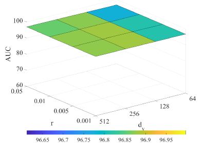
(a) Testing ratio = 10%

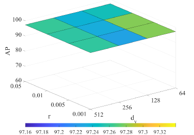
(b) Testing ratio = 10%

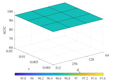
(c) Testing ratio = 20%

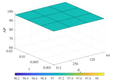
(d) Testing ratio = 20%

Figure 2: The AUC and AP values yielded by the CGCL method with different combinations of $d_{v}$ and $r$ on the Cora dataset.

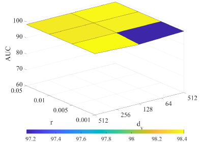
(a) Testing ratio = 10%

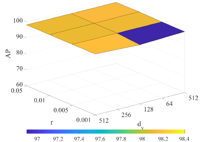
(b) Testing ratio = 10%

(c) Testing ratio = 20%

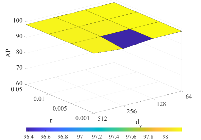
(d) Testing ratio = 20%

Figure 3: The AUC and AP values yielded by the CGCL method with different combinations of $d_{v}$ and $r$ on the Computers dataset.

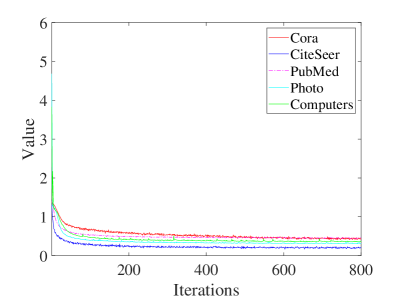
(a) Testing ratio = 10%

(b) Testing ratio = 20%

Figure 4: Convergence results obtained by the CGCL method on all the datasets.

IV-E Training Analysis

We investigate the convergence of the CGCL method. To validate the convergence of the CGCL method, we compute the results of the loss function in Eq. (9) during the training stage. Fig. 4 shows the curves of the loss function results obtained with two different testing ratios on all the datasets. The values of the loss function in Eq. (9) decline sharply in the first few iterations and then decrease gradually until convergence is achieved during the training stage. This offers a further empirical validation of Lemma 1. These observations confirm the robust convergence properties of the CGCL method.

V Conclusion

In this paper, we present a CGCL method that learns invariant graph representations from graph-structured data. CGCL utilizes a bidirectional graph structure augmentation scheme to construct two complementary augmented graph structure views. This augmentation scheme supports graph consistency learning, thereby enhancing the generalizability of the graph representations produced by CGCL. Through cross-view graph consistency learning, CGCL effectively acquires invariant graph representations and facilitates the construction of an incomplete graph structure. Extensive experimental results obtained on graph datasets demonstrate that the proposed CGCL method almost outperforms several state-of-the-art approaches.

References

- [1] J. Chen, H. Mao, D. Peng, C. Zhang, and X. Peng. Multiview clustering by consensus spectral rotation fusion. IEEE Trans. Image Process., pages 5153–5166, 2023a.
- [2] J. Chen, H. Mao, W. L. Woo, , and X. Peng. Deep multiview clustering by contrasting cluster assignments. In Proc. 19th IEEE Int. Conf. Comput. Vis., pages 16752–16761, Paris, France, 2023b.
- [3] J. Chen, Z. Wang, H. Mao, and X. Peng. Low-rank tensor learning for incomplete multiview clustering. IEEE Trans. Knowl. Data Eng., pages 11556–11569, 2023c.
- [4] T. M. Cover and J. A. Thomas. Elements of information theory, 2nd edition. In Wiley, 2006.
- [5] G. Cui, J. Zhou, C. Yang, and Z. Liu. Adaptive graph encoder for attributed graph embedding. In Proc. 26th ACM SIGKDD Int. Conf. Knowl. Discov. Data Min., pages 976–985, 2020.
- [6] W. Hamilton, Z. Ying, and J. Leskovec. Inductive representation learning on large graphs. In Proc. 31th Adv. Neural Inf. Process. Syst., pages 1–11, Long Beach, CA, USA, 2017.
- [7] K. Hassani and A. H. Khasahmadi. Contrastive multi-view representation learning on graphs. In Proc. 37th Int. Conf. Mach. Learn., pages 4116–4126, 2020a.
- [8] K. Hassani and A. H. Khasahmadi. Contrastive multi-view representation learning on graphs. In Proc. 37th Int. Conf. Mach. Learn., pages 4116–4126, 2020b.
- [9] Z. Hou, X. Liu, Y. Cen, Y. Dong, H. Yang, and C. Wang. GraphMAE: Self-supervised masked graph autoencoders. In Proc. 26th ACM SIGKDD Int. Conf. Knowl. Discov. Data Min., pages 976–985, 594-604.
- [10] T. N. Kipf and M. Welling. Variational graph auto-encoders. arXiv preprint, pages 1–3, 2016.
- [11] T. N. Kipf and M. Welling. Semi-supervised classification with graph convolutional networks. In Proc. 5th Int. Conf. Learn. Represent., pages 1–14, Toulon, France, 2017.
- [12] J. Li, R. Wu, W. Sun, S. Tian L. Chen, L. Zhu, C. Meng, Z. Zheng, and W. Wang. What’s behind the mask: understanding masked graph modeling for graph autoencoders. arXiv preprint, pages 1–13, 2022a.
- [13] Y. Li, M. Yang, D. Peng, T. Li, J. Huang, and X. Peng. Twin contrastive learning for online clustering. Int. J. Comput. Vis., 130:2205–2221, 2022b.
- [14] X. Liu, R. Wang, J. Zhou, C. L. P. Chen, T. Zhang, Y. Chen, S. Han, T. Du, K. Ji, and K. Zhang. Transfer learning-based collaborative multiview clustering. IEEE Trans. Fuzzy Syst., 31:1163–1177, 2023a.
- [15] Y. Liu, M. Jin, S. Pan, C. Zhou, Y. Zheng, F. Xia, and P. S. Yu. Graph self-supervised learning: A survey. IEEE Trans. Knowl. Data Eng., 35:5879–5900, 2023b.
- [16] P. Louis, S. A. Jacob, and A. Salehi-Abari. Simplifying subgraph representation learning for scalable link prediction. arXiv preprint, pages 1–9, 2023.
- [17] J. McAuley, C. Targett, Q. Shi, and A. Hengel. Image-based recommendations on styles and substitutes. In Proc. 38th Int. ACM SIGIR Conf. R. D. Inf. Retr., pages 43–52, 2015.
- [18] G. Namata, B. London, L. Getoor, and B. Huang. Query-driven active surveying for collective classification. In 10th Int. WS. Min. Learn. Graphs, pages 43–52, 2012.
- [19] X. Peng, Y. Li, I. W. Tsang, J. Lv H. Zhu, and J. T. Zhou. XAI beyond classification: interpretable neural clustering. J. Mach. Learn. Res., 23(6):1–28, 2022.
- [20] P. Sen, G. Namata, M. Bilgic, L. Getoor, B. Galligher, and T. Eliassi-Rad. Collective classification in network data. AI magazine, 29:93–93, 2008.
- [21] Q. Tan, N. Liu, X. Huang, S. Choi, L. Li, R. Chen, and X. Hu. S2gae: self-supervised graph autoencoders are generalizable learners with graph masking. In Proc. 16th Int. Conf. Web Search Data Min., pages 787–795, Singapore, 2023.
- [22] Y. Tian, C. Sun, B. Poole, D. Krishnan, C. Schmid, and P. Isola. Graph contrastive learning with augmentations. In Proc. 34th Adv. Neural Inf. Process. Syst., pages 6827–6839, Vancouver, BC, Canada, 2020.
- [23] Y. Tsai, H. Zhao, M. Yamada, L. Morency, and R. Salakhutdinov. Neural methods for point-wise dependency estimation. In Proc. 34th Adv. Neural Inf. Process. Syst., pages 62–72, Online, 2020.
- [24] P. Veličkovi’c, G. Cucurull, A. Casanova, A. Romero, P. Li.o, and Y. Bengio. Graph attention networks. In Proc. 6th Int. Conf. Learn. Represent., pages 1–12, Vancouver, BC, Canada, 2018.
- [25] H. Wang, X. Guo, Z. Deng, and Y. Lu. Rethinking minimal sufficient representation in contrastive learning. In Proc. IEEE Conf. Comput. Vis. Pattern Recognit., pages 16041–16050, New Orleans, Louisiana, USA, 2022.
- [26] Y. Wang, S. Han, J. Zhou, L. Chen, C.L. P. Chen, T. Zhang, Z. Liu, L. Wang, and Y. Chen. Random feature based collaborative kernel fuzzy clustering for distributed peer-to-peer networks. IEEE Trans. Fuzzy Syst., 31:692–706, 2023.
- [27] J. Wu, X. Wang, F. Feng, X. He, L. Chen, J. Lian, and X. Xie. Self-supervised graph learning for recommendation. In Proc. 44th Int. ACM SIGIR Conf. R. D. Inf. Retr., pages 726–735, 2021.
- [28] Y. You, T. Chen, Y. Sui Y, T. Chen, Z. Wang, and Y. Shen. Graph contrastive learning with augmentations. In Proc. 34th Adv. Neural Inf. Process. Syst., pages 5812–5823, Online, 2020.
- [29] M. Zhang, P. Li, Y. Xia, K. Wang, and L. Jin. Labeling trick: A theory of using graph neural networks for multi-node representation learning. In Proc. 35th Adv. Neural Inf. Process. Syst., pages 9061–9073, Online, 2021.
- [30] Y. Zhu, Y. Xu, F. Yu adn Q. Liu, S. Wu, and L. Wang. Deep graph contrastive representation learning. arXiv preprint, pages 1–9, 2020.