Spectroscopy of elementary excitations from quench dynamics in a dipolar XY Rydberg simulator

Abstract

We use a Rydberg quantum simulator to demonstrate a new form of spectroscopy, called quench spectroscopy, which probes the low-energy excitations of a many-body system. We illustrate the method on a two-dimensional simulation of the spin-1/2 dipolar XY model. Through microscopic measurements of the spatial spin correlation dynamics following a quench, we extract the dispersion relation of the elementary excitations for both ferro- and anti-ferromagnetic couplings. We observe qualitatively different behaviors between the two cases that result from the long-range nature of the interactions, and the frustration inherent in the antiferromagnet. In particular, the ferromagnet exhibits elementary excitations behaving as linear spin waves. In the anti-ferromagnet, spin waves appear to decay, suggesting the presence of strong nonlinearities. Our demonstration highlights the importance of power-law interactions on the excitation spectrum of a many-body system.

The nature and spectrum of elementary excitations are defining features of quantum matter. They reflect low-energy physics, and dictate how quantum information propagates in the system [1, 2, 3]. These elementary excitations are often waves characterized by a dispersion relation $\omega_{\bm{k}}$ that connects their energy to their wavevector $\bm{k}$. This relation depends on the dimensionality of the system, its symmetries, and the range of the interactions between particles. Excitations are traditionally probed in condensed matter via linear response, which relies on cooling the system down to low temperatures and measuring its equilibrium response to weak perturbations [4, 5, 6, 7]. The ability offered by synthetic quantum systems to monitor (nearly) unitary evolution, in both space and time, provides an alternative approach to probe the excitations: one can inject a finite density of excitations into the system and observe the subsequent dynamics – a so-called quench experiment [8]. Following the quench, the re-organization of spatial correlations is then dictated by the propagation of excitations, which is governed by their dispersion relation. This intuition can be put on firm ground when the elementary excitations are free quasi-particles: in that case, the Fourier transform of the equal time correlations in space at wavevector ${\bm{k}}$ – hereafter termed the time-dependent structure factor (TSF) – is expected to oscillate in time at frequency $2\omega_{\bm{k}}$ [9, 10, 11, 12, 13]. This result forms the basis of quench spectroscopy, which we implement here.

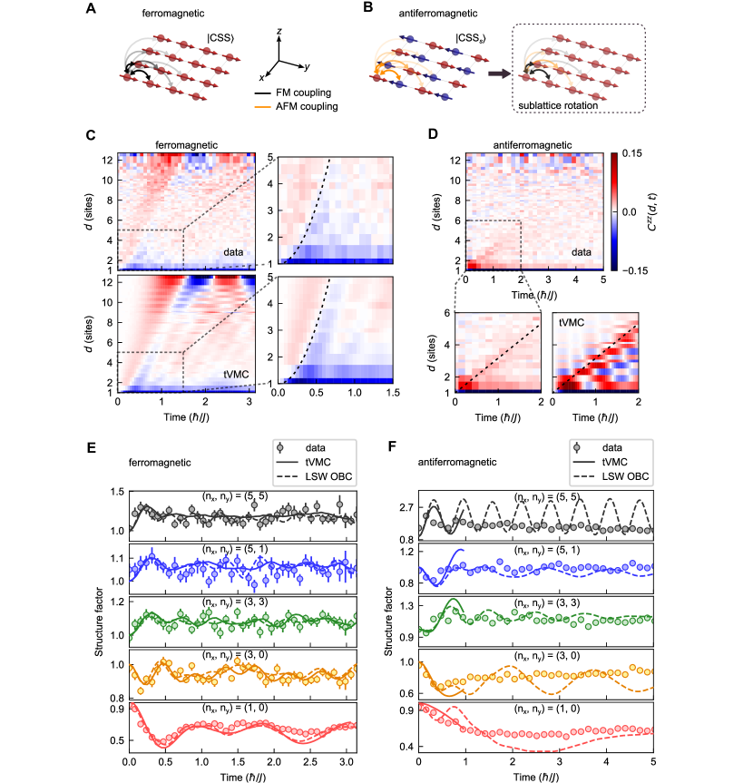
Figure 1: Quench spectroscopy of the 2$d$ dipolar XY model. (A) Schematic representation of the classical ferromagnetic state along $y$ prepared during the quench, $|{\rm CSS}\rangle=\left|\rightarrow\cdots\rightarrow\rightarrow\right\rangle_{y}$, featuring the dipolar FM couplings. (B) Schematic representation of the initial classical antiferromagnetic state along $y$, $|{\rm CSS}_{s}\rangle=\left|\leftarrow\rightarrow\cdots\rightarrow\leftarrow\right\rangle_{y}$, featuring the dipolar AFM couplings. Applying a canonical transformation $\sigma_{i}^{x(y)}\to(-1)^{i}\sigma_{i}^{x(y)}$ on the spins of one of the two sublattice of the AFM state transforms it into a FM CSS state with frustrated couplings (see text). (C),(D) Space-time dynamics of the spin correlations following the quench into the coherent spin state $|{\rm CSS}\rangle$ (FM case, (C)) or the staggered coherent spin state state $|{\rm CSS}_{s}\rangle$ (AFM case, (D)). The dashed line in (C) is a guide to the eye $d\sim t^{2}$. The one in (D) corresponds to $d\approx 2v_{g}t/a$, with $v_{g}$ extracted from the dispersion relation (Fig. 2B). (E),(F) Time evolution of the FM and AFM structure factors $S(k_{x},k_{y},t)$ (with $(k_{x},k_{y})=(2\pi/L)(n_{x},n_{y})$) extracted from the data in (C) and (D) (circles). The error bars represent $68\%$ confidence intervals. Solid lines: results of tVMC simulation. Dashed lines: results of LSW spin-wave theory including the experimentally-calibrated state detection errors. the AFM, we show in (F) the results of tVMC only for $t\lesssim\hbar/J$ as the results are not quantitatively accurate for later times (see [14]).

Our experiment employs a Rydberg-atom quantum simulator, consisting of a two-dimensional square array of $N=L\times L=10\times 10$ ⁸⁷Rb atoms trapped in optical tweezers (see Fig. 1A). We encode the pseudo spin-1/2 using a pair of Rydberg states $\left|\uparrow\right\rangle=|60S_{1/2},m_{j}=1/2\rangle$ and $\left|\downarrow\right\rangle=|60P_{3/2},m_{j}=-1/2\rangle$, which are coupled by resonant dipole-dipole exchange between the atoms  [15, 14]. The system is well-described by the dipolar XY Hamiltonian,

$$H_{\rm XY}=-{\frac{J}{2}}\sum_{i<j}\frac{a^{3}}{r_{ij}^{3}}(\sigma^{x}_{i}\sigma^{x}_{j}+\sigma^{y}_{i}\sigma^{y}_{j}),$$ (1)

where $J/h=0.25\leavevmode\nobreak\$MHz is the dipolar interaction strength, $\sigma_{i}^{x,y,z}$ are Pauli matrices, $r_{ij}$ is the distance between spins $i$ and $j$, and $a=15\leavevmode\nobreak\ \mu$m is the lattice spacing. We apply a magnetic field perpendicular to the lattice plane to define the quantization axis and ensure isotropic dipolar interactions. After initializing the system in an uncorrelated product state, corresponding to the mean-field (MF) ground-state for ferromagnetic (FM) or antiferromagnetic (AFM) interactions, we then monitor the evolution of equal-time spin correlations in real space, as well as in momentum space by evaluating the TSF. Our main results are twofold. In the case of FM dipolar interactions, the excitations are found to behave as long-lived spin waves (also called magnons), whose frequency can be extracted from the persistent oscillations of the TSF. We observe the characteristic non-linear dispersion relation of dipolar spin waves in two spatial dimensions, predicted to scale as $\omega_{\bm{k}}\sim\sqrt{k}$ for small $k$ [16]. For AFM interactions, a different picture emerges. There, the frustrated nature of the antiferromagnetic dipolar interactions leads to a linear dispersion relation at small wavevectors. Moreover, the oscillations of the AFM TSF are strongly damped, suggesting the existence of decay processes which render spin waves unstable.

We begin the quench spectroscopy protocol by preparing either a uniform coherent spin state (CSS) $|{\rm CSS}\rangle=\left|\rightarrow\cdots\rightarrow\rightarrow\right\rangle_{y}$ aligned along the $y$ axis, or a staggered CSS $|{\rm CSS}_{s}\rangle=\left|\leftarrow\rightarrow\cdots\rightarrow\leftarrow\right\rangle_{y}$ (Fig. 1A,B). The uniform CSS is the MF ground state of the FM dipolar XY Hamiltonian $H_{\rm XY}$, and its dynamical evolution is thus governed by the low-energy excitations above the true ground state. The staggered CSS, on the other hand, is the MF ground state for AFM interactions, namely for $-H_{\rm XY}$. Due to time-reversal symmetry, the ensuing evolution can be viewed as low-energy dynamics governed by the AFM dipolar XY Hamiltonian $-H_{\rm XY}$ [10]. To clarify the contrast between the two cases, we apply a canonical transformation in the AFM case, rotating spins on one sublattice by $\pi$ around the $z$-axis, so that $\sigma_{i}^{x(y)}\to(-1)^{i}\sigma_{i}^{x(y)}$. In this relabeled coordinate system, the initial state becomes the same for the FM and the AFM, but the Hamiltonian of the AFM transforms into that of a frustrated ferromagnet with staggered couplings, $(Ja^{3}/r_{ij}^{3})(-1)^{i+j+1}$ (Fig. 1B).

After a given evolution time $t$, we read out the state of each atom [17, 18] in the $z$-basis, and reconstruct the equal time correlation function for the $z$ spin components of the atom pair $(i,j)$, $C^{zz}_{ij}(t)=\langle\sigma^{z}_{i}\sigma^{z}_{j}\rangle(t)-\langle\sigma^{z}_{i}\rangle(t)\langle\sigma^{z}_{j}\rangle(t)$. The choice of the $z$ basis is dictated by the fact that $\sigma^{z}$-operators correspond to spin flips in the $xy$ plane, thus revealing excitations above low-energy states which exhibit long-range order for the $x$ and $y$ spin components [14]. The space-time evolution of the correlations is presented in Fig. 1(D,E), where we show the correlation function averaged over all $N_{d}$ pairs of spins separated by the same distance $d$, $C^{zz}(d,t)=N_{d}^{-1}\sum_{ij|r_{ij}=d}C^{zz}_{ij}(t)$. Strikingly, the correlations differ between the FM and the AFM at both short and long distances. At short distances, the correlations are negative in the FM, while they alternate in sign (and are stronger) in the AFM – a subtle effect that we discuss at the end of this paper. Moreover, the correlations of the FM propagate rapidly in space and reach the longest-distances in less than an interaction time $\hbar/J$. The data are also consistent with the super-ballistic propagation of correlation fringes predicted to scale as $d\sim t^{2}$ for the dipolar XY model [10]. This is highlighted by the dotted line in Fig. 1D. In the AFM, we find that the correlations propagate slower, and that the correlation front moves linearly with time (dotted line in Fig. 1E). This difference is due to frustration, which effectively shortens the range of the interaction and leads to a finite maximal group velocity $v_{g}=\max_{\bm{k}}|\nabla_{\bm{k}}\omega_{\bm{k}}|\approx Ja/\hbar$ of the elementary excitations, such that $d\approx 2v_{g}t/a$ [3]. Moreover, the correlations appear to vanish at a finite distance of $\sim$ 6 sites, a consequence of thermalization towards a state with short-range correlations (see below).

Figure 2: Measurement of the dispersion relation of the dipolar XY model. (A),(B) Frequency $\omega_{\bm{k}}$ as a function of $|{\bm{k}}|=\sqrt{k_{x}^{2}+k_{y}^{2}}$, fitted from the time-dependent structure factors shown in Fig. 1F,G. The ferromagnetic case (A) exhibits a non-linear dispersion relation. The antiferromagnetic case (B) shows a linear dispersion relation. (C),(D) Frequencies $\omega_{\bm{k}}$ obtained by using Eq. (3) and the fitted offset of $S(\bm{k},t)$. The data (filled circles) are compared to the results of LSW with, PBC (open circles), mPBC (square) and tVMC (diamonds), see text. On all figures, the error bar represents the standard error from the fits.

The TSF is then obtained by Fourier transforming the correlation function at equal time:

$$S(\bm{k},t)=(1/N)\sum_{i,j}e^{i{\bm{k}}\cdot{\bm{r}}_{ij}}C^{zz}_{ij}(t),$$ (2)

with wave-vectors $\bm{k}=(2\pi/L)(n_{x},n_{y})$ where $n_{x(y)}=-L/2+1,...,L/2$. As observed in Fig. 1E,F, the TSF exhibits oscillations at short times for all wavevectors (full data set in [14]). In the FM case, the oscillations persist at longer times for small wave-vectors. The oscillations in the AFM case have a lower frequency than their FM counterpart at the same wavevector, and appear damped at long times. In both cases, we compare the experimental data with the predictions of linear spin-wave (LSW) theory and with time-dependent variational Monte Carlo (tVMC) (see details in [14]). In the FM case, we observe good agreement between the experimental results and both theoretical predictions (which also agree with one another), suggesting that the elementary excitations of the FM behave as undamped, linear spin waves. Contrarily, the AFM data are in rather poor agreement with LSW theory, which does not predict any damping – thus suggesting that the AFM dynamics is strongly non-linear.

We then extract the dispersion relation $\omega_{\bm{k}}$ of elementary excitations from a fit of $S(\bm{k},t)$ to the form $A_{\bm{k}}\cos(2\omega_{\bm{k}}t+\phi_{\bm{k}})+C_{\bm{k}}$, predicted by LSW theory. Although our system lacks well-defined wavevectors due to its open boundary conditions (OBC), this fit is still applicable because its early-time dynamics is approximately equivalent to that of a system with periodic boundary conditions and modified couplings (mPBC), as we detail in the Method [14]. We thus restrict the fits to early times, i.e. to the data points of the first full oscillation. In Fig. 2, we show the dispersion relation $\omega_{\bm{k}}$ extracted from fits to the experimental data and to the tVMC simulation, and also compare to the predictions of LSW [10]. Namely, for dipolar XY systems with mPBC, one expects $\hbar\omega_{\bm{k}}/J=\gamma_{0}\sqrt{1-\gamma_{\bm{k}}/\gamma_{0}}$, where $\gamma_{\bm{k}}=(1/N)\sum_{i\neq j}e^{i{\bm{k}}\cdot{\bm{r}}_{ij}}\eta^{i+j+1}a^{3}/r_{ij}^{3}$ with $\eta=1(-1)$ for the FM (AFM). In the FM case, we observe a non-linear dispersion down to the smallest wavevector – in agreement with the LSW prediction that $\omega_{\bm{k}}\sim\sqrt{k}$ as $k\to 0$ due to the long-range dipolar tail [16, 10]. Also, LSW theory with mPBC matches the experiment rather accurately. For the AFM, we instead obtain a linear dispersion relation at small $k$ (and even beyond) from both the experimental and tVMC data, characteristic of effective short-range interactions [19]. This is in agreement with the light-cone picture of correlation spreading in real space seen in Fig. 1, with a spin-wave velocity $v_{g}\approx Ja/\hbar$. Again, the experimental and tVMC fits agree well with the LSW prediction, which therefore suggests that the linearized theory correctly captures the frequency of elementary excitations. However, it does not predict their observed decay in the AFM.

As is evident in Fig. 2A, the fit-extracted frequencies exhibit a significant spread. This arises from the difficulty of reliably fitting small-amplitude oscillations, especially for $ka\approx\pi$. This calls for a second method to extract the frequency. Fortunately, LSW theory predicts a relationship between the offset $C_{\bm{k}}$ and the frequency $\omega_{\bm{k}}$ [10]:

$$\hbar\omega_{\bm{k}}=J\gamma_{0}\sqrt{2C_{\bm{k}}-1}\ ,$$ (3)

where $\gamma_{0}^{\textrm{FM}}\approx 6.5$ and $\gamma_{0}^{\textrm{AFM}}\approx 2.5$ for our $10\times 10$ array. Working under the assumption that the excitations are indeed linear spin waves, we extract $C_{\bm{k}}$ from a fit to the data shown in Fig. 1F,G, and infer $\omega_{\bm{k}}$ using Eq. (3). The thus-inferred dispersion relation is shown in Fig. 2C,D, for both the experimental and tVMC data. We also compare to the predictions of LSW theory for a system with mPBC. In the FM, we observe excellent agreement, which again confirms the validity of LSW theory for this system. The AFM also shows rather good agreement, despite the fact that its state preparation is plagued with more imperfections than the FM, and that its spin waves are not expected to be stable, as we discuss below.

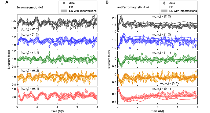
Figure 3: Time evolution of the structure factors $S(k_{x},k_{y},t)$ for a 4$\times$4 array. The black solid lines are the results of exact diagonalization simulations, without or with experimental imperfections. (A),(B) ferromagnetic and antiferromagnetic case, respectively.

We now address the long-time dynamics, which, as previously noted, differs for the FM and AFM. First, to assess whether the decay observed in Fig. 1G for the AFM dynamics is due to experimental imperfections, or if it is intrinsic to the unitary dynamics of the system, we scale our experiment down to $N=4\times 4$ atoms, which can be exactly simulated, including all the known experimental imperfections (details of imperfections in SM [14]). The results are presented in Fig. 3A,B. In both the FM and the AFM, we observe that the experimental imperfections do not fundamentally alter the dynamics at long times. This suggests that the decay of oscillations in the AFM is indeed intrinsic, which may be attributed to an instability of the spin-wave excitations. As we further elaborate in the SM [14], the origin of this instability can be attributed to several effects. The first non-linear correction to the AFM spin-wave theory predicts a decay of single magnons into three magnons of lower energy and momentum. This decay is instead negligible for the FM, due to kinematical constraints on magnon decay that lead to a lack of phase space for the decay process. Moreover, as revealed by a systematic study of different spectral functions (see [14]), the decay must also come from multi-magnon processes resulting from the finite density of magnons injected into the system during the initial state preparation.

Second, we discuss the issue of thermalization at long times. For both the FM and the AFM, one could expect equilibration of local observables to thermal equilibrium at a temperature $T_{\rm CSS}$ corresponding to the energy of the initial state, namely such that $\langle H_{\rm XY}\rangle_{T_{\rm CSS}}=\langle{\rm CSS}|H_{\rm XY}|{\rm CSS}\rangle$. Experimentally, after the short initial transient from which we extract the dispersion relation, the TSF tends to oscillate around a well-defined value, which can be interpreted as signaling the onset of equilibration. Assuming the eigenstate-thermalization hypothesis [20], these oscillations should take place around the thermal-equilibrium value of the TSF at $T_{\rm CSS}$, with an amplitude decreasing exponentially with system size. In the FM, however, this prediction should be taken with some caution, as the dynamics of linear spin waves has an effectively integrable nature. As such, it cannot lead to proper thermalization, but only to dephasing (or pre-thermalization [21]) when looking at quantities which probe several spin-wave frequencies. For the AFM, instead, the damping of oscillations suggests a fully chaotic dynamics and proper thermalization.

For both the FM and AFM we extract the equilibrium value of the TSF by averaging the data after the initial transient of duration $\hbar/J$. The resulting time-averaged structure factors $\mathrm{bar}{S}(\bm{k})$ are shown in Fig. 4. For the FM, we calculate the thermalized structure factor via equilibrium quantum Monte Carlo (QMC) [14] (accounting also for the conservation of structure factor at $k=0$). We find that this value is in excellent agreement with the one averaged over the oscillations, indicating that the pre-thermalized structure factor coincides with the thermal one. The corresponding temperature is $T_{\rm CSS}^{\rm FM}\approx 1.2J/k_{\rm B}$, lying deep inside the long-range ordered regime [22, 14] where spin waves should be the dominant thermally populated excitations. We also find that their density remains small (see SM [14]), justifying the picture of linear dynamics.

In the AFM case, predicting the thermal value for the TSF is challenging due to the sign problem in QMC. Using tensor network methods, we estimate that $T_{\rm CSS}^{\rm AFM}\approx 0.6J/k_{\rm B}$, falling in a paramagnetic phase above a Berezinskii-Kosterlitz-Thouless transition [17, 14]. In this regime, non-linear excitations (including unbound vortex-antivortex pairs) should be thermally populated. This is reflected by a significantly higher density of spin waves developed during the dynamics [14], which implies non-linearities play a prominent role. Nonetheless, we again observe a relatively good agreement between the experimental data and the predictions of tVMC and LSW theory. For comparison, we also plot the results of an equilibrium QMC calculation for the XY model with nearest-neighbor interactions, at the corresponding $T_{\rm CSS}$ for that model. The agreement with the experimental data is unexpectedly good, suggesting again the effective short-range nature of the frustrated dipolar interactions.

Both the FM and the AFM show a peak of $\mathrm{bar}{S}(\bm{k})$ at ${\bm{k}}a=(\pi,\pi)$, reflecting the short-range anti-correlations that we observed in Fig. 1D,E. To understand the structure of these correlations emerging at long times, we map the dipolar spin-1/2 XY model onto hardcore bosons [23]: the anti-correlations in the $\sigma^{z}$ spin components reflects the tendency of hardcore bosons to form staggered density patterns for which the dipolar hoppings allow them to delocalize and reduce their kinetic energy. This has been observed in one-dimensional repulsive bosonic gases, leading to short-range crystallization [24]. Surprisingly the frustrated hoppings of the AFM case appear to lead to significantly stronger correlations (namely, a higher peak) than the unfrustrated, FM ones. This behavior is opposite to what happens to phase correlations – namely the correlations among the $\sigma^{x(y)}$ spin components – which thermalize to long-range order in the FM case, while they are expected to thermalize to short-range order in the AFM case due to frustration [17]. This enhancement of $\sigma^{z}$ correlations by frustrating the ordering of the $\sigma^{x(y)}$ components can be understood as a result of the effective hopping range in the corresponding bosonic model: In the FM case, bosons delocalize and correlate in phase over all distances thanks to the dipolar hopping, so that short-range density correlations are weakened; contrarily, in the AFM case, bosons delocalize only at short range because of the frustrated hopping, and they do so by enhancing (short-range) density correlations.

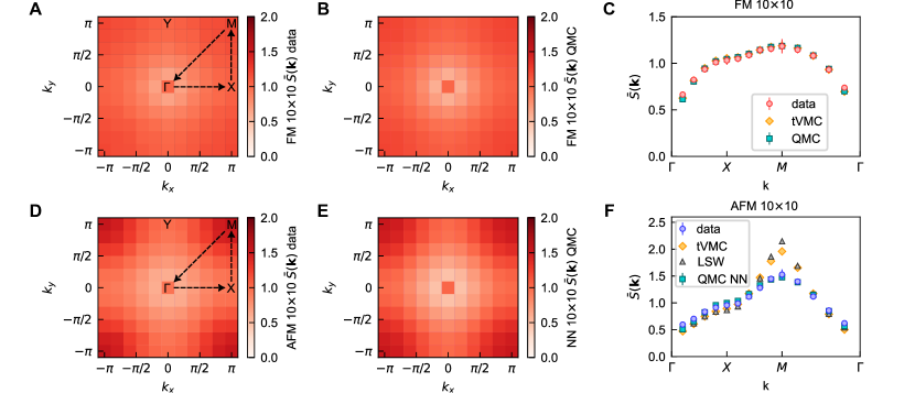
Figure 4: Time-averaged structure factor $\mathrm{bar}{S}(\bm{k})$. (A),(B)((D),(E) Comparison of experimental data and Quantum Monte Carlo (tVMC) simulations for the ferromagnetic (antiferromagnetic) case, plotted in the first Brillouin zone. (C),(F) Experimental time-average structure factor $\mathrm{bar}{S}(\bm{k})$ plotted along the path connecting the high symmetry points of the Brillouin zone (dotted lines in (A),(D)). We also plot the predictions from tVMC, Quantum Monte Carlo (FM case), LSW (AFM) and QMC with nearest-neighbor (NN) interactions (AFM).

In conclusion, we have experimentally reconstructed the dispersion relation of a strongly interacting quantum system (the 2$d$ quantum dipolar XY model) using quench spectroscopy. Our results highlight the special role of ferromagnetic dipolar interactions in two dimensions, whose long-range tail leads to a non-linear dispersion relation of excitations with unbounded maximal group velocity, accelerating the dynamics with respect to finite-range interactions. The frustration resulting from the antiferromagnetic dipolar interactions leads instead to an effective cancellation of the long-range tail, recovering a linear dispersion relation as in the case of finite-range interactions. We observe that the elementary excitations of the dipolar ferromagnet have the nature of linear spin waves, leading to effectively integrable dynamics at low energy. On the contrary, the dipolar antiferromagnet shows a decay of spin-wave oscillations, highlighting the importance of non-linear quantum fluctuations in the system. Similar spectroscopic analyses have been applied to the evolution of quantum simulators after the application of a local perturbation starting from the ground state [25], or of a parametric perturbation at a given wavevector [26, 27]. Our approach is instead based on a global uniform quench, akin to that adopted in previous experiments on dilute Bose gases [28, 29] and trapped ion chains [30]. It relies only on the initialization of the system in the mean-field ground state of the Hamiltonian, in order to target the low-energy spectrum. Our procedure can be extended by using different initial states in order to address higher-energy regions of the excitation spectrum. It could also be applied to more exotic phases of matter, such as magnetism on frustrated triangular or kagomé lattices, supporting strongly fluctuating ordered phases or perhaps even fractionalized spin liquids [31].

Supplemental Material

I Experimental methods

I.1 Experimental procedures

The implementation of the dipolar XY Hamiltonian is based on the ${}^{87}\text{Rb}$ Rydberg-atom tweezer array platform described in previous works [17, 18]. The pseudo spin-states $\ket{\uparrow}=\ket{60S_{1/2},m_{J}=1/2}$ and $\ket{\downarrow}=\ket{60P_{3/2},m_{J}=-1/2}$ can be coupled by microwave at 17.2 GHz (see Fig. S1A). To isolate the $\ket{\uparrow}-\ket{\downarrow}$ transition from irrelevant Zeeman sublevels we apply a $\sim 45$-G quantization magnetic field perpendicular to the array.

Experimental sequence (Fig. S1) – We assemble arrays of atoms trapped in 1-mK deep optical tweezers [32], Raman sideband cool them down to $10\,\mu$K and optically pump them into $\ket{g}=\ket{5S_{1/2},F=2,m_{F}=2}$. We then adiabatically reduce the trap depth by a factor $\sim 50$ to further reduce the temperature. The tweezers are finally switched off and the atoms are excited to the Rydberg state $\ket{\uparrow}$ by a stimulated Raman adiabatic passage (STIRAP) with 421-nm and 1013-nm lasers.

To initialize the atoms in $|{\rm CSS}\rangle=\ket{\rightarrow\cdots\rightarrow}$ (FM case), we apply a global resonant microwave $\pi/2$ pulse around $x$, with a Rabi frequency $\Omega=2\pi\times 22.2$ MHz (Fig. S1B). For the AFM case, we need to initialize the system in $|{\rm CSS}_{s}\rangle=\left|\leftarrow\rightarrow\cdots\rightarrow\leftarrow\right\rangle_{y}$. As the microwave field does not allow for local manipulations, we combine them with local addressing laser beams and use the following procedure. We first apply a global resonant microwave $\pi$ pulse around $x$ transferring all the spins from $\ket{\uparrow}$ to $\ket{\downarrow}$, (Fig. S1C). We then apply a staggered addressing light-shift ($\sim 11$ MHz) on half of the atoms and, simultaneously, a weaker microwave $\pi$-pulse ($\Omega=2\pi\times 7.7$ MHz) to transfer only the non-addressed atoms back to $\ket{\uparrow}$ while keeping the addressed atoms in $\ket{\downarrow}$. This leads to the AFM state along $z$ $\left|\downarrow\uparrow\cdots\downarrow\uparrow\right\rangle$. Finally, we apply a global resonant microwave $\pi/2$ pulse around $x$ ($\Omega=2\pi\times 22.2$ MHz) to get to the state $|{\rm CSS}_{s}\rangle$.

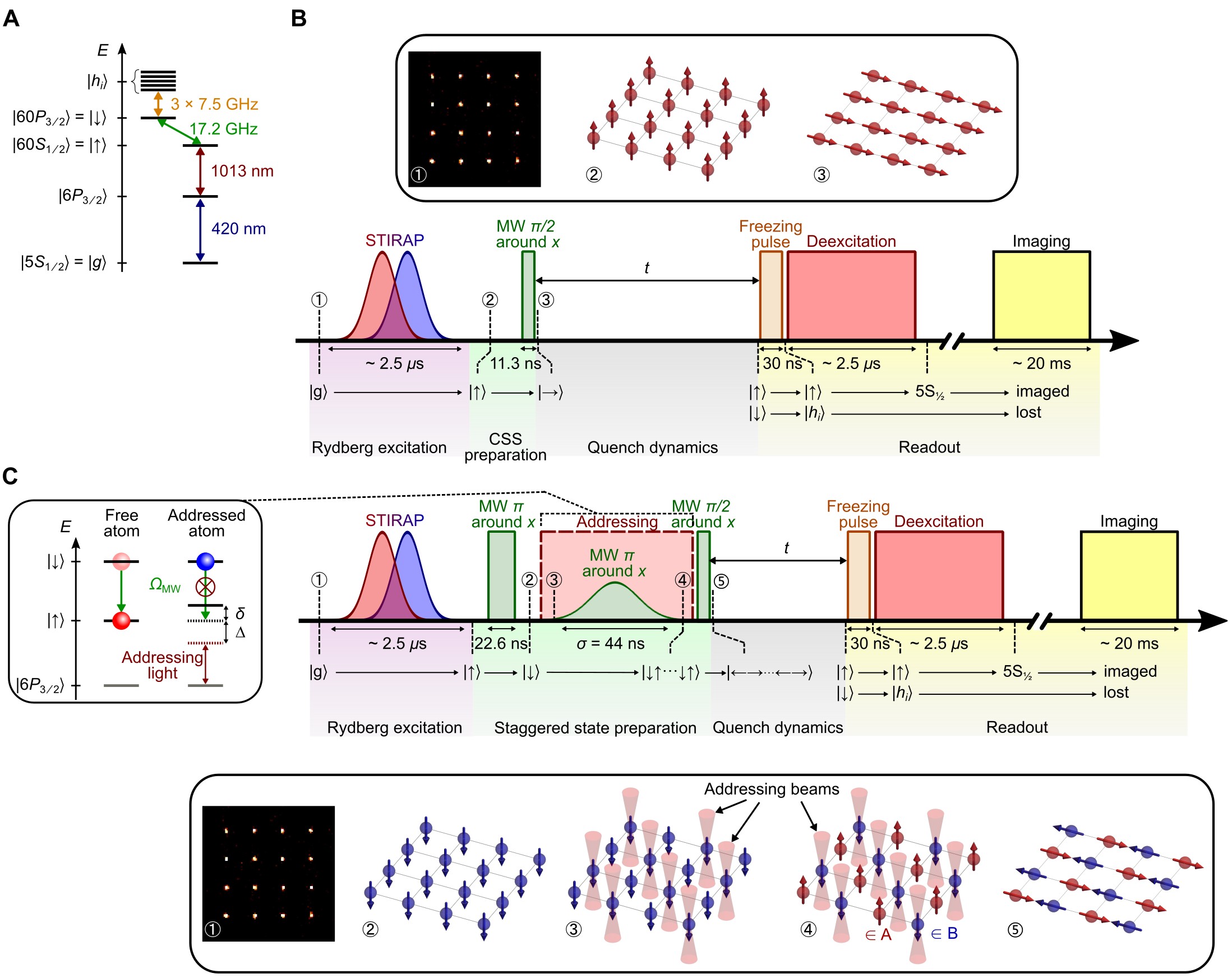
Figure S1: Experimental sequence. (A) Schematics of the atomic levels relevant for the experiment. (B) Sequence of optical and microwave pulses (not to scale) used for the experiments in the ferromagnetic case reported in the main text. (C) Sequence of optical and microwave pulses (not to scale) used for the experiments in the antiferromagnetic case reported in the main text.

State-detection procedure – The detection protocol includes three parts. First, we apply a $7.5\leavevmode\nobreak\$GHz microwave pulse (“freezing pulse” in Fig. S1) to transfer the population from $\ket{\downarrow}$ to the $n=58$ hydrogenic manifold (states $\ket{h_{i}}$ in Fig. S1A). Atoms in the hydrogenic states are decoupled from those in $\ket{\uparrow}$, thus avoiding detrimental effects of interactions during the read-out sequence. Second, a $2.5\leavevmode\nobreak\ \mu$s-deexcitation pulse resonant with the transition between $\ket{\uparrow}$ and the short-lived intermediate state $6P_{3/2}$ leads to decay of the atoms back to $5S_{1/2}$. Third, we switch the tweezers back on to recapture and image (via fluorescence) only the atoms in $5S_{1/2}$ (the others being lost). This protocol maps the $\ket{\uparrow}$ (resp. $\ket{\downarrow}$) state to the presence (resp. absence) of the corresponding atom. The experimental sequence is typically repeated $400$ times with defect-free $4\times 4$ assembled arrays, and $\sim 400$ shots with at most 2 defects allowed in the $10\times 10$ assembled arrays. This allows us to reconstruct the spin correlations and the structure factors by averaging over these repeated measurements.

I.2 Experimental imperfections

Several sources of state preparation and measurement (SPAM) error contribute to affecting the observed structure factors.

State preparation errors – We estimate that the Rydberg excitation process is $98\%$ efficient: a fraction $\eta=2\%$ of the atoms remains in the state $|g\rangle$ after Rydberg excitation and hence do not participate in the dynamics. These uninitialized atoms are read as a spin $\left|\uparrow\right\rangle$ at the end of the sequence. For the FM case, the following $\pi/2$-microwave pulse used to prepare CSS is also imperfect due to the unavoidable effect of the dipolar interactions between the atoms during its application: it reduces the initial polarization by $\sim 1\%$. For the AFM case, the $\pi$-microwave pulse applied simultaneously to the addressing laser has an efficiency $\eta_{\text{non-add}}$ to transfer the non-addressed atoms back to $\ket{\uparrow}$, and $\eta_{\text{add}}$ to transfer the addressed atoms to $\ket{\uparrow}$. For the $4\times 4$ array with $\sim 68\leavevmode\nobreak\$MHz addressing light-shift we find $\eta_{\text{non-add}}=98\%$ and $\eta_{\text{add}}=2\%$. For the $10\times 10$ arrays with $\sim 11\leavevmode\nobreak\$MHz addressing light-shift, we get $\eta_{\text{non-add}}=95\%$ and $\eta_{\text{add}}=2\%$. The fact that $\eta_{\text{add}}$ has the same value in the two cases is fortuitous and indicates that processes other than off-resonant microwave transitions play a role.

Measurement errors – Due to the finite efficiency of each step in the readout sequence (see Fig. I.1B), an atom in $\ket{\uparrow}$ (resp. $\ket{\downarrow}$) has a non-zero probability $\epsilon_{\uparrow}$ (resp. $\epsilon_{\downarrow}$) to be detected in the wrong state [17]. The main contributions to $\epsilon_{\uparrow}$ are the finite efficiency $1-\eta_{\text{dx}}$ of the deexcitation pulse and the probability of loss $\epsilon$ due to collisions with the background gas. As for $\epsilon_{\downarrow}$, the main contribution is the $\ket{\downarrow}$ Rydberg state radiative lifetime. A set of calibrations leads, to first order, to $\epsilon_{\uparrow}\simeq\eta_{\text{dx}}+\epsilon=1.5\%+1.0\%=2.5\%$ and $\epsilon_{\downarrow}=1.0\%$.

The experimental structure factors $S(k_{x},k_{y};t)$ are related to the same quantities $\tilde{S}(k_{x},k_{y};t)$ without detection errors by the following equations (valid to first order in $\epsilon_{\uparrow,\downarrow}$):

$$\begin{split}S(k_{x},k_{y};t)=\leavevmode\nobreak\ &(1-2\epsilon_{\downarrow}-2\epsilon_{\uparrow})\tilde{S}(k_{x},k_{y};t)\\ &+2\epsilon_{\downarrow}+2\epsilon_{\uparrow}.\end{split}$$ (4)

The results of numerical simulations and spin-wave theory shown in the various figures include the detection errors.

II Representative fits of the experimental data for the time-dependent structure factor

Figures S2 (FM case) and S3 (AFM) present full data sets for the time-dependent structure factor $S(k_{x},k_{y};t)$ from the experimental data and the data obtained by tVMC calculations. Both experimental and numerical data are fitted with the same function $A_{\bm{k}}\cos(2\omega_{\bm{k}}t+\phi_{\bm{k}})+C_{\bm{k}}$ during the early dynamics.

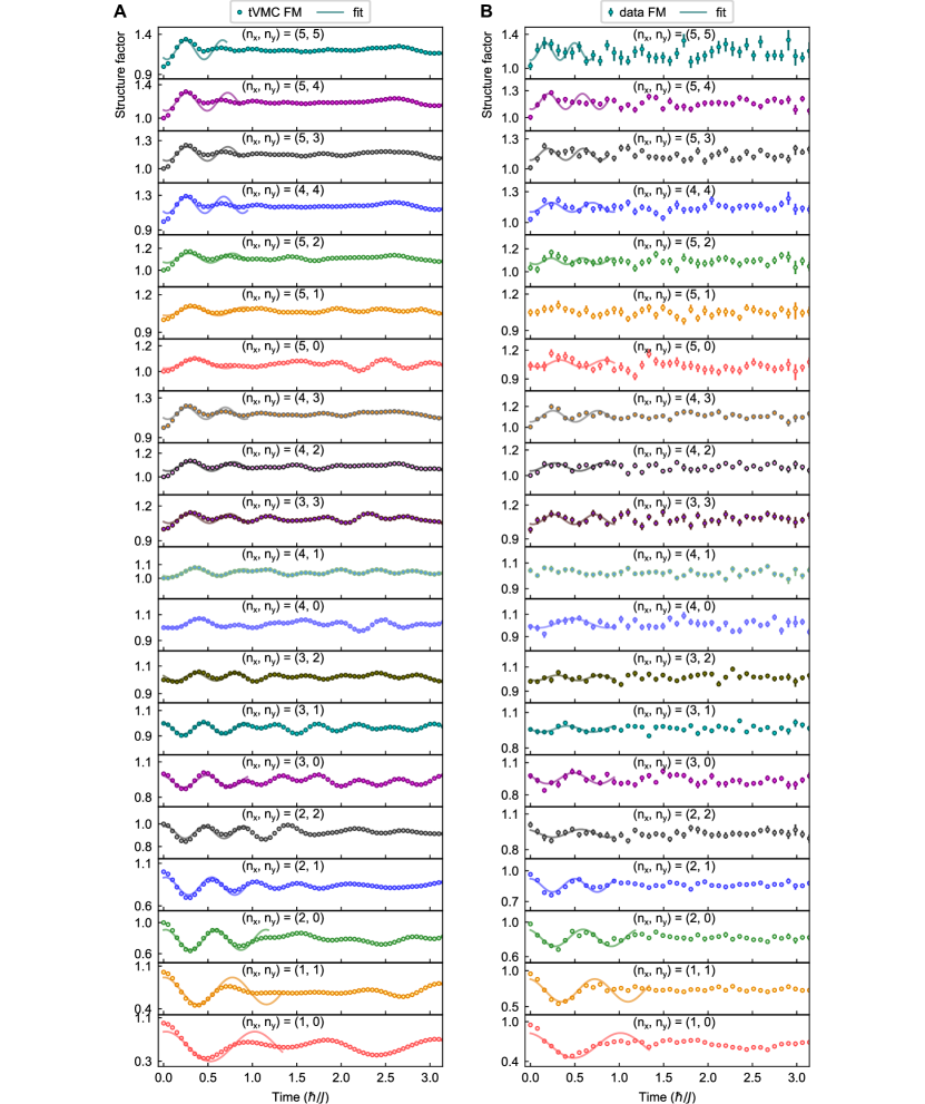
Figure S2: Full data sets for the time-dependent ferromagnetic structure factor $S(k_{x},k_{y};t)$. (Left): tVMC calculations. (Right): experimental data. Line: fit by the function $A_{\bm{k}}\cos(2\omega_{\bm{k}}t+\phi_{\bm{k}})+C_{\bm{k}}$. Here, $(k_{x},k_{y})=(2\pi/L)(n_{x},n_{y})$ where $n_{x(y)}=-L/2+1,...,L/2$. For $(n_{x},n_{y})=(4,1),(5,1)$, the fitting curves are not shown as the standard deviations of the fitting parameter $\hbar\omega_{k}/J$ are very large.

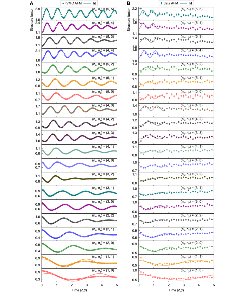
Figure S3: Full data sets for the time-dependent antiferromagnetic structure factor $S(k_{x},k_{y};t)$. (Left): tVMC calculations. (Right): experimental data. Line: fit by the function $A_{\bm{k}}\cos(2\omega_{\bm{k}}t+\phi_{\bm{k}})+C_{\bm{k}}$. Here, $(k_{x},k_{y})=(2\pi/L)(n_{x},n_{y})$ where $n_{x(y)}=-L/2+1,...,L/2$.

III Principle of the quench spectroscopy method

We discuss here the bases of quench spectroscopy (QS) introduced in several works [9, 10, 11, 12, 13], as applied to lattice spin models with periodic boundary conditions. The quantity of interest is the time-dependent structure factor

$$S^{\mu\mu}(\bm{k},t) = \frac{1}{N}\sum_{ij}e^{-i\bm{k}\cdot(\bm{r}_{i}-\bm{r}_{j})}\langle\Psi(t)|\sigma^{\mu}_{i}\sigma^{\mu}_{j}|\Psi(t)\rangle$$ (5)

$$= \langle\Psi(t)|\sigma_{\bm{k}}^{\mu}\sigma_{-\bm{k}}^{\mu}|\Psi(t)\rangle$$

where $\mu=x,y,z$. We have introduced the Fourier transform of the spin operators

$$\sigma_{\bm{k}}^{\mu}=\frac{1}{\sqrt{N}}\sum_{i}e^{-i\bm{k}\cdot\bm{r}_{i}}\sigma_{i}^{\mu}\leavevmode\nobreak\ .$$ (6)

We consider quench experiments which start from a product state $|\Psi(0)\rangle=\otimes_{i=1}^{N}|\psi_{i}\rangle$, corresponding to the mean-field approximation to the ground state of the spin Hamiltonian $H$ of interest. If such a ground state has spins forming a pattern in the $xy$ plane (as is the case in our work), elementary excitations (with integer spin $s=1$) are spin flips with respect to these spin orientations: They are generated locally by the $\sigma_{i}^{z}=(\sigma_{i}^{+}+\sigma_{i}^{-})/2$ operator – $\sigma_{i}^{\pm}$ being the raising/lowering operators of spin $i$ with respect to the $y$ quantization axis, along which the spins are aligned in the initial state. Elementary excitations in a periodic system are moreover labeled by their momentum, so that delocalized spin flips with wavevector $\bm{k}$ should be generated by the $\sigma^{z}_{\bm{k}}$ operator.

The time-dependent structure factor $S^{zz}(\bm{k},t)=S(\bm{k},t)$ can then be rewritten as

$$S(\bm{k},t)=\sum_{nm}e^{i\omega_{nm}t}\langle\Psi(0)|n\rangle\langle m|\Psi(0)\rangle\langle n|\sigma_{\bm{k}}^{z}\sigma_{-\bm{k}}^{z}|m\rangle$$ (7)

where we have introduced the Hamiltonian eigenstates $H|n\rangle=\hbar\omega_{n}|n\rangle$, and $\omega_{nm}=\omega_{n}-\omega_{m}$. The time-dependent structure factor therefore oscillates at frequencies $\omega_{nm}$ corresponding to transitions between Hamiltonian eigenstates $|m\rangle\to|n\rangle$ which are connected by two delocalized spin flips at opposite wavevectors $\pm\bm{k}$, generated by the operators $\sigma_{\pm\bm{k}}^{z}$. In turn, these two states must be both contained in the initial state $|\Psi(0)\rangle$, as the transition between them is weighted by the overlaps $\langle\Psi(0)|n\rangle$ and $\langle m|\Psi(0)\rangle$. This means that, if the initial state is chosen so as to overlap with the low-lying part of the spectrum of the Hamiltonian, only two-spin-flip transitions between low-energy states will contribute to the time dependence of the structure factor. In particular, if the transitions $|0\rangle\to|n\rangle$ dominate in the sum Eq. (7) (where $|0\rangle$ is the Hamiltonian ground state), the time dependence reveals primarily the spectrum of two-spin-flip elementary excitations. More generally, if spin-flip excitations correspond to free quasiparticles, their corresponding transition energy remains the same regardless of the $|m\rangle\to|n\rangle$ transition, so that the spectrum of elementary excitations is revealed regardless of the degree of overlap of $|\Psi(0)\rangle$ with the Hamiltonian ground state. More precisely, as

$$\langle n|\sigma_{\bm{k}}^{z}\sigma_{-\bm{k}}^{z}|m\rangle$$

$$=\langle n|\left(\sigma_{\bm{k}}^{+}\sigma_{-\bm{k}}^{-}+\sigma_{\bm{k}}^{-}\sigma_{-\bm{k}}^{+}+\sigma_{\bm{k}}^{+}\sigma_{-\bm{k}}^{+}+\sigma_{\bm{k}}^{-}\sigma_{-\bm{k}}^{-}\right)|m\rangle$$ (8)

the transition $|m\rangle\to|n\rangle$ is generated by two spin flips at opposite wavevectors. In the case of spin flips corresponding to free quasi-particle excitations with a well-defined dispersion relation $\omega_{\bm{k}}$, $S({\bm{k}},t)$ oscillates therefore at frequencies $\omega_{\bm{k}}\pm\omega_{-\bm{k}}$. Hence, if $\omega_{\bm{k}}=\omega_{-\bm{k}}$ (time-reversal invariance, valid in our case), $S({\bm{k}},t)$ oscillates at frequencies $\omega_{nm}=0,2\omega_{\bm{k}}$. This is indeed the prediction of linear spin-wave theory, as discussed in the next section.

IV Linear spin-wave theory for XY magnets – open vs. periodic boundary conditions

In this section, we review the essential features of spin-wave theory of the XY magnets, described in many references [33, 34, 16, 10], and their relation to quench spectroscopy.

The Hamiltonian for the spin-1/2 XY model with power-law interactions is

$$H=-\frac{1}{2}\sum_{i<j}J_{ij}\left(\sigma_{i}^{x}\sigma_{j}^{x}+\sigma_{i}^{y}\sigma_{j}^{y}\right)\ .$$ (9)

We consider the mean-field ground state of this Hamiltonian to always be the coherent spin state (CSS) $|{\rm CSS}\rangle=|\rightarrow_{y}\rangle^{{\otimes}^{N}}$. This is true for the dipolar ferromagnet with couplings $J^{\rm(FM)}_{ij}\geq 0$, and, as explained in the main text, it becomes true for antiferromagnetic interactions on a bipartite lattice (such as the square lattice) when rotating around the $z$ axis by $\pi$ the spins on the A sublattice, so that $J^{\rm(AFM)}_{ij}=(-1)^{i+j+1}J^{\rm(FM)}_{ij}$.

Spin-wave theory for the above models is built by mapping spins onto bosons via the Holstein-Primakoff (HP) transformation $\sigma_{i}^{y}=1-2n_{i}$, $\sigma_{i}^{z}=\left(\sigma_{i}^{+}+\sigma_{i}^{-}\right)=\left(\sqrt{1-n_{i}}\leavevmode\nobreak\ b_{i}+b_{i}^{\dagger}\sqrt{1-n_{i}}\right)$, $\sigma_{i}^{x}=-i\left(\sigma_{i}^{+}-\sigma_{i}^{-}\right)=-i\left(\sqrt{1-n_{i}}\leavevmode\nobreak\ b_{i}-b_{i}^{\dagger}\sqrt{1-n_{i}}\right)$. Here $b_{i}$, $b_{i}^{\dagger}$ are bosonic operators, and $n_{i}=b_{i}^{\dagger}b_{i}$. Replacing the spin operators with HP bosons, and truncating the Hamiltonian to quadratic order, one obtains $H_{XY}\approx E_{\rm CSS}+H_{2}$ where $E_{\rm CSS}=-\sum_{i<j}J_{ij}/2$ is the energy of the CSS, and

$$H_{2}=\sum_{i<j}J_{ij}\Big{[}(n_{i}+n_{j})-\frac{1}{2}\left(b_{i}b_{j}+b^{\dagger}_{i}b^{\dagger}_{j}+b_{i}^{\dagger}b_{j}+b^{\dagger}_{j}b_{i}\right)\Big{]}$$ (10)

is the Hamiltonian describing quadratic fluctuations around the mean-field solution. It can be Bogolyubov diagonalized via a linear transformation on the bosonic operators. We discuss in the next section the cases of periodic vs. open boundary conditions, as both are relevant for this work.

IV.1 Periodic boundary conditions

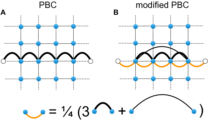
Figure S4: Periodic boundary conditions (PBC) vs. modified periodic boundary conditions (mPBC). Here we exemplify how a specific form of couplings – those connecting nearest neighbors – change when going from PBC to mPBC. (A) The black arcs indicate nearest-neighbor couplings for PBC. On a torus, these couplings connect boundary sites to the periodic image of the sites on the opposite boundary (indicated with the open circles); (B) the orange arcs indicate the same couplings for mPBC, and are given by the average between the nearest-neighbor couplings and the dipolar coupling between opposite sites, which are nearest neighbors on the torus (see the formula indicated in the figure).

When using periodic boundary conditions, the couplings $J_{ij}$ are calculated by taking distances between sites on a torus, with a maximal distance of $L/2$ for a $L\times L$ square lattice: in the case of dipolar interactions $J^{\rm(FM)}_{ij,\rm PBC}=J/(r^{(t)}_{ij})^{3}$, with a distance on the torus $r^{(t)}_{ij}=[\min^{2}(|x_{i}-x_{j}|,L-|x_{i}-x_{j}|)+\min^{2}(|y_{i}-y_{j}|,L-|y_{i}-y_{j}|)]^{1/2}$ (see Fig. S4A), and as before $J_{ij,\rm PBC}^{\rm(AFM)}=(-1)^{i+j+1}J_{ij,\rm PBC}^{\rm(FM)}$.

To perform the Bogolyubov diagonalization of the quadratic bosonic Hamiltonian on a periodic lattice, we consider the Fourier transformed Bose operators, $b_{\bm{k}}=\sum_{i}e^{-i\bm{k}\cdot\bm{r}_{i}}b_{i}/\sqrt{N}$. Introducing the operators $a_{\bm{k}}$ and $a^{\dagger}_{\bm{k}}$ such that $a_{\bm{k}}=u_{\bm{k}}b_{\bm{k}}+v_{\bm{k}}b^{\dagger}_{-\bm{k}}$ leads to the diagonal form $H_{2}=\sum_{\bm{k}}\hbar\omega_{\bm{k}}a_{\bm{k}}^{\dagger}a_{\bm{k}}+\sum_{\bm{k}}(\epsilon_{\bm{k}}-A_{\bm{k}})/2$ where $A_{\bm{k}}=J(\gamma^{(t)}_{0}-\gamma^{(t)}_{\bm{k}}/2)$, and $\omega_{\bm{k}}$ is given in the main text. Here (and contrarily to the main text) $\gamma^{(t)}_{\bm{k}}$ is the Fourier transform of the dipolar interactions defined on a torus, $\gamma^{(t)}_{\bm{k}}=N^{-1}\sum_{i\neq j}\eta^{i+j+1}/(r^{(t)}_{ij})^{3}$ with $\eta=1(-1)$ for the FM (AFM). The bosonic quasiparticles associated with the Bogolyubov operators $a_{\bm{q}},a_{\bm{q}}^{\dagger}$ are called magnons, and they represent the linearized excitations of the system.

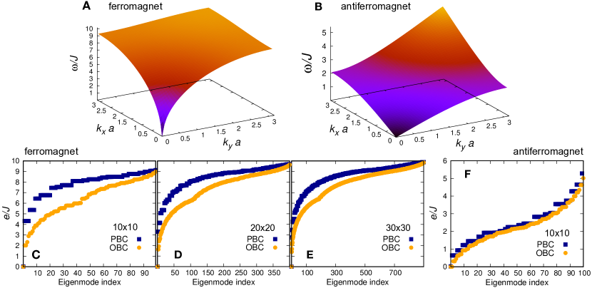
Figure S5: Dispersion relation of the dipolar 2d XY model from linear spin-wave theory. (A): ferromagnet; (B): antiferromagnet. (C-E): Eigenenergies from linear spin-wave theory for the 2d XY dipolar ferromagnet. We contrast periodic (PBC) with open (OBC) boundary conditions, for three system sizes: (C): $10\times 10$; (D): $20\times 20$; (E): $30\times 30$. (F): Eigenenergies from linear spin-wave theory for the 2d XY dipolar antiferromagnet, contrasting periodic (PBC) with open (OBC) boundary conditions on a $10\times 10$ lattice.

The dispersion relations of the dipolar ferromagnet and antiferromagnet are shown in Fig. S5A,B. They exhibit the characteristic nonlinear behavior $\omega_{\bm{k}}\sim\sqrt{k}$ at small $k$ for the ferromagnet, as well as linear behavior $\omega_{\bm{k}}\sim k$ for the antiferromagnet.

The time-dependent structure factor has a simple form within linear spin-wave theory [10]:

$$S({\bm{k}},t) = \langle b^{\dagger}_{\bm{k}}b^{\dagger}_{\bm{k}}+b_{-\bm{k}}b^{\dagger}_{-\bm{k}}-b_{\bm{k}}b_{-\bm{k}}-b^{\dagger}_{\bm{k}}b^{\dagger}_{-\bm{k}}\rangle$$ (11)

$$= C_{\bm{k}}+D_{\bm{k}}\cos(2\omega_{\bm{k}}t)\ ,$$

where $C_{\bm{k}}=1-\gamma^{(t)}_{\bm{k}}/(2\gamma^{(t)}_{0})$ and $D_{\bm{k}}=\gamma^{(t)}_{\bm{k}}/(2\gamma^{(t)}_{0})$. It features a term at zero frequency (corresponding to the constant term) as well as a term at frequency $2\omega_{\bm{k}}$, as expected from the discussion of quench spectroscopy in Sec. III. Moreover, LSW theory yields a relation between the constant $C_{\bm{k}}$ and the frequency $\omega_{\bm{k}}=J\gamma^{(t)}_{0}\sqrt{2C_{\bm{k}}-1}\leavevmode\nobreak\$.

IV.2 Open boundary conditions

For lattices with open boundary conditions, one can still diagonalize the Hamiltonian of Eq. (10) via a generalized Bogolyubov transformation $a_{\alpha}=\sum_{i}(u_{i}^{(\alpha)}b_{i}+v_{i}^{(\alpha)}b_{i}^{\dagger})$ which brings the quadratic Hamiltonian to the form $H_{2}=\sum_{\alpha}\hbar\omega_{\alpha}a_{\alpha}^{\dagger}a_{\alpha}+{\rm const}$. To do so, one builds the $N\times N$ matrices $A$ and $B$, with $2A_{ij}=\left(\sum_{k}J_{ik}\leavevmode\nobreak\ \delta_{ij}-J_{ij}/2\right)$ and $B_{ij}=J_{ij}/4$. One then diagonalizes the $2N\times 2N$ non-Hermitian matrix $\begin{pmatrix}A&B\\ -B&-A\end{pmatrix}$ with a matrix of right eigenvectors $\begin{pmatrix}U&-V\\ -V&U\end{pmatrix}$ where $U_{i\alpha}=u_{i}^{(\alpha)}$ and $V_{i\alpha}=v_{i}^{(\alpha)}$ are $N\times N$ matrices [35, 36], assumed here to be real-valued (as is the case for the models studied in this work).

IV.3 Effect of boundary conditions on the linear spin-wave eigenspectrum

The experiments of this work are performed on lattices with open boundary conditions (OBC). It is thus important to compare the linear spin-wave spectrum on open lattices with that of lattices with periodic boundary conditions (PBC). Figures. S5C,F show the ordered eigenfrequencies spectrum $\omega_{\alpha}$ for square lattices with PBC and OBC for both the XY dipolar ferromagnet and the antiferromagnet. The eigenfrequencies of the ferromagnet with OBC are systematically smaller than those of the same model with PBC: this is a consequence of the dipolar interactions, which enhance the role of boundary conditions with respect to e.g. nearest-neighbor interactions. In particular the discrepancy between the OBC and PBC spectra persists for large lattices, and it is still visible when tripling the linear size of the lattice (from $10\times 10$ to $30\times 30$). Contrarily, the antiferromagnet is less sensitive to boundary conditions, and already on the $10\times 10$ lattice the OBC and PBC spectra are very close. This is a manifestation of the effectively short-ranged nature of the antiferromagnetic interactions, due to frustration: sites close to the boundary of an OBC system and sites in the bulk experience almost the same interactions, and boundary effects are less important.

The results in Fig. S5C,E may suggest that quench spectroscopy experiments on the ferromagnet on e.g. a $10\times 10$ lattice will reconstruct a very different dispersion relation than the one predicted for the PBC system. Moreover, this reconstruction will be complicated by the fact that the eigenmodes of the ferromagnet do not correspond to plane waves, and therefore the momentum-dependent spin-flip operators $\sigma_{\pm\bm{k}}^{z}$ excite a superposition of them. This difficulty is in fact overcome when considering the system dynamics at sufficiently short times, thanks to a short-time projective equivalence between the OBC system and a system with modified PBC as we explain in the next section.

V Projective equivalence between OBC and modified-PBC lattices at short times

V.1 Momentum-sector decomposition of the Hilbert space and of the Hamiltonian

As already pointed out above, a PBC lattice has the topology of a torus, and its properties are invariant under translations $T_{\bm{d}}$ by a vector $\bm{d}=(d_{x},d_{y})$ along the torus. The eigenvectors of the Hamiltonian with PBC are therefore also eigenvectors of the symmetry operator $T_{\bm{d}}$, namely states $|\Psi_{\bm{Q}}\rangle$ with definite total momentum ${\bm{Q}}$, such that $T_{\bm{d}}|\Psi_{\bm{Q}}\rangle=e^{i\bm{Q}\cdot\bm{d}}|\Psi_{\bm{Q}}\rangle$.

An OBC lattice can also be thought of as being wrapped to form a torus. However, the couplings $J_{ij}$ depend on the standard euclidean distance between sites (and not on the distance on the torus), $J_{ij}=J/r^{3}_{ij}$ with $r_{ij}=[(x_{i}-x_{j})^{2}+(y_{i}-y_{j})^{2}]^{1/2}$. As a consequence the system with OBC is not invariant under translations $T_{\bm{d}}$ on the torus.

Yet, even for the OBC lattice, it is useful to keep a picture of Hilbert space as being structured into different momentum sectors, with related projectors ${\cal P}_{\bm{Q}}=\sum_{\Psi_{\bm{Q}}}|\Psi_{\bm{Q}}\rangle\langle\Psi_{\bm{Q}}|$, such that $\sum_{\bm{Q}}{\cal P}_{\bm{Q}}=\mathds{1}$. The Hamiltonian $H_{\rm OBC}$ on a OBC lattice, when written on the basis of momentum eigenstates, will then possess a diagonal part as well as an off-diagonal one $H_{\rm OBC}=H_{\rm D}+H_{\rm OD}$ with

$$H_{\rm D}=\sum_{\bm{Q}}{\cal P}_{\bm{Q}}H_{\rm OBC}{\cal P}_{\bm{Q}}\ ,\ H_{\rm OD}=\sum_{\bm{Q}\neq\bm{Q}^{\prime}}{\cal P}_{\bm{Q}}H_{\rm OBC}{\cal P}_{\bm{Q}^{\prime}}.$$ (12)

In the case of the Hamiltonian Eq. (9), the diagonal and off-diagonal parts are readily identifiable as

$$H_{\rm D} = \frac{J}{2}\sum_{\bm{k}}{\gamma}_{\bm{k}}\left(\sigma_{\bm{k}}^{x}\sigma_{-\bm{k}}^{x}+\sigma_{\bm{k}}^{y}\sigma_{-\bm{k}}^{y}\right)$$

$$H_{\rm OD} = \frac{J}{2}\sum_{\bm{k}\neq\bm{k}^{\prime}}\Gamma_{\bm{k},\bm{k}^{\prime}}\left(\sigma_{\bm{k}}^{x}\sigma_{-\bm{k}^{\prime}}^{x}+\sigma_{\bm{k}}^{y}\sigma_{-\bm{k}^{\prime}}^{y}\right)$$ (13)

where

$$J\Gamma_{\bm{k},\bm{k}^{\prime}}=\frac{1}{N}\sum_{ij}e^{i({\bm{k}}\cdot\bm{r}_{i}-{\bm{k}^{\prime}}\cdot\bm{r}_{j})}\leavevmode\nobreak\ J_{ij}$$ (14)

and $\gamma_{\bm{k}}=\Gamma_{\bm{k},\bm{k}}$ – coinciding with the one used in the main text. The diagonal part $H_{D}$ is an effective Hamiltonian with periodic boundary conditions, and modified couplings $\tilde{J}_{ij,\rm mPBC}=\tilde{J}({\bm{r}^{(t)}_{ij}})$ where ${\bm{r}}^{(t)}_{ij}$ is a distance on the torus, and

$$\tilde{J}({\bm{r}})=\frac{J}{N}\sum_{\bm{k}}e^{-i\bm{k}\cdot\bm{r}}\gamma_{\bm{k}}=\frac{1}{N}\sum_{hl}J_{hl,\rm OBC}\leavevmode\nobreak\ \delta_{{\bm{r}}^{(t)}_{hl},\bm{r}}\ .$$ (15)

Thus, $\tilde{J}({\bm{r}})$ is the average coupling between all sites on the OBC lattice that possess that same distance ${\bm{r}}^{(t)}_{hl}={\bm{r}}$ on the torus. In the following we denote the Hamiltonian $H_{\rm D}$ as the Hamiltonian with modified PBC (mPBC).

All the results of spin-wave theory for PBCs, described in Sec. IV.1, apply as well to the Hamiltonian with mPBC after the simple substitution $\gamma^{(t)}_{\bm{k}}\to\gamma_{\bm{k}}$.

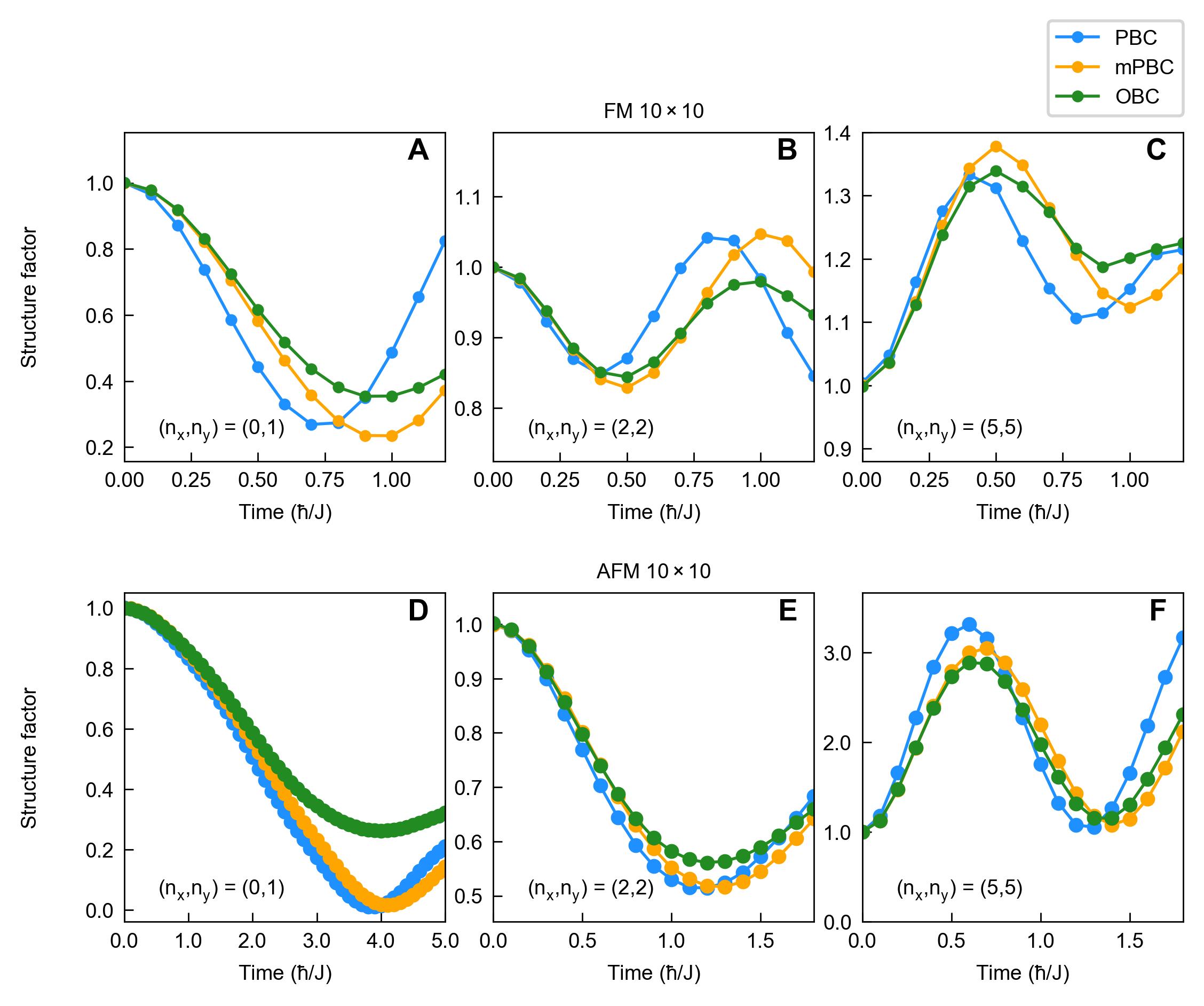
Figure S6: Time-dependent structure factor at short times for different boundary conditions, obtained by tVMC on a $10\times 10$ lattice. Comparison between periodic (PBC), modified-periodic (mBPC) and open (OBC) boundary conditions for three wavevectors ${\bm{k}}a/\pi=(0,1)$, $(2,2)$ and $(5,5)$ for the ferromagnet (panels (A), (B) and (C)) and the antiferromagnet (panels (D), (E) and (F)).

V.2 Short-time projective equivalence with uniform initial states

The momentum structure of the OBC Hamiltonian (13) is relevant when considering unitary evolutions that start in a definite momentum sector. This is the case of the homogeneous initial states considered in this study, namely the CSS state, which is a momentum eigenstate with ${\bm{Q}}=0$.

As a consequence, inserting the completeness relation on the momentum basis $\sum_{\bm{Q}}{\cal P}_{\bm{Q}}=\mathds{1}$ in Eq.(5), the time-dependent structure factor of the OBC system can be rewritten as

$$S(\bm{k},t)=S_{\rm mPBC}(\bm{k},t)+\Delta S(\bm{k},t)$$ (16)

where

$$S_{\rm mPBC}(\bm{k},t)=\langle{\rm CSS}|e^{iH_{\rm D}t/\hbar}\sigma_{\bm{k}}^{z}\sigma_{-\bm{k}}^{z}e^{-iH_{\rm D}t/\hbar}|{\rm CSS}\rangle$$ (17)

is related to the dynamics governed by $H_{\rm D}$, restricted to the zero-momentum sector in which it is initialized. The term

$$\Delta S(\bm{k},t)$$

$$=\sum_{\bm{Q}\neq 0}\langle{\rm CSS}|{\cal P}_{0}e^{iH_{\rm OD}t/\hbar}{\cal P}_{\bm{Q}}\sigma_{\bm{k}}^{z}\sigma_{-\bm{k}}^{z}{\cal P}_{\bm{Q}}e^{-iH_{\rm OD}t/\hbar}{\cal P}_{0}|{\rm CSS}\rangle$$ (18)

is the contribution related to the leaking of the dynamics into non-zero momentum sectors under the effect of $H_{\rm OD}$.

At the beginning of the dynamics $S(\bm{k},0)=S_{\rm mPBC}(\bm{k},0)$ and $\Delta S(\bm{k},0)=0$ by virtue of the choice of the initial state. Therefore there must be an interval $[0,t_{\rm PE}]$ in the early evolution during which

$$t\in[0,t_{\rm PE}]:S(\bm{k},t)\approx S_{\rm PBC}(\bm{k},t)\ .$$ (19)

Thus, over this early evolution time, the dynamics of the time-dependent structure factor is (nearly) projectively equivalent to that of a system with the same lattice structure but with PBC, and possessing the modified couplings of Eq. (15). The duration $t_{\rm{PE}}$ of the approximate projective equivalence (OBC $\approx$ modified PBC) is difficult to estimate a priori, but it certainly extends to longer times the larger the system size, as for $N\to\infty$ the three lattice geometries – OBC, PBC and modified PBC – will eventually give the same physics.

We have numerically tested the effective duration of the projective equivalence by comparing the dynamics of the time-dependent structure factor in the OBC system with that of modified-PBC system. Figure S6 shows the tVMC predictions for the time-dependent structure factor of a $10\times 10$ lattice with PBC, OBC and mPBC, both for the case of the dipolar FM and AFM, and for three representative wavevectors going from the center to the edge of the Brillouin zone. We observe a nearly exact projective equivalence between OBC and mPBC dynamics at short times, and an approximate projective equivalence persists at times of the order of an interaction cycle $J^{-1}$ – enough to observe a first complete oscillation of the time-dependent structure factor. Over this oscillation the modification of the couplings in the PBC system is what it takes to quantitatively account for the shift of the oscillation frequency when going from (standard) PBC to OBC.

We therefore conclude that, when the initial state is an eigenstate of the lattice momentum, the short-time dynamics of the time-dependent structure factor of an OBC lattice allows for the reconstruction of the excitation spectrum of an effective system with PBC – namely a spectrum which admits the wavevector ${\bm{k}}$ as a meaningful label of the eigenfrequencies, and therefore which defines a dispersion relation in the proper sense.

VI Density of excitations triggered by the quench, and relationship to the thermodynamics

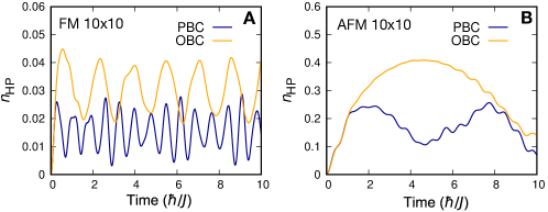
Figure S7: Density of finite-momentum Holstein-Primakoff (HP) bosons generated by the dynamics. (A): time-dependent density of finite-momentum (FM) HP bosons generated along the linear spin-wave theory dynamics of the FM on a $10\times 10$ lattice with PBC and OBC; (B): same result for the AFM.

The amount of excitations triggered by the initial quench can be estimated via linear spin-wave theory in two alternative ways. In the case of periodic boundary conditions, one can simply calculate the density of finite-momentum magnons which are present in the initial state, $n_{m}=\frac{1}{N}\sum_{\bm{k}\neq 0}\langle a_{\bm{k}}^{\dagger}a_{\bm{k}}\rangle=\frac{1}{N}\sum_{\bm{k}\neq 0}v_{\bm{k}}^{2}$. For a $10\times 10$ lattice we find that $n_{m}\approx 7.4\times 10^{-3}$ for the FM and $n_{m}\approx 6.6\times 10^{-2}$ for the AFM. The two densities differ by an order of magnitude, exhibiting the enhanced role of fluctuations in the case of the AFM compared with the FM. The small values of the densities may suggest that neglecting non-linear bosonic terms in the Hamiltonian, leading to spin-wave theory, is well justified in both cases.

Nonetheless the above observation needs to be reconsidered when calculating instead the density of finite-momentum HP bosons generated during the quench dynamics. This density is defined as $n_{\rm HP}=\frac{1}{N}\sum_{\bm{k}\neq 0}\langle b_{\bm{k}}^{\dagger}b_{\bm{k}}\rangle$; the approximation leading to Eq. (10) can be considered to be valid if $n_{\rm HP}$ remains much smaller than its maximum value, $2s=1$, at least for finite-momentum bosons. The zero-momentum ones, corresponding to the zero mode of the U(1) symmetric Hamiltonian, can be treated separately as a non-linear rotor variable: They do not contribute to the correlations in the $S^{z}$ spin components [37]. On the contrary, a large density of finite-momentum HP bosons implies that the linearization of the Hamiltonian dynamics is a poor approximation: boson-boson interactions must be accounted for, as well as the coupling between the zero-momentum bosons and the finite-momentum ones.

The time evolution of $n_{\rm HP}$ is shown in Figure S7. We observe that the FM dynamics develops a density of finite momentum bosons reaching peak values of $n_{\rm FM}\approx 0.04$ (with OBC). Contrarily, the largest value for the AFM is an order of magnitude higher, bringing the system to a regime in which the population of HP bosons can no longer be considered as dilute. This shows that non-linearities are expected to play a very different role for the AFM with respect to the FM.

VII Numerical methods

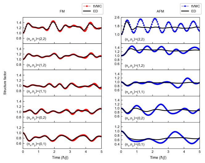
Figure S8: Comparison between tVMC and exact diagonalization for the time-dependent structure factor of the dipolar XY model on a $4\times 4$ lattice (with OBC) for all the non-equivalent wavevectors in the Brillouin zone. Left panels: ferromagnet; right panels: antiferromagnet.

The theoretical results for the time evolution of dipolar spin Hamiltonians have been obtained using time-dependent linear spin-wave theory (discussed in Sec. IV), and two numerical approches: 1) exact diagonalization on small ($4\times 4$) lattices (using the QuSpin package [38]); and 2) time-dependent variational Monte Carlo (tVMC). The latter approach is based on the time evolution of a trial wavefunction governed by the time-dependent variational principle [39]. We used a spin-Jastrow (or pair-product) wavefunction [40, 41] for the present study, as this wavefunction has already proven to be very successful in reproducing the non-equilibrium physics of the dipolar XY ferromagnet [41, 18] (tested by comparison with exact diagonalization on small systems): Figure S8A shows the tVMC predictions for $S(\bm{k},t)$ of the FM with OBC together with exact diagonalization ($4\times 4$ lattice), confirming its ability to grasp the correct behavior over the entire time scale relevant for the experiment. As a consequence, we use tVMC to extend the numerical predictions beyond exact diagonalization, and up to the $10\times 10$ OBC lattices implemented in the experiment.

In the case of the dipolar antiferromagnet, though, the ability of the Jastrow wavefuction to reproduce the correct non-equilibrium evolution is much more limited. When comparing with exact diagonalization (see Fig. S8B), tVMC based on Jastrow wavefunction reproduces correctly the early-time dynamics – most importantly for us, the first oscillations of the time-dependent structure factor – until a time of order $\hbar/J$. However, the Jastrow wavefunction misses the later decay of the oscillations. Hence we can use the tVMC results to extract characteristic wavevector-dependent frequencies in the early-time dynamics, independently of spin-wave theory.

In the case of the ferromagnet, we can also make quantitative predictions for the thermal state towards which the dynamics is expected to relax at long times. This state should be dictated uniquely by the conserved quantities in the dynamics: If the energy is the only conserved quantity, the thermal state is given by the Gibbs ensemble (GE) at the temperature $T_{\rm CSS}$ such that $\langle{\rm CSS}|H|{\rm CSS}\rangle=\langle H\rangle_{T_{\rm CSS}}$, where $\langle...\rangle_{T}={\rm Tr}[e^{-H/(k_{B}T)}(...)]/{\rm Tr}[e^{-H/(k_{B}T)}]$ is the GE average at temperature $T$. The dynamics of the dipolar XY model also conserves the collective spin $J^{z}=\sum_{i}\sigma_{i}^{z}$ and all its functions. Of particular interest for us is $\langle{\rm CSS}|(J^{z})^{2}|{\rm CSS}\rangle=N$, which corresponds to the structure factor at zero wavevector $S(0)=\langle(J^{z})^{2}\rangle/N$. Hence, in order to correctly capture the structure factor of the equilibrium state to which the dynamics should relax, we run quantum Monte Carlo (QMC) simulations (based on the stochastic series expansion approach [42]) in the generalized Gibbs ensemble (GGE), in which averages are calculated as $\langle...\rangle_{T,\lambda}={\rm Tr}\{e^{-[H/(k_{B}T)-\lambda(J^{z})^{2}]}(...)\}/{\rm Tr}\{e^{-[H/(k_{B}T)-\lambda(J^{z})^{2}]}\}$, where $\lambda$ is a Lagrange multiplier tuned so that $\langle(J^{z})^{2}\rangle_{T,\lambda}=N$. Our GGE QMC simulations are performed on a $N=100$ array with open boundary conditions, in order to mimic closely the experiment. For this lattice size, the temperature matching the initial-state energy is $T/J\approx 1.2$.

Some finite-temperature calculations are possible for the dipolar antiferromagnet using tensor network methods, albeit at restricted system sizes. Following the methodology described in Ref. [17], we use minimally entangled typical thermal states to estimate an energy-temperature calibration. For a $4\sqrt{2}\times 8\sqrt{2}=64$ site cylinder, we find $T_{\mathrm{CSS}}^{\mathrm{AFM}}/J\approx 0.6$. As a benchmark, carrying out the same procedure for the nearest-neighbor model gives a value of $T_{\mathrm{CSS}}^{\mathrm{nearest-neighbor}}$ differing by about 10$\%$ from prior QMC results [43]. We attribute this discrepancy to strong finite-size effects near the Berezinskii-Kosterlitz-Thouless transition – namely, our system size is comparable to the correlation length $\xi/a\approx 23$ found at $T_{\mathrm{CSS}}^{\mathrm{nearest-neighbor}}$ [43].

VIII Ground-state spectral functions vs. quench spectroscopy for dipolar XY models

We discuss here the spectral function accessible to quench spectroscopy, and compare it with more conventional spectral functions (i.e. the dynamical structure factor and its generalizations), obtained by probing the linear response of the system at thermal equilibrium. In particular, using exact diagonalization to calculate the conventional spectral functions, we gather informations on the nature of the spectrum of elementary excitations in the dipolar XY models.

VIII.1 Quench spectral function vs. dynamical structure factors

The Fourier transform of the time-dependent structure factor given by Eq. (7), monitored over an infinite time, reconstructs the quench spectral function:

$${\cal Q}(\bm{k},\omega)=\sum_{nm}\langle\Psi(0)|n\rangle\langle m|\Psi(0)\rangle\langle n|\sigma_{\bm{k}}^{z}\sigma_{-\bm{k}}^{z}|m\rangle\delta(\omega-\omega_{nm})\leavevmode\nobreak\ .$$ (20)

As discussed in Sec. III, this spectral function contains contributions from all the transitions $|m\rangle\to|n\rangle$ among states which are connected by two spin flips at opposite momenta and which have a significant overlap with the initial state of the quench dynamics.

Contrarily, the conventional spectral function associated with $\sigma^{z}_{\bm{k}}$ operator, and relevant for spectroscopy at thermal equilibrium, is the one-spin-flip dynamical structure factor:

$${\cal S}_{1}(\bm{k},\omega)=\frac{1}{\cal Z}\sum_{nm}e^{-\beta E_{m}}|\langle n|\sigma_{\bm{k}}^{z}|m\rangle|^{2}\delta(\omega-\omega_{nm})$$ (21)

where $\beta=(k_{B}T)^{-1}$ is the inverse temperature. This structure factor is probed e.g. by neutron scattering, as it dictates the scattering cross sections of neutrons from magnetic materials at thermal equilibrium [7]. At variance with the quench spectral function ${\cal Q}(\bm{k},\omega)$, ${\cal S}_{1}(\bm{k},\omega)$ probes transitions among states connected by a single spin-flip operator $\sigma^{z}_{\bm{k}}$. Here, the final state of the transitions needs not be thermally populated.

It is then instructive to consider a two-spin-flip dynamical structure factor, defined as

$${\cal S}_{2}(\bm{k},\omega)=\frac{1}{\cal Z}\sum_{nm}e^{-\beta E_{m}}|\langle n|\sigma_{\bm{k}}^{z}\sigma_{-\bm{k}}^{z}|m\rangle|^{2}\delta(\omega-\omega_{nm})$$ (22)

which probes instead the same transitions as those that contribute to the quench spectral function, although not with the same weights. Related spectral functions are measured in condensed-matter experiments by two-magnon Raman scattering [44] and resonant inelastix X-ray scattering [45].

In the following we contrast these three spectral functions in the case of the dipolar XY models.

VIII.2 Spectral functions for dipolar XY magnets from exact diagonalization

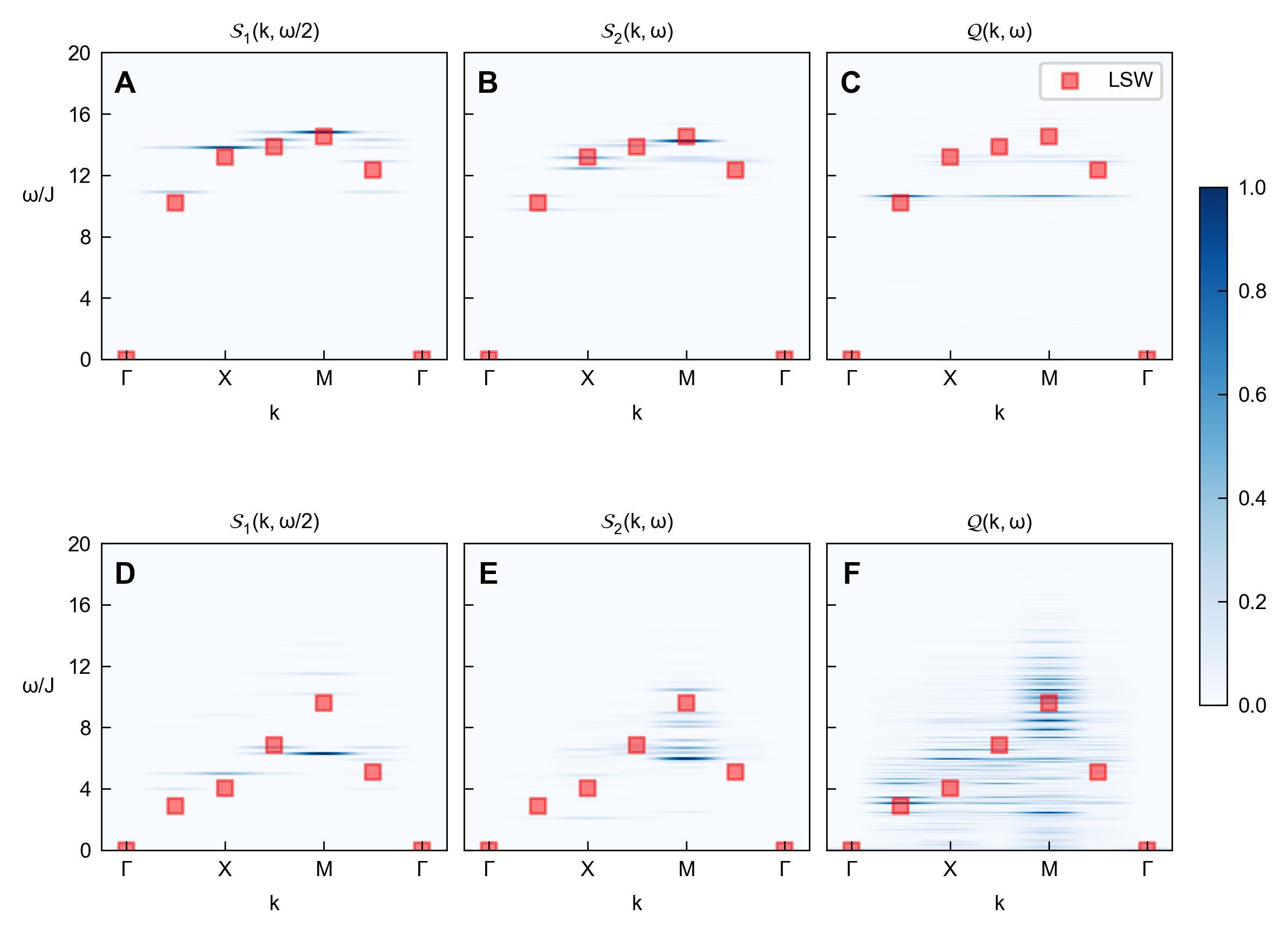
Figure S9: Spectral functions for the $4\times 4$ dipolar XY model (with PBC). (A),(D): Zero-temperature one-spin-flip dynamical structure factor ${\cal S}_{1}(\bm{k},\omega)$ for the ferromagnet (A) and the antiferromagnet (D); (B),(E) zero-temperature two-spin-flip dynamical structure factor ${\cal S}_{2}(\bm{k},\omega)$ for the ferromagnet (B) and the antiferromagnet (E); (C),(F) Quench spectral function (referred to the coherent spin state) ${\cal Q}(\bm{k},\omega)$ for the ferromagnet (C) and the antiferromagnet (F). The ${\bm{k}}$ vectors are taken along the the path indicated in Fig. 4 of the main text. The red squares mark the dispersion relation from linear spin-wave theory. In all the panels, the values of the spectral functions are normalized to their maximum.

Figure S9 shows the one- and two-spin-flip dynamical structure factors at $T=0$, as well as the quench spectral function, for both the ferromagnetic and antiferromagnetic dipolar XY models on a $4\times 4$ lattice with PBC, obtained via exact diagonalization. The $T=0$ dynamical structure factors reveal the spectrum of excitations created by the spin-flip operators $\sigma_{\bm{k}}^{z}$ and $\sigma_{\bm{k}}^{z}\sigma_{-\bm{k}}^{z}$ onto the Hamiltonian ground state.

Figures S9A,B show that, for the dipolar ferromagnet, the spectrum of two-spin-flip excitations corresponds to twice the spectrum for the single-spin-flip ones – highlighting the free quasiparticle nature of the excitations themselves. This is further confirmed by the correspondence between the characteristic frequencies of the one-spin-flip and two-spin-flip spectra compared to the predictions of linear spin-wave theory. The quench spectral function (Fig. S9C) has also a similar structure to that of the two-spin-flip dynamical structure factor, but with additional lower frequencies: These correspond to transitions which do not involve the Hamiltonian ground state.

A different picture emerges for the dipolar antiferromagnet, as shown in Figs. S9D,F. The one-spin-flip structure factor (Fig. S9D) exhibits multiple frequencies for the same wavevector with similar spectral weight. For the wavevector $(\pi,\pi)$ ($M$-point) a dominant frequency emerges, which nonetheless differs significantly from the spin-wave prediction. As we discuss in Sec. IX, the first nonlinear correction to spin-wave theory leads to a finite decay rate of single-magnon excitations at $(\pi,\pi)$, which may indeed be reflected in the result on the small size accessible to exact diagonalization. This already suggests a significant departure of the elementary excitation spectrum from that of free quasiparticles. Yet the most dramatic departure is seen at the level of the two-spin-flip structure factor (Fig. S9E), which shows an even broader spectrum of frequencies at essentially all wavevectors, and especially so at $(\pi,\pi)$, where a “continuum” of frequencies emerges. This result suggests that two-magnon-decay processes may be even more prominent that single-magnon ones. The broad spectral features observed in the two-spin-flip structure factor are much more prominently revealed in the quench spectral function (Fig. S9F), whose structure is consistent with the fast decay of oscillations of the time-dependent structure factor revealed by the experiment, as discussed in the main text.

IX One-magnon decay

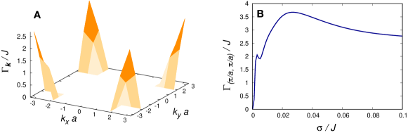
Figure S10: Single-magnon decay rate. (A) $\Gamma_{\bm{k}}$ for the spin-wave modes of a $10\times 10$ dipolar XY antiferromagnet. The Dirac function entering in Eq. (24) has been broadened to a Gaussian with width $\sigma=0.01J$. (B) $\sigma$-dependence of the decay rate for the spin-wave mode at ${\bm{k}}=(\pi/a,\pi/a)$.

To test the robustness of spin-wave predictions beyond the harmonic approximation we consider the first nonlinear correction to the quadratic Hamiltonian Eq. (10), and calculate its effect on possible decay of single-magnon excitations using Fermi’s golden rule [46]. The first nonlinear correction to the quadratic Hamiltonian is the quartic Hamiltonian, expressed in momentum space:

$$H_{4}=\frac{1}{N}\sum_{\bm{k}\bm{k}^{\prime}\bm{q}}\Big{[} {\cal A}_{\bm{k}\bm{k}^{\prime}\bm{q}} b_{\bm{k}-\bm{q}}^{\dagger}b_{\bm{k}^{\prime}+\bm{q}}^{\dagger}b_{\bm{k}}b_{\bm{k}^{\prime}}$$

$$+ {\cal B}_{\bm{k}\bm{k}^{\prime}\bm{q}} \Big{(}b_{\bm{k}}^{\dagger}b_{\bm{k}^{\prime}}^{\dagger}b_{\bm{q}-\bm{k}-\bm{k}^{\prime}}^{\dagger}b_{\bm{q}}+{\rm h.c.}\Big{)}\leavevmode\nobreak\ \Big{]}$$ (23)

where ${\cal A}_{\bm{k}\bm{k}^{\prime}\bm{q}}=J_{\bm{q}}-(J_{\bm{k}^{\prime}}+J_{\bm{k}-\bm{q}})/4$ and ${\cal B}_{\bm{k}\bm{k}^{\prime}\bm{q}}=-(J_{\bm{k}}+J_{\bm{q}-\bm{k}-\bm{k}^{\prime}})/8$. It can be Bogolyubov transformed to a quartic Hamiltonian in terms of the magnon operators $a_{\bm{k}},a_{\bm{k}}^{\dagger}$. The resulting expression is rather lengthy but straightforward to obtain. In a system with periodic boundary conditions, this Hamiltonian leads to a decay process of a single magnon into three magnons via terms of the form $a^{\dagger}_{{\bm{q}}_{1}}a^{\dagger}_{{\bm{q}}_{2}}a^{\dagger}_{{\bm{q}}_{3}}a_{\bm{k}}$, conserving momentum (${\bm{k}}={\bm{q}}_{1}+{\bm{q}}_{2}+{\bm{q}}_{3}$) and energy ($\omega_{\bm{k}}=\omega_{1}+\omega_{2}+\omega_{3}$), with a rate [46]:

$$\Gamma_{\bm{k}}=\frac{\pi}{8\hbar}\sum_{\bm{q}_{1},\bm{q}_{2}}\langle 1_{\bm{q}_{1}},1_{\bm{q}_{2}},1_{\bm{k}-\bm{q}_{1}-\bm{q}_{2}}|H_{4}|1_{\bm{k}}\rangle|^{2}$$ (24)

$$\delta(\omega_{\bm{k}}-\omega_{1}-\omega_{2}-\omega_{3})$$

where the states $|\{n_{\bm{q}}\}\rangle$ are Fock states of magnon occupation. To calculate the decay rate on a finite-size system, the $\delta$ function of Eq. (24) is given a finite width, e.g. by approximating it with a Gaussian $\delta(x)\to\exp[-x^{2}/(2\sigma^{2})]/(\sqrt{2\pi}\sigma)$. The finite (i.e. non-zero) width corresponds to a finite (i.e. not infinite) observation time, in which energy needs not be perfectly conserved. The numerical value of $\Gamma_{\bm{k}}$ depends on $\sigma$, but only weakly when $\sigma$ is sufficiently large (e.g. $\sigma/J\gtrsim 5\times 10^{-3}$ for a $10\times 10$ system, as shown in Fig. S10B).

In the case of the dipolar ferromagnet, the calculation of the decay rate leads to a negligible result – consistent with the robustness of linear spin-wave theory. Contrarily, in the antiferromagnet case, a significant decay rate emerges for ${\bm{k}}\approx(\pi,\pi)$, as shown in Fig. S10A. The propensity to decay of antiferromagnetic magnons can be understood by inspecting the dispersion relation of Fig. S5: such a dispersion relation is nearly linear close to the diagonal of the Brillouin zone connecting the origin to the $(\pi,\pi)$ corner. This allows for the decay channels ${\bm{k}}\to{\bm{q}}_{1}+{\bm{q}}_{2}+{\bm{q}}_{3}$ which conserve energy, and which are more numerous the closer ${\bm{k}}$ is to $(\pi,\pi)$.

The latter result suggests that the decay of oscillations in the time-dependent structure factor observed in the experiment can be – at least partially – traced back to the decay process of single-magnon excitations. Nonetheless the initial state of the experiment – the coherent spin state along $y$ – corresponds to a finite density of magnons, so that multi-magnon decay processes are expected to be as relevant as single-magnon ones. In fact, the two-spin-flip dynamical structure factor shown in Sec. VIII.2 shows a richer frequency content than the single-spin-flip one, which suggests already the importance of two-magnon decay processes compared to single-magnon ones. A full study of the (multi-)magnon decay processes quantitatively explaining the damping of oscillations observed in the experiment goes far beyond the scope of the present work. Yet this aspect deserves further investigations, in order to understand more deeply the insight into the nature of elementary excitations which is provided by quench spectroscopy.