The delay feedback control for the McKean-Vlasov stochastic differential equations with common noise

Abstract

Motivated by the stabilization problem of McKean-Vlasov stochastic differential equations (SDEs) with common noise by the delay feedback control, this paper studies a class of McKean-Vlasov stochastic functional differential equations (SFDEs) with common noise in which the dynamic of the underlying process depends on its history. This paper first investigates the well-posedness of McKean-Vlasov SFDEs with common noise under the global Lipschitz condition by the fixed point theorem and derives the conditional propagation of chaos. Secondly, the paper studies the stability theory of a class of McKean-Vlasov SFDEs with common noise and the stability equality between the McKean-Vlasov SFDEs with common noise and the corresponding particle system. Thirdly, by using this theory, this paper analyzes the stabilization of the McKean-Vlasov SDEs with common noise by the delay feedback control and gives the delay bound.

Keywords. McKean-Vlasov SDEs, Common noise, Particle system, Stabilization, Delay feedback control.

1 Introduction

The McKean-Vlasov stochastic differential equations (SDEs) with common noise, viewed as the limit equation of a single particle in the mean-field particle system subject to a common noise as the number of particles goes to infinity, have been widely applied in finance, physics, biology, mean-field games, machine learning, and so on [2, 6, 7, 10, 12, 13, 16, 17, 20, 22, 23, 24, 31, 32, 36]. It is worth noting that solutions to the McKean-Vlasov SDEs with common noise correspond to the measure valued solution of a nonlinear stochastic partial equations [18]. One classical form of this kind of SDEs reads as follows:

$$\begin{aligned} \mathrm{d}X(t)&=f\left(t,X(t),\mathcal{L}^{1}(X(t))\right)\mathrm{d}t+g\left(t,X(t),\mathcal{L}^{1}(X(t))\right)\mathrm{d}B_{t}\\ &\quad+g^{0}\left(t,X(t),\mathcal{L}^{1}(X(t))\right)\mathrm{d}B_{t}^{0},\end{aligned}$$ (1.1)

where $(\mathcal{L}^{1}(X(t)))_{t\geq 0}$ denotes the conditional distributions of $X$ given the common source of noise $B^{0}$ (see section 2 for the rigorous probabilistic set-up). When $g^{0}\equiv 0$, (1.1) becomes the well-known McKean-Vlasov SDEs proposed by H. P. McKean [28].

In many application fields, such as finance, physics, and biology, the automatic control is one of the most essential issues, with subsequent emphasis on stability analysis [1, 4, 27, 33]. Designing a control term $u(t,x)$ in the drift term is a traditional way to stabilize the controlled system. On the other hand, response lags, required by most physical systems, play a crucial role in the feedback loops [30]. Thus, it is more realistic to design a control $u(t,X(t-\tau))$, where $\tau$ is the time lag between the time when the observations for the state are made and the time when the feedback control reaches the system, such that the controlled system becomes stable (see Section 6 in detail).

Considering the delay feedback control of the McKean-Vlasov SDEs with common noise, one can see that the controlled system is a particular but crucial class of the McKean-Vlasov stochastic functional differential equations (SFDEs) with common noise. It is well known that some fundamental theories of the controlled system, such as the existence and uniqueness of the strong solution, are the basis of this control problem.

Therefore, this paper is to shed light on studying some basic theories of the McKean-Vlasov SFDEs with common noise and the stabilization problem of McKean-Vlasov SDEs with common noise by the delay feedback control.

For the McKean-Vlasov SDEs with common noise (1.2), the existence and uniqueness of the strong solution and the conditional propagation of chaos were obtained under the global Lipschitz condition in Carmona and Delarue’s monograph [9, Vol-II]. Assuming boundedness and joint continuity of the coefficients, Hammersley et al. [18] utilized the compact argument by the Euler-type approximation scheme to obtain the weak existence and uniqueness of (1.1). Under a Khasminskii-type monotonicity condition, Kumar et al. [21] established the well-posedness of the McKean-Vlasov SDEs with common noise (1.1) by applying the fixed point theorem on an appropriate space. They also studied the conditional propagation of chaos.

The long-time behavior of some specific McKean-Vlasov SDEs with common noise has recently been studied by [29]. In the case without common noise, the stability of the McKean-Vlasov SDEs is investigated by Ding and Qiao [14]. Especially, Wu et al. [37] considered the feedback control of the McKean-Vlasov SDEs based on discrete-time observations.

McKean-Vlasov SFDEs without common noise attracted a lot of attention (see, e.g., [19, 38] and the references therein). However, to our knowledge, little is known about the theory of the McKean-Vlasov SFDEs with common noise.

Motivated by this, we consider the McKean-Vlasov SFDEs with common noise

$$\begin{aligned} \mathrm{d}X(t)&=f(t,X_{t},\mathcal{L}^{1}(X(t)))\mathrm{d}t+g(t,X_{t},\mathcal{L}^{1}(X(t)))\mathrm{d}B_{t}\\ &\quad+g^{0}(t,X_{t},\mathcal{L}^{1}(X(t)))\mathrm{d}B_{t}^{0},\end{aligned}$$ (1.2)

where $X_{t}=\{X(t+\theta):-\tau\leq\theta\leq 0\}$, $f:[0,\infty)\times\mathscr{C}\times\mathcal{P}(\mathbb{R}^{d})\rightarrow\mathbb{R}^{d}$, $g:[0,\infty)\times\mathscr{C}\times\mathcal{P}(\mathbb{R}^{d})\rightarrow\mathbb{R}^{d\times d}$ and $g^{0}:[0,\infty)\times\mathscr{C}\times\mathcal{P}(\mathbb{R}^{d})\rightarrow\mathbb{R}^{d\times d}$ are Borel measurable functions. We first focus on the fundamental properties of the McKean-Vlasov SFDEs with common noise, including the existence and uniqueness of the strong solution, conditional propagation of chaos, and the stability of a class of the McKean-Vlasov SFDEs with common noise. Then, by using this theory we design the delay feedback control term such that the controlled McKean-Vlasov SDEs with common noise are bounded on the infinite horizon and exponentially stable in the mean square.

The main contributions of the present paper are as follows.

• For the McKean-Vlasov SFDEs with common noise, we study the existence and uniqueness of the strong solution of (1.2) under the global Lipschitz condition by the fixed point theorem and derive the conditional propagation of chaos.

• For a significant class of the McKean-Vlasov SFDEs with common noise, we prove the $p$th $(p\geq 2)$ moment exponential stability and the equality of the exponential stability of the McKean-Vlasov SFDEs with common noise to that of the corresponding particle system.

• Applying the idea of [25], we further stabilize the Mckean-Vlasov SDEs with common noise by the delay feedback control term depending on the state, which is different from [37]. We give the design principles of the delay feedback control function for the controlled Mckean-Vlasov SDEs with common noise to be bounded in the finite horizon and stable in the mean square, respectively. We further obtain the bound of the delay $\tau$.

The rest of our paper is organized as follows. Section 2 gives some preliminaries. Section 3 focuses on proving the existence and uniqueness of the McKean-Vlasov SFDEs with common noise. Section 4 analyzes the conditional propagation of chaos. Section 5 establishes the stability theory for the McKean-Vlasov SFDEs with common noise. Section 6 studies the boundedness control and the stabilization of the McKean-Vlasov SDEs with common noise by using the results in Section 5. Section 7 concludes this paper.

2 Preliminaries

Throughout this paper, we use the following notations. let $|\cdot|$ be the Euclidean norm in $\mathbb{R}^{n}$. If $A$ is a matrix or vector, its transpose is denoted by $A^{T}$. If $A$ is a symmetric matrix $(A=A^{T})$, denote by $\lambda_{\min}(A)$ and $\lambda_{\max}(A)$ its smallest and largest eigenvalues, respectively. For a matrix $A\in\mathbb{R}^{n\times m}$, its trace norm is denoted by $|A|=\sqrt{\hbox{trace}(A^{T}A)}$, and its operator norm is denoted by $\|A\|=\max\{|Ax|:|x|=1\}$. One notices that $\|A\|=\sqrt{\lambda_{\max}(A^{T}A)}$. Especially, if $A$ is symmetric positive definite, then $\|A\|=\lambda_{\max}(A)$. By $A\geq 0$ ($A>0$), we mean $A$ is non-negative (positive) definite. For two matrices (vectors) $A$ and $B$ with appropriate dimensions, let $AB=A\times B$. Let $\tau>0$ and denote by $\mathscr{C}:=C([-\tau,0];\mathbb{R}^{d})$ the family of continuous functions $\psi$ from $[-\tau,0]$ to $\mathbb{R}^{d}$ with the norm $\|\psi\|_{\mathscr{C}}=\sup_{-\tau\leq\theta\leq 0}|\psi(\theta)|$. Additionally, $C$, $C_{r}$, and $C_{r,T}$ denote positive constants, which may differ in different places, where the subscripts emphasize the constants which they depend on.

This sequel introduces the precise setup for system (1.2). Let $\left(\Omega^{0},\mathcal{F}^{0},\mathbb{P}^{0}\right)$ and $\left(\Omega^{1},\mathcal{F}^{1},\right.$ $\left.\mathbb{P}^{1}\right)$ be two complete probability spaces endowed with complete and right-continuous filtrations $\mathbb{F}^{0}=$ $\left(\mathcal{F}_{t}^{0}\right)_{t\geq 0}$, $\mathbb{F}^{1}=\left(\mathcal{F}_{t}^{1}\right)_{t\geq 0}$, respectively. Assume that $B^{0}=\left(B^{0}_{t}\right)_{t\geq 0}$ and $B=\left(B_{t}\right)_{t\geq 0}$ are $d$-dimensional Brownian motion constructed on $\left(\Omega^{0},\mathcal{F}^{0},\mathbb{P}^{0}\right)$ and $\left(\Omega^{1},\mathcal{F}^{1},\mathbb{P}^{1}\right)$, respectively. $B^{0}$ is the common noise. Define a product space $\left(\Omega,\mathcal{F},\mathbb{P}\right)$, where $\Omega=\Omega^{0}\times\Omega^{1},$ $(\mathcal{F},\mathbb{P})$ is the completion of $(\mathcal{F}^{0}\otimes\mathcal{F}^{1},\mathbb{P}^{0}\otimes\mathbb{P}^{1})$, and $\mathbb{F}:=(\mathcal{F}_{t})_{t\geq 0}$ is the complete and right-continuous augmentation of $(\mathcal{F}^{0}_{t}\otimes\mathcal{F}^{1}_{t})_{t\geq 0}$. Denote by $\omega=(\omega^{0},\omega^{1})$ the generic elements of $\Omega$ where $\omega^{0}\in\Omega^{0}$ and $\omega^{1}\in\Omega^{1}$. Let $X_{0}\in\mathscr{C}$ is $\mathcal{F}_{0}^{1}$-measurable

For $k>1$, let $L^{k}:=L^{k}(\Omega;\mathbb{R}^{d})$ be the family of $\mathbb{R}^{d}$-valued random variables $X$ with $\mathbb{E}[|X|^{k}]<\infty$. Denoted by $\mathcal{P}(\mathbb{R}^{d})$ the space of all probability measures over $\mathbb{R}^{d}$ equipped with the weak topology. For $k>1$, let

$$\mathcal{P}_{k}(\mathbb{R}^{d}):=\left\{\mu\in\mathcal{P}(\mathbb{R}^{d}):{\int_{\mathbb{R}^{d}}|x|^{k}\mu(\mathrm{d}x)}<\infty\right\},$$

which is a Polish space under the $L^{k}$-Wasserstein distance

$$\mathbb{W}_{k}(\mu,\nu)=\inf_{\pi\in\mathcal{C}(\mu,\nu)}\left(\int_{\mathbb{R}^{d}\times\mathbb{R}^{d}}|x-y|^{k}\pi(\mathrm{d}x,\mathrm{~{}d}y)\right)^{\frac{1}{k}},\quad\mu,\nu\in\mathcal{P}_{k}\left(\mathbb{R}^{d}\right),$$

where $\mathcal{C}(\mu,\nu)$ is the set of all couplings of $\mu$ and $\nu$. For convenience, we do not distinguish a random variable $X$ construct on $\left(\Omega^{0},\mathcal{F}^{0},\mathbb{P}^{0}\right)$ with its natural extension $\tilde{X}:(\omega^{0},\omega^{1})\mapsto X(\omega^{0})$ on $\left(\Omega,\mathcal{F},\mathbb{P}\right)$. For a sub-$\sigma$-algebra $\mathcal{G}^{0}$ of $\mathcal{F}^{0}$, we denote the sub-$\sigma$-algebra $\mathcal{G}^{0}\otimes\{\varnothing,\Omega^{1}\}$ of $\mathcal{F}$ by $\mathcal{G}^{0}$ with a slight abuse of notation.

Given an $\mathbb{R}^{d}$-valued random variable $X$ on $(\Omega,\mathcal{F},\mathbb{P})$, the mapping $\mathcal{L}^{1}(X):\Omega^{0}\ni\omega^{0}\mapsto\mathcal{L}(X(\omega^{0},\cdot))$ is a random variable from $\Omega^{0}$ to $\mathcal{P}(\mathbb{R}^{d})$. The random variable $\mathcal{L}^{1}(X)$ provides a conditional law of $X$ given $\mathcal{F}^{0}$ (see, e.g., [9, Vol-II, Lemma 2.4]). Given an $\mathbb{R}^{d}$-valued process $(X_{t})_{t\geq 0}$ is adapted to the filtration $\mathbb{F}$, then the $\mathcal{P}(\mathbb{R}^{d})$-valued process $(\mathcal{L}^{1}(X_{t}))_{t\geq 0}$ is adapted to $\mathbb{F}^{0}$. If, moreover, $X$ has continuous paths and satisfies $\mathbb{E}[\sup_{0\leq t\leq T}|X_{t}|^{2}]<\infty$ for any $T>0$, then we can find a version of $\mathcal{L}^{1}(X)$ which has continuous paths in $\mathcal{P}_{2}(\mathbb{R}^{d})$ and is $\mathbb{F}^{0}$-adapted (see, e.g., [9, Vol-II, Lemma 2.5]).

Applying [9, Vol-I, Theorem 5.5] with $p\geq 2$, we can obtain the assertion in similar way as [9, Vol-II, Lemma 2.5] was proved..

Lemma 2.1.

Given an $\mathbb{R}^{d}$-valued process $\left(X(t)\right)_{t\geq 0}$, adapted to the filtration $\mathbb{F}$, that has continuous paths and satisfies $\mathbb{E}\left[\sup_{0\leq t\leq T}\left|X(t)\right|^{p}\right]<\infty$ for any $T>0$ and some $p\geq 2$, then we can find a version of each $\mathcal{L}^{1}(X(t)),t\geq 0$, such that the process $\left(\mathcal{L}^{1}(X(t))\right)_{t\geq 0}$ has continuous paths in $\mathcal{P}_{p}(\mathbb{R}^{d})$ and is $\mathbb{F}^{0}$-adapted.

We further give the definition of the strong solution of (1.2).

Definition 2.1.

For any $t\geq 0$, a continuous $\mathbb{F}$-adapted process $X:=(X(t))_{t\geq 0}$ on $\mathbb{R}^{d}$ is called a strong solution of the McKean-Vlasov SFDE with common noise (1.2), if $\mathbb{P}$-a.s. for $t\geq 0$,

$$\int_{0}^{t}(|f(s,X_{s},\mathcal{L}^{1}(X(s)))|+\|g(s,X_{s},\mathcal{L}^{1}(X(s)))\|^{2}+\|g^{0}(t,X_{s},\mathcal{L}^{1}(X(s)))\|^{2})\mathrm{d}s<\infty,$$

and $\mathbb{P}$-a.s.,

$$X(t) =X(0)+\int_{0}^{t}f(s,X_{s},\mathcal{L}^{1}(X(s)))\mathrm{d}s+\int_{0}^{t}g(s,X_{s},\mathcal{L}^{1}(X(s)))\mathrm{d}B_{s}$$

$$\quad+\int_{0}^{t}g^{0}(s,X_{s},\mathcal{L}^{1}(X(s)))\mathrm{d}B_{s}^{0},$$

where $X(0):=X_{0}(0)$.

2.1 Lions derivation

In this subsection, we will give the definition of Lions derivatives concerning a probability measure [8].

Definition 2.2.

The function $\varphi:\mathcal{P}_{2}\left(\mathbb{R}^{d}\right)\rightarrow\mathbb{R}$ is said to be L-differential at $\mu\in\mathcal{P}_{2}\left(\mathbb{R}^{d}\right)$ if there exists a random variable $X\in L^{2}$ such that $\mu=\mathcal{L}(X)$ and the lifted function $\tilde{\varphi}:L^{2}\rightarrow\mathbb{R}$ given by $\tilde{\varphi}(X):=\varphi(\mathcal{L}(X))$ is $\mathrm{Fr\mathrm{\acute{e}}chet}$ differentiable at $X$.

Definition 2.3.

The function $\tilde{\varphi}$ is said to be $\mathrm{Fr\acute{e}chet}$ differentiable at $X$ if there exists a continuous mapping $D\tilde{\varphi}(X):L^{2}\rightarrow\mathbb{R}$ such that for any $Y\in L^{2}\left(\Omega,\mathcal{F},\mathbb{P};\mathbb{R}^{d}\right)$,

$$\tilde{\varphi}(X+Y)-\tilde{\varphi}(X)=D\tilde{\varphi}(X)(Y)+o\left(|Y|_{L^{2}}\right),\text{ as }|Y|_{L^{2}}\rightarrow 0.$$

Note that $D\tilde{\varphi}(X)\in L\left(L^{2};\mathbb{R}\right)$. Then the Riesz representation theorem yields that there exists a $\mathbb{P}$-a.s. unique variable $Z\in L^{2}\left(\Omega,\mathcal{F},\mathbb{P};\mathbb{R}^{d}\right)$ such that for any $Y\in L^{2}\left(\Omega,\mathcal{F},\mathbb{P};\mathbb{R}^{d}\right)$, $D\tilde{\varphi}(X)(Y)=\langle Y,Z\rangle_{L^{2}}=\mathbb{E}[YZ].$ There exists a Borel measurable function $h:\mathbb{R}^{d}\rightarrow\mathbb{R}^{d}$ such that $Z=h(X)$ [8]. Thus, for $X\in L^{2}$,

$$\varphi(\mathscr{L}(Y))-\varphi(\mathscr{L}(X))=\mathbb{E}[h(X)(Y-X)]+o\left(|Y-X|_{L^{2}}\right).$$

We call $\partial_{\mu}\varphi(\mathscr{L}(X))(y):=h(y),y\in\mathbb{R}^{d}$ the L-derivative of $\varphi$ at $\mathscr{L}(X)$, where $X\in L^{2}\left(\Omega,\mathscr{F},\mathbb{P};\mathbb{R}^{d}\right)$. We further give a definition of a class of functions with respect to probability measures.

Definition 2.4.

(1) The function $\phi:=\phi(x,\mu)$ is said to be $\tilde{C}^{2,2}:=\tilde{C}^{2,2}(\mathbb{R}^{d}$ $\times\mathcal{P}_{2}(\mathbb{R}^{d}))$ if it is a continuous function from $\mathbb{R}^{d}\times\mathcal{P}_{2}(\mathbb{R}^{d})$ to $\mathbb{R}$ that satisfies

• $\phi$ is twice continuous differentiable with respect to $x$;

• For any $x\in\mathbb{R}^{d}$, $\phi$ is twice L-differentiable with respect to $\mu$ such that the derivatives $\mathbb{R}^{d}\times\mathcal{P}_{2}\left(\mathbb{R}^{d}\right)\times\mathbb{R}^{d}\ni(x,\mu,y)\mapsto\partial_{\mu}\phi(x,\mu)(y)\in\mathbb{R}^{d}$, $\mathbb{R}^{d}\times\mathcal{P}_{2}\left(\mathbb{R}^{d}\right)\times\mathbb{R}^{d}\ni(x,\mu,y)\mapsto\partial_{y}\partial_{\mu}\phi(x,\mu)(y)\in\mathbb{R}^{d}$, and $\mathbb{R}^{d}\times\mathcal{P}_{2}\left(\mathbb{R}^{d}\right)\times\mathbb{R}^{d}\times\mathbb{R}^{d}\ni\left(x,\mu,y,y^{\prime}\right)\mapsto$ $\partial_{\mu}^{2}\phi(x,\mu)\left(y,y^{\prime}\right){\in\mathbb{R}^{d}}$ all have the versions which are locally bounded and continuous at any points $(x,\mu,y)$ with $y\in\mathrm{Supp}(\mu)$ and $(x,\mu,y,y^{\prime})$ with $y,y^{\prime}\in\mathrm{Supp}(\mu)$;

• For the same version of the derivative of $\phi$ in $\mu$ as in (ii), $\mathbb{R}^{d}\times\mathcal{P}_{2}\left(\mathbb{R}^{d}\right)\times\mathbb{R}^{d}\ni(x,\mu,y)\mapsto\partial_{\mu}\phi(x,\mu)(y)\in\mathbb{R}^{d}$ is differentiable with respect to $x$, and the partial derivative ${\mathbb{R}^{d}\times}\mathcal{P}_{2}\left(\mathbb{R}^{d}\right)\times\mathbb{R}^{d}\ni(x,\mu,y)\mapsto\partial_{x}\partial_{\mu}\phi(x,\mu)(y)\in\mathbb{R}^{d}$ is locally bounded and continuous at any point $(x,\mu,y)$ with $y\in\mathrm{Supp}(\mu)$;

• For any compact set $\mathcal{K}\subset\mathbb{R}^{d}\times\mathcal{P}_{2}\left(\mathbb{R}^{d}\right)$,

  $$\sup_{(x,\mu)\in\mathcal{K}} \left[\int_{\mathbb{R}^{d}}\left|\partial_{\mu}\phi(x,\mu)(y)\right|^{2}{\mu(\mathrm{d}y)}+\int_{\mathbb{R}^{d}}\left|\partial_{y}\partial_{\mu}\phi(x,\mu)(y)\right|^{2}\mu(\mathrm{d}y)\right.$$

  $$\quad\left.+\int_{\mathbb{R}^{d}}\int_{\mathbb{R}^{d}}\left|\partial_{\mu}^{2}\phi(x,\mu)\left(y,y^{\prime}\right)\right|^{2}\mu(\mathrm{d}y)\mu\left(\mathrm{d}y^{\prime}\right)\right.$$

  $$\quad\left.+\int_{\mathbb{R}^{d}}\int_{\mathbb{R}^{d}}\left|\partial_{x}\partial_{\mu}\phi(x,\mu)\left(y,y^{\prime}\right)\right|^{2}\mu(\mathrm{d}y)\mu\left(\mathrm{d}y^{\prime}\right)\right]<+\infty.$$

(2) For any $T>0$, the function $\psi:=\psi(t,x,\mu)$ is said to be $\tilde{C}^{1,2,2}:=\tilde{C}^{1,2,2}\big{(}[0,T]\times\mathbb{R}^{d}$ $\times\mathcal{P}_{2}(\mathbb{R}^{d})\big{)}$ if for any $t\in[0,T]$, $\psi\in\tilde{C}^{2,2}$ and satisfies

• $\psi$ is continuous differentiable with respect to $t$;

• For any compact set $\mathcal{K}\subset\mathbb{R}^{d}\times\mathcal{P}_{2}\left(\mathbb{R}^{d}\right)$,

  $$\sup_{(t,x,\mu)\in[0,T]\times\mathcal{K}} \left[\int_{\mathbb{R}^{d}}\left|\partial_{\mu}\psi(t,x,\mu)(y)\right|^{2}\mu(\mathrm{d}y)+\int_{\mathbb{R}^{d}}\left|\partial_{y}\partial_{\mu}\psi(t,x,\mu)(y)\right|^{2}\mu(\mathrm{d}y)\right.$$

  $$\quad\left.+\int_{\mathbb{R}^{d}}\int_{\mathbb{R}^{d}}\left|\partial_{\mu}^{2}\psi(t,x,\mu)\left(y,y^{\prime}\right)\right|^{2}\mu(\mathrm{d}y)\mu(\mathrm{d}y^{\prime})\right.$$

  $$\quad\left.+\int_{\mathbb{R}^{d}}\int_{\mathbb{R}^{d}}\left|\partial_{x}\partial_{\mu}\psi(t,x,\mu)\left(y,y^{\prime}\right)\right|^{2}\mu(\mathrm{d}y)\mu(\mathrm{d}y^{\prime})\right]<+\infty.$$

3 The existence and uniqueness of the strong solution

In this section, the existence and uniqueness of the solution of (1.2) is proved under the Lipschitz condition. When $g^{0}\equiv 0$, our result also shows the existence and uniqueness of the strong solution of the McKean-Vlasov SFDEs. We begin with imposing some hypotheses on the coefficients $f,g,g^{0}$.

Assumption 1.

There exists a positive constant $L$ such that for any $t\geq 0,\phi,\psi$ $\in\mathscr{C}$, and $\mu,\nu\in\mathcal{P}_{p}\left(\mathbb{R}^{d}\right)(p\geq 2)$,

$$|f(t,\phi,\mu)-f(t,\psi,\nu)|^{2}+\|g(t,\phi,\mu)-g(t,y,\nu)\|^{2}+\|g^{0}(t,\phi,\mu)-g^{0}(t,\psi,\nu)\|^{2}$$

$$\leq L(\|\phi-\psi\|_{\mathscr{C}}^{2}+\mathbb{W}_{p}^{2}(\mu,\nu)).$$

Assumption 2.

There exists a positive constant $K$ such that for any $t\geq 0,\phi\in\mathscr{C}$ and $\mu\in\mathcal{P}_{p}\left(\mathbb{R}^{d}\right)(p\geq 2)$,

$$|f(t,\phi,\mu)|^{2}+\|g(t,\phi,\mu)\|^{2}+\|g^{0}(t,\phi,\mu)\|^{2}\leq K\left(1+\|\phi\|_{\mathscr{C}}^{2}+W_{p}^{2}\left(\mu,\delta_{0}\right)\right),$$

where $\delta_{0}$ is the Dirac measure at $0$.

Theorem 3.1.

Let Assumptions 1 and 2 hold. Then for the initial value $X_{0}$ satisfying $\mathbb{E}\|X_{0}\|^{p}_{\mathscr{C}}<\infty$ $(p\geq 2)$, the equation (1.2) has a unique strong solution $X(t)$ on $t\geq 0$ satisfying

$$\mathbb{E}\Big{[}\sup_{t\in[-\tau,T]}|X(t)|^{p}\Big{]}<\infty,\quad{\forall~{}T>0}.$$ (3.1)

We first give some auxiliary results, which will be used in the proof of Theorem 3.1. Consider the space $D:=\{\nu:\Omega^{0}\rightarrow\mathcal{P}_{p}(\mathbb{R}^{d})~{}\mathrm{r.v.}:\mathbb{E}^{0}\int_{\mathbb{R}^{d}}|x|^{p}\nu(dx)<\infty\}.$ Notice that $(\mathcal{P}_{p}(\mathbb{R}^{d}),\mathbb{W}_{p})$ is a complete metric space. It follows from [34, Lemma A.5] that $(D,d)$ is a complete metric space with metric $d$ given by $d(\mu,\nu):=(\mathbb{E}^{0}\mathbb{W}_{p}^{p}(\mu,\nu))^{1/p}.$ Then for any $T>0$, the space $C([0,T];D)$, which is the family of continuous functions $\mu$ from $[0,T]$ to $D$ with the norm $\|\mu\|_{C([0,T];D)}=\sup_{0\leq t\leq T}(\mathbb{E}^{0}\mathbb{W}_{p}^{p}(\mu_{s},\delta_{0}))^{{1}/{p}}$, is also a complete metric space. For any $\mu\in C([0,T];D)$, define the stochastic functional differential equation with random coefficients:

$$\begin{aligned} y^{\mu}(t)&=X(0)+\int_{0}^{t}f(s,y^{\mu}(s),\mu_{s})\mathrm{d}s+\int_{0}^{t}g(s,y^{\mu}(s),\mu_{s})\mathrm{d}B_{s}\\ &\quad+\int_{0}^{t}g^{0}(s,y^{\mu}(s),\mu_{s})\mathrm{d}B_{s}^{0}.\end{aligned}$$ (3.2)

By Assumptions 1 and 2, the coefficients satisfy that for any $x,y\in\mathscr{C}$,

$$|f(s,x,\mu_{s})\!-\!f(s,y,\mu_{s})|^{2}\!+\!\|g(s,x,\mu_{s})\!-\!g(s,y,\mu_{s})\|^{2}\!+\!\|g^{0}(s,x,\mu_{s})\!-\!g^{0}(s,y,\mu_{s})\|^{2}$$

$$\leq L(\|x-y\|_{\mathscr{C}}^{2}),$$

$$|f(s,x,\mu_{s})|^{2}+\|g(s,x,\mu_{s})\|^{2}+\|g^{0}(s,x,\mu_{s})\|^{2}\leq L(1+\mathbb{W}_{p}^{2}(\mu_{s},\delta_{0})+\|x\|_{\mathscr{C}}^{2}),$$

where $\mathbb{W}_{p}^{2}(\mu_{s},\delta_{0})$ is a $\mathcal{F}^{0}$-measurable $\mathbb{R}$-valued random variable. Recalling that $\mu\in C([0,T];D)$, we can show by the similar way as [26, Theorem 2.2] was proved that:

Lemma 3.1.

Let Assumptions 1 and 2 hold. Then for the initial value $X_{0}$ satisfying $\mathbb{E}\|X_{0}\|^{p}_{\mathscr{C}}<\infty$ $(p\geq 2)$, the stochastic functional differential equations (3.2) has a unique strong solution on $[0,\infty)$ satisfying

$$\mathbb{E}\big{[}\sup_{t\in[-\tau,T]}|y^{\mu}(t)|^{p}\big{]}<\infty,\quad\forall~{}T>0.$$

Proof of Theorem 3.1. The contraction argument as that in [9] is used to prove the existence and uniqueness of the strong solution of (1.2). For any $T>0$, define a operator $\Phi:C([0,T];D)\rightarrow C([0,T];D)$ by $\Phi(\mu):=\big{(}\mathcal{L}^{1}(y^{\mu}(t))\big{)}_{0\leq t\leq T},$ where $\mu\in C([0,T];D)$ and $y^{\mu}(t)$ is the unique solution of (3.2). Making use of Lemma 2.1, one shows that for any $T>0$, $\mathbb{E}\big{[}\sup_{t\in[-\tau,T]}|y^{\mu}(t)|^{p}\big{]}<\infty,$ and the flow $\big{(}\mathcal{L}^{1}(y^{\mu}(t))\big{)}_{t\geq 0}$ is $\mathbb{F}^{0}$-adapted with $\mathbb{P}^{0}$-a.s. continuous paths taking values in $\mathcal{P}_{p}(\mathbb{R}^{d})$. Then, for any $\mu\in C([0,T];D)$,

$$\|\Phi(\mu)\|^{p}_{C([0,T];D)} =\sup_{0\leq t\leq T}\mathbb{E}^{0}\Big{[}\int_{\mathbb{R}^{d}}|x|^{p}\mathcal{L}^{1}(y^{\mu}(t))(\mathrm{d}x)\Big{]}$$

$$=\sup_{0\leq t\leq T}\mathbb{E}|y^{\mu}(t)|^{p}\leq\mathbb{E}\big{[}\sup_{t\in[-\tau,T]}|y^{\mu}(t)|^{p}\big{]}<\infty,$$

which implies that $\Phi$ is well-defined. Note that for any $T>0$, if the operator $\Phi$ has a unique fixed point $\mu$, then $\mathcal{L}^{1}(y^{\mu}(t))=\mu_{t}$ which means $y^{\mu}(t)$ is the unique strong solution of (1.2). It, therefore, is enough to show the existence and uniqueness of the strong solution of (1.2) by proving the operator $\Phi$ has a unique fixed point.

Let $\mu,\nu\in C([0,T];D)$ and $t\in[0,T]$. By Assumption 1, the Burkholder-Davis-Gundy inequality and the Hölder inequality, we compute that

$$\mathbb{E}\Big{[}\sup_{t\in[0,T]}|y^{\mu}(t)-y^{\nu}(t)|^{p}\Big{]}$$

$$\leq 3^{p-1}2^{\frac{p-2}{2}}L\left(T^{p-1}+2\Big{[}\frac{p^{p+1}}{2(p-1)^{p-1}}\Big{]}^{\frac{p}{2}}T^{\frac{p-2}{2}}\right)\mathbb{E}\Big{[}\int_{0}^{T}(\|y^{\mu}_{s}-y^{\nu}_{s}\|_{\mathscr{C}}^{p}+\mathbb{W}_{p}^{p}(\mu_{s},\nu_{s}))\mathrm{d}s\Big{]}$$

$$\leq 3^{p-1}2^{\frac{p-2}{2}}L\left(T^{p-1}+2\Big{[}\frac{p^{p+1}}{2(p-1)^{p-1}}\Big{]}^{\frac{p}{2}}T^{\frac{p-2}{2}}\right)\int_{0}^{T}\mathbb{E}\Big{[}\sup_{u\in[0,s]}|y^{\mu}(u)-y^{\nu}(u)|^{p}\Big{]}\mathrm{d}s$$

$$\quad+3^{p-1}2^{\frac{p-2}{2}}L\left(T^{p-1}+2\Big{[}\frac{p^{p+1}}{2(p-1)^{p-1}}\Big{]}^{\frac{p}{2}}T^{\frac{p-2}{2}}\right)\int_{0}^{T}\sup_{u\in[0,s]}\mathbb{E}\mathbb{W}_{p}^{p}(\mu_{u},\nu_{u})\mathrm{d}s.$$

The Gronwall inequality then yields that

$$\mathbb{E}\Big{[}\sup_{t\in[0,T]}|y^{\mu}(t)-y^{\nu}(t)|^{2}\Big{]}\leq C_{p,L,T}\int_{0}^{T}\sup_{u\in[0,s]}\mathbb{E}\mathbb{W}_{p}^{p}(\mu_{u},\nu_{u})\mathrm{d}s.$$

Thus, we have

$$\begin{aligned} \|\Phi(\mu)-\Phi(\nu)\|^{p}_{C([0,T];D)}&\leq\mathbb{E}\Big{[}\sup_{t\in[0,T]}|y^{\mu}(t)-y^{\nu}(t)|^{p}\Big{]}\\ &\leq C_{p,L,T}\int_{0}^{T}\|\mu-\nu\|^{p}_{C([0,s];D)}\mathrm{d}s.\end{aligned}$$ (3.3)

Denote $\Phi^{k}(\mu):=\Phi^{k-1}(\Phi(\mu))$, $k\geq 2.$ It follows from (3.3) that

$$\|\Phi^{2}(\mu)-\Phi^{2}(\nu)\|^{p}_{C([0,T];D)} \leq C_{p,L,T}\int_{0}^{T}\|\Phi(\mu)-\Phi(\nu)\|^{p}_{C([0,t_{1}];D)}\mathrm{d}{t_{1}}$$

$$\leq C_{p,L,T}^{2}\int_{0}^{T}\int_{0}^{t_{1}}\|\mu-\nu\|^{p}_{C([0,t_{2}];D)}\mathrm{d}{t_{2}}\mathrm{d}{t_{1}}.$$

Iterating and exchanging the order of integration, we compute

$$\begin{aligned} &\|\Phi^{k}(\mu)-\Phi^{k}(\nu)\|^{p}_{C([0,T];D)}\\ &\leq C_{p,L,T}^{k}\int_{0}^{T}\frac{(T-t_{k})^{k-1}}{(k-1)!}\|\Phi(\mu)-\Phi(\nu)\|^{p}_{C([0,t_{k}];D)}\mathrm{d}{t_{k}}\\ &\leq\frac{(C_{p,L,T}T)^{k}}{k!}\|\mu-\nu\|^{p}_{C([0,T];D)}.\end{aligned}$$ (3.4)

Choose $u^{0}\in C([0,T];D)$ and set $u^{k+1}=\Phi(u^{k})$ for $k\geq 0$. Let $\mu=u^{1}$ and $\nu=u^{0}$. Then, equation (3.4) becomes

$$\|u^{k+1}-u^{k}\|^{p}_{C([0,T];D)}\leq\frac{(C_{p,L,T}T)^{k}}{k!}\|u^{1}-u^{0}\|^{p}_{C([0,T];D)}\leq\frac{C_{T}(C_{p,L,T}T)^{k}}{k!}.$$

Thanks to $\Sigma_{k=1}^{\infty}\frac{(C_{p,L,T}T)^{k}}{k!}=e^{C_{p,L,T}T}<\infty$, one gets that $\{u^{k}\}_{k\geq 0}$ is a Cauchy sequence in $C([0,T];D)$ whose limit is the unique fixed point of $\Phi$. The desired assertion is obtained.∎

4 Conditional propagation of chaos

This section pays attention to the conditional propagation of chaos property of the interacting particles. Let $\{X^{k}_{0}\}_{k\geq 1},$ $\{B^{k}(t)\}_{k\geq 1}$ be the independent copies of $X_{0},B(t)$, respectively. It is obvious that $\{X^{k}(0):=X^{k}_{0}(0)\}_{k\geq 1}$ are independent copies of $X(0):=X_{0}(0)$. Consider the interacting particles system

$$\begin{aligned} X^{k,N}(t)&=X^{k}(0)+\int_{0}^{t}f(s,X^{k,N}_{s},\mu_{s}^{N})\mathrm{d}s+\int_{0}^{t}g(s,X^{k,N}_{s},\mu_{s}^{N})\mathrm{d}B^{k}_{s}\\ &\quad+\int_{0}^{t}g^{0}(s,X^{k,N}_{s},\mu_{s}^{N})\mathrm{d}B^{0}_{s},\end{aligned}$$ (4.1)

for $T>0$, $t\in[0,T]$, $N\in\mathbb{N}_{+}$ and $k=1,\cdots,N$, where $\mu_{s}^{N}=\frac{1}{N}\sum_{k=1}^{N}\delta_{X^{k,N}(s)}$ is the empirical measure of the particles. In order to study the limit asymptotic of the interacting particles system (4.1), we further introduce the non-interacting system, for $k\geq 1$,

$$\begin{aligned} \bar{X}^{k}(t)&=X^{k}(0)+\int_{0}^{t}f(s,\bar{X}^{k}_{s},\mathcal{L}^{1}(\bar{X}^{k}(s)))\mathrm{d}s+\int_{0}^{t}g(s,\bar{X}^{k}_{s},\mathcal{L}^{1}(\bar{X}^{k}(s)))\mathrm{d}B^{k}_{s}\\ &\quad+\int_{0}^{t}g^{0}(s,\bar{X}^{k}_{s},\mathcal{L}^{1}(\bar{X}^{k}(s)))\mathrm{d}B^{0}_{s},\end{aligned}$$ (4.2)

which has a unique strong solution $\bar{X}^{k}(t)$ by Theorem 3.1. Notice that for any $\omega^{0}$, $\{\bar{X}^{k}(t)(\omega^{0},\cdot)\}_{k\geq 1}$ are independent and identically distributed. In a similar way as [38, Proposition 3.1] was proved, we can show the following Lemma.

Lemma 4.1.

Let Assumptions 1 and 2 hold. If the initial value $X_{0}$ satisfies $\mathbb{E}\|X_{0}\|^{p}_{\mathscr{C}}<\infty$$(p\geq 2)$, then the $N$-particle functional SDE system (4.1) has a unique solution $\mathbf{X}^{N}(t)=(X^{1,N}(t),\cdots,X^{N,N}(t)),t\geq 0$.

Now, we prove the conditional propagation of chaos property of the $N$-particle SFDEs system (4.1).

Theorem 4.1.

Let Assumptions 1 and 2 hold. If the initial value $X_{0}^{1}$ satisfies $\mathbb{E}\|X_{0}^{1}\|^{p}_{\mathscr{C}}<\infty$ $(p>2)$, then we have for any $T>0$, $t\in[0,T]$, $2\leq p^{\prime}<p$, there exists a constant $C$, only depending on $T,\mathbb{E}[\sup_{0\leq t\leq T}|\bar{X}^{1}(t)|^{p}],d,p,p^{\prime}$ such that

$$\begin{aligned} &\max_{1\leq k\leq N}\mathbb{E}\Big{[}\sup_{0\leq t\leq T}|X^{k,N}(t)-\bar{X}^{k}(t)|^{p^{\prime}}\Big{]}\leq C\epsilon_{p^{\prime},N},\\ &\sup_{0\leq t\leq T}\mathbb{E}\Big{[}W_{p^{\prime}}^{p^{\prime}}\Big{(}\frac{1}{N}\sum_{k=1}^{N}\delta_{X^{k,N}(t)},\mathcal{L}^{1}(\bar{X}^{k}(s))\Big{)}\Big{]}\leq C\epsilon_{p^{\prime},N},\end{aligned}$$ (4.3)

where $(\varepsilon_{p^{\prime},N})_{N\geq 1}$ satisfies that

$$\varepsilon_{p^{\prime},N}=\begin{cases}N^{-1/2}+N^{-(q-p^{\prime})/q}&\text{ if }p^{\prime}\!>\!d/2\text{ and }q\!\neq\!2p^{\prime},\\ N^{-1/2}\log(1+N)+N^{-(q-p^{\prime})/q}&\text{ if }p^{\prime}\!=\!d/2\text{ and }q\!\neq\!2p^{\prime},\\ N^{-p^{\prime}/d}+N^{-(q-p^{\prime})/q}&\text{ if }p^{\prime}\!\in\!(0,d/2)\text{ and }q\!\neq\!d/(d-p^{\prime}),\end{cases}$$ (4.4)

Proof. Let $T>0$, $t\in[0,T]$. Applying the Hölder inequality and the discrete Hölder inequality $|\Sigma_{i=1}^{k}a_{i}|^{p}=k^{p-1}\Sigma_{i=1}^{k}|a_{i}|^{p}$ for $p\geq 1$, one obtains from (4.1) and (4.2) that

$$|X^{k,N}(t)-\bar{X}^{k}(t)|^{p^{\prime}} \leq 3^{p^{\prime}-1}T^{p^{\prime}-1}\int_{0}^{t}|f(s,X^{k,N}_{s},\mu_{s}^{N})-f(s,\bar{X}^{k}_{s},\mathcal{L}^{1}(\bar{X}^{k}(s)))|^{p^{\prime}}\mathrm{d}s$$

$$\quad+3^{p^{\prime}-1}\Big{|}\int_{0}^{t}g(s,X^{k,N}_{s},\mu_{s}^{N})-g(s,\bar{X}^{k}_{s},\mathcal{L}^{1}(\bar{X}^{k}(s)))\mathrm{d}B_{s}\Big{|}^{p^{\prime}}$$

$$\quad+3^{p^{\prime}-1}\Big{|}\int_{0}^{t}g^{0}(s,X^{k,N}_{s},\mu_{s}^{N})-g^{0}(s,\bar{X}^{k}_{s},\mathcal{L}^{1}(\bar{X}^{k}(s)))\mathrm{d}B_{s}^{0}\Big{|}^{p^{\prime}}.$$

It follows from the Burkholder-Davis-Gundy inequality and Assumption 1 that

$$\begin{aligned} &\mathbb{E}\big{[}\sup_{0\leq s\leq t}|X^{k,N}(s)-\bar{X}^{k}(s)|^{p^{\prime}}\big{]}\\ &\leq 3^{p^{\prime}-1}T^{p^{\prime}-1}\mathbb{E}\int_{0}^{t}|f(s,X^{k,N}_{s},\mu_{s}^{N})-f(s,\bar{X}^{k}_{s},\mathcal{L}^{1}(\bar{X}^{k}(s)))|^{2}\mathrm{d}s\\ &\quad+3^{p^{\prime}-1}\Big{[}\frac{p^{\prime p^{\prime}+1}}{2(p^{\prime}-1)^{p^{\prime}-1}}\Big{]}^{\frac{p^{\prime}}{2}}T^{\frac{p^{\prime}-2}{2}}\mathbb{E}\int_{0}^{t}|g(s,X^{k,N}_{s},\mu_{s}^{N})-g(s,\bar{X}^{k}_{s},\mathcal{L}^{1}(\bar{X}^{k}(s)))|^{p^{\prime}}\mathrm{d}s\\ &\quad+3^{p^{\prime}-1}\Big{[}\frac{p^{\prime p^{\prime}+1}}{2(p^{\prime}-1)^{p^{\prime}-1}}\Big{]}^{\frac{p^{\prime}}{2}}T^{\frac{p^{\prime}-2}{2}}\mathbb{E}\int_{0}^{t}|g^{0}(s,X^{k,N}_{s},\mu_{s}^{N})-g^{0}(s,\bar{X}^{k}_{s},\mathcal{L}^{1}(\bar{X}^{k}(s)))|^{p^{\prime}}\mathrm{d}s\\ &\leq C_{p^{\prime},T}\mathbb{E}\Big{[}\int_{0}^{t}(\|X^{k,N}-\bar{X}^{k}\|_{\mathscr{C}}^{p^{\prime}}+\mathbb{W}_{p^{\prime}}^{p^{\prime}}(\mu_{s}^{N},\mathcal{L}^{1}(\bar{X}^{k}(s)))\mathrm{d}s\Big{]},\end{aligned}$$

where

$$C_{p^{\prime},T}=3^{{p^{\prime}}-1}2^{\frac{{p^{\prime}}-2}{2}}L\Big{(}T^{{p^{\prime}}-1}+2\Big{[}\frac{{p^{\prime}}^{{p^{\prime}}+1}}{2({p^{\prime}}-1)^{{p^{\prime}}-1}}\Big{]}^{\frac{{p^{\prime}}}{2}}T^{\frac{{p^{\prime}}-2}{2}}\Big{)}.$$

Let $\nu_{t}^{N}=\frac{1}{N}\sum_{k=1}^{N}\delta_{\bar{X}^{k}(t)}$. Noticing that $\frac{1}{N}\sum_{k=1}^{N}\delta_{(X^{k,N}(s),\bar{X}^{k}(t))}$ is a coupling of $\mu_{t}^{N}$ and $\nu_{t}^{N}$ and making use of the properties of Wasserstein distance, one computes that

$$\mathbb{W}_{p^{\prime}}^{p^{\prime}}(\mu_{s}^{N},\mathcal{L}^{1}(\bar{X}^{k}(s)) \leq 2^{{p^{\prime}}-1}\mathbb{W}_{p^{\prime}}^{p^{\prime}}(\mu_{s}^{N},\nu_{s}^{N})+2^{{p^{\prime}}-1}\mathbb{W}_{p^{\prime}}^{p^{\prime}}(\nu_{s}^{N},\mathcal{L}^{1}(\bar{X}^{k}(s)))$$

$$\leq 2^{{p^{\prime}}-1}\frac{1}{N}\sum_{k=1}^{N}|X^{k,N}(s)-\bar{X}^{k}(s)|^{p^{\prime}}+2^{{p^{\prime}}-1}\mathbb{W}_{p^{\prime}}^{p^{\prime}}(\nu_{s}^{N},\mathcal{L}^{1}(\bar{X}^{k}(s))).$$

This, together with the fact that $(X^{k,N},\bar{X}^{k})_{1\leq k\leq N}$ are identically distributed, implies that

$$\mathbb{E}\big{[}\sup_{0\leq s\leq t}|X^{k,N}(s)-\bar{X}^{k}(s)|^{p^{\prime}}\big{]}$$

$$\leq\!C_{p^{\prime},T}\int_{0}^{t}\mathbb{E}\|X^{k,N}_{s}\!-\!\bar{X}^{k}_{s}\|_{\mathscr{C}}^{p^{\prime}}\!+\!\mathbb{E}\frac{1}{N}\sum_{k=1}^{N}|X^{k,N}(s)\!-\!\bar{X}^{k}(s)|^{2}+\mathbb{E}\mathbb{W}_{p^{\prime}}^{p^{\prime}}(\nu_{s}^{N},\mathcal{L}^{1}(\bar{X}^{k}(s)))\mathrm{d}s$$

$$\leq 2^{{p^{\prime}}-1}C_{p^{\prime},T}\int_{0}^{t}\mathbb{E}[\sup_{0\leq u\leq s}|X^{k,N}(u)-\bar{X}^{k}(u)|^{p^{\prime}}]+\mathbb{E}\mathbb{W}_{p^{\prime}}^{p^{\prime}}(\nu_{s}^{N},\mathcal{L}^{1}(\bar{X}^{k}(s)))\mathrm{d}s.$$

By virtue of the Gronwall inequality, we derive that

$$\begin{aligned} &\mathbb{E}\big{[}\sup_{0\leq s\leq t}|X^{k,N}(s)-\bar{X}^{k}(s)|^{p^{\prime}}\big{]}\\ &\leq 2^{{p^{\prime}}-1}C_{p^{\prime},T}e^{2^{{p^{\prime}}-1}C_{p^{\prime},T}}\int_{0}^{t}\mathbb{E}\mathbb{W}_{p^{\prime}}^{p^{\prime}}(\nu_{s}^{N},\mathcal{L}^{1}(\bar{X}^{k}(s)))\mathrm{d}s.\end{aligned}$$ (4.5)

Since $(\bar{X}^{k})_{1\leq k\leq N}$ are conditional independent and identically distributed given $\mathcal{F}^{0}$, we obtain from [15, Theorem 1] that for any $0\leq t\leq T$, $\mathbb{P}^{0}$ a.s.,

$$\mathbb{E}^{1}\Big{[}\mathbb{W}_{p^{\prime}}^{p^{\prime}}\big{(}\nu_{t}^{N},\mathcal{L}^{1}(\bar{X}^{k}(t))\big{)}\Big{]}\leq C_{p^{\prime},p,d}\mathbb{W}_{p}^{p^{\prime}}\big{(}\mathcal{L}^{1}(\bar{X}^{k}(t)),\delta_{0}\big{)}\epsilon_{p^{\prime},N},$$

where $\epsilon_{p^{\prime},N}$ is defined in (4.4). Taking the expectation on both sides of the above inequality and making use of the property of conditional expectation, the Hölder inequality and (3.1) give that

$$\begin{aligned} \sup_{0\leq t\leq T}\mathbb{E}\Big{[}\mathbb{W}_{p^{\prime}}^{p^{\prime}}\Big{(}\nu_{t}^{N},\mathcal{L}^{1}(\bar{X}^{k}(t))\Big{)}\Big{]}&\leq C_{p^{\prime},p,d}\sup_{0\leq t\leq T}\mathbb{E}(\mathbb{E}^{1}[|\bar{X}^{k}(t)|^{p}])^{p^{\prime}}\epsilon_{p^{\prime},N}\\ &\leq C_{p^{\prime},p,d}(\mathbb{E}[\sup_{0\leq t\leq T}|\bar{X}^{k}(t)|^{p}])^{p^{\prime}}\epsilon_{p^{\prime},N}.\end{aligned}$$ (4.6)

By the triangle inequality and the coupling method, we observe that

$$\begin{aligned} &\sup_{0\leq t\leq T}\mathbb{E}\Big{[}\mathbb{W}_{p^{\prime}}^{p^{\prime}}\Big{(}\frac{1}{N}\sum_{k=1}^{N}\delta_{X^{k,N}(t)},\mathcal{L}^{1}(\bar{X}^{k}(t))\Big{)}\Big{]}\\ &\leq 2^{p^{\prime}-1}\sup_{0\leq t\leq T}\mathbb{E}\Big{[}\mathbb{W}_{p^{\prime}}^{p^{\prime}}\Big{(}\frac{1}{N}\sum_{k=1}^{N}\delta_{X^{k,N}(t)},\nu_{t}^{N})\Big{)}+\mathbb{W}_{p^{\prime}}^{p^{\prime}}\Big{(}\nu_{t}^{N},\mathcal{L}^{1}(\bar{X}^{k}(t))\Big{)}\Big{]}\\ &\leq 2^{p^{\prime}-1}\sup_{0\leq t\leq T}\mathbb{E}[|{X^{k,N}(t)}-{\bar{X}^{k}(t)}|^{p^{\prime}}]+2^{p^{\prime}-1}\sup_{0\leq t\leq T}\mathbb{E}\Big{[}\mathbb{W}_{p^{\prime}}^{p^{\prime}}\Big{(}\nu_{t}^{N},\mathcal{L}^{1}(\bar{X}^{k}(t))\Big{)}\Big{]}.\end{aligned}$$ (4.7)

Combining (4.5) with (4.6) and (4.7) shows

$$\mathbb{E}\big{[}\sup_{0\leq s\leq t}|X^{k,N}(s)-\bar{X}^{k}(s)|^{2}\big{]}\leq C\epsilon_{p^{\prime},N},$$

$$\sup_{0\leq t\leq T}\mathbb{E}\Big{[}\mathbb{W}_{2}^{2}\Big{(}\frac{1}{N}\sum_{k=1}^{N}\delta_{X^{k,N}(t)},\mathcal{L}^{1}(\bar{X}^{k}(t))\Big{)}\Big{]}\leq C\epsilon_{p^{\prime},N}.$$

The proof is completed. ∎

5 The asymptotic properties of the McKean-Vlasov SFDEs with common noise

This section demonstrates the asymptotic properties of a vital class of the McKean-Vlasov SFDEs with common noise, the McKean-Vlasov stochastic delay differential equations (SDDEs) with common noise

$$\mathrm{d}X(t) =\bar{f}\!\left(t,X(t),X(t-\delta(t)),\mathcal{L}^{1}(X(t))\right)\mathrm{d}t+\bar{g}\!\left(t,X(t),X(t-\delta(t)),\mathcal{L}^{1}(X(t))\right)\mathrm{d}B_{t}$$

$$\quad+\bar{g}^{0}\!\left(t,X(t),X(t-\delta(t)),\mathcal{L}^{1}(X(t))\right)\mathrm{d}B_{t}^{0},$$ (5.1)

with the initial value $X_{0}\in\mathscr{C}$ satisfying $\mathbb{E}[\|X_{0}\|_{\mathscr{C}}^{p}]<\infty~{}(p\geq 4)$, where $\delta(t):\mathbb{R}_{+}\rightarrow[0,\tau]$ is differentiable and its derivative is bounded by a constant $\bar{\delta}\in[0,1)$. We assume $\bar{f}(t,0,0,\delta_{0})=0$, $\bar{g}(t,0,0,\delta_{0})=0$ and $\bar{g}^{0}(t,0,0,\delta_{0})=0$, $\forall~{}t\geq 0$. We give an assumption on the coefficients of (5).

Assumption 3.

There exists a positive constant $L_{1}$ such that for any $t\geq 0,x,y,\bar{x},\bar{y}\in\mathbb{R}^{d}$, and $\mu,\nu\in\mathcal{P}_{p}\left(\mathbb{R}^{d}\right)(p\geq 4)$,

$$|\bar{f}(t,x,y,\mu)\!-\!\bar{f}(t,\bar{x},\bar{y},\nu)|\!+\!\|\bar{g}(t,x,y,\mu)\!-\!\bar{g}(t,\bar{x},\bar{y},\nu)\|\!+\!\|\bar{g}^{0}(t,\bar{x},\bar{y},\mu)\!-\!\bar{g}^{0}(t,\bar{x},\bar{y},\nu)\|$$

$$\leq L_{1}(|x-\bar{x}|+|y-\bar{y}|+\mathbb{W}_{p}(\mu,\nu)).$$

One can obtain from Assumption 3 that

$$|\bar{f}(t,x,y,\mu)|+\|\bar{g}(t,x,y,\mu)\|+\|\bar{g}^{0}(t,\bar{x},\bar{y},\mu)\|\leq L_{1}(|x|+|y|+\mathbb{W}_{p}(\mu,\delta_{0})).$$

Then under Assumption 3, equation (5) admits a unique strong solution satisfying for any $T>0$, $t\in[0,T]$, $\mathbb{E}\big{[}\sup_{0\leq t\leq T}|X(t)|^{p}\big{]}<\infty~{}(p\geq 4)$ by Theorem 3.1.

5.1 The Itô formula

For convenience, we first define an operator.

Definition 5.1.

Let $\xi$ and $\eta$ be random variables whose distributions is $\mu$ and $\nu$, respectively. Let the joint distribution of $(\xi,\eta)$ be $F_{\xi,\eta}(z,\bar{z})$. For $V\in\tilde{C}^{2,2},$ the operator $\mathbb{L}V:\mathbb{R}^{d}\times\mathbb{R}^{d}\times\mathcal{P}_{2}\left(\mathbb{R}^{d}\right)\rightarrow\mathbb{R}$ for (5) is defined by

$$\mathbb{L}V(x,y,\mu)$$

$$=\partial_{x}V(x,\mu)\bar{f}(t,x,y,\mu)+\frac{1}{2}\operatorname{trace}\left(\bar{g}^{T}(t,x,y,\mu)\partial_{xx}V(x,\mu)\bar{g}(t,x,y,\mu)\right)$$

$$\quad+\frac{1}{2}\operatorname{trace}\left({\bar{g}^{0,T}}(t,x,y,\mu)\partial_{xx}V(x,\mu){\bar{g}^{0}}(t,x,y,\mu)\right)$$

$$\quad+\int_{\mathbb{R}^{d}}\int_{\mathbb{R}^{d}}\left[\big{(}\partial_{\mu}V\left(x,{\mu}_{s}\right)(z)\big{)}^{T}{\bar{{f}}(s,z,\bar{z},\mu_{s})}\right]F_{\xi,\eta}(\mathrm{d}z,\mathrm{d}\bar{z})$$

$$\quad+\frac{1}{2}\int_{\mathbb{R}^{d}}\int_{\mathbb{R}^{d}}\operatorname{trace}\{\partial_{y}\partial_{\mu}V\left(x,{\mu}_{s}\right)(z){{\bar{{g}}(s,z,\bar{z},{\mu}_{s})}}{{\bar{{g}}(s,z,\bar{z},{\mu}_{s})}}^{T}\}F_{\xi,\eta}(\mathrm{d}z,\mathrm{d}\bar{z})$$

$$\quad+\!\frac{1}{2}\int_{\mathbb{R}^{d}}\!\int_{\mathbb{R}^{d}}\!\operatorname{trace}\!\{\partial_{y}\partial_{\mu}V\left(x,{\mu}_{s}\right)(z){{\bar{{g}}^{0}(s,z,\bar{z},{\mu}_{s})}}{{\bar{{g}}^{0}(s,z,\bar{z},{\mu}_{s})}}^{T}\!\}F_{\xi,\eta}(\mathrm{d}z,\mathrm{d}\bar{z})$$

$$\quad+\!\frac{1}{2}\!\int_{\mathbb{R}^{d}}\!\int_{\mathbb{R}^{d}}\!\int_{\mathbb{R}^{d}}\!\int_{\mathbb{R}^{d}}\!\Big{[}\!\operatorname{trace}\big{\{}\partial_{\mu}^{2}V\left(x,{\mu}_{s}\right)(z,w){\bar{g}}^{0}(s,z,\bar{z},{\mu}_{s})\big{(}{\bar{g}}^{0}(s,w,\bar{w},{\mu}_{s})\big{)}^{T}\!\big{\}}\!\Big{]}$$

$$\quad\quad\quad\quad\quad\quad\quad\quad\quad\quad\quad F_{\xi,\eta}(\mathrm{d}{z},\mathrm{d}\bar{z})F_{\xi,\eta}(\mathrm{d}{w},\mathrm{d}\bar{w})$$

$$\quad+\int_{\mathbb{R}^{d}}\int_{\mathbb{R}^{d}}\operatorname{trace}\{\partial_{x}\partial_{\mu}V\left(x,{\mu}_{s}\right)(z){{\bar{{g}}^{0}(s,x,y,{\mu}_{s})}}{{\bar{{g}}^{0}(s,z,\bar{z},{\mu}_{s})}}^{T}\}F_{\xi,\eta}(\mathrm{d}z,\mathrm{d}\bar{z}).$$ (5.2)

Therefore, in this framework, we can derive the Itô formula of the McKean-Vlasov SDDEs with common noise (5).

Lemma 5.1.

Let Assumptions 1 and 2 hold. Then for a function $V\in\tilde{C}^{2,2}$, one has that

$$V(X(t),\mathcal{L}^{1}(X(t)))$$

$$=V(X(0),\mathcal{L}^{1}(X(0)))+\int_{0}^{t}\mathbb{L}V(X(s),X(s-\delta(s)),\mathcal{L}^{1}(X(s)))\mathrm{d}s$$

$$\quad+\int_{0}^{t}\partial_{x}V\left(X(s),\mathcal{L}^{1}(X(s))\right)\bar{g}(s,X(s),X(s-\delta(s)),\mathcal{L}^{1}(X(s)))\mathrm{d}B_{s}$$

$$\quad+\int_{0}^{t}\partial_{x}V\left(X(s),\mathcal{L}^{1}(X(s))\right)\bar{g}^{0}(s,X(s),X(s-\delta(s)),\mathcal{L}^{1}(X(s)))\mathrm{d}B_{s}^{0}$$

$$\quad+\!\int_{0}^{t}\!\int_{\mathbb{R}^{d}}\!\int_{\mathbb{R}^{d}}\!\!\!\big{(}\partial_{\mu}V\left(X(s),\mu_{s}\right)(z)\big{)}^{T}\bar{g}^{0}(s,z,\bar{z},\mathcal{L}^{1}(X(s)))F_{\xi_{s},\eta_{s}}(\mathrm{d}z,\mathrm{d}\bar{z})\mathrm{d}B_{s}^{0},$$

where $\xi_{s}$, $\eta_{s}$ are random variables with distribution $\mathcal{L}^{1}(X(s))$ and $\mathcal{L}^{1}(X(s-\delta(s)))$, respectively, and $F_{\xi_{s},\eta_{s}}(z,\bar{z})$ is the joint distribution of $(\xi_{s},\eta_{s})$.

Proof. For convenience, let $\mu_{t}:=\mathcal{L}^{1}(X(t))$ and $X(t)$ be the unique strong solution of (5). By virtue of Assumption 3 and the discrete Hölder inequality, one gets that for any $T>0$ and $t\in[0,T]$,

$$\begin{aligned} &\mathbb{E}\int_{0}^{T}(|\bar{f}(s,X(s),X(s-\delta(s)),\mu_{s})|^{2}+|\bar{g}(s,X(s),X(s-\delta(s)),\mu_{s})|^{4}\\ &\quad\quad\quad+|\bar{g}^{0}(s,X(s),X(s-\delta(s)),\mu_{s})|^{4})\mathrm{d}s<\infty.\end{aligned}$$ (5.3)

To apply [9, Vol-II, Theorem 4.17], we give some definitions. Let $\{X_{1}(t)\}_{t\geq 0}$ and $\{X_{2}(t)\}_{t\geq 0}$ be two copies of $\{X(t)\}_{t\geq 0}$ on the spaces ${\tilde{\Omega}}=\Omega^{0}\times{\tilde{\Omega}}^{1}$ and ${\tilde{\tilde{\Omega}}}=\Omega^{0}\times{\tilde{\tilde{\Omega}}}^{1}$, respectively, and

$$\begin{aligned} &\bar{f}_{1}(t):=\bar{f}(t,X_{1}(t),X_{1}(t-\delta(t)),\mathcal{L}^{1}(X_{1}(t))),\\ &\bar{g}_{1}(t):=\bar{g}(t,X_{1}(t),X_{1}(t-\delta(t)),\mathcal{L}^{1}(X_{1}(t))),\\ &\bar{g}^{0}_{1}(t):=\bar{g}^{0}(t,X_{1}(t),X_{1}(t-\delta(t)),\mathcal{L}^{1}(X_{1}(t))),\\ &\bar{g}^{0}_{2}(t):=\bar{g}^{0}(t,X_{2}(t),X_{2}(t-\delta(t)),\mathcal{L}^{1}(X_{2}(t))).\end{aligned}$$ (5.4)

Let $\xi^{i}_{s}$, $\eta^{i}_{s}$ be random variables with distribution $\mathcal{L}^{1}(X_{i}(s))$ and $\mathcal{L}^{1}(X_{i}(s-\delta(s)))$ $(i=1,2)$, respectively, and $F_{\xi^{i}_{s},\eta^{i}_{s}}(z,\bar{z})$ be the joint distribution of $(\xi^{i}_{s},\eta^{i}_{s})$. Then applying [9, Vol-II, Theorem 4.17] to $V\left(X(t),{\mu}_{t}\right)$ with respect to equation (5), we derive that

$$\begin{aligned} &V\left(X(t),{\mu}_{t}\right)-V\left(X(0),{\mu}_{0}\right)\\ &=\int_{0}^{t}\partial_{x}V(s,X(s),{\mu}_{s})\bar{f}(s)+\frac{1}{2}\operatorname{trace}\left[\partial_{xx}^{2}V\left(X(s),{\mu}_{s}\right)\bar{g}(s)\bar{g}^{T}(s)\right]\\ &\quad+\frac{1}{2}\operatorname{trace}\left[\partial_{xx}^{2}V\left(X(s),{\mu}_{s}\right)\bar{g}^{0}(s)\left(\bar{g}^{0}(s)\right)^{T}\right]\mathrm{d}s+\int_{0}^{t}\partial_{x}V\left(X(s),{\mu}_{s}\right)\bar{g}(s)\mathrm{d}B_{s}\\ &\quad+\int_{0}^{t}\partial_{x}V\left(X(s),{\mu}_{s}\right)\bar{g}^{0}(s)\mathrm{d}B_{s}^{0}+J(t),\end{aligned}$$ (5.5)

where

$$\begin{aligned} J(t)&=\int_{0}^{t}\tilde{\mathbb{E}}^{1}\left[\big{(}\partial_{\mu}V\left(X(s),{\mu}_{s}\right)(X_{1}(s))\big{)}^{T}{\bar{{f}}_{1}}(s)\right]\\ &\quad+\frac{1}{2}\tilde{\mathbb{E}}^{1}\left[\operatorname{trace}\{\partial_{y}\partial_{\mu}V\left(X(s),{\mu}_{s}\right)(X_{1}(s)){\bar{g}_{1}(s)}{\bar{g}_{1}(s)}^{T}\}\right]\\ &\quad+\frac{1}{2}{\tilde{\mathbb{E}}}^{1}\left[\operatorname{trace}\{\partial_{y}\partial_{\mu}V\left(X(s),{\mu}_{s}\right)(X_{1}(s)){\bar{g}_{1}}^{0}(s)\left({\bar{g}_{1}}^{0}(s)\right)^{T}\}\right]\\ &\quad+\frac{1}{2}{\tilde{\mathbb{E}}}^{1}{\tilde{\tilde{\mathbb{E}}}}^{1}\left[\operatorname{trace}\{\partial_{\mu}^{2}V\left(X(s),{\mu}_{s}\right)(X_{1}(s),{X_{2}}(s)){\bar{g}_{1}}^{0}(s)\big{(}{\bar{g}_{2}}^{0}(s)\big{)}^{T}\}\right]\\ &\quad+{\tilde{\mathbb{E}}}^{1}\left[\operatorname{trace}\{\partial_{x}\partial_{\mu}V\left(X(s),{\mu}_{s}\right)(X_{1}(s))\bar{g}^{0}(s)(\bar{g}_{1}^{0}(s))^{T}\}\right]\mathrm{d}s\\ &\quad+\int_{0}^{t}{\tilde{\mathbb{E}}}^{1}\left[\big{(}\partial_{\mu}V\left(X(s),{\mu}_{s}\right)(X_{1}(s))\big{)}^{T}\bar{g}_{1}^{0}(s)\right]\mathrm{d}B_{s}^{0}.\end{aligned}$$

The definition of $\bar{{f}}_{1}$ in (5.4) implies that

$$\tilde{\mathbb{E}}^{1}\left[\big{(}\partial_{\mu}V\left(X(s),{\mu}_{s}\right)(X_{1}(s))\big{)}^{T}{\bar{{f}}_{1}}(s)\right]$$

$$=\tilde{\mathbb{E}}^{1}\left[\big{(}\partial_{\mu}V\left(X(s),{\mu}_{s}\right)(z)\big{)}^{T}{\bar{{f}}(s,X_{1}(s),X_{1}(s-\delta(s)),\mathcal{L}^{1}(X_{1}(s)))}\right].$$

By the definition of the conditional expectation $\tilde{\mathbb{E}}^{1}$ with respect to $X_{1}(s)$ and $X_{1}(s-\delta(s))$, one derives that

$$\tilde{\mathbb{E}}^{1}\left[\big{(}\partial_{\mu}V\left(X(s),{\mu}_{s}\right)(X_{1}(s))\big{)}^{T}{\bar{{f}}(s,X_{1}(s),X_{1}(s-\delta(s)),\mathcal{L}^{1}(X_{1}(s)))}\right]$$

$$=\int_{\mathbb{R}^{d}}\int_{\mathbb{R}^{d}}\left[\big{(}\partial_{\mu}V\left(X(s),{\mu}_{s}\right)(z)\big{)}^{T}{\bar{{f}}(s,z,\bar{z},\mathcal{L}^{1}(X_{1}(s)))}\right]F_{\xi^{1}_{s},\eta^{1}_{s}}(\mathrm{d}z,\mathrm{d}\bar{z}).$$

The fact that $X_{1}(s)$ is identically distribution to $X(s)$ yields that

$$\begin{aligned} &\tilde{\mathbb{E}}^{1}\left[\big{(}\partial_{\mu}V\left(X(s),{\mu}_{s}\right)(X_{1}(s))\big{)}^{T}{\bar{{f}}(s,X_{1}(s),X_{1}(s-\delta(s)),\mathcal{L}^{1}(X_{1}(s)))}\right]\\ &=\int_{\mathbb{R}^{d}}\int_{\mathbb{R}^{d}}\left[\big{(}\partial_{\mu}V\left(X(s),{\mu}_{s}\right)(z)\big{)}^{T}{\bar{{f}}(s,z,\bar{z},\mu_{s})}\right]F_{\xi_{s},\eta_{s}}(\mathrm{d}z,\mathrm{d}\bar{z}).\end{aligned}$$ (5.6)

Similarly, we have that

$$\begin{aligned} &\tilde{\mathbb{E}}^{1}\big{[}\operatorname{trace}\big{\{}\partial_{y}\partial_{\mu}V\left(X(s),{\mu}_{s}\right)(X_{1}(s)){\bar{g}_{1}(s)}{\bar{g}_{1}(s)}^{T}\big{\}}\big{]}\\ &=\!\int_{\mathbb{R}^{d}}\!\int_{\mathbb{R}^{d}}\!\!\operatorname{trace}\{\partial_{y}\partial_{\mu}V\left(X(s),{\mu}_{s}\right)(z){{\bar{{g}}(s,z,\bar{z},{\mu}_{s})}}{{\bar{{g}}(s,z,\bar{z},{\mu}_{s})}}^{T}\}F_{\xi_{s},\eta_{s}}(\mathrm{d}z,\mathrm{d}\bar{z}),\end{aligned}$$ (5.7)

and

$$\begin{aligned} &\tilde{\mathbb{E}}^{1}\big{[}\operatorname{trace}\big{\{}\partial_{y}\partial_{\mu}V\left(X(s),{\mu}_{s}\right)(X_{1}(s)){\bar{g}^{0}_{1}(s)}{\bar{g}^{0}_{1}(s)}^{T}\big{\}}\big{]}\\ &=\!\!\int_{\mathbb{R}^{d}}\!\!\int_{\mathbb{R}^{d}}\!\!\operatorname{trace}\{\partial_{y}\partial_{\mu}V\left(X(s),{\mu}_{s}\right)(z){{\bar{{g}}^{0}(s,z,\bar{z},{\mu}_{s})}}{{\bar{{g}}^{0}(s,z,\bar{z},{\mu}_{s})}}^{T}\}F_{\xi_{s},\eta_{s}}(\mathrm{d}z,\mathrm{d}\bar{z}).\end{aligned}$$ (5.8)

One also arrives at

$$\begin{aligned} &\tilde{\mathbb{E}}^{1}\left[\operatorname{trace}\left\{\partial_{x}\partial_{\mu}V\left(X(s),{\mu}_{s}\right)(X_{1}(s))\bar{g}^{0}(s)(\bar{g}_{1}^{0}(s))^{T}\right\}\right]\\ &=\int_{\mathbb{R}^{d}}\int_{\mathbb{R}^{d}}\operatorname{trace}\{\partial_{x}\partial_{\mu}V\left(X(s),{\mu}_{s}\right)(z){{\bar{{g}}^{0}(s,X(s),X(s-\delta(s)),{\mu}_{s})}}\\ &\quad\quad\quad\quad\quad\times{{\bar{{g}}^{0}(s,z,\bar{z},{\mu}_{s})}}^{T}\}F_{\xi_{s},\eta_{s}}(\mathrm{d}z,\mathrm{d}\bar{z}),\end{aligned}$$ (5.9)

and

$$\begin{aligned} &\tilde{\mathbb{E}}^{1}\big{[}\bar{g}_{1}^{0}(s)^{T}\partial_{\mu}V\left(X(s),{\mu}_{s}\right)(X_{1}(s))\big{]}\\ &=\int_{\mathbb{R}^{d}}\int_{\mathbb{R}^{d}}\left[(\bar{{g}^{0}}(s,z,\bar{z},\mu_{s})^{T}\partial_{\mu}V\left(X(s),{\mu}_{s}\right)(z)\right]F_{\xi_{s},\eta_{s}}(\mathrm{d}z,\mathrm{d}\bar{z}).\end{aligned}$$ (5.10)

Inserting the definition of ${\bar{g}_{1}}^{0}(s)$ and ${\bar{g}_{2}}^{0}(s)$ gives that

$${\tilde{\mathbb{E}}}^{1}{\tilde{\tilde{\mathbb{E}}}}^{1}\big{[}\operatorname{trace}\big{\{}\partial_{\mu}^{2}V\left(X(s),{\mu}_{s}\right)(X_{1}(s),{X_{2}}(s)){\bar{g}_{1}}^{0}(s)\big{(}{\bar{g}_{2}}^{0}(s)\big{)}^{T}\big{\}}\big{]}$$

$$={\tilde{\mathbb{E}}}^{1}{\tilde{\tilde{\mathbb{E}}}}^{1}\Big{[}\operatorname{trace}\{\partial_{\mu}^{2}V\left(X(s),{\mu}_{s}\right)(X_{1}(s),{X_{2}}(s)){\bar{g}}^{0}(s,X_{1}(s),X_{1}(s-\delta(s)),\mathcal{L}^{1}(X_{1}(s)))$$

$$\quad\quad\quad\quad\quad\times\big{(}{\bar{g}}^{0}(s,X_{2}(s),X_{2}(s-\delta(s)),\mathcal{L}^{1}(X_{2}(s)))\big{)}^{T}\}\Big{]}.$$

By the definition of the conditional expectation $\tilde{\tilde{\mathbb{E}}}^{1}$ with respect to $X_{2}(s)$ and $X_{2}(s-\delta(s))$, we observe that

$$\begin{aligned} &{\tilde{\mathbb{E}}}^{1}{\tilde{\tilde{\mathbb{E}}}}^{1}\big{[}\operatorname{trace}\big{\{}\partial_{\mu}^{2}V\left(X(s),{\mu}_{s}\right)(X_{1}(s),{X_{2}}(s)){\bar{g}_{1}}^{0}(s){\bar{g}_{2}}^{0}(s)^{T}\big{\}}\big{]}\\ &=\int_{\mathbb{R}^{d}}\int_{\mathbb{R}^{d}}\int_{\mathbb{R}^{d}}\int_{\mathbb{R}^{d}}\Big{[}\operatorname{trace}\big{\{}\partial_{\mu}^{2}V\left(X(s),{\mu}_{s}\right)(z,w){\bar{g}}^{0}(s,z,\bar{z},\mathcal{L}^{1}(X_{1}(s))))\\ &\quad\quad\quad\quad\quad\quad\quad\quad\times\big{(}{\bar{g}}^{0}(s)(s,w,\bar{w},\mathcal{L}^{1}(X_{2}(s))))\big{)}^{T}\big{\}}\Big{]}F_{\xi^{1}_{s},\eta^{1}_{s}}(\mathrm{d}{z},\mathrm{d}\bar{z})F_{\xi^{2}_{s},\eta^{2}_{s}}(\mathrm{d}{w},\mathrm{d}\bar{w}).\end{aligned}$$

It follows from the independent identically distribution property of $X_{1}(s)$, $X_{2}(s)$ and $X(s)$ that

$$\begin{aligned} &{\tilde{\mathbb{E}}}^{1}{\tilde{\tilde{\mathbb{E}}}}^{1}\big{[}\operatorname{trace}\big{\{}\partial_{\mu}^{2}V\left(X(s),{\mu}_{s}\right)(X_{1}(s),{X_{2}}(s)){\bar{g}_{1}}^{0}(s){\bar{g}_{2}}^{0}(s)^{T}\big{\}}\big{]}\\ &=\int_{\mathbb{R}^{d}}\int_{\mathbb{R}^{d}}\int_{\mathbb{R}^{d}}\int_{\mathbb{R}^{d}}\Big{[}\operatorname{trace}\big{\{}\partial_{\mu}^{2}V\left(X(s),{\mu}_{s}\right)(z,w){\bar{g}}^{0}(s,z,\bar{z},{\mu}_{s})\\ &\quad\quad\quad\quad\quad\quad\quad\quad\times\big{(}{\bar{g}}^{0}(s,w,\bar{w},{\mu}_{s})\big{)}^{T}\big{\}}\Big{]}F_{\xi_{s},\eta_{s}}(\mathrm{d}{z},\mathrm{d}\bar{z})F_{\xi_{s},\eta_{s}}(\mathrm{d}{w},\mathrm{d}\bar{w}).\end{aligned}$$ (5.11)

Combining (5.6), (5.7), (5.8), (5.9), (5.10) and (5.11), one obtains that

$$J(t) =\!\int_{0}^{t}\!\!\Big{[}\int_{\mathbb{R}^{d}}\!\!\int_{\mathbb{R}^{d}}\!\!\left[\big{(}\partial_{\mu}V\left(X(s),{\mu}_{s}\right)(z)\big{)}^{T}{\bar{{f}}(s,z,\bar{z},\mu_{s})}\right]F_{\xi_{s},\eta_{s}}(\mathrm{d}z,\mathrm{d}\bar{z})$$

$$\quad\!\!\!+\!\frac{1}{2}\!\int_{\mathbb{R}^{d}}\!\!\int_{\mathbb{R}^{d}}\!\!\operatorname{trace}\{\partial_{y}\partial_{\mu}V\left(X(s),{\mu}_{s}\right)(z){{\bar{{g}}(s,z,\bar{z},{\mu}_{s})}}{{\bar{{g}}(s,z,\bar{z},{\mu}_{s})}}^{T}\}F_{\xi_{s},\eta_{s}}(\mathrm{d}z,\mathrm{d}\bar{z})$$

$$\quad\!\!\!+\!\frac{1}{2}\!\int_{\mathbb{R}^{d}}\!\!\int_{\mathbb{R}^{d}}\!\!\operatorname{trace}\{\partial_{y}\partial_{\mu}V\left(X(s),{\mu}_{s}\right)(z){{\bar{{g}}^{0}(s,z,\bar{z},{\mu}_{s})}}{{\bar{{g}}^{0}(s,z,\bar{z},{\mu}_{s})}}^{T}\}F_{\xi_{s},\eta_{s}}(\mathrm{d}z,\mathrm{d}\bar{z})$$

$$\quad\!\!\!+\!\!\int_{\mathbb{R}^{d}}\!\!\int_{\mathbb{R}^{d}}\!\!\operatorname{trace}\{\partial_{x}\partial_{\mu}V(X(s),{\mu}_{s})(z){{\bar{{g}}^{0}(s,X(s),X(s-\delta(s)),{\mu}_{s})}}$$

$$\quad\quad\quad\quad\quad\times{{\bar{{g}}^{0}(s,z,\bar{z},{\mu}_{s})}}^{T}\}F_{\xi_{s},\eta_{s}}(\mathrm{d}z,\mathrm{d}\bar{z})$$

$$\quad\!\!\!+\!\!\frac{1}{2}\int_{\mathbb{R}^{d}}\!\int_{\mathbb{R}^{d}}\!\int_{\mathbb{R}^{d}}\!\int_{\mathbb{R}^{d}}\!\operatorname{trace}\big{\{}\partial_{\mu}^{2}V(X(s),{\mu}_{s})(z,w){\bar{g}}^{0}(s,z,\bar{z},{\mu}_{s})\big{(}{\bar{g}}^{0}(s,w,\bar{w},{\mu}_{s})\big{)}^{T}\big{\}}$$

$$\quad\quad\quad\quad\quad\quad\quad\quad\quad\quad\quad F_{\xi_{s},\eta_{s}}(\mathrm{d}{z},\mathrm{d}\bar{z})F_{\xi_{s},\eta_{s}}(\mathrm{d}{w},\mathrm{d}\bar{w})\Big{]}\mathrm{d}{s}$$

$$\quad\!\!\!+\!\int_{0}^{t}\!\!\int_{\mathbb{R}^{d}}\!\!\int_{\mathbb{R}^{d}}\!\!\left[\big{(}\partial_{\mu}V(X(s),{\mu}_{s})(z)\big{)}^{T}\bar{{g}}^{0}(s,z,\bar{z},\mu_{s})\right]F_{\xi_{s},\eta_{s}}(\mathrm{d}z,\mathrm{d}\bar{z})\mathrm{d}B_{s}^{0}.$$

Inserting this into (5.5) provides the desired assertion.∎

5.2 The asymptotic properties

In this subsection, we give a sufficient criterion for the asymptotic boundedness and the exponential stability in $p$th moment of equation (5) via a Lyapunov function and further prove the stability equality between the McKean-Vlasov SDDEs with common noise and the corresponding particle system.

Theorem 5.1.

Let Assumptions 1 and 2 hold and $V\in\tilde{C}^{2,2}$. Assume that there exist positive constants $p,a,c_{1},c_{2},\lambda_{1},\lambda_{2}$ satisfying $p\geq 2$ and $\lambda_{1}>\lambda_{2}$, such that for any $(x,\mu)\in\mathbb{R}^{d}\times\mathcal{P}_{p}\left(\mathbb{R}^{d}\right)$,

$$c_{1}\int_{\mathbb{R}^{d}}|x|^{p}\mu(\mathrm{d}x)\leq\int_{\mathbb{R}^{d}}V(x,\mu)\mu(\mathrm{d}x)\leq c_{2}\int_{\mathbb{R}^{d}}|x|^{p}\mu(\mathrm{d}x),$$ (5.12)

and for any $(x,y,\mu)\in\mathbb{R}^{d}\times\mathbb{R}^{d}\times\mathcal{P}_{p}\left(\mathbb{R}^{d}\right)$,

$$\int_{\mathbb{R}^{d}}\int_{\mathbb{R}^{d}}\mathbb{L}V(x,y,\mu)F_{\xi,\eta}(\mathrm{d}x,\mathrm{d}y)\leq\int_{\mathbb{R}^{d}}\int_{\mathbb{R}^{d}}(-\lambda_{1}|x|^{p}+\lambda_{2}|y|^{p})F_{\xi,\eta}(\mathrm{d}x,\mathrm{d}y)+a,$$ (5.13)

where $\xi$ and $\eta$ are random variables whose distributions are $\mu$ and $\nu$, respectively, and $F_{\xi,\eta}(z,\bar{z})$ is the joint distribution of $(\xi,\eta)$. Then, for the initial value $X_{0}\in\mathscr{C}$ satisfying $\mathbb{E}\|X_{0}\|^{p}_{\mathscr{C}}<\infty$, we have

$$\limsup_{t\rightarrow\infty}\mathbb{E}|X(t)|^{p}\leq\frac{a}{c_{1}\lambda},$$

where $\lambda$ is the unique root of the equation

$$\frac{\lambda_{2}e^{\lambda\tau}}{1-\bar{\delta}}=\lambda_{1}-c_{2}\lambda,$$ (5.14)

with $0\leq\bar{\delta}<1-\lambda_{2}/\lambda_{1}$.

Proof. Throughout this proof, let $\mu_{t}\!:=\!\mathcal{L}^{1}(X(t))$. Applying Lemma 5.1 to $e^{\lambda t}V(X(t),$ $\mu_{t})$, then taking expectation, one obtains that

$$\mathbb{E}[e^{\lambda t}V(X(t),\mu_{t})] =\mathbb{E}[V(X(0),\mathcal{L}^{1}(X(0)))]$$

$$\quad+\mathbb{E}\left[\int_{0}^{t}e^{\lambda s}\mathbb{L}V(X(s),X(s-\delta(s)),\mu_{s})+\lambda e^{\lambda s}V(X(s),\mu_{s})\mathrm{d}s\right].$$

Then the properties of the conditional expectation and (5.12) yield that

$$c_{1}\mathbb{E}[e^{\lambda t}|X(t)|^{p}]$$

$$\leq c_{2}\mathbb{E}[|X(0)|^{p}]+\int_{0}^{t}e^{\lambda s}\mathbb{E}\left[\mathbb{L}V(X(s),X(s\!-\!\delta(s)),\mu_{s})+c_{2}\lambda|X(s)|^{p}\right]\mathrm{d}s$$

$$\leq c_{2}\mathbb{E}[|X(0)|^{p}]+\int_{0}^{t}e^{\lambda s}\mathbb{E}\left[\mathbb{E}^{1}[\mathbb{L}V(X(s),X(s-\delta(s)),\mu_{s})]+c_{2}\lambda|X(s)|^{p}\right]\mathrm{d}s,$$

which, together with the definition of $\mathbb{E}^{1}$ and (5.13), gives that

$$\begin{aligned} &c_{1}\mathbb{E}[e^{\lambda t}|X(t)|^{p}]-c_{2}\mathbb{E}[|X(0)|^{p}]\\ &\leq\!\int_{0}^{t}\!\!e^{\lambda s}\mathbb{E}\left[\int_{\mathbb{R}^{d}}\!\int_{\mathbb{R}^{d}}\!\!\mathbb{L}V(X(s),X(s-\delta(s)),\mu_{s})]F_{\xi_{s},\eta_{s}}(\mathrm{d}x,\mathrm{d}y)\!+\!c_{2}\lambda|X(s)|^{p}\right]\mathrm{d}s\\ &\leq\frac{a}{\lambda}e^{\lambda t}+\int_{0}^{t}\!e^{\lambda s}\mathbb{E}\left[\int_{\mathbb{R}^{d}}\int_{\mathbb{R}^{d}}(-\!\lambda_{1}|x|^{p}\!+\!\lambda_{2}|y|^{2})F_{\xi_{s},\eta_{s}}(\mathrm{d}x,\mathrm{d}y)+c_{2}\lambda|X(s)|^{p}\right]\mathrm{d}s\\ &\leq\frac{a}{\lambda}e^{\lambda t}+\int_{0}^{t}e^{\lambda s}\big{[}-(\lambda_{1}-c_{2}\lambda)\mathbb{E}[|X(s)|^{p}]+\lambda_{2}\mathbb{E}[|X(s-\delta(s))|^{p}]\big{]}\mathrm{d}s,\end{aligned}$$ (5.15)

where $F_{\xi_{s},\eta_{s}}(z,\bar{z})$ are the joint distribution of $\xi_{s},\eta_{s}$ which are the random variable with distribution $\mu_{s}$ and $\mathcal{L}^{1}(X(s-\delta(s)))$, respectively. By the definition of $\delta(t)$ and the integration by substitution, one computes

$$\mathbb{E}\left[\int_{0}^{t}e^{\lambda s}|X(s-\delta(s))|^{p}\mathrm{d}s\right]\leq\mathbb{E}\left[\frac{e^{\lambda\tau}}{1-\bar{\delta}}\int_{-\tau}^{t}e^{\lambda u}|X(u)|^{p}\mathrm{d}s\right].$$

Substituting this into (5.15) gives that

$$c_{1}\mathbb{E}[e^{\lambda t}|X(t)|^{p}] \leq c_{2}\mathbb{E}[|X(0)|^{p}]+\frac{a}{\lambda}e^{\lambda t}+\frac{\lambda_{2}e^{\lambda\tau}}{1-\bar{\delta}}\int_{-\tau}^{0}e^{\lambda s}\mathbb{E}[|X(s)|^{p}]\big{]}\mathrm{d}s$$

$$\quad+\int_{0}^{t}e^{\lambda s}\big{[}-(\lambda_{1}-c_{2}\lambda-\frac{\lambda_{2}e^{\lambda\tau}}{1-\bar{\delta}})\mathbb{E}[|X(s)|^{p}]\big{]}\mathrm{d}s,$$

which, together with (5.14), shows that

$$c_{1}\mathbb{E}[e^{\lambda t}|X(t)|^{p}] \leq c_{2}\mathbb{E}[|X(0)|^{p}]+\frac{a}{\lambda}e^{\lambda t}+\frac{\lambda_{2}e^{\lambda\tau}\tau}{1-\bar{\delta}}\mathbb{E}[\|X_{0}\|_{\mathscr{C}}^{p}].$$

Then, we derive the desired assertion by dividing $c_{1}e^{\lambda t}$ on both sides and letting $t\rightarrow\infty$.∎

Following the proof of Theorem 5.1 with $a=0$, we give a criterion on the $p$th moment exponential stability.

Theorem 5.2.

Let Assumptions 1 and 2 hold and $V\in\tilde{C}^{2,2}$. Assume that there exist positive constants $p,a,c_{1},c_{2},\lambda_{1},\lambda_{2}$ satisfying $p\geq 2$ and $\lambda_{1}>\lambda_{2}$, such that for any $(x,\mu)\in\mathbb{R}^{d}\times\mathcal{P}_{p}\left(\mathbb{R}^{d}\right)$,

$$c_{1}\int_{\mathbb{R}^{d}}|x|^{p}\mu(\mathrm{d}x)\leq\int_{\mathbb{R}^{d}}V(x,\mu)\mu(\mathrm{d}x)\leq c_{2}\int_{\mathbb{R}^{d}}|x|^{p}\mu(\mathrm{d}x),$$ (5.16)

and for any $(x,y,\mu)\in\mathbb{R}^{d}\times\mathbb{R}^{d}\times\mathcal{P}_{p}\left(\mathbb{R}^{d}\right)$,

$$\int_{\mathbb{R}^{d}}\int_{\mathbb{R}^{d}}\mathbb{L}V(x,y,\mu)F_{\xi,\eta}(\mathrm{d}x,\mathrm{d}y)\leq\int_{\mathbb{R}^{d}}\int_{\mathbb{R}^{d}}(-\lambda_{1}|x|^{p}+\lambda_{2}|y|^{p})F_{\xi,\eta}(\mathrm{d}x,\mathrm{d}y),$$ (5.17)

where $\xi$, $\eta$ are random variables whose distributions is $\mu$, $\nu$, respectively, and $F_{\xi,\eta}(z,\bar{z})$ is the joint distribution of $(\xi,\eta)$. Then for the initial value $X_{0}\in\mathscr{C}$ satisfying $\mathbb{E}\|X_{0}\|^{p}_{\mathscr{C}}<\infty$, $\limsup_{t\rightarrow\infty}\log[\mathbb{E}|X(t)|^{p}]/t\leq-\lambda,$ where $\lambda$ is the unique root of the equation (5.14).

We now verify the equality of the $p$th exponential stability of equation (5) and that of the corresponding particle system. Let $\{X^{i}_{0}\}_{i\geq 1}$ and $\{B^{i}(t)\}_{k\geq 1}$ be the independent copies of $X_{0}$ and $B(t)$, respectively. It is obvious that $X^{K}(0):=\{X_{0}^{k}(0)\}_{k\geq 1}$ are the independent copies of $X(0):=X_{0}(0)$. We here define the corresponding particle system (5),

$$\begin{aligned} X^{i,N}(t)&=X^{i}(0)+\int_{0}^{t}\bar{f}(s,X^{i,N}(s),X^{i,N}(s-\delta(s)),\mu_{s}^{N})\mathrm{d}s\\ &\quad+\int_{0}^{t}\bar{g}(s,X^{i,N}(s),X^{i,N}(s-\delta(s)),\mu_{s}^{N})\mathrm{d}B^{i}_{s}\\ &\quad+\int_{0}^{t}\bar{g}^{0}(s,X^{i,N}(s),X^{i,N}(s-\delta(s)),\mu_{s}^{N})\mathrm{d}B^{0}_{s},\end{aligned}$$ (5.18)

for $T>0$, $t\in[0,T]$, $N\in\mathbb{N}_{+}$ and $i=1,\cdots,N$, where $\mu_{s}^{N}=\frac{1}{N}\sum_{i=1}^{N}\delta_{X^{i,N}(s)}$ is the empirical measure of the particles. Utilizing Theorem 4.1, we can show the following in a similar way as [37, Theorem 4.3] was proved.

Theorem 5.3.

Let the initial value $X_{0}\in\mathscr{C}$ satisfy $\mathbb{E}\|X_{0}\|_{\mathscr{C}}^{p}<\infty$ $(p>2)$. Under the conditions of Theorem 5.1, the solution of the McKean-Vlasov SDDEs with common noise (5) is $p^{\prime}$th $(p^{\prime}<p)$ moment exponential stable, i.e. there exists a positive constant $c_{3}$ such that

$$\limsup_{t\rightarrow\infty}\frac{1}{t}\log[\mathbb{E}|X(t)|^{p^{\prime}}]\leq-c_{3},$$

if and only if the solution of the particle system (5.18) is $p^{\prime}$th exponential stable, i.e. there exists a positive constant $c_{4}$ and for any $i$ such that

$$\limsup_{t\rightarrow\infty}\lim_{N\rightarrow\infty}\frac{1}{t}\log[\mathbb{E}|X^{i,N}(t)|^{p^{\prime}}]\leq-c_{4}.$$

5.3 Example

We end this section with an example to illustrate our stability theory.

Example 5.1.

Consider the following equation:

$$\begin{aligned} \mathrm{d}y(t)&=\big{(}-2y(t)+\frac{1}{4}y(t-0.4)+\frac{1}{2}\mathbb{E}^{1}[y(t)]\big{)}\mathrm{d}t+\frac{1}{2}\left(y(t)+\mathbb{E}^{1}[y(t)]\right)\mathrm{d}B_{t}\\ &\quad+\frac{1}{2}\left(y(t)+\mathbb{E}^{1}[y(t)]\right)\mathrm{d}B^{0}_{t},\end{aligned}$$ (5.19)

with the initial value $y_{0}=\{y_{0}(\theta)\equiv y(0):-0.4\leq\theta\leq 0\}$ in which $y(0)$ is a random variable with distribution $N(20,1)$. Set $V(x,\mu)=|x|^{2}+\big{(}\int_{\mathbb{R}^{d}}z\mu(\mathrm{d}z)\big{)}^{2},$ which satisfies (5.16) with $c_{1}=1,c_{2}=2$. Then we have that

$$\partial_{\mu}\Big{(}\int_{\mathbb{R}^{d}}z\mu(\mathrm{d}z)\Big{)}^{2}(y) =2\int_{\mathbb{R}^{d}}z\mu(\mathrm{d}z);\quad\partial_{y}\partial_{\mu}\Big{(}\int_{\mathbb{R}^{d}}z\mu(\mathrm{d}z)\Big{)}^{2}(y)=0;$$

$$\quad\partial^{2}_{\mu}\Big{(}\int_{\mathbb{R}^{d}}z\mu(\mathrm{d}z)\Big{)}^{2}(y) =2;\quad\partial_{x}\partial_{\mu}\Big{(}\int_{\mathbb{R}^{d}}z\mu(\mathrm{d}z)\Big{)}^{2}(y)=0.$$

Using the above equalities, computing the operator $\mathbb{L}V(x,\mu)$ of (5.19) and letting $\mu_{t}:=\mathcal{L}^{1}(y(t))$, we have

$$\mathbb{L}V(y(t),y(t-0.4),\mu_{t}) \leq-\frac{13}{4}|y(t)|^{2}+\frac{1}{4}|y(t\!-\!0.4)|^{2}+2y^{T}(t)\mathbb{E}^{1}[y(t)]-\frac{3}{2}\left[\mathbb{E}^{1}[y(t)]\right]^{2}$$

$$\quad+\frac{1}{4}(\mathbb{E}^{1}[y(t-0.4)])^{2}+\frac{1}{4}\mathbb{E}^{1}[|y(t)|^{2}].$$

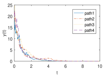
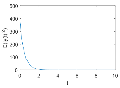
Figure 1: Four sample paths of the solution $y(t)$ and the sample mean of $|y(t)|^{2}$ for $50$ sample points for the system (5.19) for $t\in[0,10]$ with the time step $\Delta=0.02$.

Taking the conditional expectation on both sides and using the Hölder inequality, we obtain

$$\mathbb{E}^{1}\left[\mathbb{L}V(y(t),y(t-0.4),\mu_{t})\right]\leq-\frac{5}{2}\mathbb{E}^{1}|y(t)|^{2}+\frac{1}{2}\mathbb{E}^{1}|y(t-0.4)|^{2},$$

which implies (5.17) holds with $\lambda_{1}=5/2,\lambda_{2}=1/2$. Notice that $\bar{\delta}=0$. Then by (5.14), we compute that $\lambda=0.8927$. Then by Theorem 5.1, system (5.19) is mean square exponentially stable, i.e. $\limsup_{t\rightarrow\infty}\log[\mathbb{E}|X(t)|^{2}]/{t}\leq-0.8927.$ In order to have a feeling of the stability property, we simulate (5.19) using MATLAB with the time step $\Delta=0.02$. Figure 1 depicts four sample paths of the solution $y(t)$ and the sample mean of $|y(t)|^{2}$ for $50$ sample points for the system (5.19) for $t\in[0,10]$.

6 Delay feedback control for the McKean-Vlasov SDEs with common noise

This section is devoted to designing the control function for the McKean-Vlasov SDEs with common noise (1.1) to be bounded in the infinite horizon and to be mean square exponentially stable, i.e., to design a control term $u(t,X(t-\tau))$, in which $\tau$ is the time lag between the time when the observations for the state are made and the time when the feedback control reaches the system, such that the solution of the controlled system

$$\begin{aligned} \mathrm{d}X(t)&=\big{[}f\left(t,X(t),\mathcal{L}^{1}(X(t))\right)+u(t,X(t-\tau))\big{]}\mathrm{d}t+g\left(t,X(t),\mathcal{L}^{1}(X(t))\right)\mathrm{d}B_{t}\\ &\quad+g^{0}\left(t,X(t),\mathcal{L}^{1}(X(t))\right)\mathrm{d}B_{t}^{0},\end{aligned}$$ (6.1)

with the coefficients functions $f$, $g$ and $g^{0}$ satisfying the Lipschitz condition becomes bounded in the infinite horizon or stable. Here the initial value of (6.1) is $X(t)=X(0),-\tau\leq t\leq 0$, where $X(0)$ is $\mathcal{F}_{0}^{1}$-measurable and is the initial value of (1.1) satisfying that $\mathbb{E}|X(0)|^{p}<\infty~{}(p\geq 4)$. We will use the feedback control function with a simple form $u(t,x)=-\alpha x$ for $(x,t)\in\mathbb{R}^{d}\times\mathbb{R}_{+}$ where $\alpha$ is a positive constant.

With the purpose of dealing with the asymptotic property of the McKean-Vlasov SDDEs with common noise (6.1), we define two segments $\bar{X}_{t}:=\{X(t+\theta):-2\tau\leq\theta\leq 0\}$ and $\bar{\mu}_{t}:=\{\mu_{t+\theta}:-\tau\leq\theta\leq 0\}$ for $t\geq 0$. For the well definition of $\bar{X}_{t}$ and $\bar{\mu}_{t}$, we let $X(\theta):=X(0)$ for $-2\tau\leq\theta\leq-\tau$ and $\mu_{\theta}:=\mu_{0}$ for $-\tau\leq\theta\leq 0$ where $\mu_{t}:=\mathcal{L}^{1}(X(t))$ for $t\geq 0$. To control the derivation from the time delay in the mean square, i.e. the value of $\mathbb{E}|X(t)-X(t-\tau)|^{2}$, we define an auxiliary functional

$$\begin{aligned} I(\bar{X}_{t},\bar{\mu}_{t},t):=\int_{-\tau}^{0}\int_{t+r}^{t}\big{[}&\tau|f(z,X(z),\mu_{z})-\alpha X(z-\tau)|^{2}+\|g(z,X(z),\mu_{z})\|^{2}\\ &+\|g^{0}(z,X(z),\mu_{z})\|^{2}\big{]}\mathrm{d}z\mathrm{d}r,\end{aligned}$$ (6.2)

in which $f(t,x,\mu)=f(0,x,\mu)$, $g(t,x,\mu)=g(0,x,\mu)$ and $g^{0}(t,x,\mu)=g^{0}(0,x,\mu)$ for $(t,x,\mu)\in[-2\tau,0]\times\mathbb{R}^{d}\times\mathcal{P}_{2}(\mathbb{R}^{d})$. For simplicity, we write $I(t):=I(\bar{X}_{t},\bar{\mu}_{t},t)$. Then, the derivation principle of iterated integral gives

$$\mathrm{d}I(t)=I_{1}(t)\mathrm{d}t-I_{2}(t)\mathrm{d}t,$$ (6.3)

where

$$\begin{aligned} I_{1}(t)&=\!\tau\!\big{[}\tau|f(t,X(t),\mu_{t})\!-\!\alpha X(t\!-\!\tau)|^{2}\!+\!\|g(t,X(t),\mu_{t})\|^{2}\!+\!\|g^{0}(t,X(t),\mu_{t})\|^{2}\big{]}\\ I_{2}(t)&=\int_{-\tau}^{0}\big{[}\tau|f(t+r,X(t+r),\mu_{t+r})-\alpha X(t+r-\tau)|^{2}\\ &\quad\quad\quad+\|g(t+r,X(t+r),\mu_{t+r})\|^{2}+\|g^{0}(t+r,X(t+r),\mu_{t+r})\|^{2}\big{]}\mathrm{d}r.\end{aligned}$$ (6.4)

Changing the integration order, one derives that

$$I(t)\leq\tau I_{2}(t).$$ (6.5)

We go a further step to estimate the derivation from the time delay in the mean square. Making use of the Hölder inequality and the Itô isometry formula, one arrives at

$$\mathbb{E}|X(t)-X(t-\tau)|^{2}\leq 3\mathbb{E}\Big{[}\int_{t-\tau}^{t}\!\! \tau|f\left(s,X(s),\mu_{s}\right)\!-\!\alpha X(s\!-\!\tau)|^{2}\!+\!\|g\left(s,X(s),\mu_{s}\right)\|^{2}$$

$$+\|g^{0}\left(s,X(s),\mu_{s}\right)\|^{2}\mathrm{d}s\Big{]}\leq 3\mathbb{E}[I_{2}(t)].$$ (6.6)

6.1 Boundedness control

It is well known that the mean square moment of the global solution of the linear SDEs with common noise on $[0,\infty)$ may be unbounded on the infinite-time horizon [25]. Therefore, it is reasonable to design the control function $u(x(t-\tau)),t):=-\alpha x(t-\tau)$ such that the solution of the controlled system (6.1) becomes bounded in the mean square on $[0,\infty)$. For this purpose, we first give a hypothesis on the coefficients for equation (1.1).

Assumption 4.

There exist positive constants $\bar{K},\bar{E},\bar{L}_{1}$ and $\bar{L}_{2}$ such that for any $t\geq 0,x\in\mathbb{R}^{d}$, and $\mu\in\mathcal{P}_{2}\left(\mathbb{R}^{d}\right)$,

$$|f(t,x,\mu)|\vee\|g(t,x,\mu)\|\vee\|g^{0}(t,x,\mu)\|\leq\bar{K}(1+|x|+\mathbb{W}_{2}(\mu,\delta_{0})),$$

$$2x^{T}f(t,x,\mu)+\|g(t,x,\mu)\|^{2}+\|g^{0}(t,x,\mu)\|^{2}\leq\bar{E}+\bar{L}_{1}|x|^{2}+\bar{L}_{2}\mathbb{W}_{2}^{2}(\mu,\delta_{0}).$$

Under Assumption 4, the existence and uniqueness for the solutions of equation (1.1) and (6.1) are guaranteed by [9, Vol-II, Proposition 2.8] and Theorem 3.1, respectively.

Theorem 6.1.

Let Assumption 4 hold. Assume that $2\alpha>\bar{L}_{1}+\bar{L}_{2}$. If $0<\tau<\tau_{1}^{*}:=y_{1}\wedge y_{2}$, then the solution $X(t)$ of (6.1) has the property that

$$\sup_{0\leq t<\infty}\mathbb{E}|X(t)|^{2}<\infty,$$

where $y_{1}$ and $y_{2}$ are the unique positive roots of the following equations

$$\bar{\beta}_{1}(y)=\frac{(2\alpha-\bar{L}_{1}-\bar{L}_{2})^{2}}{96\alpha^{2}},\quad\iota_{1}(y)=\frac{1}{6},$$

$\bar{\beta}_{1}(\cdot)$ and $\iota_{1}(\cdot)$ are defined by (6.15) and (6.9), respectively.

Proof. Fix $0<\tau<\tau_{1}^{*}$. Define $V(t,\bar{X}_{t},\bar{\mu}_{t})=|X(t)|^{2}+\int_{\mathbb{R}^{d}}|x|^{2}\mu_{t}(\mathrm{d}x)+\sigma I(t),$ where $\sigma$ is a positive constant determined later. In order to estimate $V(t,\bar{X}_{t},\bar{\mu}_{t})$, we first analyze $I(t)$ defined by (6.2). By Assumption 4 and the definition of $I_{1}(t)$ in (6.4), we have

$$\begin{aligned} I_{1}(t)&\leq\tau\big{[}(6\bar{K}^{2}\tau+4\alpha^{2}\tau+6\bar{K}^{2})|X(t)|^{2}+(6\bar{K}^{2}\tau+6\bar{K}^{2})\mathbb{W}_{2}^{2}(\mu_{t},\delta_{0})\\ &\quad+4\alpha^{2}\tau|X(t)-X(t-\tau)|^{2}+(6\bar{K}^{2}\tau+6\bar{K}^{2})\big{]}.\end{aligned}$$ (6.7)

Inserting (6.7) into (6.3) gives that

$$\begin{aligned} \mathrm{d}I(t)&\!\leq\!\big{[}\beta_{1}(\tau)|X(t)|^{2}\!+\!\beta_{2}(\tau)\mathbb{E}^{1}[|X(t)|^{2}]\!+\!\iota_{1}(\tau)|X(t)\!-\!X(t\!-\!\tau)|^{2}\\ &\quad\!+\!\beta_{2}(\tau)\!-\!I_{2}(t)\big{]}\mathrm{d}t,\end{aligned}$$ (6.8)

where

$$\beta_{1}(y)=2y(y(3\bar{K}^{2}+2\alpha^{2})+3\bar{K}^{2}),~{}\beta_{2}(y)=2y(3\bar{K}^{2}y+3\bar{K}^{2}),~{}\iota_{1}(y)=4\alpha^{2}y^{2}.$$ (6.9)

We then estimate

$$U(X(t),\mu_{t}):=|X(t)|^{2}+\int_{\mathbb{R}^{d}}|x|^{2}\mu_{t}(\mathrm{d}x).$$ (6.10)

Applying Lemma 5.1 to $U(X(t),\mu_{t})$, and using the elementary inequality $2ab\leq\varepsilon a^{2}+(1/\varepsilon)b^{2}$ as well as Assumption 4, one obtains that

$$\begin{aligned} &\mathrm{d}U(X(t),\mu_{t})\\ &\leq\Big{[}\!-\!\Big{(}2\alpha\!-\!\bar{L}_{1}\!-\!\frac{\zeta}{2}\Big{)}|X(t)|^{2}\!+\!\frac{2\alpha^{2}}{\zeta}|X(t)\!-\!X(t\!-\!\tau)|^{2}\!-\!\Big{(}2\alpha\!-\!\bar{L}_{1}\!-\!2\bar{L}_{2}\!-\!\frac{\zeta}{2}\Big{)}\\ &\quad\times\!\mathbb{E}^{1}|X(t)|^{2}\!+\!\frac{2\alpha^{2}}{\zeta}\mathbb{E}^{1}|X(t)\!-\!X(t\!-\!\tau)|^{2}\!+\!2\bar{E}\Big{]}\mathrm{d}t\!+\!2X^{T}(t)g(t,X(t),\mu_{t})\mathrm{d}B_{t}\\ &\quad+2X^{T}(t)g^{0}(t,X(t),\mu_{t})\mathrm{d}B^{0}_{t}+\int_{\mathbb{R}^{d}}2z^{T}g^{0}(t,z,\mu_{t})\mu_{t}(\mathrm{d}z)\mathrm{d}B^{0}_{t}.\end{aligned}$$ (6.11)

It follows from (6.8) and (6.11) that for any $t\geq 0$,

$$\mathrm{d}V(t,\bar{X}_{t},\bar{\mu}_{t})$$

$$\leq\Big{[}-\Big{(}2\alpha-\bar{L}_{1}-\frac{\zeta}{2}-\sigma\beta_{1}(\tau)\Big{)}|X(t)|^{2}+\Big{(}\frac{2\alpha^{2}}{\zeta}+\sigma\iota_{1}(\tau)\Big{)}|X(t)-X(t-\tau)|^{2}$$

$$\quad-\Big{(}2\alpha-\bar{L}_{1}-2\bar{L}_{2}-\frac{\zeta}{2}-\sigma\beta_{2}(\tau)\Big{)}\mathbb{E}^{1}|X(t)|^{2}+\frac{2\alpha^{2}}{\zeta}\mathbb{E}^{1}|X(t)-X(t-\tau)|^{2}$$

$$\quad-\sigma I_{2}(t)+\sigma\beta_{2}(\tau)+2\bar{E}\Big{]}\mathrm{d}t+2X^{T}(t)g(t,X(t),\mu_{t})\mathrm{d}B_{t}$$

$$\quad+2X^{T}(t)g^{0}(t,X(t),\mu_{t})\mathrm{d}B^{0}_{t}+\mathbb{E}^{1}[2X^{T}(t)g^{0}(t,X(t),\mu_{t})]\mathrm{d}B^{0}_{t}.$$ (6.12)

By Lemma 5.1 and (6.1), one has

$$\begin{aligned} &\mathrm{d}e^{\gamma t}V(t,\bar{X}_{t},\bar{\mu}_{t})\\ &\leq e^{\gamma t}\Big{[}\!-\!\Big{(}2\alpha\!-\!\bar{L}_{1}\!-\!\frac{\zeta}{2}\!-\!\sigma\beta_{1}(\tau)\!-\!\gamma\Big{)}|X(t)|^{2}\!+\!\Big{(}\frac{2\alpha^{2}}{\zeta}\!+\!\sigma\iota_{1}(\tau)\Big{)}|X(t)\!-\!X(t\!-\!\tau)|^{2}\\ &\quad-\!\Big{(}2\alpha\!-\!\bar{L}_{1}\!-\!2\bar{L}_{2}\!-\!\frac{\zeta}{2}\!-\!\sigma\beta_{2}(\tau)\!-\!\gamma\Big{)}\mathbb{E}^{1}|X(t)|^{2}\!+\!\frac{2\alpha^{2}}{\zeta}\mathbb{E}^{1}|X(t)\!-\!X(t\!-\!\tau)|^{2}\\ &\quad-\sigma I_{2}(t)+\gamma\sigma I(t)+\sigma\beta_{2}(\tau)+2\bar{E}\Big{]}\mathrm{d}t+2e^{\gamma t}X^{T}(t)g(t,X(t),\mu_{t})\mathrm{d}B_{t}\\ &\quad+2e^{\gamma t}X^{T}(t)g^{0}(t,X(t),\mu_{t})\mathrm{d}B^{0}_{t}+\mathbb{E}^{1}[2e^{\gamma t}X^{T}(t)g^{0}(t,X(t),\mu_{t})]\mathrm{d}B^{0}_{t},\end{aligned}$$ (6.13)

where $\gamma$ is a positive constant defined later. Integrating and taking expectation on both sides of (6.13), we compute that

$$\begin{aligned} &\mathbb{E}[e^{\gamma t}V(t,\bar{X}_{t},\bar{\mu}_{t})]-\mathbb{E}[V(0,\bar{X}_{0},\mu_{0})]\\ &\leq\int_{0}^{t}\!e^{\gamma s}\Big{[}\!-\!\Big{(}4\alpha\!-\!2\bar{L}_{1}\!-\!2\bar{L}_{2}\!-\!\zeta\!-\!4\sigma\bar{\beta}_{1}(\tau)\!-\!2\gamma\Big{)}\mathbb{E}|X(s)|^{2}\!+\!\Big{(}\frac{4\alpha^{2}}{\zeta}\!+\!\sigma\iota_{1}(\tau)\Big{)}\\ &\quad\times\mathbb{E}|X(s)-X(s-\tau)|^{2}-\sigma\mathbb{E}I_{2}(s)+\gamma\sigma\mathbb{E}I(s)+\sigma\beta_{2}(\tau)+2\bar{E}\big{]}\mathrm{d}s,\end{aligned}$$ (6.14)

where

$$\bar{\beta}_{1}(y)=y(y(3\bar{K}^{2}+\alpha^{2})+3\bar{K}^{2}).$$ (6.15)

Then, combining (6.5), (6) and (6.14) shows that

$$\begin{aligned} &\mathbb{E}[e^{\gamma t}V(t,\bar{X}_{t},\bar{\mu}_{t})]\\ &\leq 2\mathbb{E}|X(0)|^{2}+\sigma\mathbb{E}[I(0)]+\int_{0}^{t}e^{\gamma s}\big{[}-(4\alpha-2\bar{L}_{1}-2\bar{L}_{2}-\zeta-4\sigma\bar{\beta}_{1}(\tau)-2\gamma)\\ &\quad\times\mathbb{E}|X(s)|^{2}-\Big{(}\sigma(1-3\iota_{1}(\tau))-\frac{12\alpha^{2}}{\zeta}-\gamma\sigma\tau\Big{)}\mathbb{E}I_{2}(s)+\sigma\beta_{2}(\tau)+2\bar{E}\big{]}\mathrm{d}s.\end{aligned}$$

Choose

$$\zeta=2\alpha-\bar{L}_{1}-\bar{L}_{2},\quad\mathrm{and}\quad\sigma=\frac{24\alpha^{2}}{\zeta}.$$ (6.16)

Due to the increasing property of $\bar{\beta}_{1}(y)$ and $\iota_{1}(y)$ in $y>0$ as well as the value of $\zeta$ and $\sigma$, we have $\beta_{2}(\tau)\leq(2\alpha-\bar{L}_{1}-\bar{L}_{2})/4$. Then we can find a sufficient small $\gamma$ such that

$$\mathbb{E}[e^{\gamma t}V(t,\bar{X}_{t},\bar{\mu}_{t})]\leq 2\mathbb{E}|X(0)|^{2}+\sigma\mathbb{E}[I(0)]+e^{\gamma t}\Big{[}\frac{\sigma(2\alpha-\bar{L}_{1}-\bar{L}_{2})+8\bar{E}}{4\gamma}\Big{]}.$$

Dividing $e^{\gamma t}$ on both side and using the definition of $V(t,\bar{X}_{t},\bar{\mu}_{t})$ yield that

$$\mathbb{E}[|X(t)|^{2}]\leq 2\mathbb{E}|X(0)|^{2}e^{-\gamma t}+\sigma\mathbb{E}[I(0)]e^{-\gamma t}+\frac{\sigma(2\alpha-\bar{L}_{1}-\bar{L}_{2})+8\bar{E}}{4\gamma}.$$

Therefore, the required assertion follows. ∎

6.2 Stabilization

In this subsection, we pay attention to giving the criteria of the stability of the controlled system (6.1). To ensure the trivial solution of (6.1), we replace Assumption 4 with the following Assumption:

Assumption 5.

There exist positive constants $\bar{K}_{1},\bar{K}_{2},\bar{L}_{1}$ and $\bar{L}_{2}$ such that for any $t\geq 0,x\in\mathbb{R}^{d}$, and $\mu\in\mathcal{P}_{2}\left(\mathbb{R}^{d}\right)$,

$$|f(t,x,\mu)|\vee\|g(t,x,\mu)\|\vee\|g^{0}(t,x,\mu)\|\leq\bar{K}_{1}|x|+\bar{K}_{2}\mathbb{W}_{2}(\mu,\delta_{0}),$$

$$2x^{T}f(t,x,\mu)+\|g(t,x,\mu)\|^{2}+\|g^{0}(t,x,\mu)\|^{2}\leq\bar{L}_{1}|x|^{2}+\bar{L}_{2}\mathbb{W}_{2}^{2}(\mu,\delta_{0}).$$

Theorem 6.2.

Let Assumption 5 hold. Assume that $2\alpha>\bar{L}_{1}+\bar{L}_{2}$. Then for any $0<\tau<\tau^{*}_{2}:=y_{3}\wedge y_{4}$, the solution $X(t)$ of (6.1) is exponentially stable in the mean square, i.e. there exists a positive constant $\gamma$ such that

$$\limsup_{t\rightarrow\infty}\frac{1}{t}\log[\mathbb{E}|X(t)|^{2}]\leq-\gamma,$$

where

$$\gamma=\min\left\{\frac{(2\alpha-\bar{L}_{1}-\bar{L}_{2})^{2}-24\alpha^{2}\bar{\beta}_{2}(\tau)}{4\alpha-2\bar{L}_{1}-2\bar{L}_{2}},\frac{1-6\iota_{2}(\tau)}{2\tau}\right\},$$ (6.17)

and $y_{3}$ and $y_{4}$ are the unique positive roots of the equalities

$$\bar{\beta}_{2}(y)=\frac{(2\alpha-\bar{L}_{1}-\bar{L}_{2})^{2}}{24\alpha^{2}},\quad\iota_{2}(y)=\frac{1}{6},$$ (6.18)

respectively, $\bar{\beta}_{2}(\cdot)$ and $\iota_{2}(\cdot)$ are defined by (6.25) and (6.20), respectively.

Proof. Fix $0<\tau<\tau^{*}_{2}$. Let $\mu_{t}:=\mathcal{L}^{1}(X(t))$. Making use of Assumption 5, we estimate $I(t)$ defined by (6.2)

$$\mathrm{d}I(t) \!\leq\!\big{[}\beta_{3}(\tau)|X(t)|^{2}\!+\!\beta_{4}(\tau)\mathbb{E}^{1}[|X(t)|^{2}]+\iota_{2}(\tau)|X(t)-X(t-\tau)|^{2}-I_{2}(t)\big{]}\mathrm{d}t,$$ (6.19)

where

$$\beta_{3}(y)=y(y(6\bar{K}_{1}^{2}+3\alpha^{2})+4\bar{K}_{1}^{2}),~{}\beta_{4}(y)=y(6\bar{K}_{2}^{2}y+4\bar{K}_{2}^{2}),~{}\iota_{2}(y)=3\alpha^{2}y^{2}.$$ (6.20)

Applying Lemma 5.1 to $U(X(t),\mu_{t})$ defined in (6.10), using the elementary inequality and Assumption 5, one computes that for $\zeta>0$,

$$\begin{aligned} &\mathrm{d}U(X(t),\mu_{t})\\ &\leq\Big{[}-\Big{(}2\alpha\!-\!\bar{L}_{1}\!-\!\frac{\zeta}{2}\Big{)}|X(t)|^{2}\!+\!\frac{2\alpha^{2}}{\zeta}|X(t)\!-\!X(t\!-\!\tau)|^{2}\!-\!\Big{(}2\alpha\!-\!\bar{L}_{1}\!-\!2\bar{L}_{2}\!-\!\frac{\zeta}{2}\Big{)}\\ &\quad\times\mathbb{E}^{1}[|X(t)|^{2}]+\frac{2\alpha^{2}}{\zeta}\mathbb{E}^{1}[|X(t)-X(t-\tau)|^{2}]\Big{]}\mathrm{d}t+2X^{T}(t)g(t,X(t),\mu_{t})\mathrm{d}B_{t}\\ &\quad+2X^{T}(t)g^{0}(t,X(t),\mu_{t})\mathrm{d}B^{0}_{t}+\int_{\mathbb{R}^{d}}2z^{T}g^{0}(t,z,\mu_{t})\mu_{t}(\mathrm{d}z)\mathrm{d}B^{0}_{t}.\end{aligned}$$ (6.21)

It follows from (6.19) and (6.21) that for any $t\geq 0$,

$$\mathrm{d}V(t,\bar{X}_{t},\bar{\mu}_{t})$$

$$\leq\big{[}-(2\alpha-\bar{L}_{1}-\frac{\zeta}{2}-\sigma\beta_{3}(\tau))|X(t)|^{2}+\Big{(}\frac{2\alpha^{2}}{\zeta}+\sigma\iota_{2}(\tau)\Big{)}|X(t)-X(t-\tau)|^{2}$$

$$\quad-(2\alpha-\bar{L}_{1}-2\bar{L}_{2}-\frac{\zeta}{2}-\sigma\beta_{4}(\tau))\mathbb{E}^{1}[|X(t)|^{2}]+\frac{2\alpha^{2}}{\zeta}\mathbb{E}^{1}[|X(t)-X(t-\tau)|^{2}]$$

$$\quad-\sigma I_{2}(t)\Big{]}\mathrm{d}t+2X^{T}(t)g(t,X(t),\mu_{t})\mathrm{d}B_{t}+2X^{T}(t)g^{0}(t,X(t),\mu_{t})\mathrm{d}B^{0}_{t}$$

$$\quad+\mathbb{E}^{1}[2X^{T}(t)g^{0}(t,X(t),\mu_{t})]\mathrm{d}B^{0}_{t}.$$ (6.22)

Then one obtains from Lemma 5.1 and (6.2) that

$$\begin{aligned} &\mathrm{d}[e^{\gamma t}V(t,\bar{X}_{t},\bar{\mu}_{t})]\\ &\leq e^{\gamma t}\Big{[}\big{[}\!-\!(2\alpha\!-\!\bar{L}_{1}\!-\!\frac{\zeta}{2}\!-\!\sigma\beta_{3}(\tau)\!-\!\gamma)|X(t)|^{2}\!+\!\Big{(}\frac{2\alpha^{2}}{\zeta}\!+\!\sigma\iota_{2}(\tau)\Big{)}|X(t)\!-\!X(t\!-\!\tau)|^{2}\\ &\quad-\!(2\alpha\!-\!\bar{L}_{1}\!-\!2\bar{L}_{2}\!-\!\frac{\zeta}{2}\!-\!\sigma\beta_{4}(\tau)\!-\!\gamma)\mathbb{E}^{1}[|X(t)|^{2}]\!+\!\frac{2\alpha^{2}}{\zeta}\mathbb{E}^{1}[|X(t)\!-\!X(t\!-\!\tau)|^{2}]\\ &\quad-\sigma I_{2}(t)+\gamma\sigma I(t)\big{]}\mathrm{d}t+2X^{T}(t)g(t,X(t),\mu_{t})\mathrm{d}B_{t}\\ &\quad+2X^{T}(t)g^{0}(t,X(t),\mu_{t})\mathrm{d}B^{0}_{t}+\mathbb{E}^{1}[2X^{T}(t)g^{0}(t,X(t),\mu_{t})]\mathrm{d}B^{0}_{t}\Big{]},\end{aligned}$$ (6.23)

where $\gamma$ is defined in (6.17). Integrating and taking expectation on both sides of (6.23) as well as using (6.5) and (6) show that

$$\begin{aligned} &\mathbb{E}[e^{\gamma t}V(t,\bar{X}_{t},\bar{\mu}_{t})]\\ &\leq 2\mathbb{E}|X(0)|^{2}+\sigma\mathbb{E}[I(0)]+\int_{0}^{t}e^{\gamma s}\big{[}-(4\alpha-2\bar{L}_{1}-2\bar{L}_{2}-\zeta-\sigma\bar{\beta}_{2}(\tau)-2\gamma)\\ &\quad\times\mathbb{E}|X(s)|^{2}-(\sigma(1-3\iota_{2}(\tau))-\frac{12\alpha^{2}}{\zeta}-\gamma\sigma\tau)\mathbb{E}I_{2}(s)\big{]}\mathrm{d}s,\end{aligned}$$ (6.24)

where

$$\bar{\beta}_{2}(y)=y(y(6\bar{K}_{1}^{2}+6\bar{K}_{2}^{2}+3\alpha^{2})+4\bar{K}_{1}^{2}+4\bar{K}_{2}^{2}).$$ (6.25)

Choosing $\zeta$, $\sigma$ as (6.16), using the monotonic property of $\bar{\beta}_{2}(y)$ and $\iota_{2}(y)$ in $y>0$, as well as the definition of $\gamma$, and dividing $e^{\gamma t}$ on both sides of (6.24), one arrives at

$$\mathbb{E}[|X(t)|^{2}]\leq(2\mathbb{E}|X(0)|^{2}+\sigma\mathbb{E}[I(0)])e^{-\gamma t}.$$

The proof is therefore complete.∎

6.3 Example

We further give an example to illustrate the result of feedback control.

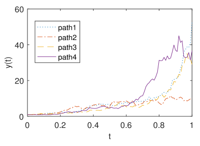
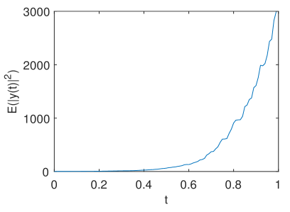
Figure 2: Four sample paths of the solution $y(t)$ and the sample mean of $|y(t)|^{2}$ for 50 sample points for the system (6.26) for $t\in[0,1]$ with the step size $\Delta=0.01$.

Example 6.1.

Consider the unstable Mckean-Vlasov SDE with common noise

$$\begin{aligned} \mathrm{d}y(t)&=\big{(}3y(t)+\mathbb{E}^{1}[y(t)]\big{)}\mathrm{d}t+\Big{(}y(t)+\frac{1}{2}\mathbb{E}^{1}[y(t)]\Big{)}\mathrm{d}B(t)\\ &\quad+\Big{(}y(t)+\frac{1}{2}\mathbb{E}^{1}[y(t)]\Big{)}\mathrm{d}B^{0}(t),\end{aligned}$$ (6.26)

with the initial value $y(0)=1$. We carry out the numerical simulation of (6.26) by MATLAB with the step size $\Delta=0.01$. Figure 2 depicts four sample paths of the solution $y(t)$ and the sample mean of $|y(t)|^{2}$ for 50 sample points for the system (6.26) for $t\in[0,1]$. One easily obtains that

$$|f(t,x,\mu)|\vee\|g(t,x,\mu)\|\vee\|g^{0}(t,x,\mu)\|\leq 3|x|+\mathbb{W}_{2}(\mu,\delta_{0}),$$

$$x^{T}f(t,x,\mu)+\|g(t,x,\mu)\|^{2}+\|g^{0}(t,x,\mu)\|^{2}\leq\frac{15}{2}|x|^{2}+\frac{5}{2}\mathbb{W}_{2}^{2}(\mu,\delta_{0}),$$

which means $\bar{K}_{1}=3$, $\bar{K}_{2}=1$, $\bar{L}_{1}=15/2$ and $\bar{L}_{2}=5/2$. Let $\alpha=10$. Then $2\alpha>\bar{L}_{1}+\bar{L}_{2}.$

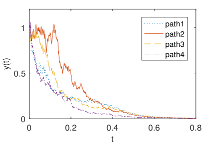
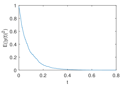
Figure 3: Four sample paths of the solution $y(t)$ and the sample mean of $|y(t)|^{2}$ for 50 sample points for the controlled system (6.27) for $t\in[0,0.8]$ with the step size $\Delta=0.001$.

The controlled system of the unstable Mckean-Vlasov SDE with common noise (6.26) becomes

$$\begin{aligned} \mathrm{d}y(t)&=\big{(}3y(t)-10y(t-\tau)+\mathbb{E}^{1}[y(t)]\big{)}\mathrm{d}t+\Big{(}y(t)+\frac{1}{2}\mathbb{E}^{1}[y(t)]\Big{)}\mathrm{d}B(t)\\ &\quad+\Big{(}y(t)+\frac{1}{2}\mathbb{E}^{1}[y(t)]\Big{)}\mathrm{d}B^{0}(t).\end{aligned}$$ (6.27)

By (6.18), (6.20) and (6.25), we obtain that $\tau^{*}_{2}\approx 0.0010321$. Choose $\tau=0.001$, then $\gamma=0.1568$. Then by Theorem 6.2, the solution of the controlled system (6.26) with initial value $y(0)=1$ has the property that $\limsup_{t\rightarrow\infty}\log[\mathbb{E}|X(t)|^{2}]/t\leq-0.1568.$ To show the stabilization intuitively, we intuitive (6.27) by MATLAB with the step size $\Delta=0.001$. Figure 3 depicts four sample paths of the solution $y(t)$ and the sample mean of $|y(t)|^{2}$ for 50 sample points for the controlled system (6.27) for $t\in[0,0.8]$.

7 Conclusions

In this paper, we study the existence and uniqueness of the solution of the McKean-Vlasov SFDEs with common noise and the conditional propagation of chaos. Making use of the Lyapunov method, we give sufficient criteria for the asymptotic boundedness and the exponential stability in $p$th moment $(p\geq 2)$ for the McKean-Vlasov SDDEs with common noise. Moreover, we design the delay feedback control function just depending on the state, which is more realistic and easy to implement to make the controlled system bounded and exponentially stable in the mean square and obtain the bound of the delay $\tau$.

References

- [1] K. J. ström and P. R. Kumar, Control: a perspective, Automatica, 50(2014), pp. 3-43.
- [2] J. Bao, J. Shao and D. Wei, Wellposedness of conditional McKean-Vlasov equations with singular drifts and regime-switching, Discrete Contin. Dyn. Syst. Ser. B, 28(2023), pp. 2911-2926.
- [3] K. Bahlali, M. Mezerdi and B. Mezerdi, Stability of McKean-Vlasov stochastic differential equations and applications, Stoch. Dyn., 20(2020), 2050007, pp. 19.
- [4] G. K. Basak, A. Bisi and M. K. Ghosh. Stability of a random diffusion with linear drift, J. Math. Anal. Appl., 202(1996), pp. 604-622.
- [5] P. Briand, P. Cardaliaguet, P.-E. Chaudru de Raynal and Y. Hu, Forward and Backward Stochastic Differential Equations with normal constraint in law, Stochastic Process. Appl., 130(2020), pp. 7021-7097.
- [6] R. Buckdahn, J. Li and J. Ma, A general conditional McKean-Vlasov stochastic differential equation, Ann. Appl. Probab. 33(2023), pp. 2004-2023.
- [7] M. Burzoni and L. Campi, Mean field games with absorption and common noise with a model of bank run, Stochastic Process. Appl. 164(2023), pp. 206-241.
- [8] P. Cardaliaguet, Notes on Mean Field Games (from Lion’s Lectures at College de France), https://www.ceremade.dauphine.fr/ cardaliaguet/MFG20130420.pdf.
- [9] R. Carmona and F. Delarue, Probabilistic Theory of Mean Field Games with Applications I-II, Springer, 2018.
- [10] R. Carmona, F. Delarue and D. Lacker, Mean field games with common noise, Ann. Probab., 44(2016), pp. 3740-3803.
- [11] M. Coghi and F. Flandoli, propagation of chaos for interacting particles subject to environmental noise, Ann. Appl. Probab., 26(2016), pp. 1407-1442.
- [12] M. Coghi and B. Gess, Stochastic nonlinear Fokker-Planck equations, Nonlinear Anal., 187(2019), pp. 259-278.
- [13] J. Cui, S. Liu and H. Zhou, Wasserstein Hamiltonian flow with common noise on graph, SIAM J. Appl. Math., 83(2023), pp. 484-509.
- [14] X. Ding and H. Qiao, Stability for stochastic McKean-Vlasov equations with non-Lipschitz coefficients, SIAM J. Control Optim., 59(2021), pp. 887-905.
- [15] N. Fournier and A. Guillin, On the rate of convergence in Wasserstein distance of the empirical measure, Probab. Theory Related Fields, 162(2015), pp. 707-738.
- [16] P. Graber, Linear quadratic mean field type control and mean field games with common noise, with application to production of an exhaustible resource, Appl. Math. Optim., 74(2016), pp. 459-486.
- [17] D. Gomes, J. Gutierrez and M. Laurire, Machine learning architectures for price formation models, Appl. Math. Optim., 88(2023), Paper No. 23, 41 pp.
- [18] W. R. P. Hammersley, D. Sika and L. Szpruch, Weak existence and uniqueness for McKean-Vlasov SDEs with common noise, Ann. Probab., 49(2021), pp. 527-555.
- [19] X. Huang, M. Röckner and F.-Y. Wang, Nonlinear Fokker-Planck equations for probability measures on path space and path-distribution dependent SDEs, Discrete Contin. Dyn. Syst., 39(2019), pp. 3017-3035.
- [20] V. N. Kolokoltsov and M. Troeva, On the mean field games with common noise and the McKean-Vlasov SPDEs, arXiv: 1506.0459
- [21] C. Kumar, Neelima, C. Reisinger and W. Stockinger, Well-posedness and tamed schemes for McKean-Vlasov equations with common noise, Ann. Appl. Probab., 32(2022), pp. 3283-3330.
- [22] T. G. Kurtz and J. Xiong, Particle representations for a class of nonlinear SPDEs, Stochas tic Process. Appl., 83(1999), pp. 103-126.
- [23] D. Lacker and L. Le Flem, Closed-loop convergence for mean field games with common noise, Ann. Appl. Probab., 33(2023), pp. 2681-2733.
- [24] M. Li, N. Li and Z. Wu, Dynamic optimization problems for mean-field stochastic large-population systems, ESAIM Control Optim. Calc. Var. 28 (2022), Paper No. 49, 25 pp.
- [25] X. Li, X. Mao, D. S. Mukama and C. Yuan, Delay feedback control for switching diffusion systems based on discrete time observations, SIAM J. Control Optim., 58 (2020), pp. 2900-2926.
- [26] X. Mao, Stochastic Differential Equations and Applications, 2nd ed., Horwood, Chichester, England, 2008.
- [27] X. Mao, J. Lam and L. Huang, Stabilisation of hybrid stochastic differential equations by delay feedback control, Systems Control Lett., 57(2008), pp. 927-935.
- [28] H. P. McKean, A class of Markov processes associated with nonlinear parabolic equations, Proc. Nat. Acad. Sci. U.S.A., 56(1966), pp. 1907-1911.
- [29] R. Maillet, A note on the Long-Time behaviour of Stochastic McKean-Vlasov Equations with common noise, arXiv:2306.16130
- [30] M. L. Rosinberg, T. Munakata and G. Tarjus, Stochastic thermodynamics of Langevinsystems under time-delayed feedback control: Second-law-like inequalities, Phys. Rev. E, 91 (2015), pp. 042114.
- [31] J. Shao, T. Tian and S. Wang, Conditional McKean-Vlasov SDEs with jumps and Markovian regime-switching: wellposedness, propagation of chaos, averaging principle, arXiv: 2301.08029.
- [32] J. Shao and D. Wei, Propagation of chaos and conditional McKean-Vlasov SDEs with regime-switching, Front. Math. China, 17(2022), pp. 731-746.
- [33] M. Sun, J. Lam, S. Xu and Y. Zou, Robust exponential stabilization for Markovian jump systems with mode-dependent input delay, Automatica, 43(2007), pp. 1799-1807.
- [34] D. ika and L. Szpruch, Gradient flows for regularized stochastic control problems, arXiv:2006.05956v4.
- [35] Y. V. Vuong, M. Hauray and E. Pardoux, Conditional propagation of chaos in a spatial stochastic epidemic model with common noise, Stoch. Partial Differ. Equ. Anal. Comput., 10(2022), pp. 1180-1210.
- [36] F.-Y. Wang, Distribution dependent SDEs for Landau type equations, Stochastic Process. Appl., 128(2018), pp. 595-621.
- [37] H. Wu, J. Hu, S. Gao and C. Yuan, Stabilization of stochastic McKean-Vlasov equations with feedback control based on discrete-time state observation, SIAM J. Control Optim., 60(2022), pp. 2884-2901.
- [38] F. Wu, F. Xi and C. Zhu, On a class of McKean-Vlasov stochastic functional differential equations with applications, J. Differential Equations, 371(2023), pp. 31-49.