Emergence of new topological gapless phases in the modified square-lattice Kitaev model

Abstract

We investigate emergent topological gapless phases in the square-lattice Kitaev model with additional hopping terms. In the presence of nearest-neighbor hopping only, the model is known to exhibit gapless phases with two topological gapless points. When the strength of the newly added next-nearest-neighbor hopping is smaller than a certain value, qualitatively the same phase diagram persists. We find that further increase of the extra hopping results in a new topological phase with four gapless points. We construct a phase diagram to clarify the regions of emergent topological gapless phases as well as topologically trivial ones in the space of the chemical potential and the next-nearest-neighbor hopping strength. We examine the evolution of the gapless phases in the energy dispersions of the bulk as the chemical potential varies. The topological properties of the gapless phases are characterized by the winding numbers of the present gapless points. We also consider the ribbon geometry to examine the corresponding topological edge states. It is revealed that Majorana-fermion edge modes exist as flat bands in topological gapless phases. We also perform the analytical calculation as to Majorana-fermion zero-energy modes and discuss its implications on the numerical results.

I Introduction

Topological properties of condensed matter have emerged as a new paradigm for classifying materials Hasan and Kane (2010); Wen (1995). They have attracted intense interests in view of their robustness against any continuous deformation. Topological insulators and topological superconductors are prototypes for interesting topological materials which have topologically nontrivial gapped phases. Topological insulators exhibit an insulating gap in the bulk and host gapless surface states preserved by time-reversal symmetry Hasan and Kane (2010). Topological superconductors have a pairing gap in the bulk and remarkably manifest Majorana particles on the surface attributed to particle-hole symmetry in the system Qi and Zhang (2011); Das Sarma (2023).

Majorana fermion is a particle which is its own antiparticle, suggested as real solutions of the Dirac equation by Ettore Majorana Alicea (2012); Beenakker (2013); Das Sarma (2023). In high energy physics neutrinos may be a candidate for Majorana fermions and experiments to demonstrate it have been still ongoing. Majorana particles are also of interest in condensed matter physics and they are proposed to be created as quasiparticles which are a linear combination of electrons and holes with equal weights Alicea (2012); Beenakker (2013); Stanescu and Tewari (2013); Elliott and Franz (2015); Sato and Fujimoto (2016); Das Sarma (2023). Researches on the realization of Majorana fermions have been performed intensively since Majorana fermions are promising candidates for topological qubits in fault-tolerant quantum computing. The experimental realization of Majorana modes in various platforms of superconductor has been under intensive researches but the obvious manifestation of Majorana edge modes is still in controversy Law et al. (2009); Mourik et al. (2012); He et al. (2017); Zhang et al. (2018); Nayak et al. (2008); Das Sarma (2023).

Theoretically it was shown that one-dimensional superconductor can host unpaired Majorana zero modes at the ends Kitaev (2001). The existence of the Majorana zero modes depends on $\mathbb{Z}_{2}$-type topological invariant of the one-dimensional superconductor. Two-dimensional topological superconductors in $\mathbb{Z}$-type integer classification host Majorana chiral edge modes and the integer topological invariant indicates the number of the edge modes. The simplest of these models is the spinless two-dimensional superconductors with $p_{x}+ip_{y}$ symmetry. This model hosts Majorana zero modes at the core of the vortex as well as Majorana chiral modes on the boundaries Read and Green (2000).

The search for Majorana zero modes has been conducted in topologically trivial superconductors as well. Majorana zero modes have been proposed to be realized in a two-dimensional superconducting Dirac semimetal with trivial bulk topology Chan et al. (2017). It was also pointed out that a Hopf invariant can protect Majorana zero modes in superconductors without chiral edge modes Yan et al. (2017). It has also been shown that two-dimensional topological insulators can exhibit Majorana zero modes at each corner when they are in the proximity with $d$-wave Yan et al. (2018) or $s_{\pm}$-wave Wang et al. (2018) superconductors. Topological gapless phases, which occur in topologically trivial superconductors described by the square-lattice Kitaev model, were also reported to display Majorana fermions in the form of a flat band Wang et al. (2017); Zhang et al. (2019). At the edges such flat bands connect two gapless points of opposite chirality in the bulk Ryu and Hatsugai (2002); Delplace et al. (2011); Chiu and Schnyder (2014); Zhang and Song (2020) which are preserved by the topological invariant of the model Matsuura et al. (2013).

In this work, we extend the square-lattice Kitaev model to explore the possibility of newly emergent gapless phases. For this purpose, we employ the modified square-lattice Kitaev model by adding next-nearest-neighbor hopping terms to the original model. In the earlier study Wang et al. (2017), the model with extra diagonal hopping was considered, leading to the conclusion that it does not give rise to any qualitatively different topological feature. We here find that topological gapless phases of a new type emerge from the introduction of extra next-nearest-neighbor hopping when it is imposed in the other diagonal direction. We perform the detailed analysis of the new topological phases in view of the phase boundary, the bulk energy dispersions, and Majorana zero-energy flat bands in the ribbon geometry. The rich physics of Majorana fermions in the modified square-lattice Kitaev model is also revealed in an analytical way.

II Modified square-lattice Kitaev model

II.1 Model

Square-lattice Kitaev model represents two-dimensional spinless superconductors with $p$-wave symmetryLi et al. (2006); Wang et al. (2017); Zhang et al. (2019), which is a two-dimensional generalization of the one-dimensional spinless fermionic HamiltonianLieb et al. (1961); Kitaev (2001). We consider the modified square-lattice Kitaev model which includes additional second nearest neighbor hopping terms. The Hamiltonian of the modified square-lattice Kitaev model is given by

$$\begin{split}H=&-t\sum_{\bm{r},\bm{a}}\left(c^{\dagger}_{\bm{r}}c_{\bm{r}+\bm{a}}+c^{\dagger}_{\bm{r}+\bm{a}}c_{\bm{r}}\right)-\Delta\sum_{\bm{r},\bm{a}}\left(c_{\bm{r}}c_{\bm{r}+\bm{a}}+c^{\dagger}_{\bm{r}+\bm{a}}c^{\dagger}_{\bm{r}}\right)\\ &-t^{\prime}\sum_{\bm{r}}\left(c^{\dagger}_{\bm{r}}c_{\bm{r}+\bm{b}}+c^{\dagger}_{\bm{r}+\bm{b}}c_{\bm{r}}\right)+\mu\sum_{\bm{r}}\left(2c^{\dagger}_{\bm{r}}c_{\bm{r}}-1\right),\end{split}$$ (1)

where $c^{\dagger}_{\bm{r}}$($c_{\bm{r}}$) is the creation(annihilation) operators of an electron at site $\bm{r}$ on the square lattice of $N$ lattice points. The first summation represents the hopping of strength $t$ between nearest neighbor sites. The second summation denotes Cooper pairing with $p$-wave symmetry, where $\Delta$ is an isotropic order parameter assumed to be real. The additional hopping terms of hopping amplitude $t^{\prime}$ are introduced in the third summation, where $\bm{b}\equiv a\bm{\hat{i}}-a\bm{\hat{j}}$ with $a$ being the lattice constant and $\bm{\hat{i}}(\bm{\hat{j}})$ being a unit vector in $x\left(y\right)$ direction. The last summation arises from chemical potential $\mu$. Throughout the paper We write all the energy quantities and the length scales in units of $t$ and $a$, respectively.

In order to examine the bulk phase we assume the periodic boundary conditions in both $x$ and $y$ directions. Taking the Fourier transformation on the fermion annihilation operators as

$$c_{\bm{r}}=\frac{1}{\sqrt{N}}\sum_{\bm{k}}c_{\bm{k}}e^{i\bm{k}\cdot\bm{r}},$$ (2)

we obtain the Hamiltonian of the form

$$H=\sum_{\bm{k}} \bigg{[}2\big{\{}\mu-t\left(\cos{k_{x}}+\cos{k_{y}}\right)-2t^{\prime}\cos(k_{x}{-}k_{y})\big{\}}c^{\dagger}_{\bm{k}}c_{\bm{k}}$$

$$-i\Delta\left(\sin{k_{x}}+\sin{k_{y}}\right)\left(c^{\dagger}_{\bm{k}}c^{\dagger}_{-\bm{k}}+c_{\bm{k}}c_{-\bm{k}}\right)-\mu\bigg{]}.$$ (3)

It can be expressed in terms of $\Psi_{\bm{k}}\equiv\small(\begin{array}[]{cc}c_{\bm{k}}&c^{\dagger}_{-\bm{k}}\end{array}\small)^{\dagger}$

$$H= \sum_{\bm{k}}\Psi_{\bm{k}}^{\dagger}\bm{h}_{\bm{k}}\Psi_{\bm{k}}$$

with

$$\bm{h}_{\bm{k}}\equiv \begin{pmatrix}-\mu+t\left(\cos{k_{x}}+\cos{k_{y}}\right)+t^{\prime}\cos{\left(k_{x}-k_{y}\right)}&-i\Delta\left(\sin{k_{x}}+\sin{k_{y}}\right)\\ i\Delta\left(\sin{k_{x}}+\sin{k_{y}}\right)&\mu-t\left(\cos{k_{x}}+\cos{k_{y}}\right)-t^{\prime}\cos{\left(k_{x}-k_{y}\right)}\end{pmatrix}.$$ (4)

The eigenvalues of $\bm{h}_{\bm{k}}$ provide quasiparticle eigenenergies $\pm\epsilon_{\bm{k}}$ with

$$\epsilon_{\bm{k}}\equiv\sqrt{\{-\mu+t\left(\cos{k_{x}}+\cos{k_{y}}\right)+t^{\prime}\cos{\left(k_{x}-k_{y}\right)}\}^{2}+\Delta^{2}\left(\sin{k_{x}}+\sin{k_{y}}\right)^{2}}.$$ (5)

II.2 Construction of phase diagram

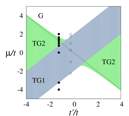
Figure 1: Phase diagram of the modified square-lattice Kitaev model characterized by the number of gapless points on the $\mu$-$t^{\prime}$ plane. ‘G’, ‘TG1’, and ‘TG2’ regions indicate gapful phase, gapless phase with a pair of gapless points, and gapless phase with two pairs of gapless points, respectively. The dotted line on $\mu=-t^{\prime}$ is the boundary where the topological property of gapless points changes. The empty circles at $t^{\prime}=-0.25t$ and the filled circles at $t^{\prime}=-1.25t$ are the representative systems whose properties are presented in subsequent sections.

The position of gapless points are determined by the condition $\epsilon_{\bm{k}}=0$,

$$\Delta\left(\sin{k_{x}}+\sin{k_{y}}\right)=0,$$ (6)

$$\mu-t\left(\cos{k_{x}}+\cos{k_{y}}\right)-t^{\prime}\cos(k_{x}-k_{y})=0.$$ (7)

The former equation yields two kinds of locations

$$k_{y}=-k_{x},$$ (8)

or

$$k_{y}=k_{x}+\pi,$$ (9)

where $k_{x}$ and $k_{y}$ are defined modulo $2\pi$ in the interval $[-\pi,\pi]$. The insertion of Eq. (8) into Eq. (7) leads to a quadratic equation of $\cos{k_{x}}$

$$-2t^{\prime}\cos^{2}{k_{x}}-2t\cos{k_{x}}+\mu+t^{\prime}=0,$$ (10)

yielding two formal solutions for $\cos{k_{x}}$

$$\chi_{\pm}\equiv\frac{-t\pm\sqrt{t^{2}+2t^{\prime}\left(\mu+t^{\prime}\right)}}{2t^{\prime}}.$$ (11)

A pair of gapless points

$$k_{x}=-k_{y}=\pm\arccos{\chi_{+}}$$ (12)

are guaranteed to exist in the condition $|\chi_{+}|<1$, which corresponds to the region $-f(-t^{\prime})<\mu<f(t^{\prime})$ with

$$\displaystyle f(x)\equiv\left\{\begin{array}[]{cc}\displaystyle-x-\frac{t^{2}}{2x}&\displaystyle\hbox{for }x<-\frac{1}{2}t,\\[8.53581pt] x+2t&\displaystyle\hbox{for }x>-\frac{1}{2}t.\end{array}\right.$$ (15)

We can find another pair of gapless points

$$k_{x}=-k_{y}=\pm\arccos{\chi_{-}}$$ (16)

if the system satisfies the condition $|\chi_{-}|<1$; the resulting region is

$$\begin{cases}\displaystyle t^{\prime}+2t<\mu<-\frac{t^{2}}{2t^{\prime}}-t^{\prime}\quad\displaystyle&\textrm{for}\quad\displaystyle t^{\prime}<-\frac{1}{2}t,\\ \displaystyle-\frac{t^{2}}{2t^{\prime}}-t^{\prime}<\mu<t^{\prime}-2t\quad&\textrm{for}\quad\displaystyle t^{\prime}>\frac{1}{2}t.\end{cases}$$ (17)

Equation (9) combined with Eq. (7) is satisfied on a line $\mu=-t^{\prime}$, where a nodal line $k_{y}=k_{x}+\pi$ of Eq. (9) exists on the momentum plane.

Summarizing the above results, we can construct the phase diagram shown in Fig. 1. In the region $\mu>f(t^{\prime})$ or $\mu<-f(-t^{\prime})$ the system lies in a normal gapped phase denoted by G in Fig. 1. In the region $t^{\prime}-2t<\mu<t^{\prime}+2t$ we observe a topological gapless phase with a pair of gapless points (TG1). In the intermediate region defined in Eq. (17) another topological gapless phase with two pairs of gapless points (TG2) emerges.

It is remarkable that the second gapless phase TG2 does not show up in the original square-lattice Kitaev model even when the second-nearest-neighbor hopping is introduced in the diagonal direction other than that considered in this work. The system exhibits straight nodal lines on the line $\mu=-t^{\prime}$, which is inside TG2 for $|t^{\prime}|>t$ and inside TG1 for $|t^{\prime}|<t$. In subsequent sections, we will give a description to how the phase evolves across the line.

In the remaining part, we will give a description mostly for $t^{\prime}<0$. We can always apply the same analysis to the system with $t^{\prime}>0$ by replacing $\mu$ and $t^{\prime}$ by $-\mu$ and $-t^{\prime}$ in the expressions for $t^{\prime}<0$.

II.3 Energy dispersions of quasiparticles

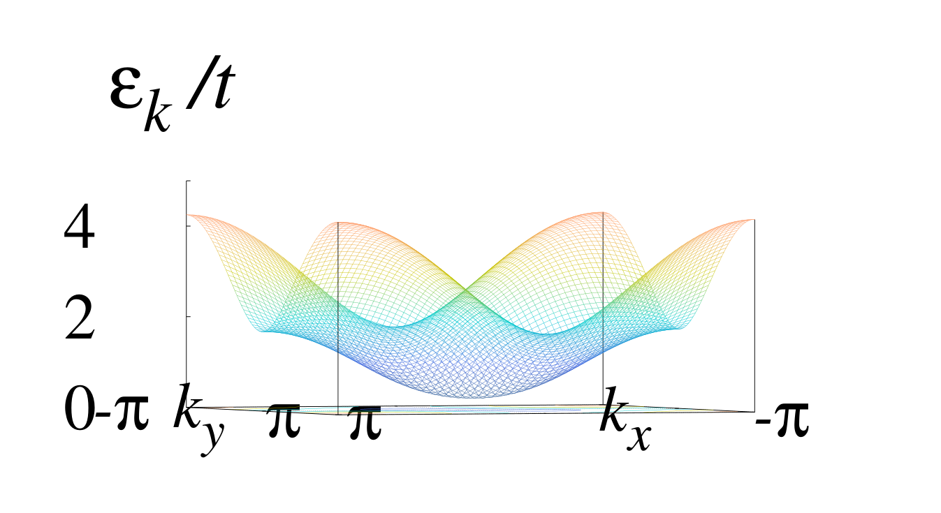
(a) $\mu=2t$

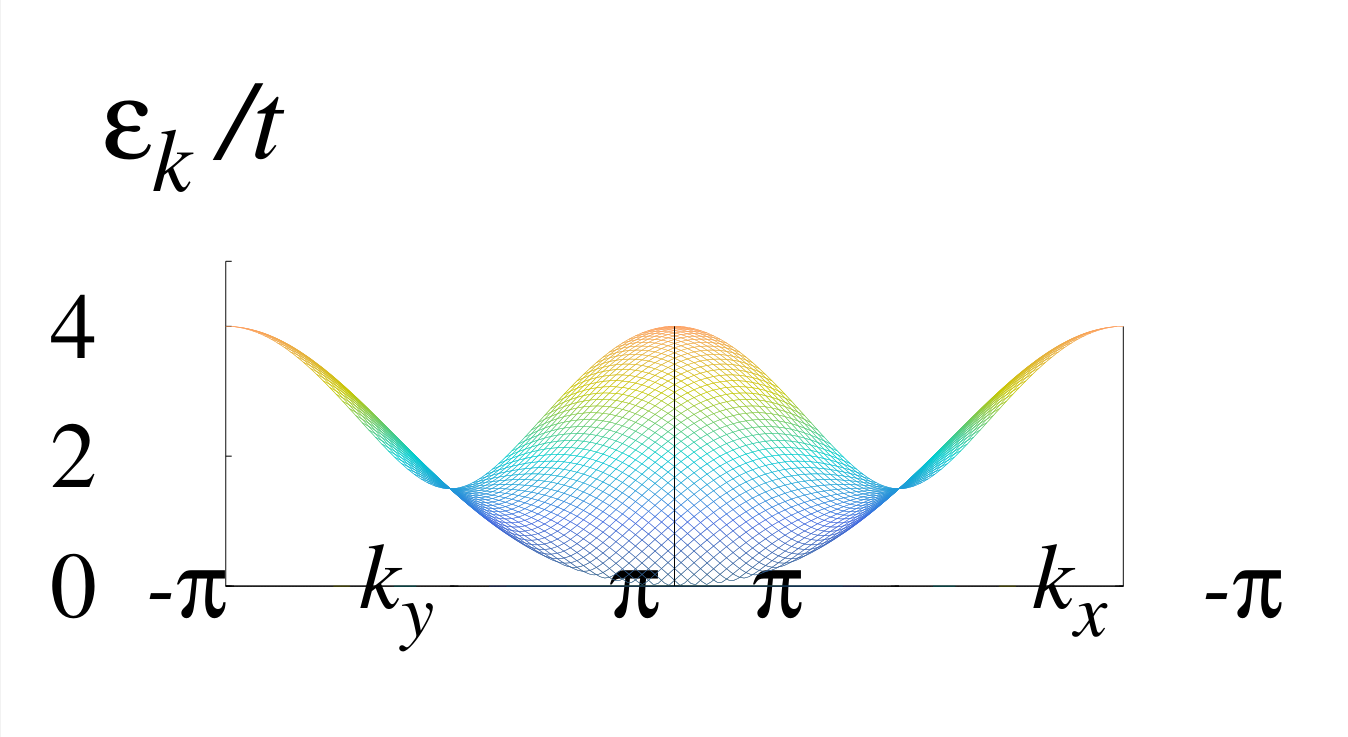
(b) $\mu=1.75t$

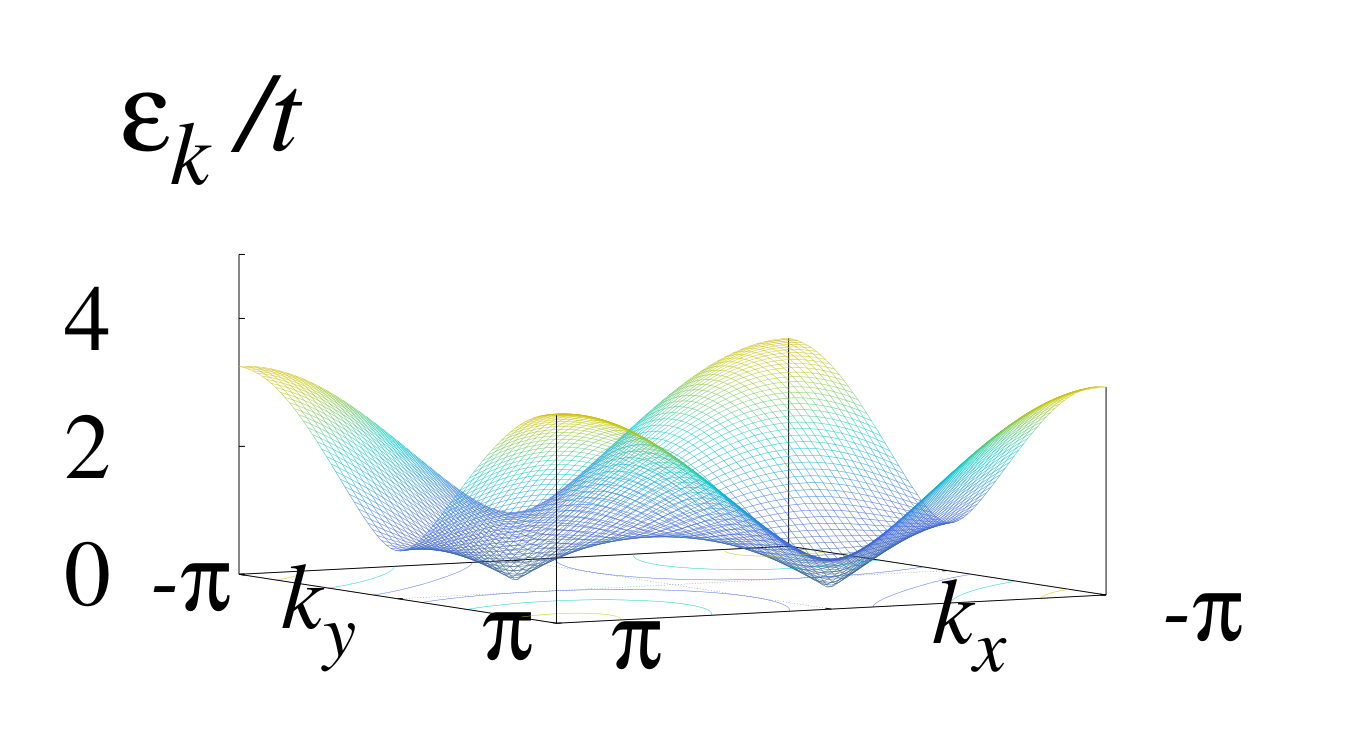
(c) $\mu=t$

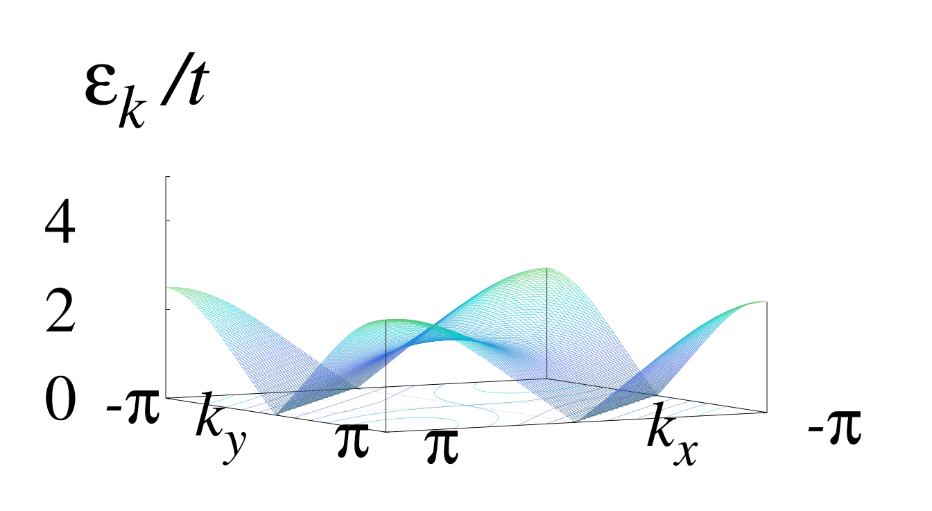
(d) $\mu=0.25t$

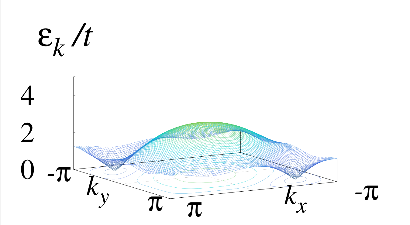
(e) $\mu=-t$

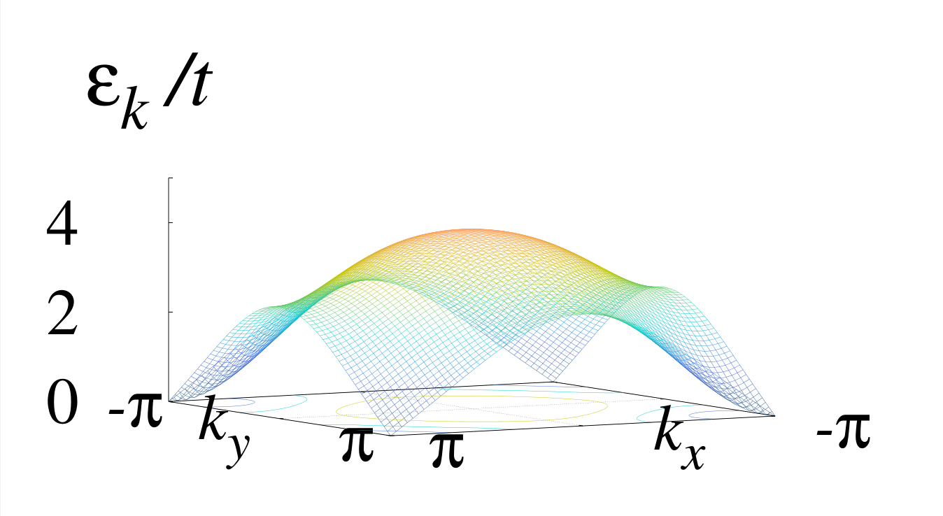
(f) $\mu=-2.25t$

Figure 2: Energy dispersions of the modified square-lattice Kitaev model for several values of chemical potential $\mu$ with $t^{\prime}=-0.25t$ and $\Delta=t$. The energy dispersions correspond to the empty circles on the line $t^{\prime}=-0.25t$ in Fig. 1.

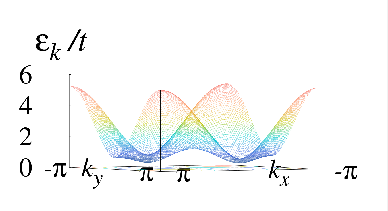
(a) $\mu=2t$

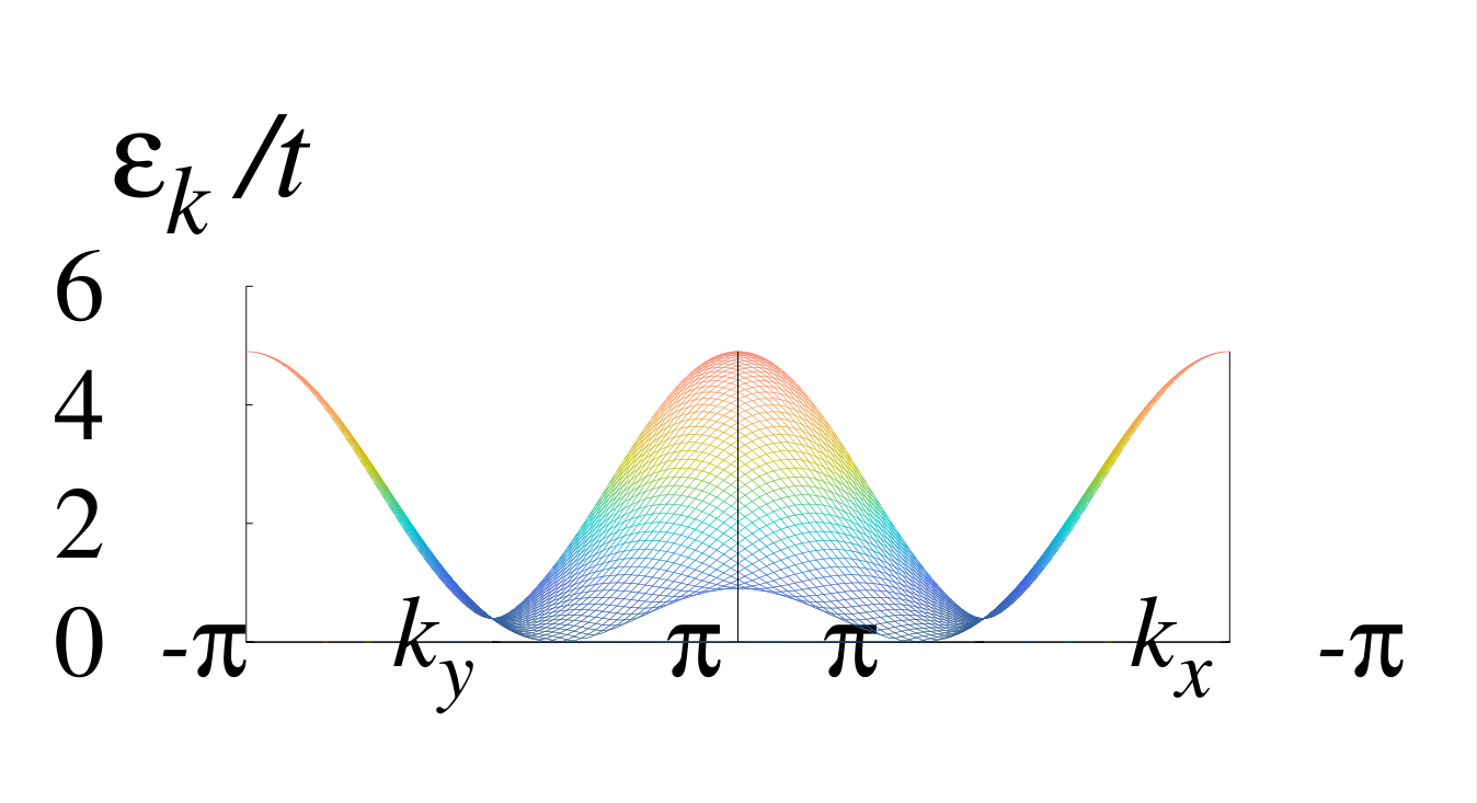
(b) $\mu=1.65t$

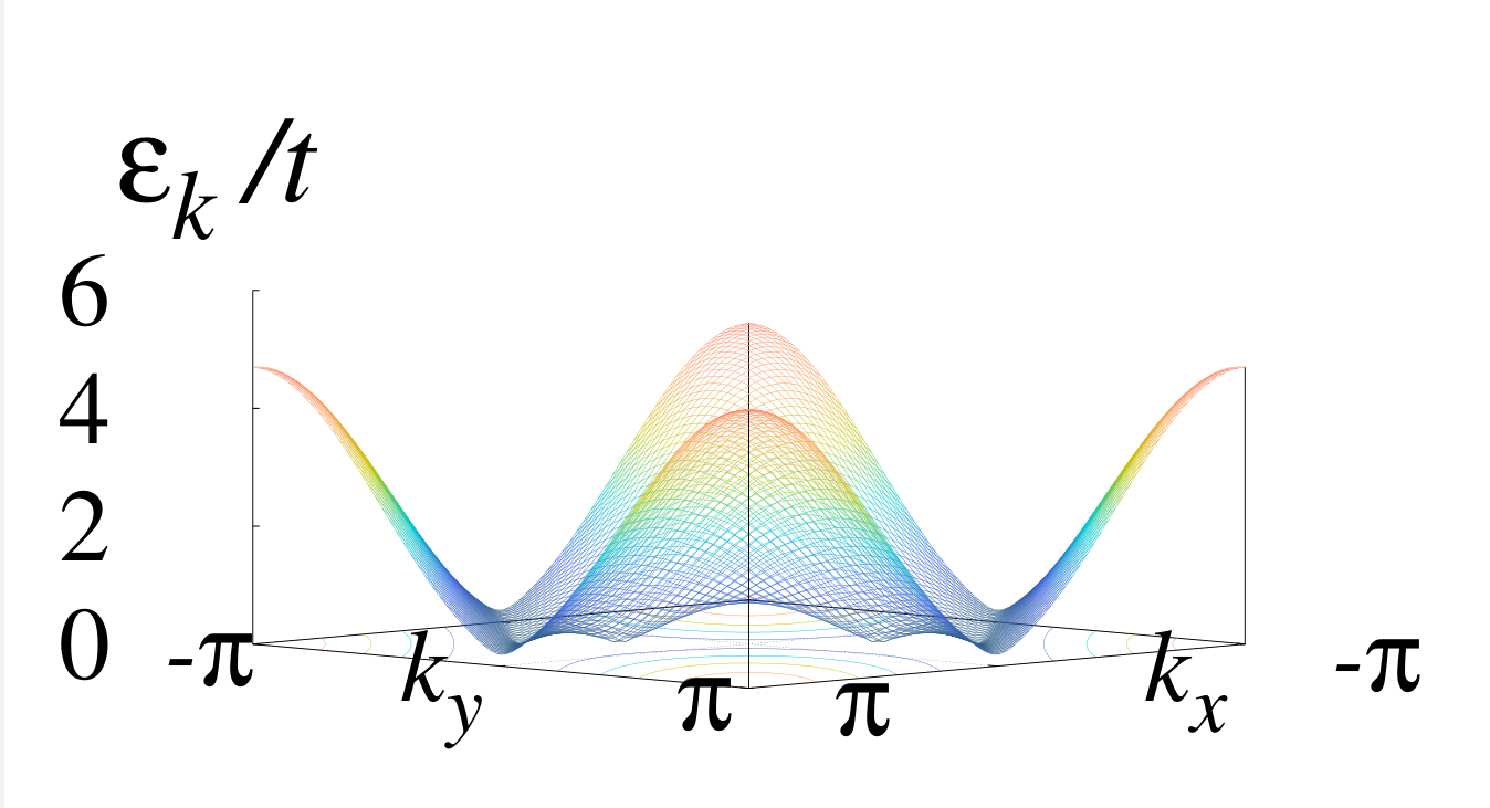
(c) $\mu=0.75t$

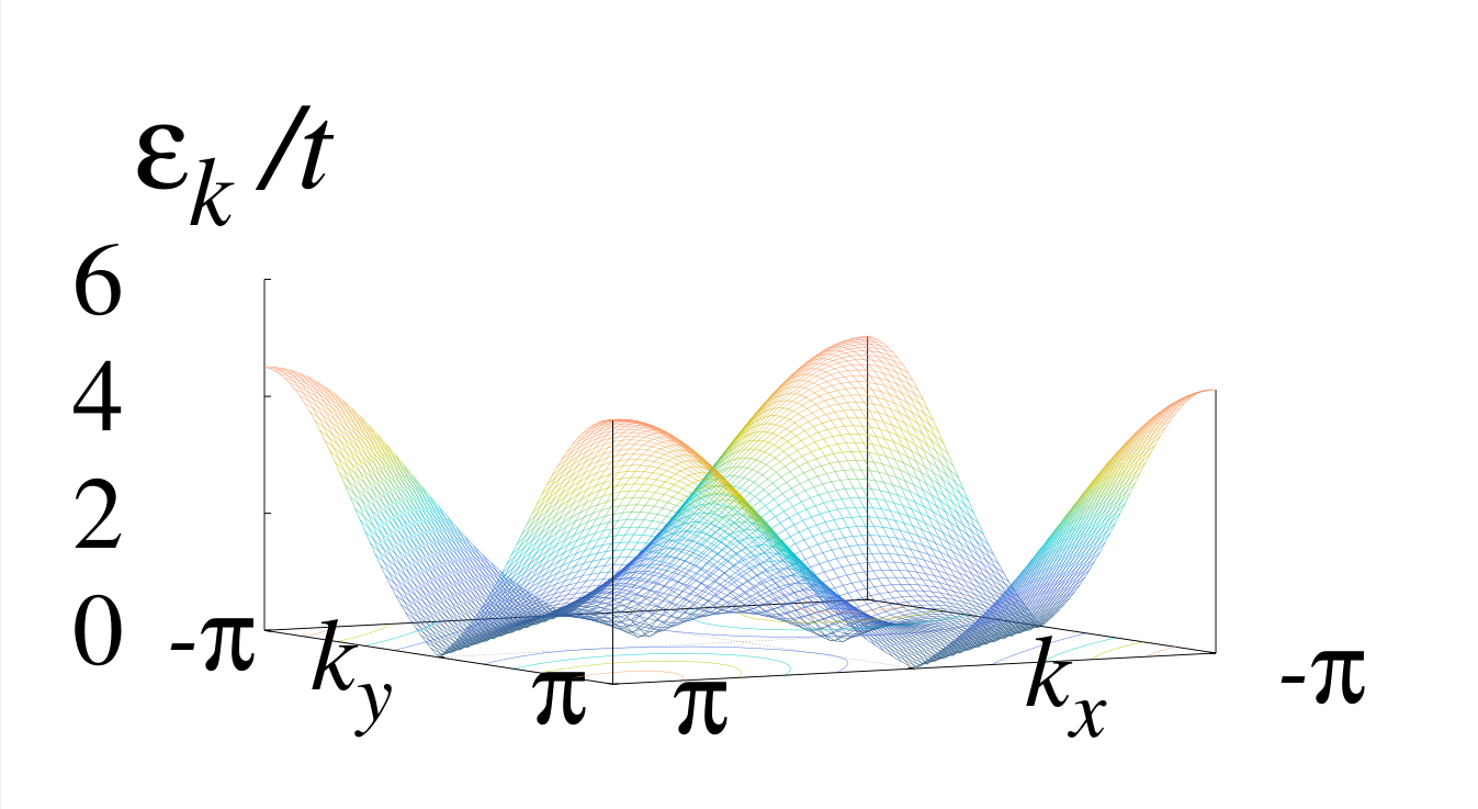
(d) $\mu=1.25t$

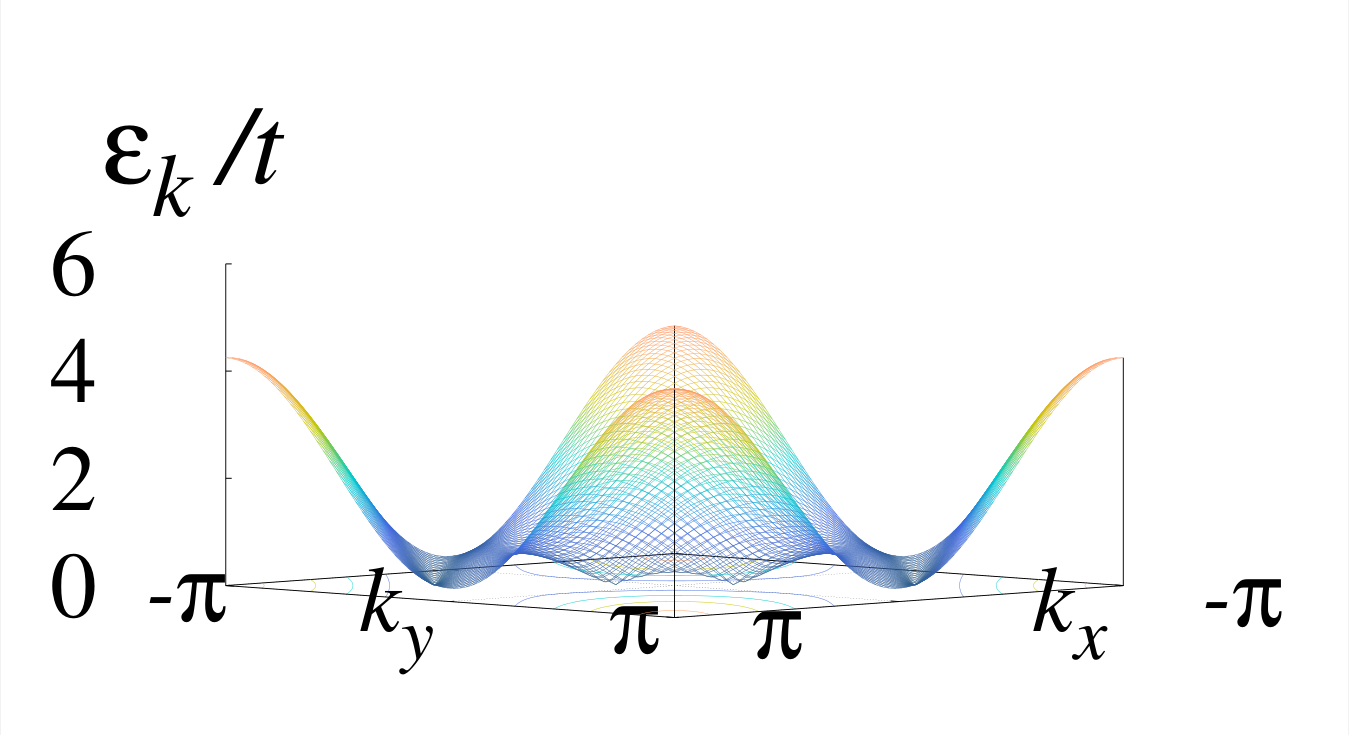
(e) $\mu=t$

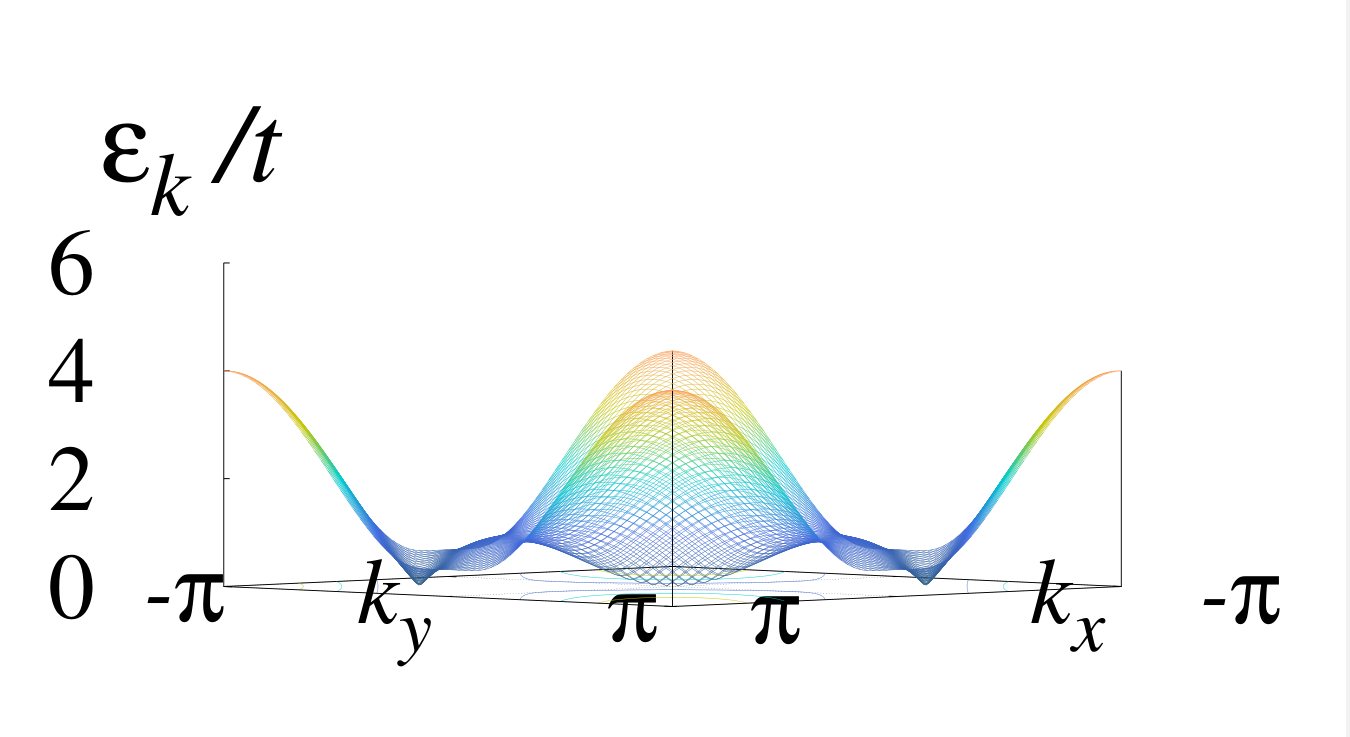
(f) $\mu=0.75t$

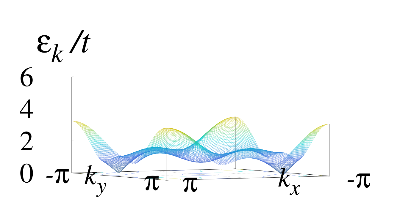
(g) $\mu=0$

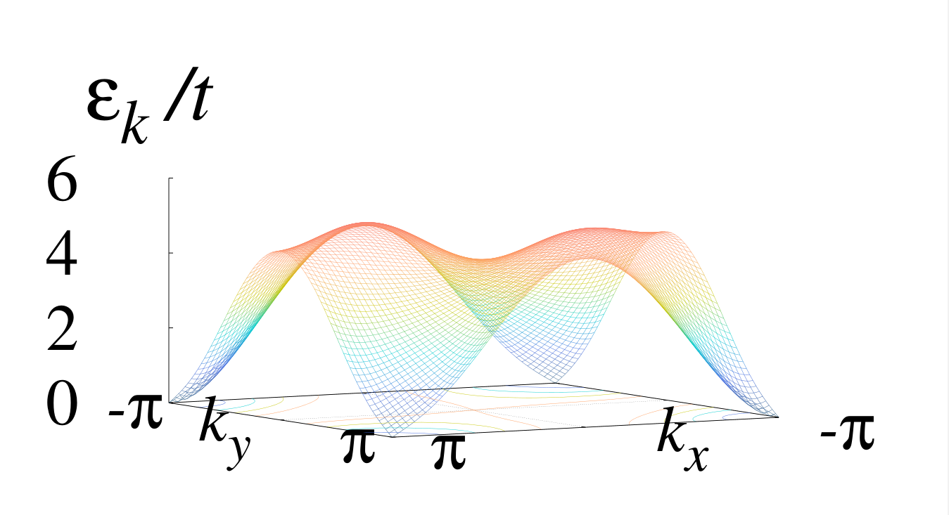
(h) $\mu=-3.25t$

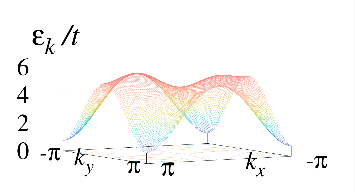
(i) $\mu=-4t$

Figure 3: Energy dispersions of the modified square-lattice Kitaev model for several values of chemical potential $\mu$ with $t^{\prime}=-1.25t$ and $\Delta=t$. The energy dispersions correspond to the filled circles on the line $t^{\prime}=-1.25t$ in Fig. 1.

The evolution of the energy dispersions with the chemical potential $\mu$ can be understood in terms of how two quasiparticle bands overlap each other. In Fig. 2 we plot the energy dispersions as $\mu$ decreases for $t^{\prime}=-0.25t$, which illustrates well the general behavior of the energy dispersions for $-\frac{1}{2}t<t^{\prime}<0$. For $\mu>t+t^{\prime}$ the two quasiparticle bands are separated by a full gap (Fig. 2(a)) and they touch each other at one gapless point $(k_{x},k_{y})=(0,0)$ when $\mu=t+t^{\prime}$ (Fig. 2(b)). Further decrease of $\mu$ forces the gapless point to split into a pair of gapless points (Fig. 2(c)), which are located on the line $k_{y}=-k_{x}$ since the pairing terms in the Hamiltonian impose the condition for zero energy. The existence of the pair is robust against the change of the chemical potential $\mu$ in that phase, implying their topological origin. Such a pair persists until they merge into a single point at $(k_{x},k_{y})=(\pi,-\pi)$ (Fig. 3(f)). It is of interest to note that a nodal line $k_{y}=k_{x}+\pi$ shows up at $\mu=-t^{\prime}$ (Fig. 3(d)) while the two gapless points approach the merging point $(\pi,-\pi)$. The band gap reopens for $\mu<-2t+t^{\prime}$.

For $t^{\prime}<-\frac{1}{2}t$, we can observe qualitatively different behavior of the energy dispersions, which are demonstrated in Fig. 3 in the case of $t^{\prime}=-1.25t$. When $t^{\prime}<-\frac{1}{2}t$, $\epsilon_{\bm{k}}$ has two minima before the two band touch each other (Fig. 3(a)), which is different from the former case. When the band gap closes at these points, two gapless points are formed (Fig. 3(b)). Each gapless point splits into two gapless points with further reduction of the chemical potential and they move away from each other along $k_{y}=-k_{x}$ (Fig. 3(c)). At $\mu=-t^{\prime}$ a nodal line $k_{y}=k_{x}+\pi$ also appears as in the case of $-\frac{1}{2}t<t^{\prime}<0$ while the inner pair of gapless points still survive (Fig. 3(d)). The inner pair merges at $(k_{x},k_{y})=(0,0)$ when $\mu=2t+t^{\prime}$ and only one pair of gapless points remains in the system (Fig. 3(f)). Finally the outer pair merges at $(k_{x},k_{y})=(\pi,-\pi)$ when $\mu=-2t-t^{\prime}$ (Fig. 3(h)) and a finite gap reopens for $\mu<-2t-t^{\prime}$ (Fig. 3(i)).

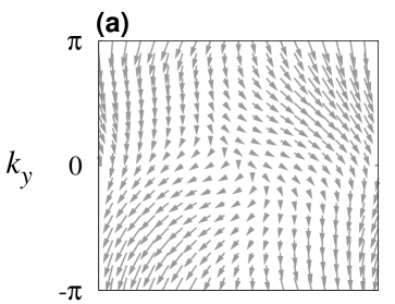
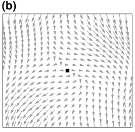
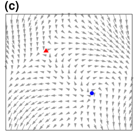
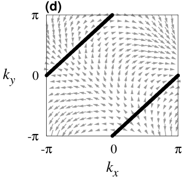
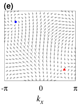
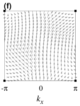
Figure 4: The vector fields $\bm{B}(\bm{k})$ of the modified square-lattice Kitaev model with $t^{\prime}=-0.25t$ and $\Delta=t$ for $\mu=$ (a) $2t$, (b) $1.75t$, (c) $t$, (d) $0.25t$, (e) $-t$, and (f) $-2.25t$, which correspond to the empty circles on the line $t^{\prime}=-0.25t$ in Fig. 1. The horizontal and vertical components of the arrows at momentum $\bm{k}$ correspond to $B_{1}(\bm{k})$ and $B_{2}(\bm{k})$, respectively. Red triangles, blue circles and black squares represent the gapless points of a winding number -1, 1, and 0, respectively.

II.4 Topological invariants of gapless points

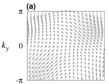
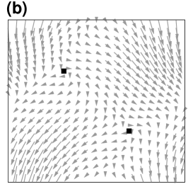
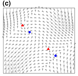
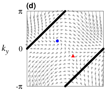
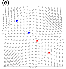
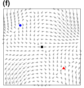
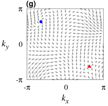
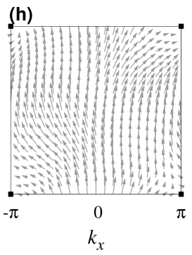
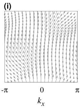
Figure 5: The vector fields $\bm{B}(\bm{k})$ of the modified square-lattice Kitaev model with $t^{\prime}=-1.25t$ and $\Delta=t$ for $\mu=$ (a) $2t$, (b) $1.65t$, (c) $1.45t$, (d) $1.25t$, (e) $t$, (f) $0.75t$, (g) $0$, (h) $-3.25t$, and (i) $-4t$, which correspond to the filled circles on the line $t^{\prime}=-1.25t$ in Fig. 1. The gapless points are marked by the same symbols as in Fig. 4.

We next examine the topological characters of individual gapless points and express the Hamiltonian matrix $h_{\bm{k}}$

$$h_{\bm{k}}=\sum_{i=1}^{2}B_{i}(\bm{k})\sigma_{i}$$ (18)

in terms of the vector field $\bm{B}(\bm{k})=(B_{1},\,B_{2})$

$$B_{1}(\bm{k}) =\Delta\left(\sin{k_{x}}+\sin{k_{y}}\right),$$

$$B_{2}(\bm{k}) =-\mu+t\left(\cos{k_{x}}+\cos{k_{y}}\right)+t^{\prime}\cos(k_{x}-k_{y}),$$ (19)

and Pauli matrices

$$\sigma_{1}=\left(\begin{matrix}0&-i\\ i&0\end{matrix}\right),\quad\quad\sigma_{2}=\left(\begin{matrix}1&0\\ 0&-1\end{matrix}\right).$$ (20)

The gapless points exist in the form of vortices (see Figs. 4 and 5). The winding number $\omega$ of each gapless point can be calculated conveniently by the expansion around the vortex center $\bm{k}_{0}$, where $\bm{k}_{0}$ is the location of the topological defect. Around the vortex center the vector field $\bm{B}(\bm{k})$ is expanded up to a linear order in $\bm{q}\equiv\bm{k}-\bm{k}_{0}$:

$$B_{1}(\bm{q})= \Delta(q_{x}\cos{k_{0x}}+q_{y}\cos{k_{0y}}),$$

$$B_{2}(\bm{q})= [-t\sin{k_{0x}}-t^{\prime}\sin(k_{0x}-k_{0y})]q_{x}$$

$$+[-t\sin{k_{0y}}+t^{\prime}\sin(k_{0x}-k_{0y})]q_{y}.$$ (21)

The matrix $h_{\bm{k}}$ is then given in the form

$$h_{\bm{k}}=\sum_{i,j=1}^{2}a_{ij}q_{i}\sigma_{j}$$ (22)

with $(q_{1},q_{2})\equiv(q_{x},q_{y})$, leading to the winding number $\omega$ of the individual topological gapless point

$$\omega = \textrm{sgn}[\textrm{det}(\bm{a})]$$

$$= \textrm{sgn}[\Delta\sin(k_{0x}-k_{0y})\left\{t+t^{\prime}(\cos{k_{0x}}+\cos{k_{0y}})\right\}].$$

We first consider the case of $-\frac{1}{2}t<t^{\prime}<0$. In Fig. 4 we plot the vector fields $\bm{B}(\bm{k})$ in the modified square-lattice Kitaev model with $t^{\prime}=-0.25t$ for several values of chemical potential $\mu$. In the system with $\mu=t+t^{\prime}$ the band gap closes, yielding a gapless point of zero winding number at $\bm{k}=(0,0)$ (see Fig. 4(b)). When the chemical potential becomes lower than this value, the gapless point splits into two Weyl-type gapless points with linear energy dispersion, one with the winding number -1 and the other with 1, while total winding number is conserved (Fig. 4(c)). The winding number of each Weyl point is not changed by the continuous change of the chemical potential $\mu$. At $\mu=-t^{\prime}$, a nodal line appear at $k_{y}=k_{x}+\pi$, making significant changes in the configuration of the vector field $\bm{B}(\bm{k})$ (Fig. 3(d)). For the chemical potential below $-t^{\prime}$, the winding numbers of the gapless points are interchanged (Fig. 3(e)). The two topological defects which have opposite winding numbers merge into one with zero winding number at ($\pi,-\pi$) for $\mu=-2t+t^{\prime}$ (Fig. 4(f)). Below this chemical potential the systems exhibits no gapless points with a finite band gap.

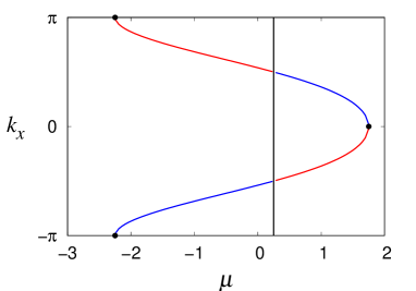
(a)

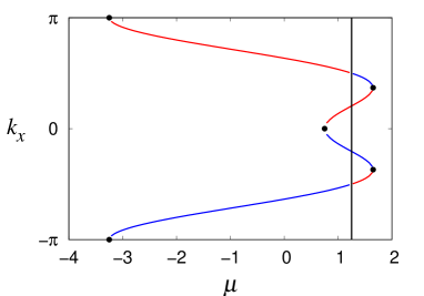
(b)

Figure 6: The $x$-component of momentum, $k_{x}$, of the topological defects as a function of the chemical potential $\mu$ for (a) $t^{\prime}=-0.25t$ and (b) $t^{\prime}=-1.25t$. Topological defects of winding number $-1/0/1$ are marked by red/black/blue lines.

The general features of the vector field $\bm{B}(\bm{k})$ for $t^{\prime}<-\frac{1}{2}t$ are demonstrated well in Fig. 5, which shows the vector fields $\bm{B}(\bm{k})$ for $t^{\prime}=-1.25t$. In contrast to the case with $-\frac{1}{2}t<t^{\prime}<0$, the system exhibits two gapless points when the band gap closes; the winding numbers of both gapless points are zero (Fig. 5(b)). Each topological defect splits into two gapless points, resulting in two pairs of Weyl points whose winding numbers are opposite to each other (Fig. 5(c)). As in the case with $-\frac{1}{2}t<t^{\prime}<0$, a nodal line, $k_{y}=k_{x}+\pi$, shows up for $\mu=-t^{\prime}$, which interchanges their winding numbers of an outer pair of Weyl points only (Fig. 5(d)). The inner pair of Weyl points approach each other (see Fig. 5(e)) and merge at $\bm{k}=(0,0)$ (Fig. 5(f)). The remaining pair of Weyl points also merge into a trivial gapless point at $(\pi,-\pi)$ (Fig. 5(h)) at a lower chemical potential, below which the system lies in a trivial gapful phase without any topological gapless point (Fig. 5(i)).

Figure 6 displays the variation of the momentum of gapless points and their winding numbers with the chemical potential $\mu$ for $t^{\prime}=-0.25t$ and $t^{\prime}=-1.25t$. It is sufficient to plot the $x$-component only of the momentum of gapless points for the accurate description of the gapless-point position since all the isolated topological defects with winding number $\pm 1$ are on the line $k_{y}=-k_{x}$ and a nodal line of winding number zero is given by $k_{y}=k_{x}+\pi$ in the whole range of $k_{x}$. For $-\frac{1}{2}t<t^{\prime}<0$, as shown in Fig. 6(a), a gapless point of winding number zero is formed at $\bm{k}=(0,0)$ for $\mu=2t+t^{\prime}$. As the chemical potential is reduced , it evolves to two separate topological Weyl points; the $x$-component momentum of the one with winding number $+1$ increase while the other with winding number $-1$ moves towards $(-\pi,\pi)$. The nodal line , which shows up for $\mu=-t^{\prime}$, flips the winding number of both Weyl points. They approach $(-\pi,\pi)$ monotonically from the opposite directions and transforms to one gapless point with zero winding number, which disappears for $\mu<-2t+t^{\prime}$.

For $t^{\prime}<-\frac{1}{2}t$, on the other hand, the system exhibits two trivial gapless points for $\mu=-t^{2}/(2t^{\prime})-t^{\prime}$. From each trivial gapless point two topological Weyl points are produced; the inner pair of Weyl points, which are closer to the origin, approach each other, and merge at the origin for $\mu=2t+t^{\prime}$. The outer pair moves away from the origin and finally meets to form a trivial gapless point at $(-\pi,\pi)$ for $\mu=-2t+t^{\prime}$. Winding numbers are affected by the nodal line, which is formed for $\mu=-t^{\prime}$, only for the outer pair of Weyl points.

II.5 Majorana flat band edge modes in ribbon geometry

In this section, we consider the modified square-lattice Kitaev model in the ribbon geometry to examine the topological edge states which is characteristics of topological bulk states in the system. It turns out that the accompanying edge states are Majorana flat bands formed at the edges.

Figure 7: Energy dispersions of the modified square-lattice Kitaev model in the ribbon of width $N_{x}=80$ for $t^{\prime}=-0.25t$, $\Delta=t$ and $\mu=$ (a) $2t$; (b) $1.75t$; (c) $t$; (d) $0.25t$; (e) $-t$; (f) $-2.25t$. The energy dispersions displayed in this figure correspond to the empty circles at $t^{\prime}=-0.25t$ in Fig. 1.

we obtain the Hamiltonian of a block diagonal form

For this purpose, it is convenient to define two Majorana operators given by

$$a_{\bm{r}} \equiv c^{\dagger}_{\bm{r}}+c_{\bm{r}},$$

$$b_{\bm{r}} \equiv-i\left(c^{\dagger}_{\bm{r}}-c_{\bm{r}}\right),$$ (24)

which satisfy the anticommutation relations

$$\{a_{\bm{r}},a_{\bm{r}^{\prime}}\} =2\delta_{\bm{r},\bm{r}^{\prime}},$$

$$\{b_{\bm{r}},b_{\bm{r}^{\prime}}\} =2\delta_{\bm{r},\bm{r}^{\prime}},$$

$$\{a_{\bm{r}},b_{\bm{r}^{\prime}}\} =0.$$ (25)

Inserting Eq. (24) into Eq. (1), we obtain the Hamiltonian of the form

$$H=\frac{i}{4}\sum_{\bm{r}} \bigg{[}\left(t+\Delta\right)\sum_{\bm{a}}a_{\bm{r}}b_{\bm{r}+\bm{a}}+\left(t-\Delta\right)\sum_{\bm{a}}a_{\bm{r}+\bm{a}}b_{\bm{r}}$$

$$+\,t^{\prime}a_{\bm{r}}b_{\bm{r}+\bm{b}^{\prime}}+\,t^{\prime}a_{\bm{r}+\bm{b}^{\prime}}b_{\bm{r}}-2\mu a_{\bm{r}}b_{\bm{r}}-h.c.\bigg{]}.$$ (26)

We employ open boundary conditions in the $x$ direction and periodic boundary conditions in the $y$ direction. The $N_{x}\times N_{y}$ lattice sites in the ribbon can be denoted by $\bm{r}=ma\hat{\bm{i}}+na\hat{\bm{j}}(m=1,2,\cdots,N_{x},n=1,2,\cdots N_{y})$. Then the Hamiltonian in the ribbon geometry can be written

$$H_{N_{x}}=\frac{i}{4}\sum^{N_{x}}_{m=1}\sum^{N_{y}}_{n=1} \big{[}\left(t-\Delta\right)\left(a_{m,n+1}b_{m,n}+a_{m+1,n}b_{m,n}\right)$$

$$+\left(t+\Delta\right)\left(a_{m,n}b_{m,n+1}+a_{m,n}b_{m+1,n}\right)$$

$$+t^{\prime}(a_{m,n}b_{m+1,n-1}+a_{m+1,n-1}b_{m,n})$$

$$-2\mu a_{m,n}b_{m,n}-h.c.\big{]}$$ (27)

with the assumptions

$$a_{m,N_{y}{+}1} =a_{m,1},$$

$$b_{m,N_{y}{+}1} =b_{m,1},$$

$$a_{N_{x}{+}1,n} =b_{N_{x}{+}1,n}=0.$$ (28)

Figure 8: Energy dispersions of the modified square-lattice Kitaev model in the ribbon of width $N_{x}=80$ for $t^{\prime}=-0.25t$, $\Delta=t$, and $\mu=$ (a) $2t$; (b) $1.65t$; (c) $1.45t$; (d) $1.25t$; (e) $t$; (f) $0.75t$; (g) $0$; (h) $-3.25t$; (i) $-4t$. The energy dispersions displayed in this figure correspond to the filled circles at $t^{\prime}=-1.25t$ in Fig. 1.

Taking Fourier transformation of Majorana operators in the $y$ direction

$$a_{m,n} = \displaystyle\frac{1}{\sqrt{N_{y}}}\sum_{k_{y}}e^{ik_{y}n}\alpha_{m,k_{y}},$$

$$b_{m,n} = \displaystyle\frac{1}{\sqrt{N_{y}}}\sum_{k_{y}}e^{ik_{y}n}\beta_{m,k_{y}},$$ (29)

$$H_{N_{x}}=\sum_{k_{y}} H^{k_{y}}_{N_{x}}$$

with

$$H^{k_{y}}_{N_{x}}=\sum^{N_{x}-1}_{m=1}\big{[} \eta\,\alpha_{m,k_{y}}i\beta_{m,-k_{y}}+\delta_{1D}\,\alpha_{m+1,k_{y}}i\beta_{m,-k_{y}}$$

$$+\delta_{2D}\,\alpha_{m,k_{y}}i\beta_{m+1,-k_{y}}\big{]}$$

$$+\eta\,\alpha_{N_{x},k_{y}}i\beta_{N_{x},-k_{y}}+h.c.,$$ (30)

where

$$\eta\equiv\frac{1}{4}[\left(t-\Delta\right)e^{ik_{y}}+\left(t+\Delta\right)e^{-ik_{y}}-2\mu],$$

$$\delta_{1D}\equiv\frac{1}{4}\left(t-\Delta+t^{\prime}e^{-ik_{y}}\right),$$

$$\delta_{2D}\equiv\frac{1}{4}\left(t+\Delta+t^{\prime}e^{ik_{y}}\right).$$ (31)

We calculate the eigenvalues of $H^{k_{y}}_{N_{x}}$ numerically to obtain the energy spectra for $k_{y}$, which yields the energy dispersions in the ribbon. We plot the energy dispersions of two typical cases, $t^{\prime}=-0.25t$ and $t^{\prime}=-1.25t$, in Figs. 7 and 8, respectively.

For $-\frac{1}{2}t<t^{\prime}<0$, we find that Majorana zero modes show up when a gapless point splits into two Weyl points. In Fig. 7(c), we observe Majorana zero modes in the interval, the end points of which are the projections of two bulk Weyl points on the $k_{y}$ axis. At $\mu=-t^{\prime}$, where a nodal line exists in the bulk, the ribbon becomes metallic. For lower chemical potentials, the ribbon still exhibits a Majorana flat band, whose interval contains $k_{y}=\pi$ instead of $k_{y}=0$. As the chemical potential decreases further, the interval of Majorana band shrinks gradually, and the flat band disappears when a pair of Weyl points merge into a point (Fig. 7(f)).

For $t^{\prime}<-\frac{1}{2}t$, the remarkable feature is that two Majorana flat bands exist in the energy dispersions (Fig. 8(c)); this has its origin in the fact that the system has four Weyl points which are generated from two separate trivial gapless points in the bulk. The ribbon also exhibits metallic dispersions at $\mu=-t^{\prime}$ (Fig. 8(d)), and the reduction of the chemical potential below this value changes the region of zero-energy edge modes. One interval contains $k_{y}=0$ and the other $k_{y}=\pi$ (Fig. 8(e)). The one with $k_{y}=0$, which connects the inner pair of Weyl points, first disappears (see Fig. 8(f)), and for $\mu=-2t+t^{\prime}$ the other finally disappears (see Fig. 8(h)).

The analytical approach for the existence of Majorana zero-energy edge modes also sheds some insights on our understanding. We express $H^{k_{y}}_{N_{x}}$ in terms of a vector $V_{k_{y}}\equiv\left(\alpha_{1,k_{y}}\;\,\beta_{1,k_{y}}\;\,\alpha_{2,k_{y}}\;\,\beta_{2,k_{y}}\;\cdots\;\alpha_{N_{x},k_{y}}\;\,\beta_{N_{x},k_{y}}\right)$, leading to

$$\begin{matrix}H^{k_{y}}_{N_{x}}=V_{k_{y}}\,h^{k_{y}}_{N_{x}}\,V^{\dagger}_{k_{y}}.\end{matrix}$$ (32)

When we impose that the eigenenergy be exactly zero, we can find that the corresponding eigenstates of $h^{k_{y}}_{N_{x}}$ which satisfy the open boundary conditions in the $x$ direction can exist only in two ways; for $|p_{\pm}|<1$

$$\gamma_{k_{y}}^{(1)} = A_{1}\sum_{m=1}^{N_{x}}\left[(p_{+})^{m}-(p_{-})^{m}\right]\beta_{m,k_{y}},$$ (33)

$$\gamma_{k_{y}}^{(2)} = A_{2}\sum_{m=1}^{N_{x}}\left[({p_{-}}^{*})^{N_{x}+1-m}-({p_{+}}^{*})^{N_{x}+1-m}\right]\alpha_{m,k_{y}}$$

and for $|p_{\pm}|>1$

$$\gamma_{k_{y}}^{(1)} = A_{3}\sum_{m=1}^{N_{x}}\left[({p_{-}}^{*})^{-m}-({p_{+}}^{*})^{-m}\right]\alpha_{m,k_{y}}.$$ (35)

$$\gamma_{k_{y}}^{(2)} = A_{4}\sum_{m=1}^{N_{x}}\left[(p_{+})^{m-N_{x}-1}-(p_{-})^{m-N_{x}-1}\right]\beta_{m,k_{y}},$$

where

$$p_{\pm}\equiv\frac{-\eta\pm\sqrt{\eta^{2}-4\delta_{1D}\delta_{2D}}}{2\delta_{2D}}$$ (37)

and $A_{i}$’s are normalized constants. Majorana zero-energy eigenstates $\gamma_{k_{y}}^{(1)}$ and $\gamma_{k_{y}}^{(2)}$ are localized around $m=1$ and $m=N_{x}$, respectively, and satisfy the boundary condition at the opposite edge only in the limit of infinite width of the ribbon.

The necessary and sufficient condition for the existence of Majorana zero-energy modes is given by

$$\left(|p_{+}|-1\right)\left(|p_{-}|-1\right)>0.$$ (38)

Equation (38) combined with Eq. (37) leads to an inequality for $k_{y}$

$$\left(\mu+t^{\prime}\right)\left(-2t^{\prime}\cos^{2}{k_{y}}-2t\cos{k_{y}}+\mu+t^{\prime}\right)<0.$$ (39)

We verified that the intervals of Majorana flat bands that the inequality in Eq. (39) produces are in complete agreement with the numerical results in Figs. 7 and 8. Particularly, the abrupt inversion of flat bands which occurs at $\mu=-t^{\prime}$ can be attributed to the prefactor $\mu+t^{\prime}$ in Eq. (39).

It is also remarkable that Eqs. (33)-(LABEL:eq_Kitaev_zeromodes2) predict which type of Majorana fermions exists at the edges. According to Eqs. (33)-(LABEL:eq_Kitaev_zeromodes2), in the region with $|p_{\pm}|<1$ Majorana fermions of a $\beta$ type exist at the edges of $m=1$ and $\alpha$-type Majorana fermions around $m=N_{x}$. For $|p_{\pm}|>1$, on the other hand, $\alpha$-type ones at $m=1$ while $\beta$-type ones at $m=N_{x}$. We observe that these predictions agree well with numerical results presented above. In the energy dispersion of Fig. 8(c), the intervals of both flat bands satisfy $|p_{\pm}|<1$. Numerically computed eigenstates demonstrate that these bands are degenerate with two eigenstates; one with only $\alpha$-type components occupied is localized around $m=N_{x}$ and the other with only $\beta$-type components occupied is localized around $m=1$. We can find different cases in Fig. 8(e), The inner flat bands containing $k_{y}=0$ satisfy $|p_{\pm}|<1$ and belong to the same class of the flat bands described above. The flat band around $k_{y}=\pi$ with $|p_{\pm}|>1$, on the other hand, turns out to produce $\alpha$-type Majorana fermions around $m=1$ and $\beta$-type ones around $m=N_{x}$. and this reproduces well the prediction by the above analytical approach.

III Summary

In this paper, we have considered the modified square-lattice Kitaev model, paying attention to the effects of additional next-nearest-neighbor hopping on topological gapless phases and Majorana zero-energy edge modes. In addition to the topological gapless phase with two gapless points, which the original model exhibits in the presence of nearest neighbor hopping only, we have discovered newly emergent topological phases with four gapless points in the bulk.

The variation of the positions and the topological characters of the gapless points has been explored in detail as chemical potential changes in the bulk energy spectra. We have also investigated the evolution of Majorana zero modes in the energy dispersions of the ribbon geometry.

Particularly, we have derived the analytical expression which determines the location of the Majorana flat bands from the constraints on the boundary conditions of zero-energy edge modes; this is in complete agreement with all the numerical results. A detailed analytical analysis on the eigenstates corresponding to Majorana zero-energy modes has provided deeper understanding on the presence of two types of Majorana fermion which has its origin in topological features of the system.