Multiplicative noise removal based on a variable-order fractional diffusion model

Abstract.

In this paper, we propose a new model using a variable-order fractional $1$-Laplacian diffusion equation for multiplicative noise removal. The existence and uniqueness of the weak solution are proven. To overcome the difficulties in the approximation process, we place particular emphasis on studying the density properties of the variable-order fractional Sobolev spaces. Numerical experiments demonstrate that our model exhibits favorable performance across the entire image.

1. Introduction

Multiplicative noise affects images in many fields, including synthetic aperture radar (SAR), ultrasonic imaging, and optical coherence tomography. The observed image $f$ is the pointwise product of the original image $u$ and noise $\eta$. Recovering the original image $u$ from degraded input $f$ is the main task in multiplicative noise removal, which constitutes a critical challenge in the field of image denoising. In the past three decades, a variety of methods based on reaction-diffusion equations have been proposed for image denoising. The classical diffusion equations for a density function $u$ can be traced back to the fundamental conservation law $u_{t}+\operatorname{div}(\vec{J})=0$, where $\vec{J}$ is the diffusion flux defined by Fick’s first law $\vec{J}=-c\nabla u$. Assuming that the diffusion coefficient $a$ depends on the distribution in a manner expressed as a function $c=c(u)$, the equation is transformed to a nonlinear diffusion equation

$$\frac{\partial u}{\partial t}=\operatorname{div}\left(c(u)\nabla u\right),$$ (1.1)

taking $c(u)=|\nabla u|^{p-2}$ ($1\leqslant p<\infty$), then (1.1) becomes the well-known $p$-Laplacian equation

$$\frac{\partial u}{\partial t}=\operatorname{div}\left(|\nabla u|^{p-2}\nabla u\right),$$ (1.2)

which has been extensively investigated for image processing [1]. If $p=2$, this is the heat equation, which is equivalent to using a Gaussian filter for image denoising, leading to an overly smooth restoration of the image. If $p=1$, (1.2) is the total variation (TV) flow, which comes from the gradient decent scheme of the ROF model [2]. Other types of nonlinear diffusion flows, in addition to the TV flow, have also been shown to effectively remove additive noise, see [3, 4, 5, 6, 7].

To perform the task of the multiplicative noise removal, inspired by the ROF model, Aubert and Aujol proposed the following (AA) variational model [8] using maximum a posteriori estimation (MAP),

$$E_{AA}(u)=\int_{\Omega}|Du|+\int_{\Omega}\left(\log u+\frac{f}{u}\right)dx,$$ (1.3)

and proved the existence and the local uniqueness of (1.3). The associated evolution problem of (1.3) is

$$\vspace{0.2em}\frac{\partial u}{\partial t}=\operatorname{div}\left(\frac{\nabla u}{|\nabla u|}\right)+\lambda\frac{f-u}{u^{2}},\, \textrm{~{}~{}~{}in~{}~{}}(0,T)\times\Omega,$$ (1.4a)

$$\left\langle\nabla u,\vec{n}\right\rangle=0, \textrm{~{}~{}~{}on~{}~{}}(0,T)\times\partial\Omega,$$ (1.4b)

$$u(0,x)=f, \textrm{~{}~{}~{}on~{}~{}}\Omega,$$ (1.4c)

with (1.4a) being interpretable as a source term added to the TV flow. For other important variational models for multiplicative noise removal, see [9, 10, 11, 12]. The authors of [13] proposed a framework for multiplicative noise removal based on nonlinear diffusion equations. They have found that incorporating a source term derived from the variational problem into the diffusion equation may impede noise removal. As a result, it is recommended to select the source term as $0$ and accomplish the task of removing multiplicative noise by designing the diffusion coefficient in terms of $u$. For more diffusion-based models for multiplicative noise removal without a source term, we refer to [14, 15, 16, 17]. By appropriately selecting the diffusion coefficient, both the edge and homogeneous regions can be restored during the process of image denoising. However, the previously mentioned models solely rely on local image information, thus fall short in preserving the texture and repetitive structures in images.

To effectively handle textures and repetitive structures in algorithms based on PDEs, it is proposed to utilize nonlocal operators for defining novel types of flows and functionals in image processing and related fields [18]. Let $\Omega\subset\mathbb{R}^{N}$, $x,y\in\Omega$, $u(x)$ be a real function $u:\Omega\to\mathbb{R}$, $v(x,y)$ be a vector field $\vec{v}:\Omega\times\Omega\to\mathbb{R}$, $w(x,y)\geqslant 0$ is a symmetric weight function. The nonlocal gradient $\nabla_{\mathrm{NL}}u:\Omega\times\Omega\to\mathbb{R}$ is defined as

$$(\nabla_{\mathrm{NL}}u)(x,y)\coloneqq(u(y)-u(x))\sqrt{w(x,y)},$$

and the nonlocal divergence $\operatorname{div}_{\mathrm{NL}}\vec{v}:\Omega\to\mathbb{R}$ is defined as

$$(\operatorname{div}_{\mathrm{NL}}\vec{v})(x)\coloneqq\int_{\Omega}(v(x,y)-v(y,x))\sqrt{w(x,y)}dy,$$

Similar to the usual nonlinear diffusion equation, let $c(u):\Omega\times\Omega\to\mathbb{R}$ be a symmetric function, then a nonlinear nonlocal diffusion operator can be defined as

$$\mathcal{N}u(x)=\frac{1}{2}\operatorname{div}_{\mathrm{NL}}\left(c(u)\nabla_{\mathrm{NL}}u\right)(x)=\int_{\Omega}(c(u)(x,y))(u(y)-u(x))w(x,y)dy,$$

then a nonlinear nonlocal diffusion process can be written as

$$\vspace{0.2em}\frac{\partial u}{\partial t}=\mathcal{N}u,\,\textrm{~{}~{}~{}~{}in~{}~{}}(0,T)\times\Omega,$$ (1.5a)

$$u(0,x)=f,\textrm{~{}~{}~{}on~{}~{}}\Omega.$$ (1.5b)

In the context of image processing, the authors of [19] suggested using the weight function $w(x,y)$ to measure nonlocal similarity between two patches, with further applications documented in [20, 21, 18]. Various nonlocal diffusion models can be obtained by appropriately selecting $c(u)$ and $w(x,y)$. Let $J:\mathbb{R}^{N}\to\mathbb{R}^{N}$ be a nonnegative continuous radial function with compact support, $J(0)>0$, and $\int_{\mathbb{R}^{N}}J(z)dz=1$, for $c(u)(x,y)=|u(y)-u(x)|^{p-2}$, $w(x,y)=J(x-y)$, (1.5a) becomes a nonlocal $p$-Laplacian evolution equation

$$\frac{\partial u}{\partial t}=\int_{\Omega}J(x-y)\left|u(t,y)-u(t,x)\right|^{p-2}\left(u(t,y)-u(t,x)\right)dy,$$ (1.6)

which has been studied in [22, 23]. If the kernel $J$ is appropriately rescaled, the solutions of (1.6) converges strongly in $L^{p}$ to the solution of (1.2) with Neumann condition. For $c(u)(x,y)=|u(y)-u(x)|^{p-2}$, $w(x,y)=|x-y|^{-(N+sp)}$, (1.5a) becomes a fractional $p$-Laplacian evolution equation

$$\frac{\partial u}{\partial t}=\int_{\Omega}\frac{1}{|x-y|^{N+sp}}\left|u(t,y)-u(t,x)\right|^{p-2}\left(u(t,y)-u(t,x)\right)dy,$$ (1.7)

which has been studied in [24]. For $s<1$ close to $1$, the solution of (1.7) converges strongly in $L^{p}$ to the solution of with Neumann condition when $s\to 1^{-}$. If $p=2$, this is the well-known fractional Laplacian evolution equation. The fractional Laplacian $(-\Delta)^{s}$ arises in a number of applications such as anomalous diffusion, Lévy process, Gaussian random fields, quantum mechanics, see [25, 26, 27, 28] and the references therein. For applications of the fractional Laplacian in image denoising problems, see [29, 30]. The authors of [31] proposed the use of the fractional $1$-Laplacian in reaction-diffusion systems and applied it for additive noise removal. Combining the fractional 1-Laplacian and AA model, the following model [32]

$$\left\{\begin{array}[]{ll}\displaystyle\vspace{0.2em}\frac{\partial u}{\partial t}=\int_{\Omega}\frac{k(x,y)}{|x-y|^{N+s}}\dfrac{u(t,y)-u(t,x)}{\left|u(t,y)-u(t,x)\right|}dy+\lambda\dfrac{f-u}{u^{2}},&\textrm{in~{}~{}}(0,T)\times\Omega,\\ u(0,x)=f,&\textrm{on~{}~{}}\Omega,\end{array}\right.$$

was proposed to remove multiplicative noise. This model is referred to as the F1P-AA model in this article. The function $k(x,y)$ in the F1P-AA model can be appropriately selected to enhance the model’s self-adaptability. The previously mentioned nonlocal methods perform well in removing noise in homogeneous regions and preserving textures, however, they also have two opposite drawbacks: causing over-smoothness in low-contrast regions and leaving residual noise around edges [33].

In practical images, there are often both homogeneous regions and edges, as well as textures and repetitive structures. In order to make nonlocal methods perform well across the entire image, there are currently two approaches. The first approach is to combine local and nonlocal methods, as shown in [33, 34, 35, 36]. The other approach is letting $s$ be spatially dependent in the fractional-order operator. A variational model based on variable-order $x\mapsto s(x)$ was proposed in [37], which can be viewed as a preliminary attempt to apply variable-order fractional Laplacian for image denoising. The established variational model is built on the basis of the Stinga-Torrea extension, instead of directly defining $(-\Delta)^{s(x)}$, because there is no clear way to define $(-\Delta)^{s(x)}$, actually. The well-defined variable-order fractional Laplacian $(-\Delta)^{s(\cdot,\cdot)}$ (see [38]) and the variable-order fractional $p$-Laplacian $(-\Delta)_{p}^{s(\cdot,\cdot)}$ (see [39]) have not been applied to image processing yet, and there are rare theoretical results on their evolution problems.

Inspired by the models mentioned above, we propose a new variable-order fractional $1$-Laplacian diffusion model for multiplicative noise removal:

$$\left\{\begin{array}[]{ll}\displaystyle\vspace{0.2em}\frac{\partial u}{\partial t}=\int_{\Omega}\frac{k(x,y)}{|x-y|^{N+s(x,y)}}\dfrac{u(t,y)-u(t,x)}{\left|u(t,y)-u(t,x)\right|}dy,&\textrm{in~{}~{}}(0,T)\times\Omega,\\ u(0,x)=f,&\textrm{on~{}~{}}\Omega,\end{array}\right.$$ (1.8)

where $\Omega\subset\mathbb{R}^{N}$ with $N\geqslant 2$ is an open set of class $C^{0,1}$ with bounded boundary, $T>0$, $f$ is a positive measurable function, $s:\mathbb{R}^{N}\times\mathbb{R}^{N}\to(0,1)$ is some symmetric, continuous function, and $k(x,y)=k(f)(x,y)$ is some nonnegative symmetric weight function with compact support. Compared with the F1P-AA model, our model offers two unique benefits: enhanced self-adaptability through the selection of spatially dependent $s(x,y)$ and thorough denoising due to the absence of a source term. Based on the numerical experiments, it has been demonstrated that our model exhibits favorable performance across the entire image. In comparison with the F1P-AA model, our model is more effective in terms of denoising effects.

The rest of this paper is organized as follows. We state some necessary preliminaries about variable-order fractional Sobolev spaces and the main result in Section 2. In section 3, we prove more basic results of the space $W^{s(\cdot,\cdot),p}(\Omega)$, especially density properties. The existence and uniqueness of the variable-order fractional $p$-Laplacian evolution equations when $1<p<2$ is proven in Section 4. In Section 5, we prove that problem (1.8) admits a unique weak solution. Some properties of the weak solutions of (1.8) are presented in Section 6. Finally, we show some numerical experiments in Section 7 to demonstrate the effectiveness of denoising by our model.

2. Mathematical Preliminaries and main result

In this section, we state some necessary preliminaries of variable-order fractional Sobolev spaces that will be used below. We refer to [38, 39] and the references therein for some detailed proof. Henceforth, we will always assume that $\Omega$ is an open set in $\mathbb{R}^{N}$, $1\leqslant p<+\infty$, $s:\mathbb{R}^{N}\times\mathbb{R}^{N}\to(0,1)$ is a symmetric, continuous function satisfies

$$0<s^{-}=\inf_{(x,y)\in\mathbb{R}^{N}\times\mathbb{R}^{N}}s(x,y)\leqslant s(x,y)\leqslant s^{+}=\sup_{(x,y)\in\mathbb{R}^{N}\times\mathbb{R}^{N}}s(x,y)<1.$$

Denote by

$$[u]_{W^{s(\cdot,\cdot),p}(\Omega)}=\left(\int_{\Omega}\int_{\Omega}\frac{\left|u(y)-u(x)\right|^{p}}{|x-y|^{N+s(x,y)p}}dxdy\right)^{\frac{1}{p}}$$

the Gagliardo seminorm with variable order of a measurable function $u$ in $\Omega$. We consider the variable-order fractional Sobolev spaces

$$W^{s(\cdot,\cdot),p}(\Omega)=\left\{u\in L^{p}(\Omega)\ :\ [u]_{W^{s(\cdot,\cdot),p}(\Omega)}<+\infty\right\},$$

which is a Banach space with respect to the norm

$$\|u\|_{W^{s(\cdot,\cdot),p}(\Omega)}\coloneqq\|u\|_{L^{p}(\Omega)}+[u]_{W^{s(\cdot,\cdot),p}(\Omega)}.$$

Now let $\Omega$ be an open set with bounded boundary. Define the operator $T:W^{s(\cdot,\cdot),p}(\Omega)\to L^{p}(\Omega)\times L^{p}(\Omega\times\Omega)$ by

$$T(u)=\left(u(x),\frac{u(x)-u(y)}{|x-y|^{\frac{N}{p}+s(x,y)}}\right),$$

clearly $T$ is an isometry. Thus, $W^{s(\cdot,\cdot),p}(\Omega)$ is separable (see [40, Proposition 3.20]), moreover, if $p>1$, $W^{s(\cdot,\cdot),p}(\Omega)$ is reflexive (see [40, Proposition 3.25]).

In this paper, we assume that $k(x,y)\in L^{\infty}(\Omega\times\Omega)$ is symmetric and there exist constants $0<\delta_{1}<\delta_{2}$, and $C_{1}>0$, $C_{2}>0$ such that

$$C_{1}\chi_{\{|x-y|<\delta_{1}\}}\leqslant k(x,y)\leqslant C_{2}\chi_{\{|x-y|<\delta_{2}\}}$$

for all $(x,y)\in\Omega\times\Omega$. Similar to Lemma 2.2 in [32], we shall prove a lemma concerning boundedness.

Lemma 2.1.

Let $\Omega$ be an open set with bounded boundary. Let $1\leqslant p<2$. If there exists a constant $C_{0}>0$ such that

$$\int_{\Omega}|u(x)|^{2}dx+\int_{\Omega}\int_{\Omega}\frac{k(x,y)}{|x-y|^{N+s(x,y)p}}\left|u(y)-u(x)\right|^{p}dxdy\leqslant C_{0},$$

then we have $u\in L^{2}(\Omega)\cap W^{s(\cdot,\cdot),p}(\Omega)$ with

$$\int_{\Omega}|u(x)|^{2}dx+\int_{\Omega}\int_{\Omega}\frac{\left|u(y)-u(x)\right|^{p}}{|x-y|^{N+s(x,y)p}}dxdy\leqslant C(C_{1},C_{0},\delta_{1},N,|\Omega|).$$

Proof.

We only need to show that $[u]_{W^{s(\cdot,\cdot),p}(\Omega)}$ is bounded. Since $k(x,y)\geqslant 0$ and by Hölder’s inequality, we have

$$\left[u\right]_{W^{s(\cdot,\cdot),p}(\Omega)}^{p}= \int_{\Omega}\int_{\Omega}\frac{|u(x)-u(y)|^{p}}{|x-y|^{N+s(x,y)p}}dxdy$$

$$= \iint_{\{|x-y|<\delta_{1}\}}\frac{|u(x)-u(y)|^{p}}{|x-y|^{N+s(x,y)p}}dxdy+\iint_{\{|x-y|\geqslant\delta_{1}\}}\frac{|u(x)-u(y)|^{p}}{|x-y|^{N+s(x,y)p}}dxdy$$

$$\leqslant \frac{1}{C_{1}}\iint_{\{|x-y|<\delta_{1}\}}\frac{k(x,y)}{|x-y|^{N+s(x,y)p}}|u(x)-u(y)|^{p}dxdy$$

$$+\frac{1}{\min\big{\{}1,\delta_{1}^{N+2}\big{\}}}\iint_{\{|x-y|\geqslant\delta_{1}\}}|u(x)-u(y)|^{p}dxdy$$

$$\leqslant \frac{C_{0}}{C_{1}}+\frac{2^{p-1}}{\min\big{\{}1,\delta_{1}^{N+2}\big{\}}}\int_{\Omega}\int_{\Omega}\left(|u(x)|^{p}+|u(y)|^{p}\right)dxdy$$

$$\leqslant \frac{C_{0}}{C_{1}}+\frac{2^{p}}{\min\big{\{}1,\delta_{1}^{N+2}\big{\}}}\left(\int_{\Omega}|u|^{2}dx\right)^{\frac{p}{2}}|\Omega|^{2-\frac{p}{2}}$$

$$\leqslant \frac{C_{0}}{C_{1}}+\frac{4\big{(}\|u\|_{L^{2}(\Omega)}^{2}+1\big{)}\big{(}|\Omega|^{2}+1\big{)}}{\min\big{\{}1,\delta_{1}^{N+2}\big{\}}}$$

$$= C(C_{1},C_{0},\delta_{1},N,|\Omega|).$$

This concludes the proof. ∎

Remark 2.2.

From this lemma, we know that when $1\leqslant p<2$, for a sequence $\{u_{k}\}\subset W^{s(\cdot,\cdot),p}(\Omega)$, if $\{u_{k}\}$ is bounded in $L^{2}(\Omega)$ and there exists a positive constant $C$ independent of $k=1,2,\cdots$ such that

$$\int_{\Omega}\int_{\Omega}\frac{k(x,y)}{|x-y|^{N+s(x,y)p}}\left|u_{k}(y)-u_{k}(x)\right|^{p}dxdy\leqslant C,$$

then $\{u_{k}\}$ is also bounded in $W^{s(\cdot,\cdot),p}(\Omega)$.

In this paper, we shall mainly consider the weak solution to the problem (1.8), being $\Omega$ an open set of class $C^{0,1}$ with bounded boundary, $N\geqslant 2$. As in [24], the weak solution is defined as follows.

Definition 2.3.

Given $f\in L^{2}(\Omega)$, we say that $u$ is a weak solution of problem (1.8) in $[0,T]$, if it satisfies the following conditions:

1. $u\in W^{1,1}\left(0,T;L^{2}(\Omega)\right)$;

2. $u(0,\cdot)=f$;

3. There exists a function $\eta(t,\cdot,\cdot)\in L^{\infty}(\Omega\times\Omega)$, $\eta(t,x,y)=-\eta(t,y,x)$ for almost all $(x,y)\in\Omega\times\Omega$, $\|\eta(t,\cdot,\cdot)\|_{L^{\infty}(\Omega\times\Omega)}\leqslant 1$ and

   $$k(x,y)\eta(t,x,y)\in k(x,y)\mathrm{sign}(u(t,y)-u(t,x))$$

   for a.e. $(x,y)\in\Omega\times\Omega$, such that for any $\varphi\in W^{s(\cdot,\cdot),1}(\Omega)\cap L^{2}(\Omega)$, the following integral equality holds:

   $$\frac{1}{2}\int_{\Omega}\int_{\Omega}\frac{k(x,y)}{|x-y|^{N+s(x,y)}}\eta(t,x,y)(\varphi(y)-\varphi(x))dxdy=-\int_{\Omega}\frac{\partial u}{\partial t}\varphi(x)dx$$ (2.1)

   for almost all $t\in(0,T)$.

When investigating the existence of the weak solution for problem (1.8), we focus on a simple yet important class of functions $s(x,y)$ that satisfy $s(x,y)=s(|x-y|)$ (which is not recommended for numerical experiments). Such functions clearly satisfy the condition

$$s(x-z,y-z)=s(x,y),\quad\forall x,y,z\in\Omega.$$ (2.2)

Now we state the main result as follows.

Theorem 2.4.

Let (2.2) be satisfied. For every $f\in L^{2}(\Omega)$ there exists a unique weak solution of problem (1.8) in $[0,T]$ for any $T>0$.

The proof of Theorem 2.4 is given in Section 5. By incorporating the techniques from [22, 23, 24], we completed the proof using Nonlinear Semigroup Theory, with relevant theoretical results found in [41] as well as the Appendix in [42] and the references therein. We denote by $\mathbf{J}_{0}$ and $\mathbf{P}_{0}$ the following sets of functions:

$$\begin{array}[]{c}\mathbf{J}_{0}\coloneqq\{j:\mathbb{R}\to[0,+\infty],\textrm{ convex and lower semi-continuous with }j(0)=0\},\\[4.30554pt] \mathbf{P}_{0}\coloneqq\{q\in C^{\infty}(\mathbb{R}):0\leqslant q^{\prime}\leqslant 1,\operatorname{supp}(q^{\prime})\textrm{ is compact, and }0\notin\operatorname{supp}(q)\}.\end{array}$$

In [41] a relation for $u,v\in L^{1}(\Omega)$ is defined by $u\ll v$ if and only if

$$\int_{\Omega}j(u)dx\leqslant\int_{\Omega}j(v)dx$$

for all $j\in\mathbf{J}_{0}$. An operator $A\in L^{1}(\Omega)\times L^{1}(\Omega)$ is completely accretive if given $u_{i},v_{i}$ such that $v_{i}=Au_{i}$, $i=1,2$ then

$$\int_{\Omega}(v_{1}-v_{2})q(u_{1}-u_{2})\geqslant 0$$

for all $q\in\mathbf{P}_{0}$. An operator $A$ in $X$ is $m$-completely accretive in $X$ if $A$ is completely accretive and $R(I+\lambda A)=X$ for some $\lambda>0$.

Theorem 2.5.

(See [41, 24]) If $A$ is an $m$-completely accretive operator, then for every $f\in\overline{\mathrm{Dom}(A)}$, there is a unique mild solution of the abstract Cauchy problem

$$\left\{\begin{array}[]{ll}\displaystyle\vspace{0.25em}\frac{du}{dt}+Au\ni 0,\\ u(0)=f.\end{array}\right.$$ (2.3)

Moreover, if $A$ is the subdifferential of a convex and lower semi-continuous function in $L^{2}(\Omega)$ then the mild solution of the above problem is a strong solution.

3. Basic results of the spaces $W^{s(\cdot,\cdot),p}(\Omega)$

In this section, we prove a series of basic results of variable-order fractional Sobolev spaces, which will be utilized hereafter. We refer to [43] and the references therein for more basic results of the usual fractional Sobolev spaces. To begin with, we prove the embedding theorem of the spaces $W^{s(\cdot,\cdot),p}(\Omega)$.

Lemma 3.1.

Let $\Omega$ be an bounded open set in $\mathbb{R}^{N}$. Let $s_{1}$ be a constant with $s^{-}\leqslant s_{1}\leqslant s(x,y)$ a.e. on $\Omega\times\Omega$. Then the space $W^{s(\cdot,\cdot),p}(\Omega)$ is continuously embedded in $W^{s_{1},p}(\Omega)$.

Proof.

Let $u\in W^{s(\cdot,\cdot),p}(\Omega)$ and

$$C=\sup_{(x,y)\in\Omega\times\Omega}|x-y|^{s(x,y)-s_{1}},$$

then

$$\frac{1}{C^{p}}\int_{\Omega}\int_{\Omega}\frac{|u(x)-u(y)|^{p}}{|x-y|^{N+s_{1}p}}dxdy =\int_{\Omega}\int_{\Omega}\frac{|u(x)-u(y)|^{p}}{|x-y|^{N+s(x,y)p}}\left(\frac{|x-y|^{s(x,y)-s_{1}}}{C}\right)^{p}dxdy$$

$$\leqslant\int_{\Omega}\int_{\Omega}\frac{|u(x)-u(y)|^{p}}{|x-y|^{N+s(x,y)p}}dxdy$$

$$=\left[u\right]_{W^{s(\cdot,\cdot),p}(\Omega)}^{p},$$

therefore

$$\left[u\right]_{W^{s_{1},p}(\Omega)}\leqslant C\left[u\right]_{W^{s(\cdot,\cdot),p}(\Omega)},$$

and further there exists a positive constant $C=C(N,s,s_{1},\Omega)$ such that

$$\|u\|_{W^{s_{1},p}(\Omega)}\leqslant C\|u\|_{W^{s(\cdot,\cdot),p}(\Omega)}.$$

This concludes the proof. ∎

Theorem 3.2.

Let $\Omega$ be an open set in $\mathbb{R}^{N}$ of class $C^{0,1}$ with bounded boundary, for all $(x,y)\in\overline{\Omega}\times\overline{\Omega}$, $s(x,y)p<N$ and $1\leqslant q<p_{s(x,y)}^{*}=\frac{Np}{N-s(x,y)p}$. Then the space $W^{s(\cdot,\cdot),p}(\Omega)$ is continuously embedded in $L^{q}(\Omega)$. Moreover, the embedding is compact.

Proof.

Since $q<p_{s(x,y)}^{*}=\frac{Np}{N-s(x,y)p}$ for all $(x,y)\in\overline{\Omega}\times\overline{\Omega}$, we know that $q<p_{s_{1}}^{*}=\frac{Np}{N-s_{1}p}$, where $s_{1}=\underset{(x,y)\in\overline{\Omega}\times\overline{\Omega}}{\mathrm{min}}~{}s(x,y)$. By Lemma 3.1 we know that $u\in W^{s_{1},p}(\Omega)$, and there exists a positive constant $C=C(N,s,s_{1},\Omega)$ such that

$$\|u\|_{W^{s_{1},p}(\Omega)}\leqslant C\|u\|_{W^{s(\cdot,\cdot),p}(\Omega)}.$$ (3.1)

In view of the usual fractional Sobolev embedding theorem (see [43, Corollary 7.2]), there exists a positive constant $C=C(N,p,s_{1},\Omega)$ such that

$$\|u\|_{L^{q}(\Omega)}\leqslant C\|u\|_{W^{s_{1},p}(\Omega)}.$$ (3.2)

Combining (3.1) and (3.2), we know that there exists a positive constant $C=C(N,p,s_{1},\Omega)$ such that

$$\|u\|_{L^{q}(\Omega)}\leqslant C\|u\|_{W^{s(\cdot,\cdot),p}(\Omega)}.$$

Finally, we prove the compactness of this embedding. Let $\{u_{k}\}$ be a bounded sequence in $W^{s(\cdot,\cdot),p}(\Omega)$, then $\{u_{k}\}$ is also bounded in $W^{s_{1},p}(\Omega)$. Since $q<p_{s_{1}}^{*}$, using the usual fractional Sobolev compact embedding theorem, we know that $W^{s_{1},p}(\Omega)$ is compactly embedded in $L^{q}(\Omega)$. Therefore, $\{u_{k}\}$ has a convergent subsequence in $L^{q}(\Omega)$. This fact concludes the proof. ∎

Next, we prove the variable-order fractional Poincaré-Wirtinger inequality.

Theorem 3.3.

Let $\Omega$ be an open set in $\mathbb{R}^{N}$ of class $C^{0,1}$ with bounded boundary, and let $u\in W^{s(\cdot,\cdot),p}(\Omega)$, then there exists a constant $C=C(N,s,p,\Omega)$ such that

$$\int_{\Omega}\left|u(x)-u_{\Omega}\right|dx\leqslant C[u]_{W^{s(\cdot,\cdot),p}(\Omega)},$$

where $u_{\Omega}=\displaystyle\frac{1}{|\Omega|}\int_{\Omega}udx$ is the mean value of $u$ in $\Omega$.

Proof.

By Lemma 3.1 we know that $u\in W^{s^{-},p}(\Omega)$, and there exists a positive constant $C=C(N,s,\Omega)$ such that

$$[u]_{W^{s^{-},p}(\Omega)}\leqslant C[u]_{W^{s(\cdot,\cdot),p}(\Omega)}.$$ (3.3)

In view of the usual fractional Poincaré-Wirtinger inequality (see [44]), there exists a positive constant $C=C(N,p,s^{-},\Omega)$ such that

$$\int_{\Omega}\left|u(x)-u_{\Omega}\right|dx\leqslant C[u]_{W^{s^{-},p}(\Omega)}.$$ (3.4)

Combining (3.3) and (3.4), we know that there exists a positive constant $C=C(N,p,s,\Omega)$ such that

$$\int_{\Omega}\left|u(x)-u_{\Omega}\right|dx\leqslant C[u]_{W^{s(\cdot,\cdot),p}(\Omega)},$$

which concludes the proof. ∎

In the remaining part of this section, we establish a result concerning the density property of the spaces $W^{s(\cdot,\cdot),p}(\Omega)$. The proof of the density property is mainly based on a basic technique of convolution, joined with a cut-off, see [45, 46]. We first present the properties related to the cut-off function.

Lemma 3.4.

Let $\Omega\subset\mathbb{R}^{N}$ be an open set and let $u\in W^{s(\cdot,\cdot),p}(\Omega)$. Let $\tau\in C^{\infty}(\mathbb{R}^{N})$ be compactly supported, then $\tau u\in W^{s(\cdot,\cdot),p}(\Omega)$. In addition, if $\operatorname{supp}\tau\subset\Omega$, then $\tau u\in W^{s(\cdot,\cdot),p}(\mathbb{R}^{N})$.

Proof.

It is clear that $\|\tau u\|_{L^{p}(\Omega)}<+\infty$ since $\tau\in C_{0}^{\infty}(\mathbb{\mathbb{R}}^{N})$. Adding and subtracting the factor $\tau(x)u(y)$, we get

$$\left[\tau u\right]_{W^{s(\cdot,\cdot),p}(\Omega)} =\int_{\Omega}\int_{\Omega}\frac{|\tau(x)u(x)-\tau(y)u(y)|^{p}}{|x-y|^{N+s(x,y)p}}dxdy$$

$$\leqslant 2^{p-1}\left(\int_{\Omega}\int_{\Omega}\frac{|\tau(x)u(x)-\tau(x)u(y)|^{p}}{|x-y|^{N+s(x,y)p}}dxdy+\int_{\Omega}\int_{\Omega}\frac{|\tau(x)u(y)-\tau(y)u(y)|^{p}}{|x-y|^{N+s(x,y)p}}dxdy\right)$$

$$\leqslant 2^{p-1}\left(\int_{\Omega}\int_{\Omega}\frac{|\tau(x)|^{p}|u(x)-u(y)|^{p}}{|x-y|^{N+s(x,y)p}}dxdy+\int_{\Omega}\int_{\Omega}\frac{|u(x)|^{p}|\tau(x)-\tau(y)|^{p}}{|x-y|^{N+s(x,y)p}}dxdy\right).$$

Since $u\in W^{s(\cdot,\cdot),p}(\Omega)$, we have

$$\int_{\Omega}\int_{\Omega}\frac{|\tau(x)|^{p}|u(x)-u(y)|^{p}}{|x-y|^{N+s(x,y)p}}dxdy\leqslant\|\tau\|_{L^{\infty}(\Omega)}^{p}[u]_{W^{s(\cdot,\cdot),p}(\Omega)}<+\infty.$$ (3.5)

On the other hand, since $\tau\in C^{1}(\Omega)$, we have

$$\int_{\Omega}\int_{\Omega}\frac{|u(x)|^{p}|\tau(x)-\tau(y)|^{p}}{|x-y|^{N+s(x,y)p}}dxdy\leqslant\, \|\tau\|_{C^{1}(\Omega)}^{p}\iint_{(\Omega\times\Omega)\cap\left\{(x,y):|x-y|\leqslant 1\right\}}\frac{|u(x)|^{p}}{|x-y|^{N+(s(x,y)-1)p}}dxdy$$

$$+\iint_{(\Omega\times\Omega)\cap\left\{(x,y):|x-y|>1\right\}}\frac{|u(x)|^{p}}{|x-y|^{N+s(x,y)p}}dxdy$$

$$\leqslant\, \|\tau\|_{C^{1}(\Omega)}^{p}\int_{\Omega}\int_{\Omega\cap\left\{|y-x|\leqslant 1\right\}}\frac{|u(x)|^{p}}{|x-y|^{N+(s^{-}-1)p}}dydx$$

$$+\int_{\Omega}\int_{\Omega\cap\left\{|y-x|>1\right\}}\frac{|u(x)|^{p}}{|x-y|^{N+s^{-}p}}dydx$$

$$\leqslant\, C\|u\|_{L^{p}(\Omega)}^{p}<+\infty,$$ (3.6)

where $C$ is a positive constant depends on $N$, $p$, $s^{-}$ and $\|\tau\|_{C^{1}(\Omega)}$. Note that the last inequality follows from the fact that $|x-y|^{-N+(1-s^{-})p}$ is integrable with respect to $y$ if $|x-y|\leqslant 1$ since $N+(s^{-}-1)p<N$ and $|x-y|^{-N-s^{-}p}$ is integrable when $|x-y|>1$ since $N+s^{-}p>N$. Combining (3.5) and (3), we know that $\tau u\in W^{s(\cdot,\cdot),p}(\Omega)$.

In the case of $\operatorname{supp}\tau\subset\Omega$, clearly $\tau u\in L^{p}(\mathbb{\mathbb{R}}^{N})$. Hence, it remains to verify that $[\tau u]_{W^{s(\cdot,\cdot),p}(\mathbb{R}^{N})}$ is bounded. Using the symmetry of the integral in $[\cdot]_{W^{s(\cdot,\cdot),p}(\mathbb{R}^{N})}$ with respect to $x$ and $y$, we can split as follows

$$[\tau u]_{W^{s(\cdot,\cdot),p}(\mathbb{R}^{N})}^{p}=[\tau u]_{W^{s(\cdot,\cdot),p}(\Omega)}^{p}+2\int_{\Omega}\left(\int_{\mathbb{R}^{N}\backslash\Omega}\frac{|\tau(x)u(x)|^{p}}{|x-y|^{N+s(x,y)p}}dy\right)dx,$$ (3.7)

where the first term on the right side is finite since $\tau u\in W^{s(\cdot,\cdot),p}(\Omega)$. Furthermore, set $K=\operatorname{supp}\tau u$, for any $y\in\mathbb{R}^{N}\backslash K$,

$$\frac{|\tau(x)u(x)|^{p}}{|x-y|^{N+s(x,y)p}} =\chi_{K}(x)|\tau(x)u(x)|^{p}\frac{1}{|x-y|^{N+s(x,y)p}}$$

$$\leqslant\chi_{K}(x)|\tau(x)u(x)|^{p}\sup_{x\in{K}}\frac{1}{|x-y|^{N+s(x,y)p}}$$

$$\leqslant\chi_{K}(x)|\tau(x)u(x)|^{p}\dfrac{1}{\min\left\{\mathrm{dist}(y,\partial K)^{N+s^{-}p},\mathrm{dist}(y,\partial K)^{N+s^{+}p}\right\}}.$$

Since $\mathrm{dist}(\partial\Omega,\partial K)\geqslant\alpha>0$ and $N+s^{+}p\geqslant N+s^{-}p>N$, we get

$$\int_{\Omega}\left(\int_{\mathbb{R}^{N}\backslash\Omega}\frac{|\tau(x)u(x)|^{p}}{|x-y|^{N+s(x,y)p}}dy\right)dx<+\infty.$$ (3.8)

Combining (3.7) and (3.8), we know that $\tau u\in W^{s(\cdot,\cdot),p}(\mathbb{R}^{N})$. ∎

For any $\delta>0$ and function $u$ we set $u_{\delta}(x)=u(x^{\prime},x_{N}-\delta)$. The following lemma presents a property pertaining to the translations.

Lemma 3.5.

Let (2.2) be satisfied, and let $u\in W^{s(\cdot,\cdot),p}(\mathbb{R}^{N})$, then $\|u-u_{\delta}\|_{W^{s(\cdot,\cdot),p}(\mathbb{R}^{N})}\to 0$ as $\delta\to 0$.

Proof.

Clearly $u\in L^{p}(\mathbb{R}^{N})$. The continuity of the translations in $L^{p}(\mathbb{R}^{N})$ gives that

$$\int_{\mathbb{R}^{N}}|u(x)-u(x-\delta e_{N})|^{p}dx\to 0$$

as $\delta\to 0$, that is

$$\|u-u_{\delta}\|_{L^{p}(\mathbb{R}^{N})}\to 0\quad\textrm{as}\quad\delta\to 0.$$ (3.9)

Since $u\in W^{s(\cdot,\cdot),p}(\mathbb{R}^{N})$, it is clear that $v(x,y)=\frac{u(x)-u(y)}{|x-y|^{\frac{N}{p}+s(x,y)}}$ is in $L^{p}(\mathbb{R}^{N}\times\mathbb{R}^{N})$. Let $w=(e_{N},e_{N})\in\mathbb{R}^{N}\times\mathbb{R}^{N}$, $\tilde{x}=(x,y)\in\mathbb{R}^{N}\times\mathbb{R}^{N}$, using (2.2) and the continuity of the translations in $L^{p}(\mathbb{R}^{N}\times\mathbb{R}^{N})$ we get

$$\int_{\mathbb{R}^{N}\times\mathbb{R}^{N}}|v(\tilde{x})-v(\tilde{x}-\delta w)|^{p}d\tilde{x}\to 0$$

as $\delta\to 0$, that is

$$[u-u_{\delta}]_{W^{s(\cdot,\cdot),p}(\mathbb{R}^{N})}\to 0\quad\textrm{as}\quad\delta\to 0,$$ (3.10)

then (3.9) and (3.10) conclude the proof. ∎

Denote by $B_{R}$ the ball centered at $0$ with radius $R$. Let $\eta\in C_{0}^{\infty}(\mathbb{R}^{N})$ be such that $\eta\geqslant 0$, $\operatorname{supp}\subset B_{1}$ and $\int_{B_{1}}\eta(x)dx=1$. Let $\varepsilon>0$, for $x\in\mathbb{R}^{N}$, the mollifier $\eta_{\varepsilon}$ is defined as $\eta_{\varepsilon}(x)=\frac{1}{\varepsilon^{n}}\eta\left(\frac{x}{\varepsilon}\right)$. We set $u_{\varepsilon}(x)=(u*\varepsilon)(x)$. The following lemma provides an approximation property on the whole space $\mathbb{R}^{N}$.

Lemma 3.6.

Let (2.2) be satisfied, and let $u\in W^{s(\cdot,\cdot),p}(\mathbb{R}^{N})$, then $\|u-u_{\varepsilon}\|_{W^{s(\cdot,\cdot),p}(\mathbb{R}^{N})}\to 0$ as $\varepsilon\to 0^{+}$.

Proof.

It is sufficient to show that $[u-u_{\varepsilon}]_{W^{s(\cdot,\cdot),p}(\mathbb{R}^{N})}\to 0$ as $\varepsilon\to 0^{+}$. Using the Hölder’s inequality in combination with Tonelli’s and Fubini’s theorems, we obtain

$$[u-u_{\varepsilon}]_{W^{s(\cdot,\cdot),p}(\mathbb{R}^{N})}$$

$$=\, \int_{\mathbb{R}^{N}\times\mathbb{R}^{N}}\frac{\left|u(x)-u_{\varepsilon}(x)-u(y)+u_{\varepsilon}(y)\right|^{p}}{|x-y|^{N+s(x,y)p}}dxdy$$

$$=\, \int_{\mathbb{R}^{N}\times\mathbb{R}^{N}}\frac{1}{|x-y|^{N+s(x,y)p}}\left|u(x)-u(y)-\int_{\mathbb{R}^{N}}(u(x-z)-u(y-z))\eta_{\varepsilon}(z)dz\right|^{p}dxdy$$

$$=\, \int_{\mathbb{R}^{N}\times\mathbb{R}^{N}}\frac{1}{|x-y|^{N+s(x,y)p}}\left|u(x)-u(y)-\frac{1}{\varepsilon^{n}}\int_{B_{\varepsilon}}(u(x-z)-u(y-z))\eta\left(\frac{z}{\varepsilon}\right)dz\right|^{p}dxdy$$

$$=\, \int_{\mathbb{R}^{N}\times\mathbb{R}^{N}}\frac{1}{|x-y|^{N+s(x,y)p}}\left|\int_{B_{1}}(u(x)-u(y)-u(x-\varepsilon\tilde{z})+u(y-\varepsilon\tilde{z}))\eta(\tilde{z})d\tilde{z}\right|^{p}dxdy$$

$$\leqslant\, \left|B_{1}\right|^{p-1}\int_{\mathbb{R}^{N}\times\mathbb{R}^{N}}\left(\int_{B_{1}}\frac{|u(x)-u(y)-u(x-\varepsilon z)+u(y-\varepsilon z)|^{p}}{|x-y|^{N+s(x,y)p}}\eta^{p}(z)dz\right)dxdy$$

$$=\, \left|B_{1}\right|^{p-1}\int_{\left(\mathbb{R}^{N}\times\mathbb{R}^{N}\right)\times B_{1}}\frac{|u(x)-u(y)-u(x-\varepsilon z)+u(y-\varepsilon z)|^{p}}{|x-y|^{N+s(x,y)p}}\eta^{p}(z)dxdydz.$$ (3.11)

Recall that the function $v(x,y)$ we define in Lemma 3.5 is in $L^{p}(\mathbb{R}^{N}\times\mathbb{R}^{N})$. Fix $z\in B_{1}$, let $w=(z,z)$ and $\tilde{x}=(x,y)$, using (2.2) and the continuity of the translations in $L^{p}(\mathbb{R}^{N}\times\mathbb{R}^{N})$ we get

$$\int_{\mathbb{R}^{N}\times\mathbb{R}^{N}}|v(\tilde{x})-v(\tilde{x}-\varepsilon w)|^{p}d\tilde{x}\to 0$$

as $\varepsilon\to 0^{+}$, that is

$$\int_{\mathbb{R}^{N}\times\mathbb{R}^{N}}\frac{|u(x)-u(y)-u(x-\varepsilon z)+u(y-\varepsilon z)|^{p}}{|x-y|^{N+s(x,y)p}}dxdy\to 0$$

as $\varepsilon\to 0^{+}$.

Moreover, for a.e. $z\in B_{1}$, by (2.2) we have

$$\eta^{p}(z)\int_{\mathbb{R}^{N}\times\mathbb{R}^{N}}\frac{|u(x)-u(y)-u(x-\varepsilon z)+u(y-\varepsilon z)|^{p}}{|x-y|^{N+s(x,y)p}}dxdy$$

$$\leqslant\, 2^{p-1}\eta^{p}(z)\left(\int_{\mathbb{R}^{N}\times\mathbb{R}^{N}}\frac{|u(x)-u(y)|^{p}}{|x-y|^{N+s(x,y)p}}dxdy+\int_{\mathbb{R}^{N}\times\mathbb{R}^{N}}\frac{|u(x-\varepsilon z)-u(y-\varepsilon z)|^{p}}{|x-y|^{N+s(x,y)p}}dxdy\right)$$

$$=\, 2^{p}\eta^{p}(z)\int_{\mathbb{R}^{N}\times\mathbb{R}^{N}}\frac{|u(x)-u(y)|^{p}}{|x-y|^{N+s(x,y)p}}dxdy\in L^{\infty}(B_{1})$$ (3.12)

for any $\varepsilon>0$. Hence, by (3), (3) and dominated convergence theorem we have

$$\left|B_{1}\right|^{p-1}\int_{\left(\mathbb{R}^{N}\times\mathbb{R}^{N}\right)\times B_{1}}\frac{|u(x)-u(y)-u(x-\varepsilon z)+u(y-\varepsilon z)|^{p}}{|x-y|^{N+s(x,y)p}}\eta^{p}(z)dxdydz\to 0$$

as $\varepsilon\to 0^{+}$. This fact concludes the proof. ∎

Next, we prove a density result on a bounded Lipschitz hypograph. For the definition of a Lipschitz hypograph, see [45, Definition 3.28].

Lemma 3.7.

Let (2.2) be satisfied, and let $\Omega\subset\mathbb{R}^{N}$ be a Lipschitz hypograph with bounded boundary. Given $\varepsilon>0$, let $u\in W^{s(\cdot,\cdot),p}(\Omega)$, then there exists $v\in C^{\infty}(\mathbb{R}^{N})$ such that $\|v-u\|_{W^{s(\cdot,\cdot),p}(\Omega)}<\varepsilon$.

Proof.

Since $\Omega\subset\mathbb{R}^{N}$ is a Lipschitz hypograph, there exists a Lipschitz function $\gamma:\mathbb{R}^{N-1}\to\mathbb{R}^{N}$ having compact support such that

$$\Omega=\{(x^{\prime},x_{N})\in\mathbb{R}^{N-1}\times\mathbb{R}:x_{N}<\gamma(x^{\prime})\},$$

for $\delta>0$, we define

$$\Omega_{\delta}=\{x\in\mathbb{R}^{N}:x_{N}<\gamma(x^{\prime})+\delta\},$$

then $\Omega\subset\Omega_{\delta}$. By (2.2) we have $u_{\delta}\in W^{s(\cdot,\cdot),p}(\Omega_{\delta})$. Let $\varepsilon>0$, by Lemma 3.5, we can choose $\delta$ small enough so that

$$\|u_{\delta}-u\|_{W^{s(\cdot,\cdot),p}(\Omega)}<\frac{\varepsilon}{2}.$$ (3.13)

Now choose a cut-off function $\tau\in C^{\infty}(\mathbb{R}^{N})$ satisfying

$$\tau(x)=\left\{\begin{array}[]{ll}1,&\textrm{if~{}~{}}x\in\Omega,\\[4.30554pt] 0,&\textrm{if~{}~{}}x\in\mathbb{R}^{N}\backslash\Omega_{\frac{\delta}{2}}.\end{array}\right.$$

By Lemma 3.4, we know that $\tau u_{\delta}\in W^{s(\cdot,\cdot),p}(\mathbb{R}^{N})$. Hence, by Lemma 3.6, there exists $v\in C^{\infty}(\mathbb{R}^{N})$ such that

$$\|v-\tau u_{\delta}\|_{W^{s(\cdot,\cdot),p}(\mathbb{R}^{N})}<\frac{\varepsilon}{2}.$$ (3.14)

Finally, combining (3.13) with (3.14) we obtain

$$\left\|v-u\right\|_{W^{s(\cdot,\cdot),p}(\Omega)} \leqslant\left\|v-\tau u_{\delta}\right\|_{W^{s(\cdot,\cdot),p}(\Omega)}+\left\|\tau u_{\delta}-u\right\|_{W^{s(\cdot,\cdot),p}(\Omega)}$$

$$\leqslant\|v-\tau u_{\delta}\|_{W^{s(\cdot,\cdot),p}(\mathbb{R}^{N})}+\|u_{\delta}-u\|_{W^{s(\cdot,\cdot),p}(\Omega)}$$

$$<\frac{\varepsilon}{2}+\frac{\varepsilon}{2}=\varepsilon.$$

This concludes the proof. ∎

Finally, combining Lemma 3.4 - Lemma 3.7, the global approximation by smooth functions on a bounded Lipschitz domain is proven by a partition of unity technique.

Theorem 3.8.

Let (2.2) be satisfied, and let $\Omega\subset\mathbb{R}^{N}$ be an open set of class $C^{0,1}$ with bounded boundary. Then $C^{\infty}(\overline{\Omega})$ is dense in $W^{s(\cdot,\cdot),p}(\Omega)$.

Proof.

Since $\Omega$ is a Lipschitz domain with bounded boundary, there exist finite families $\{U_{j}\}_{j=1}^{k}$ and $\{\Omega_{j}\}_{j=1}^{k}$ have the following properties:

1. $\displaystyle\partial\Omega\subset\bigcup_{j=1}^{k}U_{j}$;

2. Each $\Omega_{j}$ can be transformed to a Lipschitz hypograph by a rotation plus a translation;

3. For each $j\in\{1,\cdots,k\}$, $U_{j}\cap\Omega=U_{j}\cap\Omega_{j}$.

Define one additional open set $U_{0}=\{x\in\Omega:\mathrm{dist}(x,\mathbb{R}^{N}\backslash\Omega)>\delta\}$, choosing $\delta>0$ small enough so that

$$\overline{\Omega}\subset\bigcup_{j=0}^{k}U_{j}.$$

If we consider the covering, there exists a partition of unity related to it, i.e. there exists a family $\{\tau_{j}\}_{j=0}^{k}$ such that $\tau_{j}\in C_{0}^{\infty}(U_{j})$, $0\leqslant\tau_{j}\leqslant 1$ for all $j\in\{0,\cdots,k\}$ and $\sum_{j=0}^{k}\tau_{j}=1$. For any $j\in\{1,\cdots,k\}$, by Lemma 3.4, we know that $\tau_{j}u\in W^{s(\cdot,\cdot),p}(U_{j}\cap\Omega_{j})$. Fix $\varepsilon>0$. By Lemma 3.7, if $1\leqslant j\leqslant k$ then there exists $v_{j}\in C^{\infty}(\mathbb{R}^{N})$ such that

$$\left\|v_{j}-\tau_{j}u\right\|_{W^{s(\cdot,\cdot),p}(U_{j}\cap\Omega_{j})}<\frac{\varepsilon}{2k}.$$

Also, by Lemma 3.4, we know that $\tau_{0}u\in W^{s(\cdot,\cdot),p}(\mathbb{R}^{N})$. By Lemma 3.6, there exists $v_{0}\in C^{\infty}(\mathbb{R}^{N})$ such that

$$\left\|v_{0}-\tau_{0}u\right\|_{W^{s(\cdot,\cdot),p}(\mathbb{R}^{N})}<\frac{\varepsilon}{2},$$

Now, define $v=\sum_{j=0}^{k}v_{j}$. Then clearly $v\in C^{\infty}(\overline{\Omega})$. Since $u=\sum_{j=0}^{k}\tau_{j}u$, we obtain that

$$\left\|v-u\right\|_{W^{s(\cdot,\cdot),p}(\Omega)} =\left\|\sum_{j=0}^{k}(v-\tau_{j}u)\right\|_{W^{s(\cdot,\cdot),p}(\Omega)}$$

$$\leqslant\left\|v_{0}-\tau_{0}u\right\|_{W^{s(\cdot,\cdot),p}(U_{0})}+\sum_{j=1}^{k}\left\|v_{j}-\tau_{j}u\right\|_{W^{s(\cdot,\cdot),p}(U_{j}\cap\Omega_{j})}$$

$$<\frac{\varepsilon}{2}+\frac{\varepsilon}{2}=\varepsilon,$$

The arbitrariness of $\varepsilon$ concludes the proof. ∎

4. The variable-order fractional $p$-Laplacian evolution equations

In this section, we shall study an approximating problem for (1.8) and prove the existence and uniqueness of its weak solution. Let $\Omega\subset\mathbb{R}^{N}$ be an open set of class $C^{0,1}$ with bounded boundary. For $1<p<2$, we consider the variable-order fractional $p$-Laplacian evolution equations

$$\left\{\begin{array}[]{ll}\displaystyle\vspace{0.2em}\frac{\partial u_{p}}{\partial t}=\int_{\Omega}\frac{k(x,y)}{|x-y|^{N+s(x,y)p}}U_{p}(t,x,y)dy,&\textrm{in~{}~{}}(0,T)\times\Omega,\\ u(0,x)=f,&\textrm{on~{}~{}}\Omega.\end{array}\right.$$ (4.1)

where $U_{p}(t,x,y)=\left|u_{p}(t,y)-u_{p}(t,x)\right|^{p-2}\left(u_{p}(t,y)-u_{p}(t,x)\right)$ and the corresponding definition is described as follows:

Definition 4.1.

Given $f\in L^{2}(\Omega)$, we say that $u_{p}$ is a weak solution of problem (4.1) in $[0,T]$, if $u_{p}\in W^{1,1}\left(0,T;L^{2}(\Omega)\right)$, $u_{p}(0,\cdot)=f$ and for any $\varphi\in W^{s(\cdot,\cdot),p}(\Omega)\cap L^{2}(\Omega)$, the following integral equality holds:

$$\frac{1}{2}\int_{\Omega}\int_{\Omega}\frac{k(x,y)}{|x-y|^{N+s(x,y)p}}U_{p}(t,x,y)(\varphi(y)-\varphi(x))dxdy=-\int_{\Omega}\frac{\partial u_{p}}{\partial t}\varphi(x)dx$$ (4.2)

for almost all $t\in(0,T)$.

To study the problem (4.1) we consider the energy functional $\mathcal{B}_{p}^{s(\cdot,\cdot)}:L^{2}(\Omega)\to[0,+\infty]$ given by

$$\mathcal{B}_{p}^{s(\cdot,\cdot)}(u_{p})=\left\{\begin{array}[]{ll}\displaystyle\vspace{0.2em}\frac{1}{2}\int_{\Omega}\int_{\Omega}\frac{k(x,y)}{|x-y|^{N+s(x,y)p}}\left|u_{p}(y)-u_{p}(x)\right|^{p}dxdy,&\textrm{if~{}~{}}u_{p}\in L^{2}(\Omega)\cap W^{s(\cdot,\cdot),p}(\Omega),\\ +\infty,&\textrm{if~{}~{}}u_{p}\in L^{2}(\Omega)\backslash W^{s(\cdot,\cdot),p}(\Omega).\end{array}\right.$$

By Fatou’s Lemma we have that $\mathcal{B}_{p}^{s(\cdot,\cdot)}$ is lower semi-continuous in $L^{2}(\Omega)$. Then, since $\mathcal{B}_{p}^{s(\cdot,\cdot)}$ is convex, we know that $\mathcal{B}_{p}^{s(\cdot,\cdot)}$ is weak lower semi-continuous in $L^{2}(\Omega)$ and the subdifferential $\partial\mathcal{B}_{p}^{s(\cdot,\cdot)}$ is a maximal monotone operator in $L^{2}(\Omega)$. To characterize $\partial\mathcal{B}_{p}^{s(\cdot,\cdot)}$ we introduce the following operator:

Definition 4.2.

We define the operator $B_{p}^{s(\cdot,\cdot)}$ in $L^{2}(\Omega)\times L^{2}(\Omega)$ by $v_{p}\in B_{p}^{s(\cdot,\cdot)}u_{p}$ if and only if $u_{p}\in W^{s(\cdot,\cdot),p}(\Omega)\cap L^{2}(\Omega)$, $v_{p}\in L^{2}(\Omega)$ and

$$\frac{1}{2}\int_{\Omega}\int_{\Omega}\frac{k(x,y)}{|x-y|^{N+s(x,y)p}}U_{p}(x,y)(\varphi(y)-\varphi(x))dxdy=\int_{\Omega}v_{p}(x)\varphi(x)dx$$ (4.3)

for all $\varphi\in W^{s(\cdot,\cdot),p}(\Omega)\cap L^{2}(\Omega)$, where $U_{p}(x,y)=\left|u_{p}(y)-u_{p}(x)\right|^{p-2}\left(u_{p}(y)-u_{p}(x)\right)$.

In the following result, we prove that the operator $B_{p}^{s(\cdot,\cdot)}$ satisfies adequate conditions for the application of the Nonlinear Semigroup Theory.

Theorem 4.3.

The operator $B_{p}^{s(\cdot,\cdot)}$ is $m$-completely accretive in $L^{2}(\Omega)$ with dense domain. Moreover, $B_{p}^{s(\cdot,\cdot)}=\partial\mathcal{B}_{p}^{s(\cdot,\cdot)}$.

Proof.

Let $v_{p}^{(i)}\in B_{p}^{s(\cdot,\cdot)}u_{p}^{(i)}$, $i=1,2$ and $q\in\mathbf{P}_{0}$. Since $u_{p}^{(1)},u_{p}^{(2)}\in W^{s(\cdot,\cdot),p}(\Omega)$, we have $q\big{(}u_{p}^{(1)}-u_{p}^{(2)}\big{)}\in W^{s(\cdot,\cdot),p}(\Omega)\cap L^{\infty}(\Omega)$. Then we can take $q\big{(}u_{p}^{(1)}-u_{p}^{(2)}\big{)}$ as test function in (4.3) and we get

$$\int_{\Omega}\big{(}v_{p}^{(1)}-v_{p}^{(2)}\big{)}q\big{(}u_{p}^{(1)}-u_{p}^{(2)}\big{)}dx$$

$$=\, \frac{1}{2}\int_{\Omega}\int_{\Omega}\frac{k(x,y)U_{p}^{(1)}(x,y)}{|x-y|^{N+s(x,y)p}}\big{(}q\big{(}u_{p}^{(1)}(y)-u_{p}^{(2)}(y)\big{)}-q\big{(}u_{p}^{(1)}(x)-u_{p}^{(2)}(x)\big{)}\big{)}dxdy$$

$$-\frac{1}{2}\int_{\Omega}\int_{\Omega}\frac{k(x,y)U_{p}^{(2)}(x,y)}{|x-y|^{N+s(x,y)p}}\big{(}q\big{(}u_{p}^{(1)}(y)-u_{p}^{(2)}(y)\big{)}-q\big{(}u_{p}^{(1)}(x)-u_{p}^{(2)}(x)\big{)}\big{)}dxdy$$

$$=\, \frac{1}{2}\int_{\Omega}\int_{\Omega}\frac{k(x,y)\big{(}U_{p}^{(1)}(x,y)-U_{p}^{(2)}(x,y)\big{)}}{|x-y|^{N+s(x,y)p}}\big{(}q\big{(}u_{p}^{(1)}(y)-u_{p}^{(2)}(y)\big{)}-q\big{(}u_{p}^{(1)}(x)-u_{p}^{(2)}(x)\big{)}\big{)}dxdy.$$

The right side of the above formula is nonnegative since $t\mapsto t|t|^{p-2}$ is monotonically increasing. Hence,

$$\int_{\Omega}\big{(}v_{p}^{(1)}-v_{p}^{(2)}\big{)}q\big{(}u_{p}^{(1)}-u_{p}^{(2)}\big{)}dx\geqslant 0,$$

from which it follows that $B_{p}^{s(\cdot,\cdot)}$ is completely accretive.

Let us show that the operator $B_{p}^{s(\cdot,\cdot)}$ satisfies the range condition $L^{2}(\Omega)\subset R\big{(}I+B_{p}^{s(\cdot,\cdot)}\big{)}$. Given $f\in L^{2}(\Omega)$, we consider the functional

$$J(u)=\mathcal{B}_{p}^{s(\cdot,\cdot)}(u)+\frac{1}{2}\int_{\Omega}u^{2}dx-\int_{\Omega}fudx.$$

Now we show that $J(u)$ admits a unique minimizer in $L^{2}(\Omega)$. By Cauchy’s inequality with $\varepsilon$, we have, for any $u\in L^{2}(\Omega)$,

$$J(u)\geqslant\frac{1}{2}\int_{\Omega}u^{2}dx-\int_{\Omega}fudx\geqslant\left(\dfrac{1}{2}-\frac{\varepsilon}{2}\right)\int_{\Omega}u^{2}dx-\dfrac{1}{2\varepsilon}\int_{\Omega}f^{2}dx,$$

as long as we take $0<\varepsilon<1$, we obtain that $J(u)$ is bounded from below and hence $\underset{u\in L^{2}(\Omega)}{\mathrm{inf}}~{}J(u)$ is a finite number. The definition of infimum then implies that there exists a minimizing sequence $u_{k}\in W^{s(\cdot,\cdot),p}(\Omega)\cap L^{2}(\Omega)$. Existence of the limit $\displaystyle\lim_{k\to\infty}J(u_{k})$ implies the boundedness of $J(u_{k})$, i.e. for some constant $M$,

$$\mathcal{B}_{p}^{s(\cdot,\cdot)}(u_{k})+\frac{1}{2}\int_{\Omega}u_{k}^{2}dx-\int_{\Omega}fu_{k}dx\leqslant M,\quad k=1,2,\cdots.$$

Using Cauchy’s inequality with $\varepsilon$ again, we obtain

$$\mathcal{B}_{p}^{s(\cdot,\cdot)}(u_{k})+\left(\frac{1}{2}-\frac{\varepsilon}{2}\right)\int_{\Omega}u_{k}^{2}dx\leqslant M+\frac{1}{2\varepsilon}\int_{\Omega}f^{2}dx,$$ (4.4)

By Lemma 2.2, we know that $\{u_{k}\}$ is bounded in $W^{s(\cdot,\cdot),p}(\Omega)$. Since $1<p<2$, by the reflexivity of $W^{s(\cdot,\cdot),p}(\Omega)$, we can assume, taking a subsequence if necessary, that $u_{k}\rightharpoonup u_{p}$ weakly in $W^{s(\cdot,\cdot),p}(\Omega)$. Moreover, by (4.4), we have $\{u_{k}\}$ is bounded in $L^{2}(\Omega)$, and consequently $u_{p}\in L^{2}(\Omega)$. Thus,

$$\inf_{u\in L^{2}(\Omega)}J(u)\leqslant J(u_{p})\leqslant\underset{k\to\infty}{\underline{\text{lim}}}J\left(u_{k}\right)\leqslant\lim_{k\rightarrow\infty}J\left(u_{k}\right)=\inf_{u\in L^{2}(\Omega)}J(u),$$

from which we deduce that $u_{p}$ is a minimizer of the functional $J(u)$. The uniqueness follows by the strict convexity of $J(u)$. Now, we derive the Euler-Lagrange equation satisfied by $u_{p}$. Fix a function $\varphi\in W^{s(\cdot,\cdot),p}(\Omega)\cap L^{2}(\Omega)$, then the function

$$F(t)\coloneqq\mathcal{B}_{p}^{s(\cdot,\cdot)}(u_{p}+t\varphi)+\frac{1}{2}\int_{\Omega}(u_{p}+t\varphi)^{2}dx-\int_{\Omega}f(u_{p}+t\varphi)dx$$

has a minimum at $t=0$, and consequently

$$\frac{1}{2}\int_{\Omega}\int_{\Omega}\frac{k(x,y)}{|x-y|^{N+s(x,y)p}}U_{p}(x,y)(\varphi(y)-\varphi(x))dxdy-\int_{\Omega}(f(x)-u_{p}(x))\varphi(x)dx=F^{\prime}(0)=0.$$

Then, we have $f-u_{p}\in B_{p}^{s(\cdot,\cdot)}u_{p}$ and thus $B_{p}^{s(\cdot,\cdot)}$ is $m$-completely accretive in $L^{2}(\Omega)$.

Let us now show that $\mathrm{Dom}\big{(}B_{p}^{s(\cdot,\cdot)}\big{)}$ is dense in $L^{2}(\Omega)$. To see the fact it is enough to show that

$$W^{s(\cdot,\cdot),p}(\Omega)\cap L^{2}(\Omega)\subset\overline{\mathrm{Dom}\big{(}B_{p}^{s(\cdot,\cdot)}\big{)}}^{L^{2}(\Omega)}.$$

So, let us take $v_{p}\in W^{s(\cdot,\cdot),p}(\Omega)\cap L^{2}(\Omega)$. Since $B_{p}^{s(\cdot,\cdot)}$ is $m$-completely accretive in $L^{2}(\Omega)$, there exists $u_{p}^{(n)}\in\mathrm{Dom}\big{(}B_{p}^{s(\cdot,\cdot)}\big{)}$ such that $n(v_{p}-u_{p}^{(n)})\in B_{p}^{s(\cdot,\cdot)}u_{p}^{(n)}$, i.e.

$$\frac{1}{2}\int_{\Omega}\int_{\Omega}\frac{k(x,y)}{|x-y|^{N+s(x,y)p}}U_{p}^{(n)}(x,y)(\varphi(y)-\varphi(x))dxdy=n\int_{\Omega}(v_{p}(x)-u_{p}^{(n)}(x))\varphi(x)dx$$

for all $\varphi\in W^{s(\cdot,\cdot),p}(\Omega)\cap L^{2}(\Omega)$. Then, taking $\varphi=v_{p}-u_{p}^{(n)}$, and applying Young’s inequality, we obtain that

$$\int_{\Omega}(v_{p}(x)-u_{p}^{(n)}(x))^{2}dx=\, \frac{1}{2n}\int_{\Omega}\int_{\Omega}\frac{k(x,y)}{|x-y|^{N+s(x,y)p}}U_{p}^{(n)}(x,y)(v_{p}(y)-v_{p}(x))dxdy$$

$$-\frac{1}{2n}\int_{\Omega}\int_{\Omega}\frac{k(x,y)}{|x-y|^{N+s(x,y)p}}|u_{p}^{(n)}(y)-u_{p}^{(n)}(x)|^{p}dxdy$$

$$\leqslant\, \frac{1}{2np}\int_{\Omega}\int_{\Omega}\frac{k(x,y)}{|x-y|^{N+s(x,y)p}}|v_{p}(y)-v_{p}(x)|^{p}dxdy$$

$$-\frac{1}{2np}\int_{\Omega}\int_{\Omega}\frac{k(x,y)}{|x-y|^{N+s(x,y)p}}|u_{p}^{(n)}(y)-u_{p}^{(n)}(x)|^{p}dxdy$$

$$\leqslant\, \frac{C_{2}}{2np}[v_{p}]_{W^{s(\cdot,\cdot),p}(\Omega)}^{p},$$

from which it follows that $u_{p}^{(n)}\to v_{p}$ in $L^{2}(\Omega)$.

Finally, let us show that $B_{p}^{s(\cdot,\cdot)}=\partial\mathcal{B}_{p}^{s(\cdot,\cdot)}$. Let $v_{p}\in B_{p}^{s(\cdot,\cdot)}u_{p}$, we have

$$\frac{1}{2}\int_{\Omega}\int_{\Omega}\frac{k(x,y)}{|x-y|^{N+s(x,y)p}}U_{p}(x,y)(\varphi(y)-\varphi(x))dxdy=\int_{\Omega}v_{p}(x)\varphi(x)dx$$

for all $\varphi\in W^{s(\cdot,\cdot),p}(\Omega)\cap L^{2}(\Omega)$. Then, given $w_{p}\in W^{s(\cdot,\cdot),p}(\Omega)\cap L^{2}(\Omega)$, taking $\varphi=w_{p}-u_{p}$ and using the numerical inequality $p|a|^{p-2}a(b-a)\leqslant|b|^{p}-|a|^{p}$ we obtain

$$\int_{\Omega}v_{p}(x)(w_{p}(x)-u_{p}(x))dx$$

$$=\, \frac{1}{2}\int_{\Omega}\int_{\Omega}\frac{k(x,y)}{|x-y|^{N+s(x,y)p}}U_{p}(x,y)(w_{p}(y)-w_{p}(x)-(u_{p}(y)-u_{p}(x)))dxdy$$

$$\leqslant\, \frac{1}{2}\int_{\Omega}\int_{\Omega}\frac{k(x,y)}{|x-y|^{N+s(x,y)p}}|w_{p}(y)-w_{p}(x)|^{p}dxdy$$

$$-\frac{1}{2}\int_{\Omega}\int_{\Omega}\frac{k(x,y)}{|x-y|^{N+s(x,y)p}}|u_{p}(y)-u_{p}(x)|^{p}dxdy$$

$$=\, \mathcal{B}_{p}^{s(\cdot,\cdot)}(w_{p})-\mathcal{B}_{p}^{s(\cdot,\cdot)}(u_{p}).$$

Therefore, $v_{p}\in\partial\mathcal{B}_{p}^{s(\cdot,\cdot)}(u_{p})$, and consequently $B_{p}^{s(\cdot,\cdot)}\subset\partial\mathcal{B}_{p}^{s(\cdot,\cdot)}$. Then, since $B_{p}^{s(\cdot,\cdot)}$ is $m$-completely accretive in $L^{2}(\Omega)$, we get $B_{p}^{s(\cdot,\cdot)}=\partial\mathcal{B}_{p}^{s(\cdot,\cdot)}$. ∎

The existence and uniqueness of weak solutions to problem (4.1) is addressed in the following result.

Theorem 4.4.

For every $f\in L^{2}(\Omega)$ there exists a unique weak solution of problem (4.1) in $[0,T]$ for any $T>0$.

Proof.

By Theorem 2.5 and Theorem 4.3 we have that, for every $f\in L^{2}(\Omega)$, there exists a unique strong solution of the abstract Cauchy problem

$$\left\{\begin{array}[]{ll}\displaystyle\vspace{0.25em}\frac{du_{p}}{dt}+B_{p}^{s(\cdot,\cdot)}u_{p}\ni 0,&t\in(0,T),\\ u(0)=f.\end{array}\right.$$ (4.5)

Now, the concept of weak solution of problem (4.1) coincides with the concept of strong solution of (4.5), and the proof of the existence and uniqueness concludes. ∎

5. Proof of the main result

In this section, we shall present the proof of our main result, namely the existence and uniqueness of weak solutions of problem (1.8), following the approximation method in [24]. To define the expression $\frac{u(y)-u(x)}{|u(y)-u(x)|}$, a multivalued sign $\mathrm{sign}(\cdot)$ will be used. The multivalued sign is defined by $\mathrm{sign}(r)=\frac{r}{|r|}$ if $r\neq 0$, and $[-1,1]$ if $r=0$.

To study the problem (1.8) we consider the energy functional $\mathcal{B}_{1}^{s(\cdot,\cdot)}:L^{2}(\Omega)\to[0,+\infty]$ given by

$$\mathcal{B}_{1}^{s(\cdot,\cdot)}(u)=\left\{\begin{array}[]{ll}\displaystyle\vspace{0.2em}\frac{1}{2}\int_{\Omega}\int_{\Omega}\frac{k(x,y)}{|x-y|^{N+s(x,y)}}\left|u(y)-u(x)\right|dxdy,&\textrm{if~{}~{}}u\in L^{2}(\Omega)\cap W^{s(\cdot,\cdot),1}(\Omega),\\ +\infty,&\textrm{if~{}~{}}u\in L^{2}(\Omega)\backslash W^{s(\cdot,\cdot),1}(\Omega).\end{array}\right.$$

By Fatou’s Lemma we have that $\mathcal{B}_{1}^{s(\cdot,\cdot)}$ is lower semi-continuous in $L^{2}(\Omega)$. Then, since $\mathcal{B}_{1}^{s(\cdot,\cdot)}$ is convex, we know that the subdifferential $\partial\mathcal{B}_{1}^{s(\cdot,\cdot)}$ is a maximal monotone operator in $L^{2}(\Omega)$. To characterize $\partial\mathcal{B}_{1}^{s(\cdot,\cdot)}$ we introduce the following operator:

Definition 5.1.

We define the operator $B_{1}^{s(\cdot,\cdot)}$ in $L^{2}(\Omega)\times L^{2}(\Omega)$ by $v\in B_{1}^{s(\cdot,\cdot)}u$ if and only if $u\in W^{s(\cdot,\cdot),1}(\Omega)\cap L^{2}(\Omega)$, $v\in L^{2}(\Omega)$ and there exists a function $\eta\in L^{\infty}(\Omega\times\Omega)$, $\eta(x,y)=-\eta(y,x)$ for almost all $(x,y)\in\Omega\times\Omega$, $\|\eta\|_{L^{\infty}(\Omega\times\Omega)}\leqslant 1$ and

$$k(x,y)\eta(x,y)\in k(x,y)\mathrm{sign}(u(y)-u(x))$$

for a.e. $(x,y)\in\Omega\times\Omega$, such that

$$\frac{1}{2}\int_{\Omega}\int_{\Omega}\frac{k(x,y)}{|x-y|^{N+s(x,y)}}\eta(x,y)(\varphi(y)-\varphi(x))dxdy=\int_{\Omega}v(x)\varphi(x)dx$$

for all $\varphi\in W^{s(\cdot,\cdot),1}(\Omega)\cap L^{2}(\Omega)$.

Theorem 5.2.

The operator $B_{1}^{s(\cdot,\cdot)}$ is completely accretive in $L^{2}(\Omega)$.

Proof.

Let $v_{i}\in B_{1}^{s(\cdot,\cdot)}u_{i}$, $i=1,2$, there exists $\eta_{i}\in L^{\infty}(\Omega\times\Omega)$, $\eta_{i}(x,y)=-\eta_{i}(y,x)$ for almost all $(x,y)\in\Omega\times\Omega$, $\|\eta_{i}\|_{L^{\infty}(\Omega\times\Omega)}\leqslant 1$ and

$$k(x,y)\eta_{i}(x,y)\in k(x,y)\mathrm{sign}(u_{i}(y)-u_{i}(x))$$

for a.e. $(x,y)\in\Omega\times\Omega$, such that

$$\frac{1}{2}\int_{\Omega}\int_{\Omega}\frac{k(x,y)}{|x-y|^{N+s(x,y)}}\eta_{i}(x,y)(\varphi(y)-\varphi(x))dxdy=\int_{\Omega}v_{i}(x)\varphi(x)dx$$

for all $\varphi\in W^{s(\cdot,\cdot),1}(\Omega)\cap L^{2}(\Omega)$. Given $q\in\mathbf{P}_{0}$ , taking $q(u_{1}(x)-u_{2}(x))$ as test function, we get

$$\int_{\Omega}\left(v_{1}(x)-v_{2}(x)\right)q\left(u_{1}(x)-u_{2}(x)\right)dx$$

$$=\, \frac{1}{2}\int_{\Omega}\int_{\Omega}\frac{k(x,y)}{|x-y|^{N+s(x,y)}}(\eta_{1}(x,y)-\eta_{2}(x,y))\left(q\left(u_{1}(y)-u_{2}(y)\right)-q\left(u_{1}(x)-u_{2}(x)\right)\right)dxdy$$

$$=\, \frac{1}{2}\iint\limits_{\{(x,y):u_{1}(y)\neq u_{1}(x),u_{2}(y)=u_{2}(x)\}}\frac{k(x,y)}{|x-y|^{N+s(x,y)}}(\eta_{1}(x,y)-\eta_{2}(x,y))$$

$$\times\left(q\left(u_{1}(y)-u_{2}(y)\right)-q\left(u_{1}(x)-u_{2}(x)\right)\right)dxdy$$

$$+\frac{1}{2}\iint\limits_{\{(x,y):u_{1}(y)=u_{1}(x),u_{2}(y)\neq u_{2}(x)\}}\frac{k(x,y)}{|x-y|^{N+s(x,y)}}(\eta_{1}(x,y)-\eta_{2}(x,y))$$

$$\times\left(q\left(u_{1}(y)-u_{2}(y)\right)-q\left(u_{1}(x)-u_{2}(x)\right)\right)dxdy$$

$$+\frac{1}{2}\iint\limits_{\{(x,y):u_{1}(y)\neq u_{1}(x),u_{2}(y)\neq u_{2}(x)\}}\frac{k(x,y)}{|x-y|^{N+s(x,y)}}(\eta_{1}(x,y)-\eta_{2}(x,y))$$

$$\times\left(q\left(u_{1}(y)-u_{2}(y)\right)-q\left(u_{1}(x)-u_{2}(x)\right)\right)dxdy.$$

The last three integrals are nonnegative since both $q$ and the multivalued sign are monotonically non-decreasing. Hence,

$$\int_{\Omega}\left(v_{1}(x)-v_{2}(x)\right)q\left(u_{1}(x)-u_{2}(x)\right)dx\geqslant 0,$$

from which it follows that $B_{1}^{s(\cdot,\cdot)}$ is completely accretive. ∎

Theorem 5.3.

Let (2.2) be satisfied, then the operator $B_{1}^{s(\cdot,\cdot)}$ is $m$-completely accretive in $L^{2}(\Omega)$ with dense domain. Moreover, $B_{1}^{s(\cdot,\cdot)}=\partial\mathcal{B}_{1}^{s(\cdot,\cdot)}$.

Proof.

Let us show that the operator $B_{1}^{s(\cdot,\cdot)}$ satisfies the range condition $L^{2}(\Omega)\subset R\big{(}I+B_{1}^{s(\cdot,\cdot)}\big{)}$. From now on $C$ denotes a positive constant independent of $p$, which can take different values in different places. For $1<p<\frac{N}{N+s^{+}-1}$, take

$$s_{p}(x,y)\coloneqq\frac{N}{p_{s(x,y)}^{*}}=N-\frac{N}{p}+s(x,y),$$

we have $s_{p}(x,y)=s_{p}(y,x)$ and

$$0<s^{-}<s_{p}^{-}=N-\frac{N}{p}+s^{-}\leqslant s_{p}(x,y)\leqslant s_{p}^{+}=N-\frac{N}{p}+s^{+}<1$$

for all $(x,y)\in\Omega\times\Omega$. Then, given $f\in L^{2}(\Omega)$, for $1<p<\frac{N}{N+s^{+}-1}$, applying Theorem 4.3, there exists $u_{p}\in W^{s_{p}(\cdot,\cdot),p}(\Omega)$ such that $f-u_{p}\in B_{p}^{s_{p}(\cdot,\cdot)}u_{p}$. Now, since $N+s_{p}(x,y)p=(N+s(x,y))p$, we have

$$\frac{1}{2}\int_{\Omega}\int_{\Omega}\frac{k(x,y)}{|x-y|^{(N+s(x,y))p}}U_{p}(x,y)(\varphi(y)-\varphi(x))dxdy=\int_{\Omega}(f(x)-u_{p}(x))\varphi(x)dx$$ (5.1)

for all $\varphi\in W^{s_{p}(\cdot,\cdot),p}(\Omega)\cap L^{2}(\Omega)$. Moreover, since $B_{p}^{s_{p}(\cdot,\cdot)}$ is completely accretive and $0\in B_{p}^{s_{p}(\cdot,\cdot)}(0)$, it is easy to see that $u_{p}\ll f$, i.e. for all $j\in\mathbf{J}_{0}$,

$$\int_{\Omega}j(u_{p})dx\leqslant\int_{\Omega}j(f)dx,$$

from which we deduce that $\|u_{p}\|_{L^{2}(\Omega)}\leqslant\|f\|_{L^{2}(\Omega)}$. Therefore, there exists a sequence $p_{n}\searrow 1$ such that $u_{p_{n}}\rightharpoonup u$ weakly in $L^{2}(\Omega)$, and $\|u\|_{L^{2}(\Omega)}\leqslant\|f\|_{L^{2}(\Omega)}$. On the other hand, taking $\varphi=u_{p}$ in (5.1) we have

$$\frac{1}{2}\int_{\Omega}\int_{\Omega}\frac{k(x,y)}{|x-y|^{(N+s(x,y))p}}|u_{p}(y)-u_{p}(x)|^{p}dxdy=\int_{\Omega}(f(x)-u_{p}(x))u_{p}(x)dx\leqslant C_{0}.$$ (5.2)

By Lemma 2.1 we know that

$$\int_{\Omega}\int_{\Omega}\frac{|u_{p}(y)-u_{p}(x)|^{p}}{|x-y|^{(N+s(x,y))p}}dxdy \leqslant\frac{C}{C_{1}}+\frac{4\big{(}\|f\|_{L^{2}(\Omega)}^{2}+1\big{)}\big{(}|\Omega|^{2}+1\big{)}}{\min\big{\{}1,\delta_{1}^{N+2}\big{\}}}$$

$$=C\big{(}C_{1},C_{0},\delta_{1},N,|\Omega|,\|f\|_{L^{2}(\Omega)}\big{)}.$$

Applying Hölder’s inequality, we have

$$[u_{p}]_{W^{s(\cdot,\cdot),1}(\Omega)} =\int_{\Omega}\int_{\Omega}\frac{|u_{p}(y)-u_{p}(x)|}{|x-y|^{N+s(x,y)}}dxdy$$

$$\leqslant\left(\int_{\Omega}\int_{\Omega}\frac{|u_{p}(y)-u_{p}(x)|^{p}}{|x-y|^{(N+s(x,y))p}}dxdy\right)^{\frac{1}{p}}|\Omega\times\Omega|^{\frac{p-1}{p}}$$

$$\leqslant(C+1)\big{(}|\Omega|^{2}+1\big{)}.$$

Thus, $\|u_{p}\|_{W^{s(\cdot,\cdot),1}(\Omega)}\leqslant C$. By Theorem 3.2, we have that for a subsequence of $\{p_{n}\}$, which will not be relabeled, $u_{p_{n}}\to u$ strongly in $L^{1}(\Omega)$ and $u\in W^{s(\cdot,\cdot),1}(\Omega)$.

Now, for any $1<\sigma<\frac{p}{p-1}$, using Hölder’s inequality,

$$\left\|\left|\frac{u_{p}(y)-u_{p}(x)}{|x-y|^{N+s(x,y)}}\right|^{p-2}\frac{u_{p}(y)-u_{p}(x)}{|x-y|^{N+s(x,y)}}\right\|_{L^{\sigma}(\Omega\times\Omega)}^{\sigma}$$

$$\leqslant\, \left\|\left|\frac{u_{p}(y)-u_{p}(x)}{|x-y|^{N+s(x,y)}}\right|^{p-2}\frac{u_{p}(y)-u_{p}(x)}{|x-y|^{N+s(x,y)}}\right\|_{L^{\frac{p}{p-1}}(\Omega\times\Omega)}^{\sigma}|\Omega\times\Omega|^{1-\frac{p-1}{p}\sigma}$$

$$=\, \left(\int_{\Omega}\int_{\Omega}\frac{\left|u_{p}(y)-u_{p}(x)\right|^{p}}{|x-y|^{N+s_{p}(x,y)p}}dxdy\right)^{\frac{p-1}{p}\sigma}|\Omega\times\Omega|^{1-\frac{p-1}{p}\sigma}$$

$$\leqslant\, [u_{p}]_{W^{s_{p}(\cdot,\cdot),p}(\Omega)}^{\frac{p-1}{p}\sigma}|\Omega\times\Omega|^{1-\frac{p-1}{p}\sigma}$$

$$\leqslant\, (C+1)\big{(}|\Omega|^{2}+1\big{)}.$$

By a diagonal argument, it is clear that there exists a subsequence of $\{p_{n}\}$, denoted equal,

$$\left|\frac{u_{p_{n}}(y)-u_{p_{n}}(x)}{|x-y|^{N+s(x,y)}}\right|^{p_{n}-2}\frac{u_{p_{n}}(y)-u_{p_{n}}(x)}{|x-y|^{N+s(x,y)}}\rightharpoonup\eta(x,y)$$

weakly in $L^{\sigma}(\Omega\times\Omega)$, with $\eta$ antisymmetric such that $\eta\in L^{\sigma}(\Omega\times\Omega)$ for all $1<\sigma<+\infty$. Moreover,

$$\|\eta\|_{L^{\sigma}(\Omega\times\Omega)}^{\sigma}\leqslant\underset{n\to\infty}{\underline{\text{lim}}}\left\|\left|\frac{u_{p_{n}}(y)-u_{p_{n}}(x)}{|x-y|^{N+s(x,y)}}\right|^{p_{n}-2}\frac{u_{p_{n}}(y)-u_{p_{n}}(x)}{|x-y|^{N+s(x,y)}}\right\|_{L^{\sigma}(\Omega\times\Omega)}^{\sigma}\leqslant C,$$

then we have $\eta\in L^{\infty}(\Omega\times\Omega)$ and $\|\eta\|_{L^{\sigma}(\Omega\times\Omega)}\leqslant C^{\frac{1}{\sigma}}$. Letting $\sigma\to+\infty$, we get $\|\eta\|_{L^{\infty}(\Omega\times\Omega)}\leqslant 1$. Now let us pass to the limit in (5.1). Let us first take $\varphi\in C^{\infty}(\overline{\Omega})$. Since

$$\lim_{n\to\infty}\frac{1}{2}\int_{\Omega}\int_{\Omega}\frac{k(x,y)}{|x-y|^{N+s_{p_{n}}(x,y)p_{n}}}U_{p_{n}}(x,y)(\varphi(y)-\varphi(x))dxdy$$

$$=\, \lim_{n\to\infty}\frac{1}{2}\int_{\Omega}\int_{\Omega}\frac{k(x,y)}{|x-y|^{N+s(x,y)}}\left|\frac{u_{p_{n}}(y)-u_{p_{n}}(x)}{|x-y|^{N+s(x,y)}}\right|^{p_{n}-2}\frac{u_{p_{n}}(y)-u_{p_{n}}(x)}{|x-y|^{N+s(x,y)}}(\varphi(y)-\varphi(x))dxdy$$

$$=\, \frac{1}{2}\int_{\Omega}\int_{\Omega}\frac{k(x,y)}{|x-y|^{N+s(x,y)}}\eta(x,y)(\varphi(y)-\varphi(x))dxdy$$

we have

$$\frac{1}{2}\int_{\Omega}\int_{\Omega}\frac{k(x,y)}{|x-y|^{N+s(x,y)}}\eta(x,y)(\varphi(y)-\varphi(x))dxdy=\int_{\Omega}\left(f(x)-u(x)\right)\varphi(x)dx.$$ (5.3)

Suppose now $\varphi\in W^{s(\cdot,\cdot),1}(\Omega)\cap L^{2}(\Omega)$. By Theorem 3.8 we know that there exists $\varphi_{n}\in C^{\infty}(\overline{\Omega})$ such that $\varphi_{n}\to\varphi$ in $L^{2}(\Omega)$ and $[\varphi_{n}-\varphi]_{W^{s(\cdot,\cdot),1}(\Omega)}\to 0$ as $n\to\infty$. Therefore,

$$\left|\int_{\Omega}\int_{\Omega}\frac{k(x,y)}{|x-y|^{N+s(x,y)}}\left(\varphi_{n}(y)-\varphi_{n}(x)\right)dxdy-\int_{\Omega}\int_{\Omega}\frac{k(x,y)}{|x-y|^{N+s(x,y)}}\left(\varphi(y)-\varphi(x)\right)dxdy\right|$$

$$\leqslant\, C_{2}\int_{\Omega}\int_{\Omega}\frac{\left|(\varphi_{n}(y)-\varphi(y))-(\varphi_{n}(x)-\varphi(x))\right|}{|x-y|^{N+s(x,y)}}dxdy$$

$$=\, C_{2}[\varphi_{n}-\varphi]_{W^{s(\cdot,\cdot),1}(\Omega)}\to 0$$

as $n\to\infty$. By Fatou’s Lemma and (5.3), we have

$$\frac{1}{2}\int_{\Omega}\int_{\Omega}\left(\frac{k(x,y)}{|x-y|^{N+s(x,y)}}|\varphi(y)-\varphi(x)|-\frac{k(x,y)}{|x-y|^{N+s(x,y)}}\eta(x,y)(\varphi(y)-\varphi(x))\right)dxdy$$

$$\leqslant\, \underset{n\to\infty}{\underline{\text{lim}}}\frac{1}{2}\int_{\Omega}\int_{\Omega}\left(\frac{k(x,y)}{|x-y|^{N+s(x,y)}}\left|\varphi_{n}(y)-\varphi_{n}(x)\right|-\frac{k(x,y)}{|x-y|^{N+s(x,y)}}\eta(x,y)\left(\varphi_{n}(y)-\varphi_{n}(x)\right)\right)dxdy$$

$$=\, \frac{1}{2}\int_{\Omega}\int_{\Omega}\frac{k(x,y)}{|x-y|^{N+s(x,y)}}|\varphi(y)-\varphi(x)|dxdy-\int_{\Omega}(f(x)-u(x))\varphi(x)dx,$$

which implies

$$\frac{1}{2}\int_{\Omega}\int_{\Omega}\frac{k(x,y)}{|x-y|^{N+s(x,y)}}\eta(x,y)(\varphi(y)-\varphi(x))dxdy-\int_{\Omega}\left(f(x)-u(x)\right)\varphi(x)dx\geqslant 0$$

for all $\varphi\in W^{s(\cdot,\cdot),1}(\Omega)\cap L^{2}(\Omega)$, and hence, since the above inequality is also true for $-\varphi$, we get the equality

$$\frac{1}{2}\int_{\Omega}\int_{\Omega}\frac{k(x,y)}{|x-y|^{N+s(x,y)}}\eta(x,y)(\varphi(y)-\varphi(x))dxdy-\int_{\Omega}\left(f(x)-u(x)\right)\varphi(x)dx=0$$ (5.4)

for all $\varphi\in W^{s(\cdot,\cdot),1}(\Omega)\cap L^{2}(\Omega)$.

To finish the proof of the range condition, we only need to show that

$$k(x,y)\eta(x,y)\in k(x,y)\mathrm{sign}(u(y)-u(x))$$

for a.e. $(x,y)\in\Omega\times\Omega$. By (5.2) for $p_{n}$ and taking $\varphi=u$ in (5.4), we have

$$\frac{1}{2}\int_{\Omega}\int_{\Omega}\frac{k(x,y)}{|x-y|^{(N+s(x,y))p_{n}}}\left|u_{p_{n}}(y)-u_{p_{n}}(x)\right|^{p_{n}}dxdy$$

$$=\, \int_{\Omega}\left(f(x)-u_{p_{n}}(x)\right)u_{p_{n}}(x)dx$$

$$=\, \int_{\Omega}(f(x)-u(x))u(x)dx-\int_{\Omega}f(x)\left(u(x)-u_{p_{n}}(x)\right)dx$$

$$+2\int_{\Omega}u(x)\left(u(x)-u_{p_{n}}(x)\right)dx-\int_{\Omega}(u(x)-u_{p_{n}}(x))^{2}dx$$

$$\leqslant\, \frac{1}{2}\int_{\Omega}\int_{\Omega}\frac{k(x,y)}{|x-y|^{N+s(x,y)}}\eta(x,y)(u(y)-u(x))dxdy-\int_{\Omega}f(x)\left(u(x)-u_{p_{n}}(x)\right)dx$$

$$+2\int_{\Omega}u(x)\left(u(x)-u_{p_{n}}(x)\right)dx,$$

Then, taking limit as $n\to\infty$, we get

$$\underset{n\to\infty}{\overline{\text{lim}}}\frac{1}{2}\int_{\Omega}\int_{\Omega}\frac{k(x,y)}{|x-y|^{(N+s(x,y))p_{n}}}\left|u_{p_{n}}(y)-u_{p_{n}}(x)\right|^{p_{n}}dxdy\leqslant\frac{1}{2}\int_{\Omega}\int_{\Omega}\frac{k(x,y)}{|x-y|^{N+s(x,y)}}\eta(x,y)(u(y)-u(x))dxdy,$$

By the lower semi-continuity in $L^{1}(\Omega)$ of $[\cdot]_{W^{s(\cdot,\cdot),1}}$, we have

$$\frac{1}{2}\int_{\Omega}\int_{\Omega}\frac{k(x,y)}{|x-y|^{N+s(x,y)}}|u(y)-u(x)|dxdy$$

$$\leqslant\, \underset{n\to\infty}{\underline{\text{lim}}}\frac{1}{2}\int_{\Omega}\int_{\Omega}\frac{k(x,y)}{|x-y|^{N+s(x,y)}}\left|u_{p_{n}}(y)-u_{p_{n}}(x)\right|dxdy$$

$$\leqslant\, \underset{n\to\infty}{\underline{\text{lim}}}\frac{1}{2}\left(\int_{\Omega}\int_{\Omega}\frac{k(x,y)}{|x-y|^{(N+s(x,y))p_{n}}}\left|u_{p_{n}}(y)-u_{p_{n}}(x)\right|^{p_{n}}dxdy\right)^{\frac{1}{p_{n}}}\left(C_{2}|\Omega\times\Omega|\right)^{\frac{p_{n}-1}{p_{n}}}$$

$$\leqslant\, \frac{1}{2}\int_{\Omega}\int_{\Omega}\frac{k(x,y)}{|x-y|^{N+s(x,y)}}\eta(x,y)(u(y)-u(x))dxdy,$$

from which we obtain that

$$k(x,y)\eta(x,y)\in k(x,y)\mathrm{sign}(u(y)-u(x))$$

for a.e. $(x,y)\in\Omega\times\Omega$. Then, we have $f-u\in B_{1}^{s(\cdot,\cdot)}u$. Hence, by Lemma 5.2 we obtain that $B_{1}^{s(\cdot,\cdot)}$ is $m$-completely accretive in $L^{2}(\Omega)$.

Let us now see that $\mathrm{Dom}(B_{1}^{s(\cdot,\cdot)})$ is dense $L^{2}(\Omega)$. To see this fact it is enough to show that

$$C^{\infty}(\overline{\Omega})\subset\overline{\mathrm{Dom}\big{(}B_{1}^{s(\cdot,\cdot)}\big{)}}^{L^{2}(\Omega)}.$$

Given $v\in C^{\infty}(\overline{\Omega})$, since $B_{1}^{s(\cdot,\cdot)}$ is $m$-completely accretive in $L^{2}(\Omega)$, there exists $u_{n}\in\mathrm{Dom}\big{(}B_{1}^{s(\cdot,\cdot)}\big{)}$ such that $n(v-u_{n})\in B_{1}^{s(\cdot,\cdot)}u_{n}$. Hence, there exists $\eta_{n}\in L^{\infty}(\Omega\times\Omega)$, $\eta_{n}(x,y)=-\eta_{n}(y,x)$ for almost all $(x,y)\in\Omega\times\Omega$, $\|\eta_{n}\|\leqslant 1$, such that

$$\frac{1}{2}\int_{\Omega}\int_{\Omega}\frac{k(x,y)}{|x-y|^{N+s(x,y)}}\eta_{n}(x,y)(\varphi(y)-\varphi(x))dxdy=n\int_{\Omega}\left(v(x)-u_{n}(x)\right)\varphi(x)dx$$

for all $\varphi\in W^{s(\cdot,\cdot),1}(\Omega)\cap L^{2}(\Omega)$, and

$$k(x,y)\eta_{n}(x,y)\in k(x,y)\mathrm{sign}(u_{n}(y)-u_{n}(x))$$

for a.e. $(x,y)\in\Omega\times\Omega$. Then, taking $\varphi=v-u_{n}$, we have

$$\int_{\Omega}(v(x)-u_{n}(x))^{2}dx=\, \frac{1}{2n}\int_{\Omega}\int_{\Omega}\frac{k(x,y)}{|x-y|^{N+s(x,y)}}\eta_{n}(x,y)(v(y)-u_{n}(y)-(v(x)-u_{n}(x)))dxdy$$

$$\leqslant\, \frac{1}{2n}\int_{\Omega}\int_{\Omega}\frac{k(x,y)}{|x-y|^{N+s(x,y)}}|v(y)-v(x)|dxdy$$

$$\leqslant\, \frac{C_{2}}{2n}[v]_{W^{s(\cdot,\cdot),1}(\Omega)},$$

from which it follows that $u_{n}\to v$ in $L^{2}(\Omega)$.

Finally, let us show that $B_{1}^{s(\cdot,\cdot)}=\partial\mathcal{B}_{1}^{s(\cdot,\cdot)}$. Let $v\in B_{1}^{s(\cdot,\cdot)}u$, there exists $\eta\in L^{\infty}(\Omega\times\Omega)$, $\eta(x,y)=-\eta(y,x)$ for almost all $(x,y)\in\Omega\times\Omega$, $\|\eta\|\leqslant 1$, such that

$$\frac{1}{2}\int_{\Omega}\int_{\Omega}\frac{k(x,y)}{|x-y|^{N+s(x,y)}}\eta(x,y)(\varphi(y)-\varphi(x))dxdy=\int_{\Omega}v(x)\varphi(x)dx,$$

and

$$k(x,y)\eta(x,y)\in k(x,y)\mathrm{sign}(u(y)-u(x))$$

for a.e. $(x,y)\in\Omega\times\Omega$. Then, given $w\in W^{s(\cdot,\cdot),1}(\Omega)\cap L^{2}(\Omega)$, we have

$$\int_{\Omega}v(x)(w(x)-u(x))dx =\frac{1}{2}\int_{\Omega}\int_{\Omega}\frac{k(x,y)}{|x-y|^{N+s(x,y)}}\eta(x,y)(w(y)-w(x))dxdy-\mathcal{B}_{1}^{s(\cdot,\cdot)}(u)$$

$$\leqslant\mathcal{B}_{1}^{s(\cdot,\cdot)}(w)-\mathcal{B}_{1}^{s(\cdot,\cdot)}(u).$$

Therefore, $v\in\partial\mathcal{B}_{1}^{s(\cdot,\cdot)}(u)$, and consequently $B_{1}^{s(\cdot,\cdot)}\subset\partial\mathcal{B}_{1}^{s(\cdot,\cdot)}$. Then, since $B_{1}^{s(\cdot,\cdot)}$ is $m$-completely accretive in $L^{2}(\Omega)$, we get $B_{1}^{s(\cdot,\cdot)}=\partial\mathcal{B}_{1}^{s(\cdot,\cdot)}$. ∎

Working as in the proof of Theorem 4.3, we get the following result about existence and uniqueness of weak solutions to problem (1.8).

Proof of Theorem 2.4.

By Theorem 2.5 and Theorem 5.3 we have that, for every $f\in L^{2}(\Omega)$, there exists a unique strong solution of the abstract Cauchy problem

$$\left\{\begin{array}[]{ll}\displaystyle\vspace{0.25em}\frac{du}{dt}+B_{1}^{s(\cdot,\cdot)}u\ni 0,&t\in(0,T),\\ u(0)=f.\end{array}\right.$$ (5.5)

Now, the concept of weak solution of problem (1.8) coincides with the concept of strong solution of (5.5), and the proof of the existence and uniqueness concludes. ∎

6. Some properties of weak solutions of problem (1.8)

In this section, we investigate some properties of weak solutions of problem (1.8). Firstly, let us build the extremum principle as follows.

Theorem 6.1.

Suppose $f\in L^{2}(\Omega)$ with $\underset{x\in\Omega}{\mathrm{inf}}~{}f>0$ and $\underset{x\in\Omega}{\mathrm{sup}}~{}f<+\infty$. Let $u$ be the weak solution of problem (1.8) with the initial data $f$, then for every $t>0$,

$$\inf_{x\in\Omega}f\leqslant u\leqslant\sup_{x\in\Omega}f,\quad\mathrm{a.e.}\ x\in\Omega.$$ (6.1)

Proof.

Let $I=\underset{x\in\Omega}{\mathrm{inf}}~{}f$, $S=\underset{x\in\Omega}{\mathrm{sup}}~{}f$. Denote $u_{-}=\min\{u-I,0\}$, taking $\varphi=u_{-}$ in (2.1), we know that there exists a function $\eta(t,\cdot,\cdot)\in L^{\infty}(\Omega\times\Omega)$, $\eta(t,x,y)=-\eta(t,y,x)$ for almost all $(x,y)\in\Omega\times\Omega$, $\|\eta(t,\cdot,\cdot)\|_{L^{\infty}(\Omega\times\Omega)}\leqslant 1$ and $k(x,y)\eta(t,x,y)\in k(x,y)\mathrm{sign}(u(t,y)-u(t,x))$ for a.e. $(x,y)\in\Omega\times\Omega$, such that

$$\frac{1}{2}\frac{d}{dt}\int_{\Omega}|u_{-}(x,t)|^{2}dx+\frac{1}{2}\int_{\Omega}\int_{\Omega}\frac{k(x,y)}{|x-y|^{N+s(x,y)}}\eta(t,x,y)(u_{-}(y)-u_{-}(x))dxdy=0,$$ (6.2)

for almost all $t>0$. For the second term on the left hand of (6.2), we have

$$\int_{\Omega}\int_{\Omega}\frac{k(x,y)}{|x-y|^{N+s(x,y)}}\eta(t,x,y)(u_{-}(y)-u_{-}(x))dxdy$$

$$=\, \int_{\{y:u(y)<I\}}\int_{\{x:u(x)<I\}}\frac{k(x,y)}{|x-y|^{N+s(x,y)}}\eta(t,x,y)(u(y)-u(x))dxdy$$

$$+2\int_{\{y:u(y)<I\}}\int_{\{x:u(x)\geqslant I\}}\frac{k(x,y)}{|x-y|^{N+s(x,y)}}\eta(t,x,y)(u(y)-I)dxdy$$

$$\geqslant\, 0$$

for almost all $t>0$. Then

$$\frac{1}{2}\frac{d}{dt}\int_{\Omega}|u_{-}(x,t)|^{2}dx\leqslant 0$$

for all $t>0$ due to the smoothness of $t\mapsto u(t)$ for $t>0$. Therefore, $\displaystyle\frac{1}{2}\frac{d}{dt}\int_{\Omega}|u_{-}(x,t)|^{2}dx$ is decreasing in $t$, and since for all $t>0$,

$$0\leqslant\int_{\Omega}|u_{-}(x,t)|^{2}dx\leqslant\int_{\Omega}|u_{-}(x,0)|^{2}dx=0,$$

we have that

$$\int_{\Omega}|u_{-}(x,t)|^{2}dx=0$$

for all $t>0$, and so $u(t)\geqslant I$ a.e. on $\Omega$, $\forall t>0$. Denote $u_{+}=\max\{u-S,0\}$, a similar argument yields that $u(t)\leqslant S$ a.e. on $\Omega$, $\forall t>0$. The extremum principle (6.1) is followed directly. ∎

By utilizing the properties of completely accretive operators, it is straightforward to obtain the following contraction principle and comparison principle.

Theorem 6.2.

Suppose $f_{1},\ f_{2}\in L^{2}(\Omega)$ and $u_{1},\ u_{2}$ are weak solutions of problem (1.8) with the initial data $f_{1},\ f_{2}$, then for every $t>0$,

$$\int_{\Omega}(u_{1}(t)-u_{2}(t))^{+}dx\leqslant\int_{\Omega}(f_{1}-f_{2})^{+}dx.$$ (6.3)

Moreover, if $f_{1}\leqslant f_{2}$, then $u_{1}\leqslant u_{2}$ a.e. on $\Omega$.

Proof.

Since $B_{1}^{s(\cdot,\cdot)}$ is completely accretive in $L^{2}(\Omega)$, it is also $T$-completely accretive in $L^{2}(\Omega)$ (see [42, Definition A.55]). Thus, the resolvents of $B_{1}^{s(\cdot,\cdot)}$ are $T$-contractions, which implies the contraction principle (6.3).

In the case of $f_{1}\leqslant f_{2}$, it is clear that $(f_{1}-f_{2})^{+}=0$. By the contraction principle we obtain that

$$\int_{\Omega}(u_{1}(t)-u_{2}(t))^{+}dx=0,$$

which implies $(u_{1}-u_{2})^{+}=0$ for every $t>0$ and a.e. $x\in\Omega$, i.e. $u_{1}\leqslant u_{2}$ a.e. on $\Omega$. ∎

The following result implies the stability of the weak solutions.

Theorem 6.3.

Assume $u(t)$ is the weak solution of problem (1.8) with the initial data $f\in L^{2}(\Omega)$, then for every $t>0$,

$$\int_{\Omega}u(t)dx=\int_{\Omega}fdx.$$

Proof.

Taking $\varphi=1$ as test function in (2.1), we obtain that for every $t\geqslant 0$,

$$\int_{\Omega}\frac{\partial u(t,x)}{\partial t}dx=0,$$

from which it follows that the function $t\mapsto\displaystyle\int_{\Omega}u(t,x)dx$ is constant, thus

$$\int_{\Omega}u(t,x)dx=\int_{\Omega}u(0,x)dx=\int_{\Omega}fdx$$

for every $t>0$. ∎

At the end of this section, we present a result that reveals the asymptotic behavior of the weak solutions as time tends to infinity.

Theorem 6.4.

Assume $u(t)$ is the weak solution of problem (1.8) with the initial data $f\in L^{2}(\Omega)$, then when $t\to+\infty$, $u$ converges in the $L^{1}(\Omega)$-strong topology to the mean value of the initial data $f_{\Omega}$, i.e.

$$\lim_{t\to+\infty}\int\left|u(t,x)-f_{\Omega}\right|dx=0.$$

Proof.

Taking $u(t)$ as test function in (2.1), we get

$$-\frac{1}{2}\frac{d}{dt}\int_{\Omega}|u(x,t)|^{2}dx=\frac{1}{2}\int_{\Omega}\int_{\Omega}\frac{k(x,y)}{|x-y|^{N+s(x,y)}}|u(y)-u(x)|dxdy$$

for every $t\geqslant 0$, which implies

$$\int_{0}^{t}[u(\tau)]_{W^{s(\cdot,\cdot),1}(\Omega)}d\tau\leqslant 2\|f\|_{L^{2}(\Omega)}^{2}$$

for every $t\geqslant 0$. Then, using Theorem 3.3 and Theorem 6.3, we have

$$\int_{\Omega}\left|u(t,x)-f_{\Omega}\right|dx=\int_{\Omega}\left|u(t,x)-u_{\Omega}\right|dx\leqslant C[u(t,\cdot)]_{W^{s(\cdot,\cdot),1}}.$$

Since $B_{1}^{s(\cdot,\cdot)}$ is completely accretive and $0\in B_{1}^{s(\cdot,\cdot)}(0)$, we have

$$\int_{\Omega}|u(t,x)-f_{\Omega}|dx\leqslant\int_{\Omega}|u(\tau,x)-f_{\Omega}|dx$$

if $t\geqslant\tau$. Then, for every $t>0$,

$$\int_{\Omega}|u(t,x)-f_{\Omega}|dx\leqslant\frac{1}{t}\int_{0}^{t}\int_{\Omega}|u(\tau,x)-f_{\Omega}|dxd\tau\leqslant\frac{C}{t}\int_{0}^{t}[u(\tau)]_{W^{s(\cdot,\cdot),1}(\Omega)}d\tau\leqslant\frac{2C}{t}\|f\|_{L^{2}(\Omega)}^{2}.$$

Let $t\to+\infty$, we obtain that

$$\lim_{t\to+\infty}\int\left|u(t,x)-f_{\Omega}\right|dx=0,$$

which concludes the proof. ∎

7. Numerical experiments

In this section, we demonstrate the effectiveness of the proposed model in denoising with the help of several numerical examples. Firstly, we focus on the selection of appropriate functions $k(x,y)$ and $s(x,y)$.

To remove multiplicative noise effectively, it is necessary to select the appropriate weighted function $k(x,y)$. We rewrite $k(x,y)=a(x,y)b(x,y)$. $a(x,y)$ can be set to $a(x,y)\equiv 1$ or a gray value detection function $a(x,y)=\left(\frac{f_{\sigma}(x)f_{\sigma}(y)}{M^{2}}\right)^{r}$, where $f_{\sigma}=G_{\sigma}*f$, $M=\underset{x\in\Omega}{\mathrm{max}}~{}f_{\sigma}(x)$, $G_{\sigma}(x)=\frac{1}{2\pi\sigma^{2}}\exp\big{(}-\frac{|x|^{2}}{2\sigma^{2}}\big{)}$, $\sigma,r$ are given constants. $b(x,y)$ can be set as the boundary detection function in F1P-AA model, i.e.

$$b(x,y)=\exp\left(-\frac{|g(x)-g(y)|^{2}}{h_{g}}\right)\chi_{\{|x-y|\leqslant\eta\}},$$

where $g=G_{\sigma_{g}}*f$, $G_{\sigma_{g}}(x)=\frac{1}{2\pi\sigma_{g}^{2}}\exp\big{(}-\frac{|x|^{2}}{2\sigma_{g}^{2}}\big{)}$, $h_{g},\sigma_{g}$ and $\eta$ are some given constants. If we select $a(x,y)=\left(\frac{f_{\sigma}(x)f_{\sigma}(y)}{M^{2}}\right)^{r}$, it is clear that $0<a(x,y)\leqslant 1$ and $a(x,y)$ increases with the gray value of the smoothed noisy image $f_{\sigma}$. When the gray value is low, $a(x,y)$ becomes small which leads to slow diffusion at low gray value regions. When the gray value is high, $a(x,y)$ tends to $1$ and then the boundary detection function $b(x,y)$ will play the main role in the diffusion process. $b(x,y)$ becomes small when $|g(x)-g(y)|$ is large, which leads to the protection of edges. When $|g(x)-g(y)|$ is small, the diffusion will be fast and noise in flat regions will be removed efficiently.

In order for our model to be practically useful, it is fundamental that we determine the function $s(x,y)$. We first use a set of Gabor filters to extract the texture information from the noisy image, i.e. $h=H*f$, where $H(x)=\sum_{k=1}^{K}H_{k}(x;\lambda_{k},\theta_{k},\sigma_{k})$, $H_{k}(x;\lambda_{k},\theta_{k},\sigma_{k})=\exp\left(-\frac{|x|^{2}}{2\sigma_{k}^{2}}\right)\cos\left(\frac{2\pi}{\lambda_{k}}b_{k}^{\mathrm{T}}x\right)$, $b_{k}=(\cos\theta_{k},\sin\theta_{k})^{\mathrm{T}}$. Then we choose the function $s(x,y)$ as

$$s(x,y)=s^{-}+(s^{+}-s^{-})\exp\left(-m|h(x)-h(y)|^{2}\right),$$

where $\sigma_{k},K,\lambda_{k},\theta_{k},s^{-},s^{+},m$ are some given constants. Gabor filters are widely used in texture analysis, as they have been found to be particularly appropriate for representing textures in specific directions in a localized region, see [47] and the references therein. A set of Gabor filters with different scales and with orientations in different directions can be used to obtain the texture feature $h$ of the input noisy image $f$. Precisely, $s(x,y)\in(0,1)$ is a symmetric function, $|h(x)-h(y)|^{2}$ can be regard as the proximity between the gray value $h(x)$ and $h(y)$. We can set $s^{+}$ as a value very close to $1$, when $|h(x)-h(y)|$ is small, $s(x,y)$ tends to $s^{+}$, which leads to an approximation of integer-order diffusion, removing noise in texture-poor regions. On the other hand, we can set $s^{-}$ as a non-extreme order, when $|h(x)-h(y)|$ is small, $s(x,y)$ tends to $s^{-}$, resulting in typical nonlocal diffusion, which preserves textures in texture-rich regions.

Now we present the finite difference scheme for our model. Assume that $\tau$ to be the time step size and $h$ the space grid size. We take $\tau=h=1$ in practical calculation. The time and space discrete are present as follows:

$$\begin{array}[]{ll}t=n\tau,&n=0,1,2,\cdots\\ x=ih,&y=jh,\quad i=1,2,\cdots,I,\quad j=1,2,\cdots,J,\end{array}$$

where $Ih\times Jh$ is the size of the original image. Denote by $u_{i,j}^{n}$ the approximation of $u(n\tau,ih,jh)$. Then the numerical approximation of problem (1.8) could be written as

$$u_{i,j}^{n+1}=u_{i,j}^{n}+\tau\sum_{\begin{subarray}{c}i-\eta\leqslant i^{\prime}\leqslant i+\eta,\\ j-\eta\leqslant j^{\prime}\leqslant j+\eta,\\ (i^{\prime},j^{\prime})\neq(i,j)\end{subarray}}\frac{k((i^{\prime}h,j^{\prime}h),(ih,jh))}{\left(h\sqrt{(i^{\prime}-i)^{2}+(j^{\prime}-j)^{2}}\right)^{2+s((i^{\prime}h,j^{\prime}h),(ih,jh))}}\left(\mathrm{sign}_{0}(u_{i^{\prime},j^{\prime}}^{n}-u_{i,j}^{n})\right),$$

$$u_{i,j}^{0}=f_{i,j}=f(ih,jh),\quad 0\leqslant i\leqslant I,\ 0\leqslant j\leqslant J.$$

Through the above lines, we can obtain $u_{i,j}^{1}$ by $u_{i,j}^{0}$. The restoration quality is measured by the peak signal noise ratio (PSNR) and the structural similarity index measure (SSIM), which are defined as

$$\begin{array}[]{c}\mathrm{PSNR}=10\log_{10}\left(\dfrac{\Sigma_{i,j}255^{2}}{\Sigma_{i,j}(u_{i,j}-\bar{u}_{i,j})^{2}}\right),\\[8.61108pt] \mathrm{SSIM}(x,y)=\dfrac{(2\mu_{x}\mu_{y}+c_{1})(2\sigma_{xy}+c_{2})}{\mu_{x}^{2}+\mu_{y}^{2}+c_{1}+\sigma_{x}^{2}+\sigma_{y}^{2}+c_{2}},\end{array}$$

where $\bar{u}$ is the original image and $u$ denotes the compared image, $c_{1},c_{2}$ are two variables to stabilize the division with weak denominator, $\mu_{x},\mu_{y},\sigma_{x},\sigma_{y}$ and $\sigma_{xy}$ are the local means, standard deviations and cross-covariance for image $x,y$, respectively. The better quality image will have higher values of PSNR and SSIM. Our algorithm stop when it achieves its maximal PSNR.

To verify the effectiveness of our model, we test several images which are distorted by multiplicative Gamma noise with mean $1$ and $L\in\{1,4,10\}$. For illustration, the results for the 256-by-256 gray value texture1, texture2, hybrid, and the 512-by-512 gray value satellite1, satellite2 are presented; see the original test images in Figure 1. The results are compared with SO model [9], AA model [8] and F1P-AA model [31]. The PSNR and SSIM values of different $L$ are list in Table 1. Parameters $\sigma,r,\sigma_{g},h_{g},\eta,s^{-}$ and $s^{+}$ are set as $1,0.6,15,10,3,0.5$ and $0.99$, respectively. The parameters $\lambda_{k},\theta_{k},\sigma_{k}$ of Gabor filters are selected following the method presented in [47]. We use $4$ orientations and $8$ scales, yielding a total of $K=32$ Gabor filters for each experiment. The parameter $m$ is set as $1$ or $\log_{2}\left(\frac{2L+4}{3}\right)$.

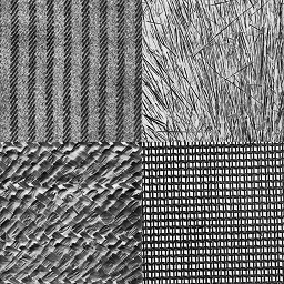
(a) Texture1

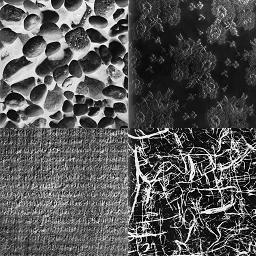
(b) Texture2

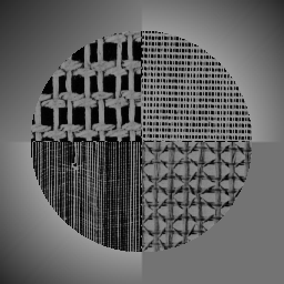
(c) Hybrid

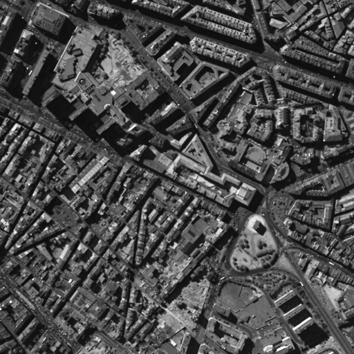
(d) Satellite1

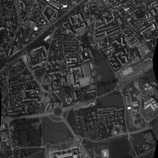
(e) Satellite2

Figure 1. Test images.

Now we report the numerical experiments of multiplicative noise removal for the original test images in Figure 1. All test images are corrupted by multiplicative Gamma noise with $L=4$ and the corresponding results are depicted in Figures 3-6. Figures 3 and 3 show the comparison of experimental results for two texture images. We find that Figures 3, 3 and 3, 3 lost more texture information in the images than Figures 3, 3 and 3, 3. Contrariwise, our model exhibits comparable performance to the F1P-AA model in removing noise, while surpassing it in preserving texture information. In the experiment which is shown in Figure 5, we utilize a test image that consists of textures and smooth surfaces. It is observed from Figures 5 and 5 that SO cause residual noise in homogeneous regions and AA fails to preserve texture information. Furthermore, our model performs better in preserving texture compared to the F1P-AA model, and also has favorable denoising effect across the entire image, avoiding the drawbacks of each model, see Figure 5 and Figure 5. As illustrated in Figures 5 and 6, the denoising results of the AA and F1P-AA model exhibit a certain degree of oversmoothing, while the results of the SO contain more residual noise. In comparison, although there are some isolated white speckle points in Figure 5 and Figure 6, our model achieves a balance between denoising effectiveness and texture preservation.

Table 1. Comparison of PSNR and SSIM of the different models for gamma noises with $L=1,4,10$.

	PSNR						SSIM
		Ours	SO	AA	F1P-AA	Ours	SO	AA	F1P-AA
$L=1$	Texture1	12.54	11.07	12.54	12.54	0.4289	0.4127	0.4357	0.4288
	Texture2	14.71	13.29	13.36	14.70	0.4488	0.4232	0.4298	0.4484
	Hybrid	18.34	14.41	16.78	18.33	0.5256	0.3394	0.5082	0.5258
	Satellite1	18.87	16.00	19.18	18.83	0.7091	0.6284	0.6985	0.6811
	Satellite2	22.74	19.10	23.21	22.70	0.6025	0.5520	0.6327	0.6000
$L=4$	Texture1	15.68	15.35	15.52	15.51	0.6885	0.6896	0.6845	0.6813
	Texture2	17.96	17.73	17.88	17.67	0.6933	0.6912	0.6917	0.6831
	Hybrid	21.19	20.28	19.16	20.44	0.6990	0.5467	0.6129	0.6309
	Satellite1	22.16	21.59	22.13	21.58	0.8681	0.8697	0.8567	0.8513
	Satellite2	25.42	24.71	25.39	24.73	0.8229	0.8204	0.8156	0.8056
$L=10$	Texture1	18.23	18.03	18.03	18.05	0.8170	0.8047	0.8141	0.8129
	Texture2	20.43	20.23	20.10	20.26	0.8133	0.8054	0.8076	0.8111
	Hybrid	23.61	23.42	22.71	22.62	0.7985	0.6082	0.7211	0.7229
	Satellite1	24.35	24.27	24.22	23.65	0.9280	0.9327	0.9230	0.9205
	Satellite2	27.47	27.23	27.30	26.91	0.9010	0.9008	0.8998	0.8959

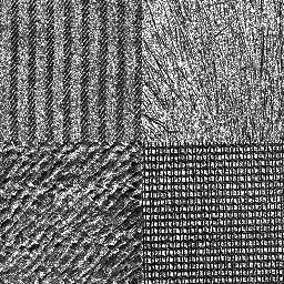
(a) Noisy: $L=4$

(b) Gabor

(c) Ours

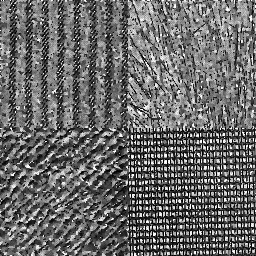
(d) SO

(e) AA

(f) F1P-AA

Figure 2. The texture1 image: (a) Noisy: $L=4$, PSNR $=13.7636$. (b) Gabor filtered noisy image. (c)-(f) Denoised results.

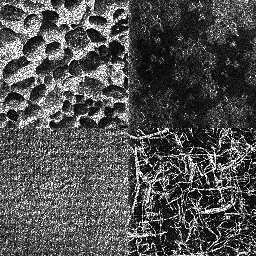
(a) Noisy: $L=4$

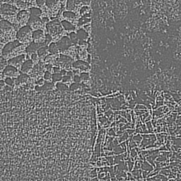
(b) Gabor

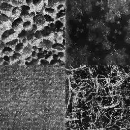
(c) Ours

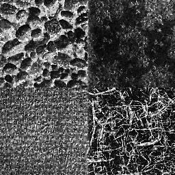
(d) SO

(e) AA

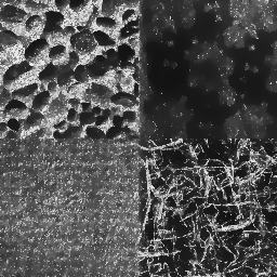
(f) F1P-AA

Figure 3. The texture2 image: (a) Noisy: $L=4$, PSNR $=15.5765$. (b) Gabor filtered noisy image. (c)-(f) Denoised results.

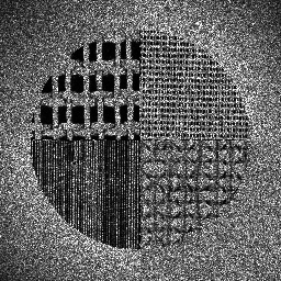
(a) Noisy: $L=4$

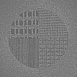
(b) Gabor

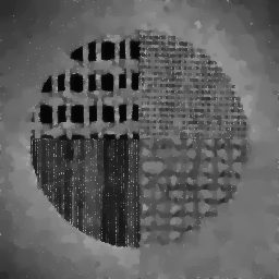
(c) Ours

(d) SO

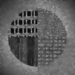
(e) AA

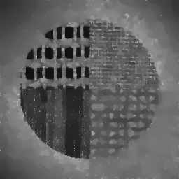
(f) F1P-AA

Figure 4. The hybrid image: (a) Noisy: $L=4$, PSNR $=14.3859$. (b) Gabor filtered noisy image. (c)-(f) Denoised results.

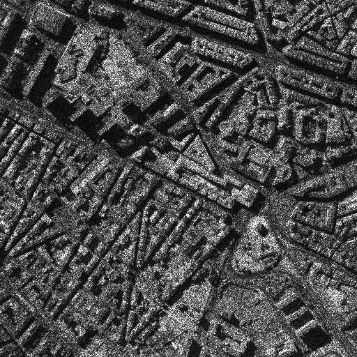
(a) Noisy: $L=4$

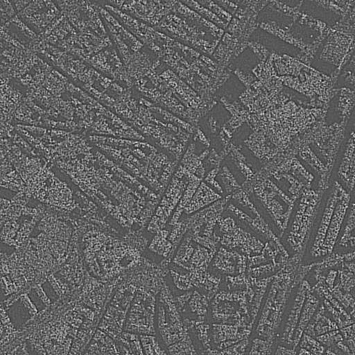
(b) Gabor

(c) Ours

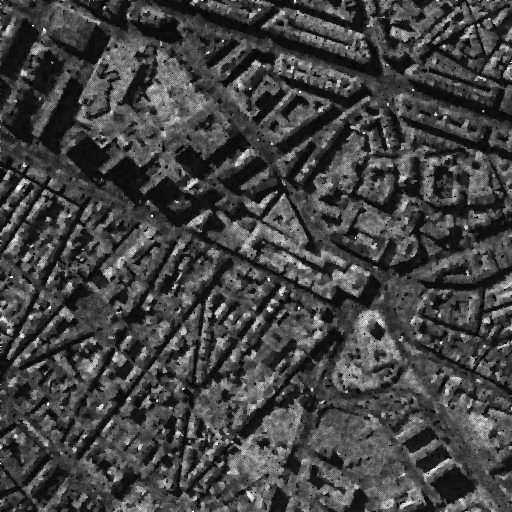
(d) SO

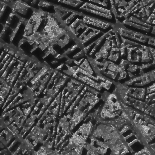
(e) AA

(f) F1P-AA

Figure 5. The satellite1 image: (a) Noisy: $L=4$, PSNR $=16.1315$. (b) Gabor filtered noisy image. (c)-(f) Denoised results.

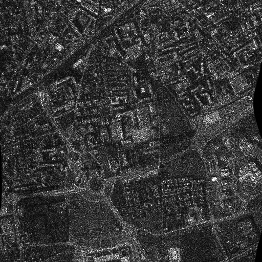
(a) Noisy: $L=4$

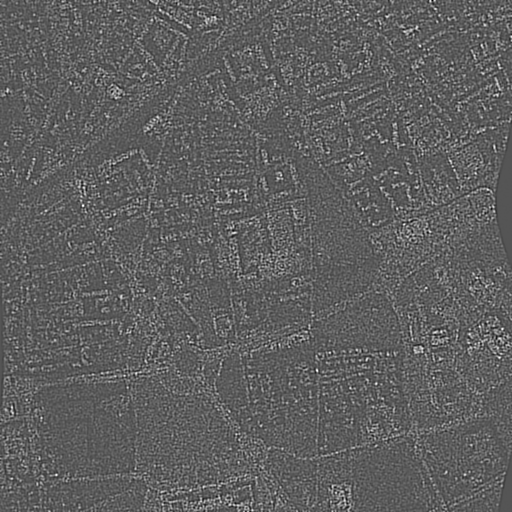
(b) Gabor

(c) Ours

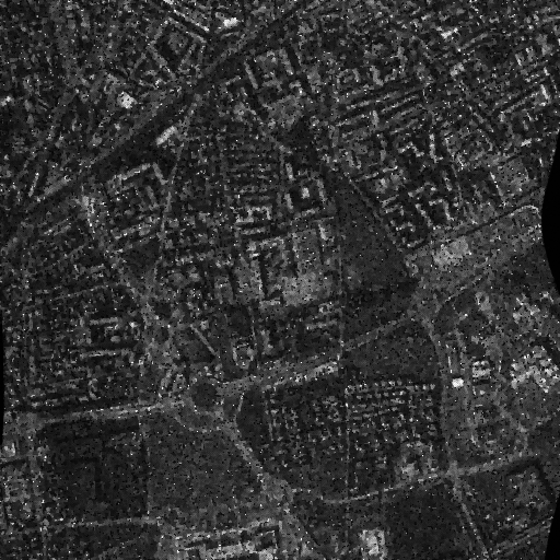
(d) SO

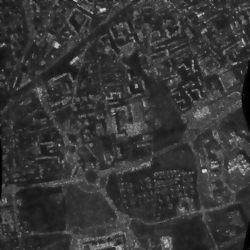
(e) AA

(f) F1P-AA

Figure 6. The satellite2 image: (a) Noisy: $L=4$, PSNR $=15.5765$. (b) Gabor filtered noisy image. (c)-(f) Denoised results.

References

- [1] B. Song, Topics in variational PDE image segmentation, inpainting and denoising, Ph.D. dissertation, University of California, Los Angeles (2003).
- [2] L. I. Rudin, S. Osher, E. Fatemi, Nonlinear total variation based noise removal algorithms, Physica D: Nonlinear Phenomena 60 (1) (1992) 259–268.
- [3] P. Perona, J. Malik, Scale-space and edge detection using anisotropic diffusion, IEEE Transactions on Pattern Analysis and Machine Intelligence 12 (7) (1990) 629–639.
- [4] F. Catté, P. L. Lions, J. M. Morel, T. Coll, Image selective smoothing and edge detection by nonlinear diffusion, SIAM Journal on Numerical Analysis 29 (1) (1992) 182–193.
- [5] Y. L. You, M. Kaveh, Fourth-order partial differential equations for noise removal, IEEE Transactions on Image Processing 9 (10) (2000) 1723–1730.
- [6] Y. Chen, S. Levine, M. Rao, Variable exponent, linear growth functionals in image restoration, SIAM Journal on Applied Mathematics 66 (4) (2006) 1383–1406.
- [7] Z. Guo, J. Sun, D. Zhang, B. Wu, Adaptive Perona–Malik model based on the variable exponent for image denoising, IEEE Transactions on Image Processing 21 (3) (2012) 958–967.
- [8] G. Aubert, J. F. Aujol, A variational approach to removing multiplicative noise, SIAM Journal on Applied Mathematics 68 (4) (2008) 925–946.
- [9] J. Shi, S. Osher, A nonlinear inverse scale space method for a convex multiplicative noise model, SIAM Journal on Imaging Sciences 1 (3) (2008) 294–321.
- [10] F. Li, M. K. Ng, C. Shen, Multiplicative noise removal with spatially varying regularization parameters, SIAM Journal on Imaging Sciences 3 (1) (2010) 1–20.
- [11] Z. Jin, X. Yang, A variational model to remove the multiplicative noise in ultrasound images, Journal of Mathematical Imaging and Vision 39 (1) (2011) 62–74.
- [12] G. Dong, Z. Guo, B. Wu, A convex adaptive total variation model based on the gray level indicator for multiplicative noise removal, Abstract and Applied Analysis 2013 (2013) 912373.
- [13] Z. Zhou, Z. Guo, G. Dong, J. Sun, D. Zhang, B. Wu, A doubly degenerate diffusion model based on the gray level indicator for multiplicative noise removal, IEEE Transactions on Image Processing 24 (1) (2015) 249–260.
- [14] Z. Zhou, Z. Guo, B. Wu, A doubly degenerate diffusion equation in multiplicative noise removal models, Journal of Mathematical Analysis and Applications 458 (1) (2018) 58–70.
- [15] Z. Zhou, Z. Guo, D. Zhang, B. Wu, A nonlinear diffusion equation-based model for ultrasound speckle noise removal, Journal of Nonlinear Science 28 (2) (2018) 443–470.
- [16] M. Gao, B. Kang, X. Feng, W. Zhang, W. Zhang, Anisotropic diffusion based multiplicative speckle noise removal, Sensors 19 (14) (2019).
- [17] X. Shan, J. Sun, Z. Guo, Multiplicative noise removal based on the smooth diffusion equation, Journal of Mathematical Imaging and Vision 61 (6) (2019) 763–779.
- [18] G. Gilboa, S. Osher, Nonlocal operators with applications to image processing, Multiscale Modeling & Simulation 7 (3) (2009) 1005–1028.
- [19] A. Buades, B. Coll, J. M. Morel, A review of image denoising algorithms, with a new one, Multiscale Modeling & Simulation 4 (2) (2005) 490–530.
- [20] S. Kindermann, S. Osher, P. W. Jones, Deblurring and denoising of images by nonlocal functionals, Multiscale Modeling & Simulation 4 (4) (2005) 1091–1115.
- [21] G. Gilboa, S. Osher, Nonlocal linear image regularization and supervised segmentation, Multiscale Modeling & Simulation 6 (2) (2007) 595–630.
- [22] F. Andreu, J. Mazón, J. Rossi, J. Toledo, A nonlocal -Laplacian evolution equation with neumann boundary conditions, Journal de Mathématiques Pures et Appliquées 90 (2) (2008) 201–227.
- [23] F. Andreu, J. M. Mazón, J. D. Rossi, J. Toledo, A nonlocal -Laplacian evolution equation with nonhomogeneous dirichlet boundary conditions, SIAM Journal on Mathematical Analysis 40 (5) (2009) 1815–1851.
- [24] J. M. Mazón, J. D. Rossi, J. Toledo, Fractional -Laplacian evolution equations, Journal de Mathématiques Pures et Appliquées 105 (6) (2016) 810–844.
- [25] J. P. Bouchaud, A. Georges, Anomalous diffusion in disordered media: Statistical mechanisms, models and physical applications, Physics Reports 195 (4) (1990) 127–293.
- [26] M. M. Meerschaert, A. Sikorskii, Stochastic Models for Fractional Calculus, De Gruyter, Berlin, Boston, 2012.
- [27] F. Lindgren, H. Rue, J. Lindström, An explicit link between Gaussian fields and Gaussian Markov random fields: the stochastic partial differential equation approach, Journal of the Royal Statistical Society: Series B (Statistical Methodology) 73 (4) (2011) 423–498.
- [28] N. Laskin, Fractional quantum mechanics and Lévy path integrals, Physics Letters A 268 (4) (2000) 298–305.
- [29] P. Gatto, J. S. Hesthaven, Numerical approximation of the fractional Laplacian via -finite elements, with an application to image denoising, Journal of Scientific Computing 65 (1) (2015) 249–270.
- [30] H. Antil, S. Bartels, Spectral approximation of fractional PDEs in image processing and phase field modeling, Computational Methods in Applied Mathematics 17 (4) (2017) 661–678.
- [31] Q. Liu, Z. Zhang, Z. Guo, On a fractional reaction–diffusion system applied to image decomposition and restoration, Computers & Mathematics with Applications 78 (5) (2019) 1739–1751.
- [32] T. Gao, Q. Liu, Z. Zhang, Fractional -Laplacian evolution equations to remove multiplicative noise, Discrete and Continuous Dynamical Systems - B 27 (9) (2022) 4837–4854.
- [33] C. Sutour, C. A. Deledalle, J. F. Aujol, Adaptive regularization of the NL-Means: Application to image and video denoising, IEEE Transactions on Image Processing 23 (8) (2014) 3506–3521.
- [34] J. Delon, A. Desolneux, C. Sutour, A. Viano, RNLp: Mixing nonlocal and TV-Lp methods to remove impulse noise from images, Journal of Mathematical Imaging and Vision 61 (4) (2019) 458–481.
- [35] A. Gárriz, F. Quirós, J. D. Rossi, Coupling local and nonlocal evolution equations, Calculus of Variations and Partial Differential Equations 59 (4) (2020) 112.
- [36] K. Shi, Coupling local and nonlocal diffusion equations for image denoising, Nonlinear Analysis: Real World Applications 62 (2021) 103362.
- [37] H. Antil, C. N. Rautenberg, Sobolev spaces with non-muckenhoupt weights, fractional elliptic operators, and applications, SIAM Journal on Mathematical Analysis 51 (3) (2019) 2479–2503.
- [38] M. Xiang, B. Zhang, D. Yang, Multiplicity results for variable-order fractional Laplacian equations with variable growth, Nonlinear Analysis 178 (2019) 190–204.
- [39] W. Bu, T. An, J. V. d. C. Sousa, Y. Yun, Infinitely many solutions for fractional -Laplacian Schrödinger–Kirchhoff type equations with symmetric variable-order, Symmetry 13 (8) (2021).
- [40] H. Brézis, Functional analysis, Sobolev spaces and partial differential equations, Springer New York, NY, 2011.
- [41] P. Bénilan, M. Crandall, Completely accretive operators, in: Semigroup theory and evolution equations, CRC Press, 1991, pp. 41–75.
- [42] F. Andreu, J. M. Mazón, J. D. Rossi, J. J. Toledo, Nonlocal diffusion problems, Vol. 165, American Mathematical Soc., 2010.
- [43] E. Di Nezza, G. Palatucci, E. Valdinoci, Hitchhiker’s guide to the fractional sobolev spaces, Bulletin des Sciences Mathématiques 136 (5) (2012) 521–573.
- [44] R. Hurri-Syrjänen, A. V. Vähäkangas, On fractional Poincaré inequalities, Journal d’Analyse Mathématique 120 (1) (2013) 85–104.
- [45] W. C. H. McLean, Strongly elliptic systems and boundary integral equations, Cambridge university press, 2000.
- [46] A. Fiscella, R. Servadei, E. Valdinoci, et al., Density properties for fractional sobolev spaces, Ann. Acad. Sci. Fenn. Math 40 (1) (2015) 235–253.
- [47] B. Manjunath, W. Ma, Texture features for browsing and retrieval of image data, IEEE Transactions on Pattern Analysis and Machine Intelligence 18 (8) (1996) 837–842.