Deep Equilibrium Diffusion Restoration with Parallel Sampling

Abstract

Diffusion-based image restoration (IR) methods aim to use diffusion models to recover high-quality (HQ) images from degraded images and achieve promising performance. Due to the inherent property of diffusion models, most of these methods need long serial sampling chains to restore HQ images step-by-step. As a result, it leads to expensive sampling time and high computation costs. Moreover, such long sampling chains hinder understanding the relationship between the restoration results and the inputs since it is hard to compute the gradients in the whole chains. In this work, we aim to rethink the diffusion-based IR models through a different perspective, i.e., a deep equilibrium (DEQ) fixed point system. Specifically, we derive an analytical solution by modeling the entire sampling chain in diffusion-based IR models as a joint multivariate fixed point system. With the help of the analytical solution, we are able to conduct single-image sampling in a parallel way and restore HQ images without training. Furthermore, we compute fast gradients in DEQ and found that initialization optimization can boost performance and control the generation direction. Extensive experiments on benchmarks demonstrate the effectiveness of our proposed method on typical IR tasks and real-world settings. The code and models will be made publicly available.

1 Introduction

Image restoration (IR) aims at recovering a high-quality image from a degraded input. Recently, Diffusion models [33, 56] are attracting more and more attention because they can generate higher quality images than GANs [19] and likelihood-based models [39]. Based on the diffusion models [33, 56], many IR methods [36, 16, 63] achieve compelling performance on different tasks. Directly using diffusion models in IR, however, suffers from some limitations.

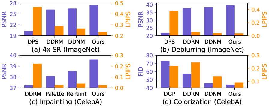
Figure 1: Comparisons of different diffusion-based zero-shot IR methods in various IR applications on different datasets.

First, diffusion-based IR models rely on a long sampling chain processing to synthesize high-quality images step-by-step, as shown in Figure 2 (a). As a result, it will lead to expensive sampling time during the inference. For example, DPS [16] based on DDPM [33] needs 1k sampling steps. To accelerate the sampling, some diffusion-based IR methods [36, 63, 80] use DDIM [56] to trade-off computation for sample quality. Based on this, these methods can reduce sampling steps to 100 or even less. Unfortunately, it may degrade the sample quality in the restoration when reducing the number of sampling steps [47]. It raises an interesting question: is it possible to use another way of sampling without sacrificing the sample quality?

Second, the long sampling chain makes understanding the relationship between the output restoration results and inputs to be difficult. In practice, many researchers notice that sampling different noise from Gaussian distribution as initialization may have different results. In this way, the diffusion models can generate diverse images. Such diversity is not necessary for some IR tasks, e.g., SR or deblurring. Nevertheless, different initialization may affect the performance of SR and deblurring. It raises the second question: is it possible to optimize the initialization such that the generation can be improved or stabilized? However, it is difficult for existing diffusion-based IR models to compute the gradient along the long sampling chain.

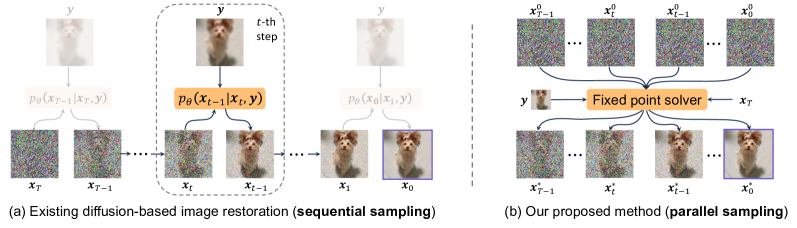
Figure 2: Comparisons of sequential sampling and our parallel sampling.

In this paper, we propose to rethink and analyze the sampling process of diffusion models in IR from the perspective of a deep equilibrium (DEQ) model [3]. We show that, surprisingly, it is possible to model the generative process of diffusion-based IR as DEQ, and call our method DeqIR. To this end, we first provide an analytical formulation of modeling all sampling steps as parallel sampling. Then, we solve DEQ to find the fixed point of all the sampling steps.

We summarize our contributions as follows:

• We prove that the long sampling chain in diffusion-based IR can be formulated in a parallel way. Then we analytically formulate the generative process as a deep equilibrium fixed point system. Moreover, the generation has a convergence guarantee with few timesteps and iterations.

• Compared with existing diffusion-based IR methods with sequential sampling, our method can achieve parallel sampling, as shown in Figure 2 (b). Moreover, our method can be run on multiple GPUs instead of a single GPU.

• Our model has more efficient gradients using DEQ inversion than existing diffusion-based IR methods which need a large computational graph for storing intermediate variables. The gradient can be computed through standard autograd packages. Moreover, we found that the initialization can be optimized with the gradients to improve the performance and control the generation direction.

• Extensive experiments on benchmarks demonstrate the effectiveness of our zero-shot method on different IR tasks, as shown in Figure 1. Moreover, our method performs well in real-world applications which may have unknown and non-linear degradations.

2 Related Work

Deep implicit learning.

Deep implicit learning attracts more and more attention and has emerging applications. Different from explicit learning, deep implicit learning is based on dynamical systems, e.g., optimization [1, 20, 23, 28, 57], differential equation [13, 24, 30], or fixed-point system [3, 4, 31]. Song et al.  [57] present a stochastic differential equation (SDE) and encapsulate previous approaches in score-based generative modeling and diffusion probabilistic modeling. For the fixed-point system, the deep equilibrium (DEQ) model [3] is a new type of implicit model. DEQ models sequential data by directly finding the fixed point and optimizing this equilibrium. Recently, DEQ has been widely used in different tasks, e.g., semantic segmentation [4], object detection [59, 60], robustness [70, 64, 41], optical flow estimation [5], and generative models like normalizing flow [46]. DEQ-DDIM [52] apply DEQs to diffusion models [33] by formulating this process as an equilibrium system. However, applying DEQs in diffusion-based IR methods is non-trivial because the generative process is complex, and formulating such a process is very challenging.

Diffusion-based image restoration. Previous image restoration (IR) methods [22, 22, 21] use CNN to achieve impressive performance on IR. Up to now, many researchers propose to design the architecture using residual blocks [37, 77, 10], GAN [32, 61, 62, 51, 49, 78], attention [79, 66, 17, 72, 71, 69, 73, 11, 43, 75, 42, 12, 44, 7, 9, 8], and others [68, 34, 25, 38, 26, 76] to improve the IR performance.

Recently, denoising diffusion probabilistic models (DDPM) [33] developed a powerful class of generative models that can generate high-quality images [19] from noise step-by-step. Based on the diffusion models, existing IR methods [36, 16, 63] can be divided into supervised methods and zero-shot methods. The supervised methods aim to train a conditional diffusion model in the image space [55, 65, 54, 74] or the latent space [53, 58, 67, 45]. However, these methods need training diffusion models for the image inverse problem and have limited generalization performance to different degradations in different IR tasks.

For zero-shot IR methods, DDRM [36] applies a pre-trained denoising diffusion generative model to solve a linear inverse problem with 20 sampling steps. Each step uses singular value decomposition (SVD) on the degradation operator. However, SVD has an expensive cost for memory and computation when the dimension of the degradation matrix is very high. DPS [16] solves the inverse problems via approximation of the posterior sampling using 1000 steps of the manifold-constrained gradient. Similarly to DPS, DiffPIR [80] integrates the traditional plug-and-play method into the diffusion models. DDNM [63] applies range-null space decomposition in linear image inverse problem and refine the Null-space iteratively. DDNM uses DDIM as the base sampling strategy with 100 sampling steps. Based on a given reference image, ILVR [15] guides the generative process in DDPM and generates high-quality images. Repaint [48] also employs a pre-trained DDPM as the generative prior for the image inpainting task. However, all of these methods use the serial sampling chain, resulting in a long sampling time.

3 Preliminaries

Image restoration.

Image restoration aims at synthesizing high-quality image $\hat{{\bm{x}}}$ from a degraded observation ${\bm{y}}={\bm{A}}\left({{\bm{x}}}\right)+{\bm{n}}$, where ${\bm{A}}$ is some degradation (e.g., bicubic), ${\bm{x}}$ is the original image, and ${\bm{n}}$ is a non-linear noise (e.g., white Gaussian noise) with the level $\sigma$. The solution can be obtained by optimizing the following problem:

$$\hat{{\bm{x}}}=\operatorname*{arg\,min}\nolimits_{{\bm{x}}}{1}/{2\sigma^{2}}\left\|{\bm{A}}({\bm{x}})-{\bm{y}}\right\|_{2}^{2}+\lambda{\mathcal{R}}({\bm{x}}),$$ (1)

where ${\mathcal{R}}({\bm{x}})$ is a reguralization with a trade-off parameter $\lambda$, e.g., sparsity and Tikhonov regularization.

Diffusion models. DDPM [33] is a latent variable model that can synthesize high-quality image results with a forward process (i.e., diffusion process) and a reverse process. The forward process is a Markov chain that gradually introduces Gaussian noise with specific noise levels to the data,

$$q({\bm{x}}_{t}|{\bm{x}}_{0})={\mathcal{N}}\left({\bm{x}}_{t};\sqrt{\bar{\alpha}_{t}}{\bm{x}}_{0},(1-\bar{\alpha}_{t}){\bm{I}}\right),$$ (2)

where $\bar{\alpha}_{t}:=\Pi_{s=1}^{t}\alpha_{s}$, $\alpha_{t}:=1-\beta_{t}$ and $\beta_{t}$ is a variance. For the reverse process, the previous state ${\bm{x}}_{t-1}$ can be predicted with $\tilde{{\bm{\mu}}}_{t}$ and $\tilde{\sigma}_{t}$, i.e.,

$$q({\bm{x}}_{t-1}|{\bm{x}}_{t},{\bm{x}}_{0})={\mathcal{N}}\left({\bm{x}}_{t-1};\tilde{{\bm{\mu}}}_{t}({\bm{x}}_{t},{\bm{x}}_{0}),\tilde{\sigma}_{t}^{2}{\bm{I}}\right),$$ (3)

where $\tilde{{\bm{\mu}}}_{t}({\bm{x}}_{t},{\bm{x}}_{0}):=\frac{\sqrt{\bar{\alpha}_{t-1}}\beta_{t}}{1-\bar{\alpha}_{t}}{\bm{x}}_{0}+\frac{\sqrt{\alpha_{t}}(1-\bar{\alpha}_{t-1})}{1-\bar{\alpha}_{t}}{\bm{x}}_{t}=\frac{1}{\sqrt{{\alpha}_{t}}}({\bm{x}}_{t}-\frac{1-\alpha_{t}}{\sqrt{1-\bar{\alpha}_{t}}}\mbox{{\boldmath$\epsilon$}})$ and $\tilde{\sigma}_{t}^{2}:=\frac{1{-}\bar{\alpha}_{t{-}1}}{1{-}\bar{\alpha}_{t}}\beta_{t}$. Here, the noise $\mbox{{\boldmath$\epsilon$}}\sim{\mathcal{N}}(0,{\bm{I}})$ can be estimated by $\mbox{{\boldmath$\epsilon$}}_{\theta}({\bm{x}}_{t},t)$ in each time-step. To apply $\tilde{{\bm{\mu}}}_{t}$ to the image inverse problem, one can replace ${\bm{x}}_{0}$ with $\hat{{\bm{x}}}_{0|t}$ conditioned on the degraded image ${\bm{y}}$, i.e.,

$${\bm{x}}_{t-1}=\frac{\sqrt{\bar{\alpha}_{t-1}}\beta_{t}}{1-\bar{\alpha}_{t}}\hat{{\bm{x}}}_{0|t}+\frac{\sqrt{\bar{\alpha}_{t}}(1-\bar{\alpha}_{t-1})}{1-\bar{\alpha}_{t}}{\bm{x}}_{t}+\sigma_{t}\mbox{{\boldmath$\epsilon$}},$$ (4)

where $\hat{{\bm{x}}}_{0|t}$ can be estimated by using a degradation ${\bm{A}}$ to map the denoised image ${\bm{x}}_{0|t}=\frac{1}{\sqrt{\bar{\alpha}_{t}}}({\bm{x}}_{t}-\sqrt{1-\bar{\alpha}_{t}}\mbox{{\boldmath$\epsilon$}}_{\theta}({\bm{x}}_{t},t))$ in the degradation space [63], i.e.,

$$\hat{{\bm{x}}}_{0|t}={\bm{A}}^{{\dagger}}{\bm{y}}+({\bm{I}}-{\bm{A}}^{{\dagger}}{\bm{A}}){\bm{x}}_{0|t},$$ (5)

where ${\bm{A}}^{{\dagger}}$ is the pseudo-inverse of ${\bm{A}}$.

Deep equilibrium models. Deep equilibrium models (DEQs) [3] are infinite depth feed-forward networks that can find fixed points in the forward pass. Given an input injection ${\bm{x}}$, an hidden state $\mbox{{\boldmath$\nu$}}^{k+1}$ can be predict by using a equilibrium layer $f_{\theta}$ parametrized by $\theta$, i.e.,

$$\mbox{{\boldmath$\nu$}}^{k+1}=f_{\theta}\left(\mbox{{\boldmath$\nu$}}^{k};{\bm{x}}\right),k=0,\ldots,L{-}1.$$ (6)

When increasing the depth towards infinity, the model tend to converge to a fixed point (equilibrium) $\mbox{{\boldmath$\nu$}}^{*}$, i.e.,

$$\lim\limits_{k\to\infty}f_{\theta}\left(\mbox{{\boldmath$\nu$}}^{k};{\bm{x}}\right)=f_{\theta}\left(\mbox{{\boldmath$\nu$}}^{*};{\bm{x}}\right)=\mbox{{\boldmath$\nu$}}^{*}.$$ (7)

To solve the equilibrium state $\mbox{{\boldmath$\nu$}}^{*}$, one can use some fixed point solvers, like Broyden’s method [6], or Anderson acceleration [2], and it can be accelerated by the neural solver [13] in the inference. More details are put in Supplementary.

4 Methodology

4.1 Deep Equilibrium Diffusion Restoration

Existing zero-shot image restoration methods [16, 36, 63] restore high-quality images step-by-step with long serial sampling chains. Such an inherent property comes from the diffusion models, and it will lead to expensive sampling time and high computation costs. This issue may be intractable if we need a gradient by backpropagating through the long sampling chains which often results in out-of-memory in the experiments. To address this, we propose the main modeling contribution of this paper.

Fixed point modeling. Motivated by [52], our goal is to formulate diffusion models as a deep equilibrium fixed point system. Specifically, given a degraded image ${\bm{y}}$ and Gaussian noise image ${\bm{x}}_{T}$, the sampling chain ${\bm{x}}_{0:T-1}$ can be treated as multivariable of the DEQ fixed point system, we first formulate the ${\bm{x}}_{0:T{-}1}$ as follows:

$${\bm{x}}_{0:T-1}=F({\bm{x}}_{0:T-1};({\bm{x}}_{T},{\bm{y}})),$$ (8)

where ${\bm{x}}_{T}\sim{\mathcal{N}}({\bf 0},{\bm{I}})$ and the degraded image ${\bm{y}}$ are the input injections, and $F(\cdot)$ is the function that performs sequential data across all the sample steps simultaneously. To formulate the function $F$ in Eqn. (8), we first provide the following proposition for parallel sampling.

Proposition 1.

(Parallel sampling) Given a degradation matrix ${\bm{A}}$, a degraded image ${\bm{y}}$ and a Gaussian noise image ${\bm{x}}_{T}\sim{\mathcal{N}}({\bf 0},{\bm{I}})$, for $k\in[1,\ldots,T]$, the state ${\bm{x}}_{T-k}$ can be predicted by previous states $\{{\bm{x}}_{T-k+1},\ldots,{\bm{x}}_{T}\}$, i.e.,

$${\bm{x}}_{T-k}= \frac{\sqrt{\bar{\alpha}_{T-k}}}{\sqrt{\bar{\alpha}_{T}}}\left({\bm{I}}-{\bm{A}}^{\dagger}{\bm{A}}\right){\bm{x}}_{T}+{\bm{A}}^{\dagger}{\bm{A}}{\bm{z}}_{T-k+1}$$ (9)

$$+\sum_{s=T-k}^{T-1}\frac{\sqrt{\bar{\alpha}_{T-k}}}{\sqrt{\bar{\alpha}_{s}}}\left({\bm{I}}-{\bm{A}}^{\dagger}{\bm{A}}\right){\bm{z}}_{s+1},$$

where ${\bm{z}}_{s}=c_{t}^{0}\mbox{{\boldmath$\epsilon$}}_{\theta}({\bm{x}}_{s},{s})+\sqrt{\bar{\alpha}_{t-1}}{\bm{y}}+c_{t}^{1}{\bm{x}}_{T}$, the coefficients are defined as $c_{t}^{0}:=c_{t}^{2}-\sqrt{(1-\bar{\alpha}_{t})/{\alpha}_{t}}({\bm{I}}-{\bm{A}}^{\dagger}{\bm{A}})$, $c_{t}^{1}:=\sqrt{1-\bar{\alpha}_{t}}\eta$, $c_{t}^{2}:=\sqrt{1-\bar{\alpha}_{t}}\sqrt{1-\eta^{2}},0\leq\eta<1$.

Proof.

Please refer to the proofs in Supplementary.

From the proposition, ${\bm{x}}_{T-k}$ is related to subsequent states ${\bm{x}}_{T-k+1:T}$ and the degraded image ${\bm{y}}$. Different from existing diffusion-based image restoration methods which update ${\bm{x}}_{t}$ based only on ${\bm{x}}_{t+1}$. The timestep $T$ can be small with the help of DDIM [56]. In Eqn. (9), we need a known degradation matrix ${\bm{A}}$ in the image inverse problem. When the degradation matrix ${\bm{A}}$ is unknown in the real-world application, one can use its approximation version in practice. In addition, the performance is related to the hyper-parameter $\eta$. We investigate the effect of the hyper-parameter $\eta$ on the performance in the experiments.

Based on our proposed proposition, we can formulate the right side of Eqn. (9) as ${\bm{x}}_{T-k}=f({\bm{x}}_{T-k+1:T};{\bm{y}})$. Then, we can write all sampling steps as a ”fully-lower-triangular” inference process, i.e.,

$$\begin{bmatrix}{\bm{x}}_{T{-}1}\\ {\bm{x}}_{T{-}2}\\ \vdots\\ {\bm{x}}_{0}\end{bmatrix} =\begin{bmatrix}f({\bm{x}}_{T};{\bm{y}})\\ f({\bm{x}}_{T{-}1:T};{\bm{y}})\\ \vdots\\ f({\bm{x}}_{1:T};{\bm{y}}).\\ \end{bmatrix}$$ (10)

The function $f$ in Eqn. (10) can be implemented in all sequential states in parallel, corresponding to Eqn. (8), i.e., ${\bm{x}}_{0:T-1}=F({\bm{x}}_{0:T-1};({\bm{x}}_{T},{\bm{y}}))$. To find the solution to the fixed point of Eqn. (10), we apply commonly used fixed point solvers like Anderson acceleration [2] which can accelerate the convergence of the fixed-point sequence. To this end, we first define the residual $g({\bm{x}}_{0:T-1};({\bm{x}}_{T},{\bm{y}}))=F({\bm{x}}_{0:T-1};({\bm{x}}_{T},{\bm{y}}))-{\bm{x}}_{0:T-1}$. Then, we can directly input the residual to the Anderson acceleration and obtain the final converged fixed point, i.e.,

$${\bm{x}}_{0:T-1}^{*}=\mathrm{RootSolve}\left(g({\bm{x}}_{0:T-1};({\bm{x}}_{T},{\bm{y}}))\right),$$ (11)

where ${\bm{x}}_{0}^{*}$ is our desired result at the end of sampling, and $\mathrm{RootSolve}(\cdot)$ is a solver using Anderson acceleration for fixed-point iterations. We define $g_{k}:=g({\bm{x}}_{0:T-1}^{(k)};({\bm{x}}_{T},{\bm{y}}))$ and provide the detailed implementation in Algorithm 1 in which the formulation of $F$ is our main contribution. Note that $\mathrm{RootSolve}(\cdot)$ is implemented in PyTorch package [52], and we use the same hyper-parameters as [52]. Moreover, Algorithm 1 is guaranteed to converge to a fixed point, which is verified in the following experiments.

Algorithm 1 Implementation of $\mathrm{RootSolve}(\cdot)$

Require: A degraded image ${\bm{y}}$, a pre-trained diffusion model, timesteps $T$, iterations $K$, an integer parameter $m\geq 1$

1:Initialize $\mathbf{x}_{0:T-1}^{(0)},{\bm{x}}_{T}\sim\mathcal{N}(\mathbf{0},\mathbf{I})$

2:$\mathbf{x}_{0:T-1}^{(1)}=F(\mathbf{x}_{0:T-1}^{(0)};({\bm{x}}_{T},{\bm{y}}))$

3:for $k$ from $1$ to $K$ do

4:     $m_{k}=\min\{m,k\}$

5:     ${\bm{G}}_{k}=[g_{k-m_{k}},\ldots,g_{k}]$

6:     Solve least-squares problem for ${\bm{\alpha}}{=}[\alpha_{0},\ldots,\alpha_{m_{k}}]$

$${\bm{\alpha}}_{k}=\operatorname*{arg\,min}\nolimits_{{\bm{\alpha}}}\|{\bm{G}}_{k}{\bm{\alpha}}\|_{2},s.t.,{\bm{\alpha}}^{\top}{\bf 1}=1$$

7:     Update the sequence

$${\bm{x}}_{0:T-1}^{(k+1)}=\sum\nolimits_{i=0}^{m_{k}}({\bm{\alpha}}_{k})_{i}F\left({\bm{x}}_{0:T-1}^{(k-m_{k}+i)};\left({\bm{x}}_{T},{\bm{y}}\right)\right)$$

8:end for

9:return $\mathbf{x}_{0}^{K}$

Compared with most existing diffusion-based IR methods [16, 63], our method operating all states in parallel results in more accurate estimations of the intermediate latent states ${\bm{x}}_{t}$, requiring fewer sampling steps. It implies that we are able to obtain the better final sample ${\bm{x}}_{0}^{*}$ based on these accurate estimated intermediate latent states ${\bm{x}}_{t}$.

Algorithm 2 Initialization Optimization via DEQ inversion

Require: A degraded image ${\bm{y}}$, a pre-trained diffusion model, update rate $\lambda$, total steps $S$.

1:$\mathbf{x}_{0:T}\sim\mathcal{N}(\mathbf{0},\mathbf{I})$

2:for steps from $1$ to $S$ do

3:     Disable gradient computation, and compute ${\bm{x}}_{0:T-1}^{*}$ according to Algorithm 1,

$${\bm{x}}_{0:T-1}^{*}=\mathrm{RootSolve}\left(g({\bm{x}}_{0:T-1};({\bm{x}}_{T},{\bm{y}}))\right)$$

4:     Enable gradient computation, and compute loss and use the 1-step grad $\partial{\mathcal{L}}/\partial{\bm{x}}_{T}$

5:     Update ${\bm{x}}_{T}$ with a gradient descent:

$${\bm{x}}_{T}\leftarrow{\bm{x}}_{T}+\lambda\partial{\mathcal{L}}/\partial{\bm{x}}_{T}$$

6:end for

7:return $\mathbf{x}^{T}$

4.2 Initialization Optimization via DEQs Inversion

Existing diffusion-based IR methods [16, 63] notice that different initializations have diverse generations in some IR tasks, e.g., colorization and inpainting. However, such diversity of generation is hard to control, and it is harmful to SR or deblurring which requires guaranteeing the identity. To address this, we provide an interesting perspective to explore the initialization of our diffusion model.

To achieve this, we first define a general loss function that can provide additional information. Specifically, given a degraded image ${\bm{y}}$ and the output of $\mathrm{RootSolve}$ (i.e., ${\bm{x}}_{0}^{*}$), then the loss can be defined as

$${\mathcal{L}}=\ell\left(\phi({\bm{x}}_{0}^{*}),\varphi({\bm{y}})\right),$$ (12)

where $\ell$ can be $L_{2}$ loss or perceptual loss. For example, $\phi$ can be ${\bm{A}}$ and $\varphi$ is an identity function; or $\phi$ is an identity function and $\varphi$ is a pre-trained IR model [43, 14]. Based on the loss, we apply the implicit function theorem (IFT) to compute the gradients of the loss ${\mathcal{L}}$ w.r.t. ${\bm{x}}_{T}$, i.e.,

$$\dfrac{\partial\mathcal{L}}{\partial{\bm{x}}_{T}}=-\dfrac{\partial\mathcal{L}}{\partial{\bm{x}}^{*}_{0:T}}\left(J_{g}^{-1}\big{|}_{{\bm{x}}^{*}_{0:T}}\right)\dfrac{\partial F({\bm{x}}^{*}_{0:T-1};{\bm{x}}_{T})}{\partial{\bm{x}}_{T}},$$ (13)

where $J_{g}^{-1}\big{|}_{{\bm{x}}^{*}_{0:T}}$ is the inverse Jacobian of $g({\bm{x}}_{0:T-1};{\bm{x}}_{T})$ evaluated at ${\bm{x}}_{0:T}^{*}$. In practical, we use an approximation version, i.e., ${\bm{M}}\approx J_{g}^{-1}|_{{\bm{x}}^{*}_{0:T}}$, e.g., 1-step gradient (i.e., ${\bm{M}}={\bm{I}}$) [27, 28, 29]. Note that the pre-trained diffusion model is frozen. The gradients can be computed by using standard autograd packages in PyTorch. Then, ${\bm{x}}_{T}$ can be updated along the gradient, as shown in Algorithm 2.

Different from existing diffusion-based IR methods which have a large computational graph to store the gradients in the whole process, our method is more efficient by using the DEQ inversion. In addition, with the help of the inversion method, our zero-shot IR methods can be extended to supervised learning by replacing the loss (12) with ${\mathcal{L}}=\|{\bm{x}}_{0}^{*}-{\bm{x}}_{0}\|_{F}^{2}$ which we leave it in the future work.

Datasets	Methods	2$\times$SR			4$\times$SR			Deblur (gauss)			Deblur (aniso)			NFEs/Iters
		PSNR↑	​​​​​​SSIM↑​​​​​​	LPIPS↓	PSNR↑	​​​​​​SSIM↑​​​​​​	LPIPS↓	PSNR↑	​​​​​​SSIM↑​​​​​​	LPIPS↓	PSNR↑	​​​​​​SSIM↑​​​​​​	LPIPS↓
ImageNet	Baseline	29.63	​​​​0.875​​​​	0.165	25.15	​​​​0.699​​​​	0.351	18.22	​​​​0.529​​​​	0.433	20.86	​​​​0.544​​​​	0.480	-
	DGP [50]	22.32	​​​​0.583​​​​	0.426	18.35	​​​​0.398​​​​	0.529	21.81	​​​​0.522​​​​	0.472	20.77	​​​​0.459​​​​	0.504	1500
	DPS [16]	22.40	​​​​0.597​​​​	0.405	20.34	​​​​0.488​​​​	0.464	22.04	​​​​0.569​​​​	0.394	21.82	​​​​0.561​​​​	0.381	1000
	ILVR [15]	23.36	​​​​0.613​​​​	0.334	22.76	​​​​0.583​​​​	0.383	-	-	-	-	-	-	100
	DiffPIR [80]	27.16	​​​​0.790​​​​	0.214	24.31	​​​​0.649​​​​	0.350	25.32	​​​​0.673​​​​	0.296	23.37	​​​​0.535​​​​	0.439	100
	DDRM [36]	31.43	​​​​0.906​​​​	0.117	26.21	​​​​0.745​​​​	0.288	40.70	​​​​0.978​​​​	0.040	37.69	​​​​0.964​​​​	0.057	20
	DDNM [63]	31.81	​​​​0.908​​​​	0.096	26.49	​​​​0.753​​​​	0.266	43.83	​​​​0.987​​​​	0.021	38.40	​​​​0.969​​​​	0.039	100
	DeqIR (Ours)	32.33	​​​​0.913​​​​	0.081	27.44	​​​​0.782​​​​	0.235	43.55	​​​​0.987​​​​	0.020	39.47	​​​​0.970​​​​	0.036	15
CelebA-HQ	Baseline	35.87	​​​​0.953​​​​	0.099	30.12	​​​​0.857​​​​	0.240	18.94	​​​​0.704​​​​	0.337	23.16	​​​​0.727​​​​	0.354	-
	DGP [50]	28.61	​​​​0.809​​​​	0.279	25.25	​​​​0.690​​​​	0.405	27.02	​​​​0.738​​​​	0.372	25.73	​​​​0.663​​​​	0.426	1500
	DPS [16]	28.71	​​​​0.818​​​​	0.219	25.01	​​​​0.710​​​​	0.282	27.56	​​​​0.775​​​​	0.229	26.91	​​​​0.754​​​​	0.234	1000
	ILVR [15]	27.31	​​​​0.783​​​​	0.234	27.09	​​​​0.775​​​​	0.245	-	-	-	-	-	-	100
	DiffPIR [80]	32.51	​​​​0.882​​​​	0.156	28.60	​​​​0.795​​​​	0.228	30.63	​​​​0.835​​​​	0.197	29.32	​​​​0.802​​​​	0.232	100
	DDRM [36]	36.76	​​​​0.952​​​​	0.074	31.91	​​​​0.880​​​​	0.149	43.06	​​​​0.983​​​​	0.036	41.27	​​​​0.976​​​​	0.053	20
	DDNM [63]	36.37	​​​​0.950​​​​	0.065	31.86	​​​​0.876​​​​	0.136	46.99	​​​​0.992​​​​	0.021	43.43	​​​​0.983​​​​	0.037	100
	DeqIR (Ours)	36.57	​​​​0.953​​​​	0.061	32.19	​​​​0.887​​​​	0.154	47.46	​​​​0.993​​​​	0.019	43.58	​​​​0.984​​​​	0.035	15

Table 1: Quantitative results of zero-shot IR methods on ImageNet and CelebA, including super-resolution and deblurring. Best results are highlighted as ​first​, ​second​ and ​third​.

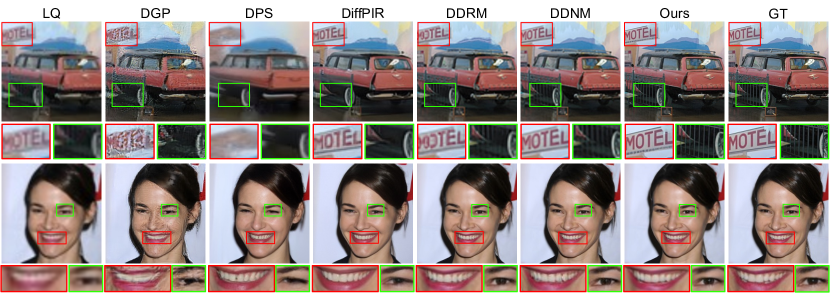
Figure 3: Qualitative results of zero-shot $4{\times}$ super-resolution methods on ImageNet and CelabA-HQ.

5 Experiments

Experiment settings. We conduct the following typical IR tasks, including super-resolution (SR), deblurring, colorization, and inpainting. Specifically, we consider 4$\times$ and 2$\times$ bicubic downsampling for SR, Gaussian, and Anisotropic for deblurring, use an average grayscale operator in colorization, and use text and stripe masks in inpainting. For convenience, we choose ImageNet [18] and CelebA-HQ [35] datasets with 100 classes [80] and the image size $256{\times}256$ for validation, which have the same trend on 1k classes. For fair comparisons, we use the same pre-trained diffusion models [19] and [48] for ImageNet and CelebA-HQ, respectively. More experiment details are put in Supplementary Materials.

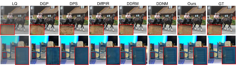
Figure 4: Qualitative results of zero-shot image deblurring (gauss) methods.

Methods	Text mask			Stripe mask
	PSNR↑	​​​​​​​​​​SSIM↑​​​​​​​​​​	LPIPS↓	PSNR↑	​​​​​​​​​​SSIM↑​​​​​​​​​​	LPIPS↓
Baseline	14.55	​​​​​​0.642​​​​​​	0.515	9.02	​​​​​​0.131​​​​​​	0.730
Palette [54]	38.09	​​​​​​0.978​​​​​​	0.027	25.91	​​​​​​0.733​​​​​​	0.343
RePaint [48]	38.54	​​​​​​0.974​​​​​​	0.039	36.25	​​​​​​0.950​​​​​​	0.087
DDRM [36]	37.25	​​​​​​0.969​​​​​​	0.223	34.34	​​​​​​0.933​​​​​​	0.223
DDNM [63]	39.45	​​​​​​0.980​​​​​	0.023	36.75	​​​​​​0.951​​​​​​	0.076
DeqIR (Ours)	39.60	​​​​​​0.981​​​​​	0.026	36.97	​​​​​​0.952​​​​​	0.086

Table 2: Comparisons of zero-shot inpainting methods on CelebA.

Methods	ImageNet			CelebA-HQ
	Cons↓	​​​​​​​​​​LPIPS↓​​​​​​​​​​	FID↓	Cons↓	​​​​​​​​​​LPIPS↓​​​​​​​​​​	FID↓
Baseline	0	​​​​​​0.196​​​​​​	90.93	0	​​​​​​0.210​​​​​​	70.69
DGP [50]	-	​​​​​​0.256​​​​​​	99.86	-	​​​​​​0.218​​​​​​	73.24
DDRM [36]	265.08	​​​​​​0.223​​​​​​	79.42	472.25	​​​​​​0.245​​​​​​	57.29
DDNM [63]	45.07	​​​​​​0.186​​​​​	77.21	51.43	​​​​​​0.139​​​​​	45.73
DeqIR (Ours)	43.15	​​​​​​0.171​​​​​	70.94	50.16	​​​​​​0.092​​​​​	43.98

Table 3: Quantitative results of zero-shot colorization methods.

Evaluation metrics. We use PSNR, SSIM, and LPIPS as the evaluation metrics for most image restoration tasks. In general, higher PSNR and SSIM, and lower LPIPS and FID mean better performance. For the task of colorization, we use the Consistency metric [63] and FID because PSNR and SSIM cannot reflect the performance [63]. We report the number of NFEs (timesteps) or iterations for each method.

5.1 Evaluation on Image Super-Resolution

We compare our method with a GAN-based IR method (e.g., DGP) and SOTA zero-shot diffusion-based IR methods (DPS [16], DiffPIR [80], DDRM [36] and DDNM [63]) on ImageNet and CelebA-HQ datasets. In addition, we show bicubic upscaling as a baseline for SR.

The quantitative results are shown in Table 1. We can see that our method outperforms most methods under different metrics on both ImageNet and CelebA-HQ. In particular, compared with the competitive IR method DDNM, our method on ImageNet surpasses it by LPIPS margin of up to 0.031, and by PSNR margin of up to 0.95dB. Moreover, our method only needs 15 sampling steps, compared with DDNM (100 steps). We provide more quantitative results of other scales in Supplementary Materials.

For the qualitative results, our method has the best visual quality containing more realistic textures, as shown in Figure 3. These visual comparisons align with the quantitative results, demonstrating the effectiveness of our method. More visual results are put in Supplementary Materials.

5.2 Evaluation on Image Deblurring

We compare the same zero-shot IR methods used in the SR task. In addition, we use ${\bm{A}}^{{\dagger}}{\bm{y}}$ as a baseline. In this experiment, we mainly consider Gaussian and anisotropic kernels to evaluate the performance of all models.

In Table 1, the quantitative results show that our method achieves the best performance on all datasets, except for PSNR of Gaussian deblurring on ImageNet. Compared with DDNM [63], the PSRN improvement of our method can be up to 1.07dB for anisotropic kernel deblurring. In Figure 4, our generated images have the best visual quality with more realistic details which are close to GT images. We provide more quantitative and qualitative results (including more kernels) in Supplementary Materials.

5.3 Evaluation on Image Inpainting

For the image inpainting task, we compare our method with SOTA inpainting methods, including Palette [54], RePaint [48], DDRM [36], and DDNM [63]. We also use ${\bm{A}}^{{\dagger}}{\bm{y}}$ as a baseline. In addition, we consider the text mask and stripe mask as examples and show the results on CelebA-HQ in Table 3. The results of more masks and the results on ImageNet are put in the supplementary materials.

In Table 3, our method outperforms most diffusion models (i.e., Palette [54], RePaint [48] and DDRM [36]) significantly, and has comparable performance with DDNM [63]. In Figure 6, taking the mouth in the generated face images as an example, our method generates structures and details that are not only more realistic but also more reasonable compared to other inpainting methods. Further qualitative results are available in Supplementary Materials.

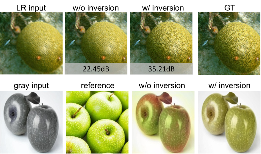
Figure 5: Interesting applications of DEQ inversion.

5.4 Evaluation on Image Colorization

We compare our method with SOTA methods (i.e., DGP [50], DDRM [36], and DDNM [63]). We also use i.e., ${\bm{A}}^{{\dagger}}{\bm{y}}$ as a baseline. In addition to LPIPS, we additionally use the Consistency metric and FID to evaluate the image quality.

In Table 5, our method achieves the best performance on both ImageNet and CelebA-HQ under different metrics. As shown in Figure 7, we can see that our method restores images with reasonable color. In contrast, other methods may restore part color (see the tree) or unreasonable color (e.g., in the building in DGP [50]).

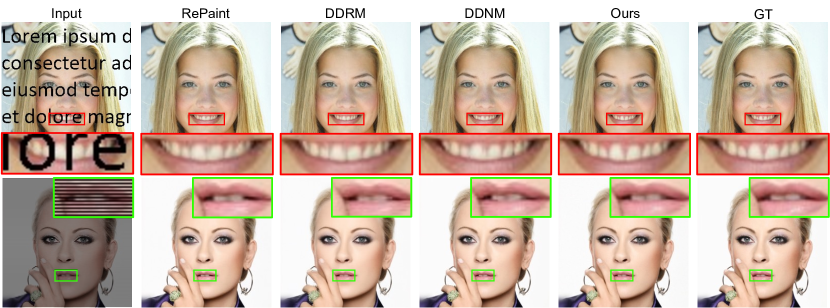
Figure 6: Qualitative results of image inpainting methods on CelebA-HQ.

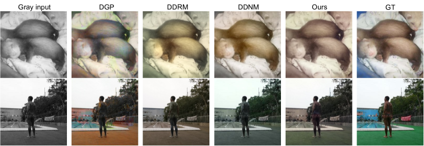
Figure 7: Qualitative results of image colorization methods on ImageNet.

5.5 Evaluation on DEQs Inversion

We extend our method using DEQs inversion to interesting applications, e.g., SR with optimized initialization (top) and reference-based colorization (bottom), as shown in Figure 5. We found that optimizing the initialization is able to improve PSNR and control the generation to the desired direction. More details and results are put in Supplementary.

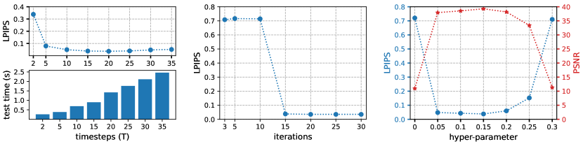
Figure 8: Ablation study of timesteps (left), iteration (middle) and hyper-parameters (right) for anisotropic deblurring on ImageNet.

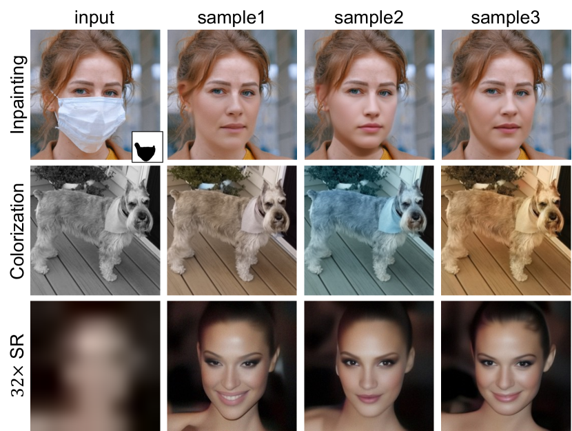
Figure 9: Diversity of generation of our method.

5.6 Ablation Study

Effect of timesteps. We study the impact of timesteps in our diffusion models. Specifically, we change the number of timesteps from 2 to 35. In Figure 8 (left), our model achieves better performance with more timesteps. However, more timesteps lead to a larger memory and slower convergence. To trade-off the performance and efficiency, we set the timesteps as 20 in this experiment.

Effect of iterations. We investigate the impact of varying the number of iterations in the Anderson acceleration, and show the results in Figure 8 (middle). Increasing the number of iterations leads to improved performance. As we can see, 15 iterations are sufficient to converge to satisfactory results.

Effect of hyper-parameter $\eta$. We further investigate the influence of the hyper-parameter $\eta$ in our proposed analytic formulation, i.e., Eqn. (9). In Figure 8 (right), different values of the hyper-parameter have different impact on the performance. Larger values introduce more noise in the generated image, while smaller values may limit the restoration performance. Therefore, we set the hyper-parameter $\eta$ as 0.15 in this task.

5.7 Diversity of Generation

To investigate the ability of our method to generate diverse results for different tasks, as shown in Figure 9. With different seeds, our method is able to generate diverse images with realistic details on inpainting and colorization. For $32{\times}$ SR, the input face image is severely degraded, and the generated faces are realistic but they are difficult to retain the identity.

5.8 Real-world Applications

Our method can be applied in real-world settings which may have unknown, non-linear and complex degradations.

Old photo restoration. The degradations in old photo restoration suffer from non-linear and unknown artifacts. In Figure 10 (top), the artifacts can be covered by a hand-drawn mask. The degradations can be a composite of ${\bm{A}}_{\text{mask}}$ and ${\bm{A}}_{\text{color}}$, and the pseudo-inverse of such degradations can also be constructed by hand. The results demonstrate that our method achieves a remarkable enhancement with facial details, effectively reducing the visible artifacts while preserving finer details. The inpainting and colorization results serve as a compelling illustration of the effectiveness of our old photo restoration technique.

Real-world SR. Real-world images are captured by unknown cameras or phones with different degradations. Such degradations may have non-Gaussian noise, unknown compression noise and downscaling. We adjust the noise level of 0.2 and use the baseline method [75] to provide the prior to the input noise. In Figure 10 (bottom), our method has good robustness to the real noise. Notably, our method successfully preserves the facial identity of each real image and produces realistic results with rich details.

Arbitrary size. Our method can be also used in images with arbitrary sizes. Similarly to [63, 43], we crop a large-size image as multiple overlapped patches and then test each of them. Last we concatenate the generation as the final results. We put the results in Supplementary due to the limited space.

5.9 Further Experiments

Running time. We compare the running time of our proposed method and SOTA zero-shot IR methods. For fair comparisons, we evaluate all methods on $256{\times}256$ input images on NVIDIA TITAN RTX using their publicly available code. As shown in Table 4, the proposed method has a similar running time as DDNM [63]. DDRM [36] with 20 steps faster than our method, but it is worse than our method.

Comparisons with supervised learning. In addition, we compare our zero-shot method with supervised learning methods, including SRGAN [40], BSRGAN [78], LDM [53] and DiffIR [67]. Our method outperforms GAN-based methods and LDM [53]. Our method is worse than DiffIR [67] because it is trained on the SR datasets. However, they have limited generalization on other tasks.

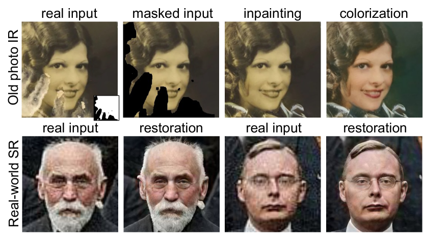
Figure 10: Real-world applications of our method.

​​​​Methods​​​​	​​​​DPS [16]​​​​	​​​​DDRM [36]​​​​	​​​​DDNM [63]​​​​	​​​​Ours-10​​​​	​​​​Ours-15​​​​	​​​​Ours-20​​​​
Time (s)	468.85	5.26	12.67	12.11	16.53	21.19
PSNR↑	21.82	37.69	38.40	38.58	39.25	39.47

Table 4: Running time of different methods. $*$-T: T timesteps.

Methods	ImageNet			CelebaA-HQ
	PSNR↑	​​​​​​​​SSIM↑​​​​​​​​	LPIPS↓	PSNR↑	​​​​​​​​​​SSIM↑​​​​​​​​​​	LPIPS↓
SRGAN [40]	24.83	​​​​​​0.696​​​​​​	0.245	31.16	​​​​​​0.868​​​​​​	0.164
​​​​BSRGAN [78]​​​​	23.65	​​​​​​0.651​​​​​​	0.331	27.80	​​​​​​0.808​​​​​​	0.216
LDM [53]	22.34	​​​​​​0.606​​​​​​	0.318	27.18	​​​​​​0.783​​​​​​	0.208
DiffIR [67]	29.25	​​​​​0.814​​​​​	0.235	34.96	​​​​​0.924​​​​​	0.121
DeqIR (Ours)	27.44	​​​​​0.782​​​​	0.235	32.19	​​​​​0.887​​​​​	0.154

Table 5: Comparisons of supervised learning methods and our zero-shot method on ImageNet for $4\times$ SR.

6 Conclusion

In this paper, we have proposed a novel zero-shot diffusion-based IR method, called DeqIR. Specifically, we model diffusion-based IR generation as a deep equilibrium (DEQ) fixed point system. Our IR method can conduct parallel sampling, instead of long sequential sampling in traditional diffusion models. Based on the DEQ inversion, we are able to explore the relationship between the restoration and initialization. With the initialization optimization, the restoration performance can be improved and the generation direction can be guided with additional information. Extensive experiments demonstrate that our proposed DeqIR achieves better performance on different IR tasks. Moreover, our DeqIR can be generalized to other real-world applications.

References

- Amos and Kolter [2017] Brandon Amos and J Zico Kolter. Optnet: Differentiable optimization as a layer in neural networks. In ICML, 2017.
- Anderson [1965] Donald G Anderson. Iterative procedures for nonlinear integral equations. Journal of the ACM, 1965.
- Bai et al. [2019] Shaojie Bai, J Zico Kolter, and Vladlen Koltun. Deep equilibrium models. NeurIPS, 2019.
- Bai et al. [2020] Shaojie Bai, Vladlen Koltun, and J Zico Kolter. Multiscale deep equilibrium models. NeurIPS, 2020.
- Bai et al. [2022] Shaojie Bai, Zhengyang Geng, Yash Savani, and J Zico Kolter. Deep equilibrium optical flow estimation. In CVPR, 2022.
- Broyden [1965] Charles G Broyden. A class of methods for solving nonlinear simultaneous equations. Mathematics of computation, 1965.
- Cao et al. [2021] Jiezhang Cao, Yawei Li, Kai Zhang, and Luc Van Gool. Video super-resolution transformer. arXiv preprint arXiv:2106.06847, 2021.
- Cao et al. [2022] Jiezhang Cao, Jingyun Liang, Kai Zhang, Yawei Li, Yulun Zhang, Wenguan Wang, and Luc Van Gool. Reference-based image super-resolution with deformable attention transformer. In ECCV, 2022.
- Cao et al. [2023] Jiezhang Cao, Qin Wang, Yongqin Xian, Yawei Li, Bingbing Ni, Zhiming Pi, Kai Zhang, Yulun Zhang, Radu Timofte, and Luc Van Gool. Ciaosr: Continuous implicit attention-in-attention network for arbitrary-scale image super-resolution. In CVPR, 2023.
- Cavigelli et al. [2017] Lukas Cavigelli, Pascal Hager, and Luca Benini. Cas-cnn: A deep convolutional neural network for image compression artifact suppression. In IJCNN, 2017.
- Chen et al. [2021] Hanting Chen, Yunhe Wang, Tianyu Guo, Chang Xu, Yiping Deng, Zhenhua Liu, Siwei Ma, Chunjing Xu, Chao Xu, and Wen Gao. Pre-trained image processing transformer. In CVPR, 2021.
- Chen et al. [2022] Liangyu Chen, Xiaojie Chu, Xiangyu Zhang, and Jian Sun. Simple baselines for image restoration. In ECCV, 2022.
- Chen et al. [2018] Ricky TQ Chen, Yulia Rubanova, Jesse Bettencourt, and David K Duvenaud. Neural ordinary differential equations. NeurIPS, 2018.
- Chen et al. [2023] Xiangyu Chen, Xintao Wang, Jiantao Zhou, Yu Qiao, and Chao Dong. Activating more pixels in image super-resolution transformer. In CVPR, 2023.
- Choi et al. [2021] Jooyoung Choi, Sungwon Kim, Yonghyun Jeong, Youngjune Gwon, and Sungroh Yoon. Ilvr: Conditioning method for denoising diffusion probabilistic models. In ICCV, 2021.
- Chung et al. [2023] Hyungjin Chung, Jeongsol Kim, Michael T Mccann, Marc L Klasky, and Jong Chul Ye. Diffusion posterior sampling for general noisy inverse problems. ICLR, 2023.
- Dai et al. [2019] Tao Dai, Jianrui Cai, Yongbing Zhang, Shu-Tao Xia, and Lei Zhang. Second-order attention network for single image super-resolution. In CVPR, 2019.
- Deng et al. [2009] Jia Deng, Wei Dong, Richard Socher, Li-Jia Li, Kai Li, and Li Fei-Fei. Imagenet: A large-scale hierarchical image database. In CVPR, 2009.
- Dhariwal and Nichol [2021] Prafulla Dhariwal and Alexander Nichol. Diffusion models beat gans on image synthesis. NeurIPS, 2021.
- Djolonga and Krause [2017] Josip Djolonga and Andreas Krause. Differentiable learning of submodular models. NeurIPS, 2017.
- Dong et al. [2015a] Chao Dong, Yubin Deng, Chen Change Loy, and Xiaoou Tang. Compression artifacts reduction by a deep convolutional network. In ICCV, 2015a.
- Dong et al. [2015b] Chao Dong, Chen Change Loy, Kaiming He, and Xiaoou Tang. Image super-resolution using deep convolutional networks. TPAMI, 2015b.
- Donti et al. [2021] Priya L Donti, David Rolnick, and J Zico Kolter. Dc3: A learning method for optimization with hard constraints. arXiv preprint arXiv:2104.12225, 2021.
- Dupont et al. [2019] Emilien Dupont, Arnaud Doucet, and Yee Whye Teh. Augmented neural odes. NeurIPS, 2019.
- Fu et al. [2019] Xueyang Fu, Zheng-Jun Zha, Feng Wu, Xinghao Ding, and John Paisley. Jpeg artifacts reduction via deep convolutional sparse coding. In ICCV, 2019.
- Fu et al. [2021] Xueyang Fu, Menglu Wang, Xiangyong Cao, Xinghao Ding, and Zheng-Jun Zha. A model-driven deep unfolding method for jpeg artifacts removal. TNNLS, 2021.
- Fung et al. [2021] Samy Wu Fung, Howard Heaton, Qiuwei Li, Daniel McKenzie, Stanley Osher, and Wotao Yin. Fixed point networks: Implicit depth models with jacobian-free backprop. arXiv preprint arXiv:2103.12803, 2021.
- Geng et al. [2020] Zhengyang Geng, Meng-Hao Guo, Hongxu Chen, Xia Li, Ke Wei, and Zhouchen Lin. Is attention better than matrix decomposition? In ICLR, 2020.
- Geng et al. [2021] Zhengyang Geng, Xin-Yu Zhang, Shaojie Bai, Yisen Wang, and Zhouchen Lin. On training implicit models. NeurIPS, 2021.
- Gu et al. [2021] Albert Gu, Karan Goel, and Christopher Ré. Efficiently modeling long sequences with structured state spaces. arXiv preprint arXiv:2111.00396, 2021.
- Gu et al. [2020] Fangda Gu, Heng Chang, Wenwu Zhu, Somayeh Sojoudi, and Laurent El Ghaoui. Implicit graph neural networks. NeurIPS, 2020.
- Gulrajani et al. [2017] Ishaan Gulrajani, Faruk Ahmed, Martin Arjovsky, Vincent Dumoulin, and Aaron Courville. Improved training of wasserstein gans. arXiv preprint arXiv:1704.00028, 2017.
- Ho et al. [2020] Jonathan Ho, Ajay Jain, and Pieter Abbeel. Denoising diffusion probabilistic models. NeurIPS, 2020.
- Jia et al. [2019] Xixi Jia, Sanyang Liu, Xiangchu Feng, and Lei Zhang. Focnet: A fractional optimal control network for image denoising. In CVPR, 2019.
- Karras et al. [2018] Tero Karras, Timo Aila, Samuli Laine, and Jaakko Lehtinen. Progressive growing of GANs for improved quality, stability, and variation. In ICLR, 2018.
- Kawar et al. [2022] Bahjat Kawar, Michael Elad, Stefano Ermon, and Jiaming Song. Denoising diffusion restoration models. NeurIPS, 2022.
- Kim et al. [2016] Jiwon Kim, Jung Kwon Lee, and Kyoung Mu Lee. Accurate image super-resolution using very deep convolutional networks. In CVPR, 2016.
- Kim et al. [2019] Yoonsik Kim, Jae Woong Soh, Jaewoo Park, Byeongyong Ahn, Hyun-Seung Lee, Young-Su Moon, and Nam Ik Cho. A pseudo-blind convolutional neural network for the reduction of compression artifacts. TCSVT, 2019.
- Kingma et al. [2021] Diederik Kingma, Tim Salimans, Ben Poole, and Jonathan Ho. Variational diffusion models. NeurIPS, 2021.
- Ledig et al. [2017] Christian Ledig, Lucas Theis, Ferenc Huszár, Jose Caballero, Andrew Cunningham, Alejandro Acosta, Andrew Aitken, Alykhan Tejani, Johannes Totz, Zehan Wang, et al. Photo-realistic single image super-resolution using a generative adversarial network. In CVPR, 2017.
- Li et al. [2022a] Mingjie Li, Yisen Wang, and Zhouchen Lin. Cerdeq: Certifiable deep equilibrium model. In ICML, 2022a.
- Li et al. [2022b] Wenbo Li, Zhe Lin, Kun Zhou, Lu Qi, Yi Wang, and Jiaya Jia. Mat: Mask-aware transformer for large hole image inpainting. In CVPR, 2022b.
- Liang et al. [2021] Jingyun Liang, Jiezhang Cao, Guolei Sun, Kai Zhang, Luc Van Gool, and Radu Timofte. Swinir: Image restoration using swin transformer. In ICCVW, 2021.
- Liang et al. [2022] Jingyun Liang, Jiezhang Cao, Yuchen Fan, Kai Zhang, Rakesh Ranjan, Yawei Li, Radu Timofte, and Luc Van Gool. Vrt: A video restoration transformer. arXiv preprint arXiv:2201.12288, 2022.
- Lin et al. [2023] Xinqi Lin, Jingwen He, Ziyan Chen, Zhaoyang Lyu, Ben Fei, Bo Dai, Wanli Ouyang, Yu Qiao, and Chao Dong. Diffbir: Towards blind image restoration with generative diffusion prior. arXiv preprint arXiv:2308.15070, 2023.
- Lu et al. [2021] Cheng Lu, Jianfei Chen, Chongxuan Li, Qiuhao Wang, and Jun Zhu. Implicit normalizing flows. In ICLR, 2021.
- Lu et al. [2022] Cheng Lu, Yuhao Zhou, Fan Bao, Jianfei Chen, Chongxuan Li, and Jun Zhu. Dpm-solver: A fast ode solver for diffusion probabilistic model sampling in around 10 steps. NeurIPS, 35:5775–5787, 2022.
- Lugmayr et al. [2022] Andreas Lugmayr, Martin Danelljan, Andres Romero, Fisher Yu, Radu Timofte, and Luc Van Gool. Repaint: Inpainting using denoising diffusion probabilistic models. In CVPR, 2022.
- Menon et al. [2020] Sachit Menon, Alexandru Damian, Shijia Hu, Nikhil Ravi, and Cynthia Rudin. Pulse: Self-supervised photo upsampling via latent space exploration of generative models. In CVPR, 2020.
- Pan et al. [2021] Xingang Pan, Xiaohang Zhan, Bo Dai, Dahua Lin, Chen Change Loy, and Ping Luo. Exploiting deep generative prior for versatile image restoration and manipulation. TPAMI, 2021.
- Pathak et al. [2016] Deepak Pathak, Philipp Krahenbuhl, Jeff Donahue, Trevor Darrell, and Alexei A Efros. Context encoders: Feature learning by inpainting. In CVPR, 2016.
- Pokle et al. [2022] Ashwini Pokle, Zhengyang Geng, and J Zico Kolter. Deep equilibrium approaches to diffusion models. NeurIPS, 2022.
- Rombach et al. [2022] Robin Rombach, Andreas Blattmann, Dominik Lorenz, Patrick Esser, and Björn Ommer. High-resolution image synthesis with latent diffusion models. In CVPR, 2022.
- Saharia et al. [2022a] Chitwan Saharia, William Chan, Huiwen Chang, Chris Lee, Jonathan Ho, Tim Salimans, David Fleet, and Mohammad Norouzi. Palette: Image-to-image diffusion models. In ACM SIGGRAPH, 2022a.
- Saharia et al. [2022b] Chitwan Saharia, Jonathan Ho, William Chan, Tim Salimans, David J Fleet, and Mohammad Norouzi. Image super-resolution via iterative refinement. TPAMI, 2022b.
- Song et al. [2021a] Jiaming Song, Chenlin Meng, and Stefano Ermon. Denoising diffusion implicit models. ICLR, 2021a.
- Song et al. [2021b] Yang Song, Jascha Sohl-Dickstein, Diederik P Kingma, Abhishek Kumar, Stefano Ermon, and Ben Poole. Score-based generative modeling through stochastic differential equations. ICLR, 2021b.
- Wang et al. [2023a] Jianyi Wang, Zongsheng Yue, Shangchen Zhou, Kelvin CK Chan, and Chen Change Loy. Exploiting diffusion prior for real-world image super-resolution. In arXiv preprint arXiv:2305.07015, 2023a.
- Wang et al. [2023b] Shuai Wang, Yao Teng, and Limin Wang. Deep equilibrium object detection. In ICCV, 2023b.
- Wang et al. [2020] Tiancai Wang, Xiangyu Zhang, and Jian Sun. Implicit feature pyramid network for object detection. arXiv preprint arXiv:2012.13563, 2020.
- Wang et al. [2018] Xintao Wang, Ke Yu, Shixiang Wu, Jinjin Gu, Yihao Liu, Chao Dong, Yu Qiao, and Chen Change Loy. Esrgan: Enhanced super-resolution generative adversarial networks. In ECCVW, 2018.
- Wang et al. [2021] Xintao Wang, Liangbin Xie, Chao Dong, and Ying Shan. Real-esrgan: Training real-world blind super-resolution with pure synthetic data. In ICCVW, 2021.
- Wang et al. [2023c] Yinhuai Wang, Jiwen Yu, and Jian Zhang. Zero-shot image restoration using denoising diffusion null-space model. ICLR, 2023c.
- Wei and Kolter [2021] Colin Wei and J Zico Kolter. Certified robustness for deep equilibrium models via interval bound propagation. In ICLR, 2021.
- Whang et al. [2022] Jay Whang, Mauricio Delbracio, Hossein Talebi, Chitwan Saharia, Alexandros G Dimakis, and Peyman Milanfar. Deblurring via stochastic refinement. In CVPR, 2022.
- Xia et al. [2022] Bin Xia, Yucheng Hang, Yapeng Tian, Wenming Yang, Qingmin Liao, and Jie Zhou. Efficient non-local contrastive attention for image super-resolution. AAAI, 2022.
- Xia et al. [2023a] Bin Xia, Yulun Zhang, Shiyin Wang, Yitong Wang, Xinglong Wu, Yapeng Tian, Wenming Yang, and Luc Van Gool. Diffir: Efficient diffusion model for image restoration. In ICCV, 2023a.
- Xia et al. [2023b] Bin Xia, Yulun Zhang, Yitong Wang, Yapeng Tian, Wenming Yang, Radu Timofte, and Luc Van Gool. Knowledge distillation based degradation estimation for blind super-resolution. ICLR, 2023b.
- Xie et al. [2019] Chaohao Xie, Shaohui Liu, Chao Li, Ming-Ming Cheng, Wangmeng Zuo, Xiao Liu, Shilei Wen, and Errui Ding. Image inpainting with learnable bidirectional attention maps. In ICCV, 2019.
- Yang et al. [2022] Zonghan Yang, Tianyu Pang, and Yang Liu. A closer look at the adversarial robustness of deep equilibrium models. NeurIPS, 2022.
- Yi et al. [2020] Zili Yi, Qiang Tang, Shekoofeh Azizi, Daesik Jang, and Zhan Xu. Contextual residual aggregation for ultra high-resolution image inpainting. In CVPR, 2020.
- Yu et al. [2018] Jiahui Yu, Zhe Lin, Jimei Yang, Xiaohui Shen, Xin Lu, and Thomas S Huang. Generative image inpainting with contextual attention. In CVPR, 2018.
- Yu et al. [2019] Jiahui Yu, Zhe Lin, Jimei Yang, Xiaohui Shen, Xin Lu, and Thomas S Huang. Free-form image inpainting with gated convolution. In ICCV, 2019.
- Yue and Loy [2022] Zongsheng Yue and Chen Change Loy. Difface: Blind face restoration with diffused error contraction. arXiv preprint arXiv:2212.06512, 2022.
- Zamir et al. [2022] Syed Waqas Zamir, Aditya Arora, Salman Khan, Munawar Hayat, Fahad Shahbaz Khan, and Ming-Hsuan Yang. Restormer: Efficient transformer for high-resolution image restoration. In CVPR, 2022.
- Zeng et al. [2022] Yanhong Zeng, Jianlong Fu, Hongyang Chao, and Baining Guo. Aggregated contextual transformations for high-resolution image inpainting. TVCG, 2022.
- Zhang et al. [2021a] Kai Zhang, Yawei Li, Wangmeng Zuo, Lei Zhang, Luc Van Gool, and Radu Timofte. Plug-and-play image restoration with deep denoiser prior. TPAMI, 2021a.
- Zhang et al. [2021b] Kai Zhang, Jingyun Liang, Luc Van Gool, and Radu Timofte. Designing a practical degradation model for deep blind image super-resolution. In ICCV, 2021b.
- Zhang et al. [2018] Yulun Zhang, Kunpeng Li, Kai Li, Lichen Wang, Bineng Zhong, and Yun Fu. Image super-resolution using very deep residual channel attention networks. In ECCV, 2018.
- Zhu et al. [2023] Yuanzhi Zhu, Kai Zhang, Jingyun Liang, Jiezhang Cao, Bihan Wen, Radu Timofte, and Luc Van Gool. Denoising diffusion models for plug-and-play image restoration. In CVPRW, 2023.