Hadronic Vacuum Polarization Contribution to
as a function of the external lepton mass
Abstract
The hadronic vacuum polarization contribution to the anomalous magnetic moment of a lepton is considered as a function of the lepton mass. We show how the analyticity properties of this function allow for its full reconstruction when it is only known in a restricted mass region. Assuming that LQCD could evaluate it in an optimal mass region we show, within the framework of a phenomenological model, how to reconstruct the function elsewhere, in particular at the muon mass value.
1 Introduction
The result obtained by The Muon g-2 Collaboration at Fermilab Fermilab23 :
| (1) |
when combined with previous measurements brings the present experimental world average
| (2) |
to the remarkable level of a ppm precision. This has to be contrasted with the theoretical evaluation of which, at present, is not competitive at the same level of precision because of discrepancies in the evaluation of the hadronic vacuum polarization (HVP) contribution.
All data driven determinations of the HVP contribution to the anomalous magnetic moment of the muon (anomaly for short) have so far been made using the dispersive representation BM61 ; BdeR68 ; Gourdin:1969dm :
| (3) |
where denotes the spectral function of hadronic vacuum polarization, related by the optical theorem to the one-photon annihilation cross-section
| (4) |
that is obtained from experiments Davier , Teubner . The results however, at the level of the desired accuracy, disagree significantly with the lattice QCD evaluation reported in ref. BMW21 , subsequently confirmed at least partially in L1 ; L2 ; L3 ; L4 . 111There is also a disagreement between the results of Davier , Teubner and a more recent result CMD3 . A recent detailed discussion of all these evaluations can be found in Davieretal23 ; Benton:2023fcv .
Here we shall focus our attention on the HVP evaluation of the anomaly when the mass of the external lepton has an arbitrary value , more precisely on the evaluation of the anomaly in terms of the ratio
| (5) |
where denotes the external lepton mass and the fixed hadronic threshold. Our aim is to reconstruct the dependence of the anomaly in a large -domain, covering in particular the muon value, from its knowledge in a restricted -region. This may be of interest in the case where one could obtain from LQCD simulations accurate determinations of the anomaly in a given optimal -region. There is no problem in evaluating the anomaly from data at any desired -value, which offers the possibility of comparing the data -shape to the LQCD -shape, thus providing a new way of investigating the origin of the HVP discrepancies.
The paper is organized as follows. The HVP anomaly function for an arbitrary lepton mass is introduced in the next section with special attention to its asymptotic behaviour properties. The content of the so called transfer theorem of Flajolet and Odlyzko FO90 ; FS09 (FO-theorem for short) and its application in implementing reconstruction approximants to the anomaly function is discussed in Section 3. An illustration of this reconstruction procedure is discussed in Section 4 within the framework of a phenomenological model of the hadronic spectral function. This provides a simulation on how the reconstruction procedure could be applied to LQCD data.
The conclusions are in Section 5.
2 The HVP Anomaly Function
It is convenient, for our purposes, to use the Mellin-Barnes representation of the anomaly proposed in ref. EdeR14
| (6) |
where the function denotes the Mellin transform of the kernel in Eq. (3)
| (7) |
and is the Mellin transform of the spectral function of hadronic vacuum polarization
| (8) |
In this representation the -domain of integration in Eq. (6) can then be extended to the full complex -plane by analytic continuation .
Moments of the hadronic spectral function correspond to negative integer -values of :
| (9) |
They are accessible to experiment and also, in principle, to LQCD because they are related deR17 to derivatives of the HVP self-energy function in the Euclidean at
| (10) |
More generally, the Mellin transform is a meromorphic function with poles in the real -axis at . Under the assumption that all the poles are simple, has then a singular expansion FGD94 of the type:
| (11) |
with the residue of the pole at .
The function can be used as a gauge of the underlying HVP structure. For example, at the leading contribution is given by the residue of the pole at in the integrand of Eq. (6) with the result BdeR69 :
| (12) |
This contribution is governed by the long-distance behaviour of HVP expressed here, either in terms of the moment of the spectral function accessible to experiment, or in terms of the slope of the HVP self-energy function at the euclidean origin accessible to LQCD (see e.g. ref. BMW17 ). In the case where this asymptotic contribution practically amounts to a calculation of the electron anomaly.
On the other hand, at , the leading contribution is given by the residue of the double pole at in the integrand of Eq. (6) with the result
| (13) |
that follows from the familiar short-distance leading behaviour of HVP in QCD. In the case where it dominates the HVP contribution to the -anomaly.
We want to study the shape of the function in between these two extreme regimes. We shall do that using the technique of reconstruction approximants that follow from the FO-theorem FO90 ; FS09 , i.e. the same technique that has been used in our previous work in refs. GdeR22 ; GdeR23 . The aim here is to reconstruct the function in its full -domain when one knows it accurately, e.g. from LQCD simulations, in an optimal -region. Not surprisingly, this reconstruction depends crucially on the details of the analytic properties of the function that we next review.
2.1 Asymptotic Behaviours of
The asymptotic behaviour of for , which includes the cases of the muon and electron in particular, is governed by the singular expansion of the -integrand in Eq. (6) at the left of the fundamental strip FGD94 , i.e. the region where
| (14) |
The are the residues of the singularities at with multiplicities and generated by the function ( is not singular in the region ). The resulting asymptotic expansion of the function has then the form
| (15) | |||||
| (16) |
where e.g.
| (17) |
Observe that this series has non-analytic terms of the type , induced by the double poles of the function in Eq. (7) at .
On the other hand the asymptotic expansion of when , which applies in particular to the of the -lepton, is governed by the singularities of at the right of the fundamental strip in Eq. (6), i.e. the region where
| (18) |
with the residues of the singularities at with multiplicity generated by the product of the singularities of and . The resulting asymptotic expansion of in this case, which also has non-analytic terms, is slightly more complicated:
| (19) | ||||
| (20) |
where in particular
| (21) |
The non-analytic terms that appear in the expansions of , both at and at , are the basic ingredients of the reconstruction approximants of the full function that we next discuss.
3 The FO-theorem and Reconstruction Approximants
The FO-theorem FO90 ; FS09 relates the non-analyticity of a function defined in a finite domain to the large order behaviour of the coefficients of its Taylor expansion in its analyticity domain. In order to apply this theorem to the function we first perform a mapping of the infinite domain onto a finite -domain via the conformal transformation:
| (22) |
which maps the -domain to the unit disc and in particular:
| (23) |
The content of the FO-theorem is then encoded in the identity:
| (24) |
where the denote the coefficients of the Taylor expansion of at (the image of where is analytic). The are the coefficients of the same Taylor series as and the FO-theorem relates them to the non-analyticity of the function (in our case at and at , the images of and ) in a precise way. The third term in the r.h.s. of Eq. (24) is then the singular function that emerges from the resulting power series sums.
When (the image of ) the anomaly function has a Taylor series expansion in -powers
| (25) |
with coefficients:
| (26) |
and
| (27) |
where
| (28) |
The coefficients and for are accessible to experiment by measuring the hadronic integrals above. In principle they are also accessible to LQCD from a fit to evaluations of the anomaly function in the region of small -values (i.e. around ), though this will not be required in the reconstruction procedure that we shall propose. It could be of interest, however, if the optimal region for a LQCD evaluation happens to be in the -analyticity domain.
We are now in the position to specify the precise way that the FO-theorem relates the coefficients to the non-analiticity of the function at () and at ().
3.1 Reconstruction Approximants
Let us consider the leading non-analytic contributions in Eqs. (15) and (2.1). When expressed in terms of the -variable they become
| (29) |
and
| (30) |
The FO-theorem relates them to the large- behaviour of the coefficients as follows: 222The mappings for arbitrary types of singular terms in asymptotic expansions are discussed in the Appendices of refs. GdeR22 , GdeR23 and more generally in ref. FS09 .
| (31) |
and
| (32) |
The singular functions induced by these coefficients are then:
| (33) |
and
| (34) |
Therefore, at the leading order that we are considering, the singular function in Eq. (24) becomes:
| (35) |
and the underlined coefficients in Eq. (24) are
| (36) |
Reconstruction approximants to the anomaly function are then obtained by restricting the -polynomial in Eq. (24) to a finite number of terms:
| (37) |
The contribution of the polynomial in the r.h.s. can in fact be further improved if expressed in terms of rational approximants 333See for example ref. CV23 and references therein. Notice that rational approximants like are different to Padé approximants. They don’t require convergence order by order in ( and ) and they don’t need the requirement of Stieltjes behaviour of the function . The motivation to introduce them here is based on the content of the FO theorem which implies that in order to fix all the coefficients one also needs to know all the associated singular functions. The rational approximants to the truncated polynomials provides a way to implement physical requirements that a limited number of singular functions cannot fully reproduce.:
| (38) |
with the coefficients and fixed by the following requirements:
-
•
The coefficients of the Taylor expansion of at must coincide with those of the polynomial, which implies
(39) -
•
The and coefficients are furthermore restricted by the physical requirement that at (i.e. at )
(40) and
(41) This fixes the coefficients and in terms of the other parameters.
-
•
With the coefficients and fixed the way described above, the final form of the reconstruction approximants that we shall consider are then
(42) with given in Eq. (35).
In the next section we shall first check how these reconstruction approximants work in the case of a simple phenomenological model of the hadronic spectral function. Encouraged by the results obtained we shall then discuss how to apply them to LQCD evaluations.
4 Illustration with a Phenomenological Model
The spectral function of the simple model that we shall consider is inspired from PT and phenomenology 444It is a simplified version of phenomenological spectral functions discussed in the literature, see e.g. ref. CHK21 and references therein.:
| (43) |
It has a Breit-Wigner–like modulous squared form factor
| (44) |
with an energy dependent width:
| (45) |
plus a function
| (46) |
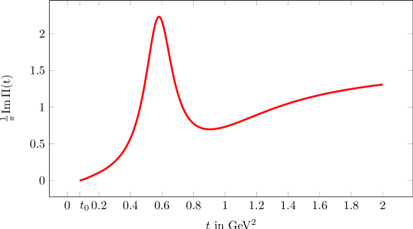
with two arbitrary parameters and . This function has been added so as to smoothly match the low energy phenomenological spectrum of the model to the pQCD asymptotic continuum generated by the sum of quark flavors. The shape of this spectral function, using the physical central values for , , , , and the choice , , with , is shown in Fig (1).
4.1 Reconstruction of the Anomaly Function
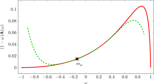
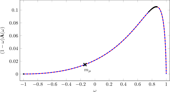
The shape of the anomaly function that follows from this phenomenological model, modulated by a convenient factor that makes it finite everywhere, is shown in Fig. (2) (the red curve). The Taylor series in Eq. (25) with the model coefficients and evaluated as in Eqs. (26) and (27) reproduces rather well, with a few terms, the model function in the region . It quickly fails, however, outside this window. As an example, the dashed green curve shows the shape of the Taylor series with seven terms.
The reconstruction approximants improve considerably the Taylor series results. With terms in the polynomial, and the choice of the rational improvement in Eq. (38), the resulting reconstruction approximant satisfying the restrictions in Eqs. (40) and (41) is then
| (47) |
with
| (48) | |||||
| (49) |
The values of the parameters of this approximant, fixed by the model are:
| (50) |
and
| (51) |
| (52) |
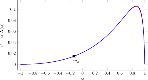
This reconstruction approximant reproduces very well, as shown in Fig. (3), the full -shape of the model function : the blue curve of the reconstruction approximant practically overlaps the red curve of the model function ; in particular, the value of the anomaly at the physical -point is reproduced at the level of the number of digits retained in the plots.
4.2 Reconstruction from a simulation of LQCD Data
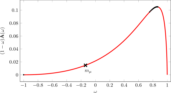
We shall now discuss how to implement reconstruction approximants in the case where LQCD could provide -data points in an optimal region. To be precise, we assume that the optimal region is at rather large values of the lepton mass 555This has been suggested to us by Laurent Lellouch.. We choose the data that simulates potential LQCD data to be provided by the values of the model function at 15 points equally spaced in the interval (i.e. for a lepton mass of to ); this is shown in Figure (4) . We then fit this data to the coefficients and of the function in Eq. (42) with the constraints given by Eqs. (48) and (49) and the coefficients and fixed by the model (recall that in QCD and are given by the short-distance behaviour of HVP in Eq. (13) and the slope of the HVP self-energy function at the origin in Eq. (12)). The resulting approximant is the dashed blue curve in Fig. (5) which reproduces quite well the shape of the model function; in particular the value of the muon anomaly is reproduced at the level.
5 Conclusions
The function which gives the HVP contribution to the of a lepton in terms of its mass may be a way, via LQCD simulations, to obtain the theoretical value of the contribution to the muon anomaly. We have shown that the analyticity properties of its functional dependence on the lepton mass provides a way to reconstruct the full function, in particular at the muon mass value, when one knows its shape in an optimal region of mass values. Within the example of a phenomenological model of the hadronic spectral function, we have shown how to implement this reconstruction in the case where the optimal region of lepton masses lies between and . The results are very encouraging.
References
- (1) D.P. Aguillard et al., Phys. Rev. Lett., 131 161802 (2023).
- (2) C. Bouchiat and L. Michel, J. Phys. Radium 22 121 (1961).
- (3) S.J. Brodsky and E. de Rafael, Phys. Rev. 168 1620 (1968).
- (4) M. Gourdin and E. de Rafael, Nucl. Phys. B 10 (1969), 667-674.
- (5) M. Davier, A. Hoecker, B. Malaescu and Z. Zhang, Eur.Phys.J C 80 241 (2020), [Erratum: Eur.Phys.J. C 80 410 (2020)].
- (6) A. Keshavarzi, D. Nomura and T. Teubner, Phys. Rev. D101 014029 (2020).
- (7) F.V. Ignatov et al. (CMD-3) arXiv:2302.08834[hep-ex].
- (8) S. Borsanyi et al., Nature 593, 51 (2021), arXiv:2002.12347 [hep-lat].
- (9) M. C‘e et al., Phys. Rev. D 106, 114502 (2022), arXiv:2206.06582 [hep-lat].
- (10) C. Alexandrou et al., (Extended Twisted Mass), Phys. Rev. D 107, 074506 (2023), arXiv:2206.15084 [hep-lat].
- (11) T. Blum et al., (2023), arXiv:2301.08696 [hep-lat].
- (12) A. Bazavov et al., (2023), arXiv:2301.08274 [hep-lat].
- (13) M. Davier et al., arXiv:2308.04221v1 [hep-ph].
- (14) G. Benton et al., arXiv:2311.09523 [hep-ph].
- (15) Ph. Flajolet and A. Odlyzko, SIAM J. Discrete Math. 3 216 (1990).
- (16) Philippe Flajolet and Robert Sedgewick, Analytic Combinatorics, Cambridge University Press, 2009.
- (17) E. de Rafael, Phys. Lett. B736 52 (2014).
- (18) E. de Rafael, Phys. Rev. D96, 014510 (2017).
- (19) Ph. Flajolet, X. Gourdon and Ph. Dumas, Theor. Comput. Sci. 144 3 (1994).
- (20) J.S. Bell and E. de Rafael, Nucl. Phys. B11, 611 (1969).
- (21) Sz. Borsany et al, Phys. Rev. D96, 074507 (2017).
- (22) D. Greynat and E. de Rafael, JHEP 05 084 (2022).
- (23) D. Greynat and E. de Rafael, JHEP 03 248 (2023).
- (24) J. Chok and G.M. Vasil, arXiv:2310.12053v1 [math.NA] (2023)
- (25) G. Colangelo, et al. Phys. Lett. B825 136852 (2022).