SeaDSC: A video-based unsupervised method for dynamic scene change detection in unmanned surface vehicles

Abstract

Recently, there has been an upsurge in the research on maritime vision, where a lot of works are influenced by the application of computer vision for Unmanned Surface Vehicles (USVs). Various sensor modalities such as camera, radar, and lidar have been used to perform tasks such as object detection, segmentation, object tracking, and motion planning. A large subset of this research is focused on the video analysis, since most of the current vessel fleets contain the camera’s onboard for various surveillance tasks. Due to the vast abundance of the video data, video scene change detection is an initial and crucial stage for scene understanding of USVs. This paper outlines our approach to detect dynamic scene changes in USVs. To the best of our understanding, this work represents the first investigation of scene change detection in the maritime vision application. Our objective is to identify significant changes in the dynamic scenes of maritime video data, particularly those scenes that exhibit a high degree of resemblance. In our system for dynamic scene change detection, we propose completely unsupervised learning method. In contrast to earlier studies, we utilize a modified cutting-edge generative picture model called VQ-VAE-2 to train on multiple marine datasets, aiming to enhance the feature extraction. Next, we introduce our innovative similarity scoring technique for directly calculating the level of similarity in a sequence of consecutive frames by utilizing grid calculation on retrieved features. The experiments were conducted using a nautical video dataset called RoboWhaler to showcase the efficient performance of our technique.

1 Introduction

Approximately 80% of global trade is conducted through maritime transportation [14]. As the use of sea based transport continues to rise, there is a corresponding increase in incidents such as pirate attacks, trafficking of illegal substances, illegal immigration and fishing, terrorist attacks in port areas, and collisions between marine vehicles, particularly in inland waters, coastal shipping and near the ports. To tackle these challenges, numerous studies have introduced the application of machine learning and deep learning to address various computer vision problems. Extensive research has been conducted on the application of computer vision in USVs to advance the development of autonomous shipping and vessel systems. Equipped with advanced multimodal sensors such as cameras, radar, and lidar etc., much research has been conducted on various computer vision tasks to assure the practical implementation of USVs in real-world scenarios. Several recent literature reviews have provided a systematic overview of various techniques and algorithms used in maritime computer vision. These include maritime object detection, object tracking, segmentation [22, 28], deep learning for maritime vision [18, 17], and comprehensive state-of-the-art (SOTA) maritime datasets for maritime perception [26]. With the increasing expansion of video data collected for marine vision, the significance of video analysis, indexing, browsing, summarization, compression, and retrieval systems has grown considerably [6, 10]. The identification of scene changes in videos is the initial and crucial stage in applications related to visual information retrieval and scene understanding. Nevertheless, this research issue in the field of maritime remains uncommon. In this paper, we present our method for dynamic scene change detection for USVs. To the best of our knowledge, this study represents the inaugural investigation of this problem into the application of maritime vision. Our objective is to identify significant changes in the dynamic scenes of maritime video data, particularly those scenes that exhibit a high degree of resemblance. Determining dynamic scene change on the maritime video will bring many benefits such that help to categorize the potential meaningful action, remove amount of redundant and unnecessary scenes or frames in the future. In this regard, the previous works can be categorized into either a supervised learning strategy or an unsupervised learning technique. Supervised learning methods [15, 7, 8, 9, 5] typically necessitate a substantial amount of data annotation for a preset set of dynamic scenes. These methods then proceed to train a model to identify dynamic scenes in videos. However, data annotation is consistently expensive, and in the emerging field of maritime vision, annotation for this specific purpose is currently unavailable. On the other side, the unsupervised learning approach does not necessitate annotation for training the model. Alternatively, the methodologies described in [23, 19, 4, 20, 25] utilize a representative method that calculates the similarity between every consecutive frame in a video. This calculation is based on low-level features retrieved from the frames, such as color, histogram, gradient, and so on. At a later step, an aggregation algorithm combines all the obtained scores to determine the degree of similarity in scene changes. However, this method could result in inaccuracies since the low-level features may not include sufficient information and may contain noise. In addition, doing calculations on every pair of successive frames in the video segment results in a significant increase in the computational cost. Our novel approach aims to optimize the computational cost while simultaneously improving the accuracy of scene change detection for maritime applications. Initially, we utilize a recent SOTA generative deep learning model, to construct a feature extraction method that improves low-level features beyond what traditional feature extraction can do. Here, we utilize the VQ-VAE-2 model as a basis and make a minor modifications for more lightweight. We then train our model using a collection of maritime datasets in a reconstruction task, without the need for any annotations. During the inference stage, we calculate the similarity magnitude for each sliding window of the video by projecting the features onto the skipped frames of the window. In addition, we calculate the similarity score for a pair of skipping frames using cell calculation of a grid feature. This approach helps to reduce computational cost while maintaining high accuracy in the inference process.

Our main contributions are summarized below:

• We introduce our framework for detecting dynamic scene changes in a video sequence captured by USVs. Our approach utilizes successive frames and relies on unsupervised learning.

• We adapt a SOTA image generating VQ-VAE-2 model [21] to train it on a marine dataset in order to extract sophisticated embedding features.

• As the heart of the component, we propose a novel feature extraction-based scheme for calculating the convulsion score of a segment on its own.

• We use multiple raw datasets in maritime computer vision to demonstrate the effectiveness of our approach and promising performance.

In the following sections, we present existing work in Section 2, then we discuss in the detail of our methodology on the Section 3, and show the results of our experiment on the Section 4. Finally, the Section 5 conclude our works.

2 Related works

2.1 Maritime vision studies

The field of maritime vision has been extensively researched. Several literature reviews have methodically and fully compiled and presented the most recent studies in this field. Qiao Qiao et al. [18, 17] introduced an extensive deep learning approach for the application of USVs in maritime environments. A comprehensive approach utilizing deep learning is proposed to address the challenges associated with USVs. This approach encompasses several tasks and methodologies including environment perception, state estimation, and path planning. These tasks are effectively tackled through the application of supervised, unsupervised, and reinforcement learning methods. Zhang et al. [28] conducted a thorough investigation and extensive comparison of object detection approaches, with a particular emphasis on the maritime domain. Their study specifically examined deep learning models, including CNN-based methods and YOLO-based methods, from 2012 to 2021. Iwin et al. [22] conducted a comprehensive analysis of the existing research on deep learning techniques for ship object detection and recognition. In addition to the literature studies on USVs approaches, a literature study is also being undertaken on maritime vision datasets. Su et al. [26] provided a comprehensive overview of publicly available maritime datasets for the purpose of maritime perception. A total of 15 state-of-the-art public datasets are systematically presented, which consist of multi-modal sensors including cameras, lidar, and radar sensors for data collecting.

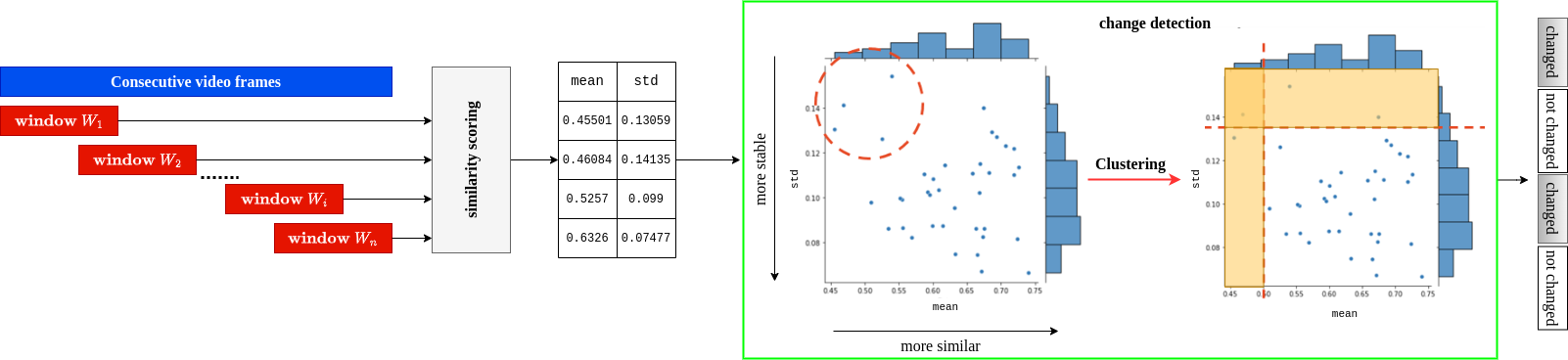
Figure 1: Our proposed SeaDSC framework for scene change detection for USVs.

2.2 Scene change detection methods

Kowdle et al. [12] introduced a technique for detecting dynamic scene changes in videos, which can be applied to video analysis tasks like video summarization. The method suggests a computational approach for determining the similarity between each pair of frames within a sliding window. This study evaluated the model’s performance on the movie dataset [2] using precision, recall, and F1-score measures. This work calculates the similarity between consecutive pairs of frames in a sliding window, which results in increased processing costs. Furthermore, the utilization of optical flow in the method results in features that are of low quality, imprecise, and affected by noise. Salih et al. [23] present a technique for detecting dynamic scene changes in video coding. The main objective in this context is to achieve video compression by removing the temporal redundancy between consecutive frames. The four matching methods available are: Absolute Frame Difference (AFD), Mean Absolute Frame Differences (MAFD), Mean Histogram Absolute Frame Difference (MHAFD), and Maximum Gradient Value (MGV). However, the method mainly depended on handcrafted features such as color, histogram, or image gradient, which are still limited and may contain a significant amount of noise. Furthermore, the calculation of each successive pair of frames incurs a significant computational expense. Rascioni et al. [19] introduced their technique for detecting dynamic scene changes in H264 encoded video. This study measure dissimilarity by analyzing different features, including pixel-level comparison, global histogram, block-based histogram, and motion-based histogram of video sequences. The objective is to detect scene changes in movies. The method primarily depended on domain-specific information for feature extraction and threshold determination, resulting in inaccuracies and unreliability for real-world applications. Peng et al. [15] proposed a method for dynamic scene identification using a sequence model called LSTM. This model aggregates the trajectory of information retrieved from CNNs to categorize scenes. Feichtenhofer et al. [7, 8] introduced a method for dynamic scene detection. They utilized a feature extraction process that specifically targeted spatial and spatiotemporal information to identify dynamic scenes in subsequent stages. The proposed model relies on the ResNet backbone and requires annotated data for training, which may not always be available in various domains. Aalok et al. [9] presented a technique for extracting features from Convolutional Neural Networks (CNNs). These features are then combined into a high-dimensional vector and fed into a Support Vector Machine (SVM) classifier to determine the dynamic scene. However, this strategy also necessitates a substantial amount of annotated data in order to train the model. Liang et al. [5] present a system with multiple stages to train an algorithm for detecting scene changes in videos. Dorfeshan et al. [4] presented a technique for detecting dynamic scene changes by calculating the similarity between video frames’ histograms. Rayatifard et al. [20] addressed the problem of dynamic scene recognition for video segmentation. They specifically focus on HEVC/H.265 video streams, where the similarity between consecutive frames is computed using the compressed bitstream signal. This similarity is then used to identify scene changes. Shukla et al. [25] introduced their method for detecting scene changes in videos. Their approach involves using histograms, binary search, and linear interpolation to filter out comparable frames in the video.

The regular metric for evaluating a (dynamic) scene change detection are recall, precision, and F1-score as all above studies for scene change detection.

3 Method

Our goal is to determine whether a changed part of a video has been presented. The target scene has changed significantly and continuously over a long period of time. A static scene, on the other hand, is one that remains motionless or unchanged for an extended period of time. For example, USVs typically travel in a straight line along the beach for extended periods of time without encountering other USVs or changing their surroundings. Other instances where the camera is obstructed or another USV blocks the ego USV for an extended period of time could be considered unchanged scenes.

The framework we propose is seen in Figure 1. Within our architecture, we initially partition a given video into windows of equal duration. By utilizing a stride that is less than the length of the window, it is possible to overlap the window. Subsequently, each window is subjected to a similarity scoring method in order to determine the degree of similarity inside that window. A higher score, in essence, indicates that the entire frame in the video has a similarity to each other, implying that this window could be considered a potential instance of no scene change. The similarity scoring module will generate the mean and standard deviation of the similarity score, which is used as input for the subsequent module. Furthermore, a higher mean value indicates a greater similarity across the frames inside the window. Moreover, a smaller standard deviation value indicates that the similarity scores inside the window are more consistent and have less variance. The change detection module utilizes this input from all video windows to carry out a clustering operation using the table of mean and standard deviation values and determines if a window belongs to a changed or not changed class.

The Figure 2 displays the detailed design of our similarity scoring module. This module is specifically intended to enhance computational efficiency while effectively improving change detection performance. In order to reduce computational load, we implement a skip frame strategy by selecting only one frame out of every $s$ consecutive frames for further processing, thus avoiding the need to compute across all frames of the window. In order to circumvent the need for direct computation from the original images, we propose the utilization of a projection function $f_{e}(\cdot;\theta_{e})$ to map each image onto its corresponding feature representation, specifically the embedding matrices ($\theta$ is the parameters of the projection model). Computation at the feature level has several advantages, as the feature level contains more rich information and is smaller in size compared to the high-dimensional pixel matrix of the original image. The specifics of our projection methodology are outlined in the subsection 3.1.

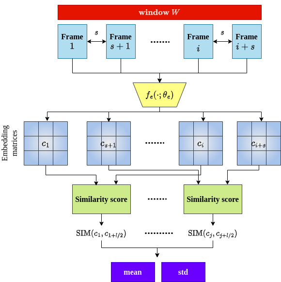
Figure 2: Similarity scoring calculation component of SeaDSC.

Once we have obtained the embedding matrices that represent our original images, we proceed to calculate the similarity score. Our hypothesis is that if the window undergoes a change in scenery, then the pair of frames at the start of the window will be different from the frame in the middle of the window. We calculate the similarity score between each pair of frames, specifically the $i$-th frame and the $(i+l/2)$-th frame within the window, rather than comparing consecutive frames. The specifics of how the similarity score is calculated are outlined in subsection 3.2.

Once the similarity score calculation is complete, we determine the mean and standard deviation values as a pair to represent the similarity score of the window. These values are used in the input for the change detection component.

3.1 Projection model

We utilize the VQ-VAE-2 algorithm [21] in our projection model $f_{e}(\cdot;\theta_{e})$. Compared to previous generative models, VQ-VAE-2 has superior lossy compression capabilities, allowing for training models on high-resolution photos. The fundamental concept behind VQ-VAE-2 involves training many hierarchical layers, where an input picture is compressed into quantized latent maps of varying sizes at each level. Vector quantization is a process that involves an encoder, which maps inputs to a series of discrete latent vectors, and a decoder, which reconstructs the inputs using these discrete vectors. To be more precise, when provided with an image $\mathrm{x}$, the encoder will apply a non-linear transformation to produce a vector $E(\mathrm{x})$. The vector is subsequently quantized by comparing its distance to a set of predefined vectors in the codebook list, resulting in the selection of a certain codebook $\mathrm{e}$. Similar to the previous work using VQ-VAE [27], the codebook for vector quantization is initialized using a uniform distribution as in the equation (1).

$$G\sim U(-\frac{1}{N_{e}},\frac{1}{N_{e}})$$ (1)

where $N_{e}$ is the size of codebook. The overall objective function is followed [21] and described in the equation (2).

$$\mathcal{L}(\mathrm{x},D(\mathrm{e}))=\mathcal{L}_{re}+\mathcal{L}_{vq}$$ (2)

where $\mathcal{L}_{re}$ and $\mathcal{L}_{vq}$ are the reconstruction loss and vector quantization loss which are defined in equations (3) and (4), respectively.

$$\mathcal{L}_{re}=\|\mathrm{x}-D(\mathrm{e})\|^{2}_{2}$$ (3)

$$\mathcal{L}_{vq}=\|sg[E(\mathrm{x})]-\mathrm{e}\|_{2}^{2}+\beta\|sg[\mathrm{e}]-E(\mathrm{x})\|^{2}_{2}$$ (4)

where $sg$ represents the stop gradient term. This term is initially set as the identity during forward computation and its partial derivatives are set to zero. Additionally, $\beta$ is a hyperparameter used for tuning. It affects the reluctance to modify the code associated with the encoder output.

3.2 Similarity score

Figure 3 depicts the procedure for calculating the similarity score between two embedding feature maps, $c_{u}$ and $c_{v}$. During this procedure, we initially partition each feature map into a grid consisting of cells of identical size, with $N_{cell}$ cells in total. Our primary idea for computing the similarity score between two feature maps involves partitioning the feature maps into a grid and then comparing the similarity of the associated cells in each grid. Intuitively, if two grids contain a greater number of pairs of comparable cells, their similarity score will be higher.

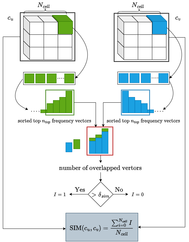
Figure 3: The diagram of similar estimation for two feature maps $c_{u}$ and $c_{v}$. $I$ is denoted for the indicator function, which two cells are similar ($I=1$) or not ($I=0$).

We iterate through a loop to calculate the similarity between two cells that have the same index in two grids. To begin with, we perform a process of flattening each cell feature, resulting in two sequences of discrete vectors. Next, we group the distinct discrete vector with its corresponding frequency and arrange them in descending order based on frequency. In the subsequent stage, we choose an equal number of top $n_{top}$ frequency distinct vectors from both sides and ascertain the count of overlapping distinct vectors between them. In the final stage, we assess the similarity between two cells by comparing the number of overlapping discrete vectors with a predetermined threshold, denoted as $\delta_{sim}$. Finally, we compute the similarity score between two feature maps, $c_{u}$ and $c_{v}$, by dividing the number of comparable cells by the total number of cells in the grid, $N_{cell}$.

4 Experiment

4.1 Experiment Setting

Datasets. We utilize a wide variety of data sets in our experiment. Firstly, we select a dataset to train our projection model. We create a training dataset by combining information from multiple sources. We have selected a cumulative sum of 10,000 images from three publicly available datasets: 3,000 images from the Singapore Maritime dataset [16], 3,000 images from the MODD2 dataset [1], and 4,000 images from the Seaships dataset [24]. To ensure an unbiased evaluation, we choose an alternative dataset to examine our system. We selected 35 videos from the RoboWhaler [3]. These videos are centered and have different durations. The total duration adds up to around 66.37 minutes, with each video being recorded at a frame rate of 12 frames per second. Therefore, a grand total of 47,681 frames were successfully retrieved. We categorize all of these videos by annotating each part into two unique categories: changed and not changed scenes. Out of the total number of frames, specifically 11,369 frames were found to be not scene changed, while the rest 36,312 frames were found to have scene changed.

Setting We do resizing of the image to the dimensions of $960\times 600\times 3$, while adding padding to match the width, height, and number of channels. The normalization of all photos is performed using a Gaussian distribution with a mean and standard deviation of 0.5. We set up two hierarchical layers for projection model. In the codebook of the VQ-VAE-2 projection model, we establish that the number of items, denoted as $N_{e}$, is 512. Every item in the code book consists of 64 discrete vectors. We use the feature map from bottom hierarchical with shape of the embedding feature is $150\times 240\times 64$. We implemented a dual-layer structure for the encoder network of the VQ-VAE-2 to enhance its efficiency and reduce its computational burden. The VQ-VAE-2 model contains a total of 1.3 million trainable parameters. The PyTorch library was used to create the model, which was trained for 100 epochs using the Adam optimizer [11] with a learning rate of $3e^{-}4$.

We use frame skipping with $s=4$ to optimize the evaluation process and reduce inference time. This means that we only consider every fourth frame, yielding a computation rate of three frames per second. To maximize computing efficiency, we do not use a stride window. We have established that the duration of each window is 10 seconds, which corresponds to $l=120$ frames. To calculate the similarity score, we setup $N_{cell}$ is 25 cells, $\delta_{sim}$ is 2, and $n_{top}$ is 5. We transform the feature map into a grid with dimensions of $5\times 5$. Each cell in the grid has dimensions of $30\times 48\times 64$. To calculate the similarity of grid-level, we specify that the number of most frequently occurring discrete vectors is 10, and the criterion for the top similarity of scalar vectors is 5. The change detection component utilizes the widely-used clustering algorithm K-Means [13] with a fixed number of clusters, specifically 2 clusters representing the categories of changed scene and unchanged scene. The execution of all steps is performed on the NVIDIA GeForce RTX 2080 Ti device, which has a capacity of 11 GB.

Evaluation metrics. We do applying the precision, recall and F1-score for evaluating scene change detection.

4.2 Results

Quantitative result. The Figure 4 and Table 1 display the comprehensive performance analysis of our SeaDSC technique. The results demonstrate that SeaDSC achieves a high level of accuracy in detecting dynamic scene changes, with a recall rate of 99%. However, the performance of detecting unchanged scenes is inferior. There are numerous transitional scenes that occur between a distinct, unaltered scene and a modified one that are unclear and challenging to identify. Adjusting the stride value during the sliding window process might enhance the accuracy in identifying scene boundaries. However, this adjustment may result in increased processing expenses during inference. This is the compromise between the expense of computing and the level of precision.

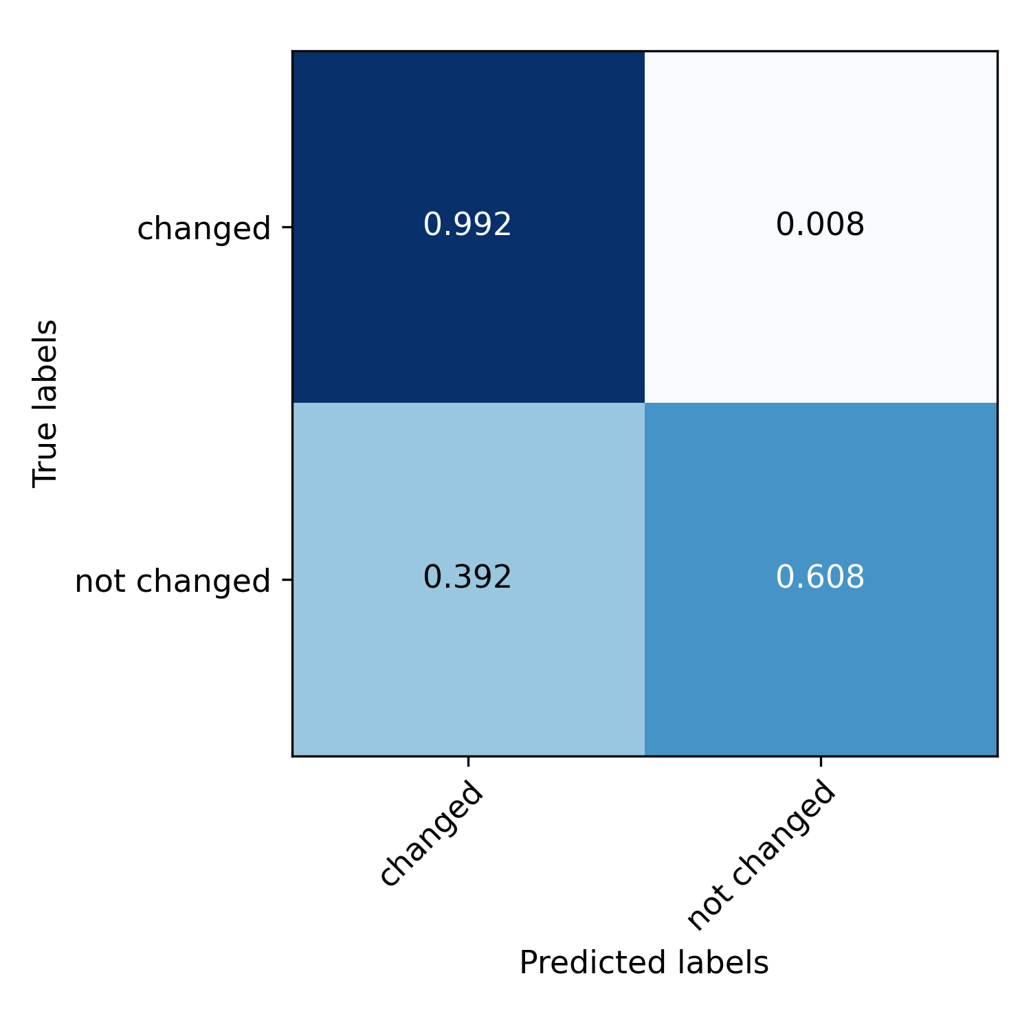
Figure 4: The confusion matrix results of SeaDSC.

The classification report in the Table 1 shows model’s performance in distinguishing between scene changed and not scene changed classes. The model’s precision, recall, and F1-score show differential performance between the two classes. For scene changed, the model has robust results with precision of 0.89, recall of 0.99, and F1-score of 0.94. However, it struggles with not scene changed, with a lower precision of 0.96 but a lower recall of 0.61. The overall accuracy of 0.9 across all samples supports the model’s ability to accurately predict both classes.

	Precision	Recall	F1-score	# Samples
changed	0.89	0.99	0.94	36,312
cot changed	0.96	0.61	0.74	11,369
Accuracy	0.9			47,681
Macro average	0.92	0.8	0.84	47,681
Weighted average	0.91	0.9	0.89	47,681

Table 1: The classification report results of SeaDSC.

Qualitative analysis. We randomly selected a few videos from the RoboWhaler dataset for qualitative analysis. The Figure 5 displays the qualitative analysis of two sampled videos. In this case, the photos were captured at regular intervals of 1.5 seconds from a specific portion of the film in order to clearly observe the transition between scenes. We additionally generate a graph illustrating the correlation between the predicted values (Pred) and the annotated values (GT). The Figure 5 show

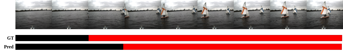
(a) Example on a part of video prodromos_2021_10_29_sailboats_busy.

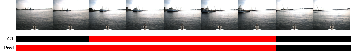
(b) Example on a part of video philos_2020_09_24_Gateway_Enveavor.

Figure 5: Example of qualitative results of SeaDSC on sampled data of RoboWhaler [3]. In these example, images in video here are sampled per 1.5 seconds. : not changed scene, : changed scene.

In Figure 5(a), the ground truth (GT) indicates that the scene did not change until the sailboat appeared closely in front of the USVs. However, the prediction incorrectly identifies a small section in the boundary of the modified scene as not being scene changed. The remaining predictions in the sequence accurately correspond to the ground truth. In a separate film, Figure 5(b) depicts a large ship in the distance moving at a slow pace towards the USV. The scenario remains unchanged throughout. However, our approach has inaccuracies in identifying the unchanged scene. In the subsequent portion of the video, the model accurately predicts alignment with the annotation. These instances of failure demonstrate that accurately identifying dynamic scene changes in tough scenarios remains a difficult task for implementing practical nautical vision applications.

5 Conclusion

This paper introduces our SeaDSC method, a framework for detecting dynamic scene changes in videos captured by USVs. Our framework consists of three primary components: a feature extraction that aims to project an image into an embedding feature, a similarity scoring component for calculating the magnitude of similarity inside video segments, and a clustering module that groups similar magnitudes into either scene changed or not scene changed segments. As a crucial element of our system, we provide a novel method for calculating similar magnitudes. Our method propose grid similarity calculation that relies on quantized discrete vectors. Our clustering process concludes with the utilization of the basic K-means algorithm. The experimental results on the maritime video dataset RoboWhaler with our annotated data demonstrate the efficacy of our approaches in terms of both accuracy and processing time, making them highly promising for real-world maritime applications. Furthermore, this work is the inaugural expansion into marine vision based on our current understanding. Our future work will involve expanding into another area of scene change detection, specifically semantic scene change detection for USVs.

6 Acknowledgments

The work was carried out in the framework of project INNO2MARE - Strengthening the Capacity for Excellence of Slovenian and Croatian Innovation Ecosystems to Support the Digital and Green Transitions of Maritime Regions (Funded by the European Union under the Horizon Europe Grant N°101087348).

References

- [1] Borja Bovcon, Rok Mandeljc, Janez Perš, and Matej Kristan. Stereo obstacle detection for unmanned surface vehicles by imu-assisted semantic segmentation. Robotics and Autonomous Systems, 104:1–13, 2018.
- [2] James E. Cutting, Jordan E. DeLong, and Kaitlin L. Brunick. Visual activity in hollywood film: 1935 to 2005 and beyond. Psychology of Aesthetics, Creativity, and the Arts, 5(2):115–125, 2011.
- [3] Michael DeFilippo, Michael Sacarny, and Paul Robinette. Robowhaler: A robotic vessel for marine autonomy and dataset collection. In OCEANS 2021: San Diego – Porto, pages 1–7, 2021.
- [4] Navid Dorfeshan and Mohammadreza Ramezanpour. Compressed domain scene change detection based on transform units distribution in high efficiency video coding standard. Journal of Computer & Robotics, 11(2):41–48, 2018.
- [5] Liang Du and Haibin Ling. Dynamic scene classification using redundant spatial scenelets. IEEE Transactions on Cybernetics, 46:2156–2165, 2016.
- [6] Badr Ben Elallid, Nabil Benamar, Abdelhakim Senhaji Hafid, Tajjeeddine Rachidi, and Nabil Mrani. A comprehensive survey on the application of deep and reinforcement learning approaches in autonomous driving. Journal of King Saud University - Computer and Information Sciences, 34(9):7366–7390, 2022.
- [7] Christoph Feichtenhofer, Axel Pinz, and Richard P. Wildes. Dynamic scene recognition with complementary spatiotemporal features. IEEE Transactions on Pattern Analysis and Machine Intelligence, 38(12):2389–2401, 2016.
- [8] Christoph Feichtenhofer, Axel Pinz, and Richard P. Wildes. Temporal residual networks for dynamic scene recognition. In 2017 IEEE Conference on Computer Vision and Pattern Recognition (CVPR), pages 7435–7444, 2017.
- [9] Aalok Gangopadhyay, Shivam Mani Tripathi, Ishan Jindal, and Shanmuganathan Raman. Sa-cnn: Dynamic scene classification using convolutional neural networks, 2015.
- [10] Sorin Grigorescu, Bogdan Trasnea, Tiberiu Cocias, and Gigel Macesanu. A survey of deep learning techniques for autonomous driving. Journal of Field Robotics, 37, 11 2019.
- [11] Diederik P. Kingma and Jimmy Ba. Adam: A method for stochastic optimization. In 3rd International Conference on Learning Representations, ICLR 2015, 2015.
- [12] Adarsh Kowdle and Tsuhan Chen. Learning to segment a video to clips based on scene and camera motion. In Computer Vision – ECCV 2012, pages 272–286, 2012.
- [13] S. Lloyd. Least squares quantization in pcm. IEEE Transactions on Information Theory, 28(2):129–137, 1982.
- [14] United Nations Conference on Trade and Development. Review of maritime transport 2023, 2023.
- [15] Xiaoming Peng, Abdesselam Bouzerdoum, and Son Phung. A trajectory-based method for dynamic scene recognition. International Journal of Pattern Recognition and Artificial Intelligence, 35:2150029, 05 2021.
- [16] Dilip K. Prasad, Deepu Rajan, Lily Rachmawati, Eshan Rajabally, and Chai Quek. Video processing from electro-optical sensors for object detection and tracking in a maritime environment: A survey. IEEE Transactions on Intelligent Transportation Systems, 18(8):1993–2016, 2017.
- [17] Dalei Qiao, Guangzhong Liu, Taizhi Lv, Wei Li, and Juan Zhang. Marine vision-based situational awareness using discriminative deep learning: A survey. Journal of Marine Science and Engineering, 9(4), 2021.
- [18] Yuanyuan Qiao, Jiaxin Yin, Wei Wang, Fábio Duarte, Jie Yang, and Carlo Ratti. Survey of deep learning for autonomous surface vehicles in marine environments. IEEE Transactions on Intelligent Transportation Systems, 24(4):3678–3701, 2023.
- [19] Giorgio Rascioni, Susanna Spinsante, and E. Gambi. An optimized dynamic scene change detection algorithm for h.264/avc encoded video sequences. International Journal of Digital Multimedia Broadcasting, 2010, 01 2010.
- [20] M. Rayatifard, M. Mehrabi, and M. Ghanbari. A fast and robust shot detection method in hevc/h.265 compressed video. Multimedia Tools and Applications, Oct 2023.
- [21] Ali Razavi, Aaron van den Oord, and Oriol Vinyals. Generating diverse high-fidelity images with vq-vae-2. In Advances in Neural Information Processing Systems, volume 32, 2019.
- [22] Iwin Thanakumar Joseph S., Sasikala J., and Sujitha Juliet D. Ship detection and recognition for offshore and inshore applications: a survey. International Journal of Intelligent Unmanned Systems, 7(4):177–188, Jan 2019.
- [23] Y. Salih and L. E. George. Dynamic scene change detection in video coding. International Journal of Engineering, 33(5):966–974, 2020.
- [24] Zhenfeng Shao, Wenjing Wu, Zhongyuan Wang, Wan Du, and Chengyuan Li. Seaships: A large-scale precisely annotated dataset for ship detection. IEEE Transactions on Multimedia, 20(10):2593–2604, 2018.
- [25] Dolley Shukla and Manisha Sharma. A novel video scene change detection using successive estimation of statistical measure and hibisli method. International Journal of Information Technology, 11(1):47–54, Mar 2019.
- [26] Li Su, Yusheng Chen, Hao Song, and Wanyi Li. A survey of maritime vision datasets. Multimedia Tools and Applications, 82(19):28873–28893, Aug 2023.
- [27] Linh Trinh, Bach Ha, and Anh Tu Tran. Vqc-covid-net: Vector quantization contrastive learning for covid-19 image base classification. In 2022 9th NAFOSTED Conference on Information and Computer Science (NICS), pages 247–251. IEEE, 2022.
- [28] Ruolan Zhang, Shaoxi Li, Guanfeng Ji, Xiuping Zhao, Jing Li, and Mingyang Pan. Survey on deep learning-based marine object detection. Journal of Advanced Transportation, 2021:1–18, 11 2021.