Optimal Hyperparameter $\epsilon$ for Adaptive Stochastic Optimizers through Gradient Histograms

Abstract

Optimizers are essential components for successfully training deep neural network models. In order to achieve the best performance from such models, designers need to carefully choose the optimizer hyperparameters. However, this can be a computationally expensive and time-consuming process. Although it is known that all optimizer hyperparameters must be tuned for maximum performance, there is still a lack of clarity regarding the individual influence of minor priority hyperparameters, including the safeguard factor $\epsilon$ and momentum factor $\beta$, in leading adaptive optimizers (specifically, those based on the Adam optimizers). In this manuscript, we introduce a new framework based on gradient histograms to analyze and justify important attributes of adaptive optimizers, such as their optimal performance and the relationships and dependencies among hyperparameters. Furthermore, we propose a novel gradient histogram-based algorithm that automatically estimates a reduced and accurate search space for the safeguard hyperparameter $\epsilon$, where the optimal value can be easily found.

1 Introduction

In the last decade, neural networks (NN) have gained much attention as an exceptional framework for many real-world applications, such as image classification [1], language processing [2], autonomous systems [3], and so on. As the NN models have become deeper and more complex, optimization algorithms, also known as optimizers, have progressively evolved to ensure proper training of these sophisticated models.

Gradient descent-based optimizers, categorized as either non-adaptive or adaptive, iteratively minimize an objective function by moving in the direction opposite to the gradient at a fixed or adaptive learning rate, i.e:

$$\theta_{t+1}=\theta_{t}-\alpha_{t}(\alpha,hyper)\odot{g}_{t}(hyper),$$ (1)

where $\alpha_{t}\in\mathbb{R}$ for the non-adaptive case, $\alpha_{t}\in\mathbb{R}^{N}$ for the adaptive case, $g_{t}$ is the gradient approximation, and $\alpha=\alpha_{0}$ is the initial learning rate hyperparameter. These methods requires a proper selection of hyperparameters to maximize performance (Fig. 1(a)) and avoid divergence (Fig. 1(b)) instead of relying on default hyperparameters. Although the learning rate $\alpha$ is considered one of the most important hyperparameters [4, 5] for both non-adaptive and adaptive optimizers, recent research [6] has shown that tuning all hyperparameters, including learning rate $\alpha$, safeguard factor $\epsilon$, first-order momentum $\beta_{1}$ and second-order momentum $\beta_{2}$, and learning rate schedule’s hyperparameters (decay steps and learning rate decay), can promote better performance, where adaptive optimizers can provide equivalent or superior effectiveness than non-adaptive ones. Nevertheless, hyperparameter search process demands a lot of computational effort for large-scale problems, even when using hyperparameter optimization techniques [4] such as Bayesian optimization and genetic algorithms.

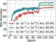
(a) VGG11 - CIFAR10

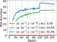
(b) VGG11 - Tiny ImageNet

Figure 1: Performance comparison of the Adam optimizer using default hyperparameters (red lines) versus tuned hyperparameters for training the VGG11 model on CIFAR-10 and Tiny ImageNet datasets.

To thoroughly examine the individual-level impact and significance of misclassified minor priority hyperparameters of adaptive optimizers, such as the safeguard factor $\epsilon$ and momentum factor $\beta$, and to efficiently determine their optimal values, in this work, from a new perspective based on gradient histograms, we present the following contributions:

• A novel framework based on gradient histograms is proposed to analyze adaptive optimizers and understand more precisely what happens when optimal hyperparameters are selected.

• Instead of depending on limited prior knowledge to establish a search space for finding the optimal safeguard hyperparameter $\epsilon$, a new algorithm based on gradient histograms is developed to automatically determine a reduced and accurate search range for this hyperparameter, where selecting the optimal value is a straightforward task.

• It is identified that very popular tasks (classification), typically used for evaluating new adaptive optimizers, are not suitable for this purpose. This is due to the fact that when the optimal safeguard hyperparameter $\epsilon$ is set, these adaptive optimizers manifest behavior resembling that of a single non-adaptive optimizer.

• Sharing strategies on how to save on computational expenses, such as assessing only the lower and upper extreme values of the estimated search space for selecting the optimal safeguard hyperparameter $\epsilon$.

The structure of the remaining manuscript is organized as follows: Section 2 provides a brief summary of stochastic optimizers and their hyperparameters. Section 3 delves into research regarding the safeguard hyperparameter $\epsilon$ and introduces a new framework based on gradient histograms in the context of adaptive optimizers and their associated safeguard hyperparameter. Experimental results are reported in Section 4. Finally, conclusions are stated in Section 5.

2 Stochastic Optimizers

2.1 Non-adaptive Optimizers

Let an empirical risk minimization problem with cost function of the form

$$F(\theta) =\frac{1}{M}\sum_{k=1}^{M}f(\theta,x_{k}),$$ (2)

$$\nabla F(\theta) =\frac{1}{M}\sum_{k=1}^{M}\nabla f(\theta,x_{t})$$ (3)

where $\theta$ is a set of parameters and $\{x_{1},\dots,x_{M}\}$ is the training data. Standard gradient descent is a basic optimization algorithm that computes the gradient Eq. 3 of the cost function over the entire dataset, however, it can require significant memory capacity for large datasets. Instead, stochastic gradient descent (SGD) [7] randomly selects a portion of dataset at each iteration to estimate the gradient with which parameter update is performed, i.e.

$$\nabla\widetilde{F}(\theta) =\frac{1}{|\mathcal{B}|}\sum_{k\in\mathcal{B}}\nabla f(\theta,x_{k})$$ (4)

where $\mathcal{B}\subset\{1,\dots,M\}$ is a subset of data (called mini-batch) with size of $|\mathcal{B}|$. The convergence of this last optimization algorithm can be improved by incorporating Polyak’s momentum (heavy ball method) [8], Nesterov’s accelerated gradient [9] or a combination of both methods. The choice of method depends on the nature of the optimization problem, deterministic or stochastic. The SGD+Momentum optimizer can be expressed as:

$$b_{t}=\mu\cdot b_{t-1}+(1-\gamma)\cdot g_{t}$$ (5)

$$\theta_{t+1}=\theta_{t}-\alpha_{t}\cdot b_{t}$$ (6)

where $g_{t}=\nabla\widetilde{F}(\theta_{t},x_{t})$ is the estimated gradient from a mini-batch at time step $t$, $\mu$ is momentum hyperparameter with typical value $\mu=0.9$, $\gamma$ is the dampening hyperparameter and $\alpha_{t}=\alpha$ is a single constant learning rate. If $\mu=\gamma$, then Eq. 5 reduces to the exponential moving average (EMA) of the gradients, generally contained in state-of-the-art adaptive algorithms.

2.2 Adaptive Optimizers

Adaptive optimization algorithms are utilized in deep learning to dynamically adjust the learning rate during the training process. In contrast to fixed learning rate based approaches such as vanilla SGD, SGD+Polyak’s Momentum and SGD+Nesterov’s accelerated method, adaptive optimizers consistently demonstrate faster convergence rate and good generalization performance across many tasks [10, 11, 12], for instance, image recognition, image segmentation and natural language processing.

Several attractive adaptive optimizers, including AdaGrad [13], RMSprop [14], Adam[15], can be synthesized by the following generic framework, presented in Algorithm 1, where $\phi(\cdot)$ and $\psi(\cdot)$ are commonly exponential moving averaging functions, $\mathcal{W}(\cdot)$ is an square root function, all operations are element-wise and $\alpha_{t}$ is the adaptive learning rate.

Algorithm 1 Generic framework of adaptive optimization methods

1:Learning rate hyperparameter $\alpha$, safeguard hyperparameter $\epsilon$, momentum hyperparameters $\beta_{1}$ and $\beta_{2}$, and sequence of functions $\{\phi_{t},\psi_{t}\}^{T}_{t=1}$

2:for $t=1$ to T do

3:     $m_{t}=\phi_{t}(g_{1},...,g_{t},\beta_{1}),$

4:     $v_{t}=\psi_{t}(g_{1},...,g_{t},\beta_{2}),~{}~{}~{}~{}\alpha_{t}=\dfrac{\alpha}{\mathcal{W}(v_{t},\epsilon)}$

5:     $\theta_{t+1}=\theta_{t}-\alpha_{t}\odot{m}_{t}$

6:end for

Particularly, the hyperparameters of these optimizers can be classified into two distinct categories: those related to gradient direction and those related to adaptive learning rates, that are linked to $m_{t}$ and $\alpha_{t}$, respectively. Among Adam-based optimizers, estimation of gradient direction is performed from an exponential moving average:

$$m_{t}=\beta_{1}\cdot m_{t-1}+(1-\beta_{1})\cdot g_{t}$$ (7)

where $\beta_{1}$ is the first-order momentum hyperparameter, and the averaging allows to reduce the noise variance of the gradients at each time step. The adaptive learning rates of such optimizers are primarily governed by three key hyperparameters: learning rate $\alpha$, second-order momentum $\beta_{2}$, and safeguard factor $\epsilon$. The first hyperparameter $\alpha$ is a positive scalar value that controls the length of step by which the model parameters are updated. In convex landscapes, a smaller or larger learning rate hyperparameter generates a slower or faster convergence, respectively. Nevertheless, choosing larger learning rates can also lead to situations where the optimization process overshoots and oscillates around the optimal solution. While manual tuning of the learning rate hyperparameter is necessary to enhance performance, as indicated in [5, 16], there exist techniques known as learning rate schedules that can periodically modify the learning rate over time. These schedules can apply linear, polynomial, or exponential adjustments at specific epochs, and may integrate other additional hyperparameters. Researchers have investigated various learning rate schedules in studies such as [1, 4, 17]. The second hyperparameter $\beta_{2}$, also referred to as the exponential decay rate for the second moment:

$$v_{t}=\beta_{2}\cdot v_{t-1}+(1-\beta_{2})\cdot g_{t}^{2},$$ (8)

determines the contribution of the exponential moving average of squared gradients. In essence, it defines the amount of previous squared gradient samples that are observed over a window of approximately 1/(1-$\beta_{2}$) time samples, where the regular value for $\beta_{2}$ is 0.999. Finally, hyperparameter $\epsilon$ is a small value conventionally used to prevent division by zero. In the case of RMSprop and Adam optimizers, the default values for the safeguard hyperparameter $\epsilon$ are $1e^{-6}$ and $1e^{-8}$, respectively. However, their optimal values in practice can differ depending on the characteristics of the problem and dataset.

3 All about hyperparameter $\epsilon$

3.1 Related Works

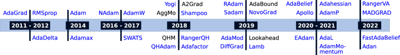
Figure 2: Timeline of adaptive optimizers, highlighted in blue those that contain the safeguard hyperparameter $\epsilon$ in their formulation.

In the deep learning field, a remarkable gap in terms of generalization performance exists between non-adaptive and adaptive stochastic optimizers, with the former demonstrating a distinct advantage, specifically in the context of computer vision applications. According to [5], the loss of generalization ability can be attributed to the unstable and extremely large adaptive learning rates that occur during training. To address this issue, new adaptive optimizers, e.g. AdaBound [18], RAdam [19], DiffGrad [20], AdaBelief [21], etc., have been developed to improve stability and accelerate convergence. Recently, [6] pointed out that standard adaptive optimizers, such as AdaGrad, RMsprop and Adam, which incorporate as a structural basis non-adaptive optimizers, never perform worse than the contained non-adaptive optimizers as long as all hyperparameters are carefully configured. Furthermore, this work reinforced the concept of tuning the safeguard hyperparameter $\epsilon$, as it, when combined with other hyperparameters, such as learning rate scheduling, enables the attainment of superior performance.

Literature evidence suggests that the default value of safeguard hyperparameter $\epsilon$ can be suboptimal for achieving peak performance. In fact, the optimal hyperparameter $\epsilon$ can be significantly larger, differing by orders of magnitude from the default setting. For example, the authors of [22] used $\epsilon=1.0$ for training their proposed Inception-V2 model on the ImageNet dataset with the RMSprop optimizer. In the same context but with $\epsilon=1e^{-3}$, [23] and [24] examined the performance of the MnasNet and EfficientNet models, respectively. Given the optimal safeguard value $\epsilon=1e^{-3}$, [25] compared the YOGI and Adam optimizers on the CIFAR-10 dataset for ResNet20, ResNet50 and DenseNet models. In neural machine translation, specifically for a transformer-based model trained on the WSLT’14 dataset, [19] showed that ADAM with $\epsilon=1e^{-4}$ outperformed ADAM with its default value $\epsilon=1e^{-8}$ in terms of convergence rate and minimum stable loss. For reinforcement learning task, [26] employed the Adam optimizer with a tuned safeguard value $\epsilon=1.5e^{-4}$.

The hyperparameter $\epsilon$ has been subject to some interpretations beyond its conventional role as a safeguard factor. For instance, [6] lists two alternative interpretations of this hyperparameter. First, by viewing ADAM as a diagonal approximation of natural gradient descent, $\epsilon$ can function as a damping factor that enhances the condition of Fisher [27]. Second, the hyperparameter $\epsilon$ can be seen as a trust region radius that regulates the effect of adaptability term $v_{t}$. In line with this second interpretation, [28] indicates that large $\epsilon$ can result in less adaptability, however, this latter interpretation has not been explored, and instead, a new optimizer that is independent of $\epsilon$ has been proposed as the main focus of the aforementioned research.

3.2 A New Perspective based on Gradient Histograms

In this section, we introduce an innovative framework, based on the gradient histograms, that enables to conduct a thorough analysis of adaptive optimizers and the safeguard hyperparameter $\epsilon$. Over the past few years, there has been a substantial increase in the development of various adaptive optimizers that depend on the hyperparameter $\epsilon$, as depicted in Fig. 2. Therefore, gaining an in-depth understanding of how this hyperparameter works is undoubtedly highly relevant to the field of machine learning.

Before delving into our proposed approach, it is essential to establish, as evidenced in Fig. 3, that in the case of an adaptive optimizer (such as the ADAM optimizer, as indicated in Eq. 9a, where $\hat{v}_{t}=v_{t}/(1-\beta_{2}^{t})$), a very small $\epsilon$ facilitates the adaptability of $\hat{v}_{t}$ up to the point of having a fully adaptive learning rate Eq. 9b, where $\epsilon$ is omitted due to its negligible impact. In the opposite situation, where $\epsilon$ is significantly large, the adaptability of $\hat{v}_{t}$ is attenuated, and in an extreme case, the adaptive learning rate is approximately a constant value, as outlined in Eq. 9c.

Taking into account that a large hyperparameter $\epsilon$ mitigates the adaptability offered by $\hat{v}_{t}$, we now label $\epsilon$ as immutability hyperparameter which can be opposed to adaptability, e.g. smaller immutability means higher adaptability of $\hat{v}_{t}$ and higher immutability means less adaptability of $\hat{v}_{t}$.

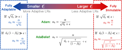
Figure 3: Influence of the safeguard hyperparameter $\epsilon$, renamed as immutability hyperparameter since it inversely affects adaptability of optimizers. For a comprehensive summary of the two extreme cases (fully adaptable and immutable) for some other adaptive optimizers, please review Table V of the Appendix A.

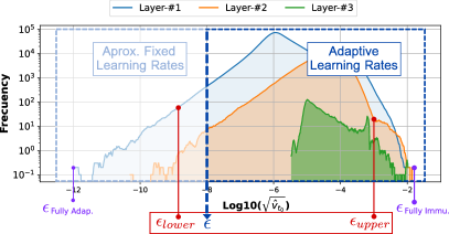
Figure 4: Gradient histograms for each layer^,hist-backpro at time $t_{0}$. Model presented is 1-Layer LSTM, where the LSTM layer is the Layer-$\#2$. Assuming an immutability value $\epsilon=1e^{-8}$ (vertical dashed blue line), gradients on the right-side end up generating adaptive learning rates, while gradients on the left-side, whose value are lower and much lower than $\epsilon$, results in approximately constant learning rates.

With the above information in consideration, it seems natural to ask how large or small the immutability hyperparameter $\epsilon$ must be to lie in any of the two extreme cases or to achieve the best optimizer performance. In order to have a reliable measure of this hyperparameter we propose to inspect the gradient histograms, that in particular for the Adam algorithm such histograms are computed from the adaptive term $\sqrt{\hat{v}_{t}}$. Using the gradient histograms, we can analyze the number of individual gradients that contribute to the adaptability of the optimizer during the training process. For example, in Fig. 2, we show, at time $t_{0}$, the gradient histograms of a 1-Layer LSTM model [29] trained with the Adam optimizer and a chosen immutability hyperparameter $\epsilon$. As can be seen, a large number of gradients are greater than the selected value of $\epsilon$ (vertical dashed blue line), which produce a large amount of dominant adaptive learning rates, i.e. the optimizer exhibit a high adaptability level at time $t_{0}$. However, in our experimental results, by monitoring the histograms, we also distinguish low and almost zero adaptability levels for Adam-based optimizers.

Furthermore, as detailed in next Section 3.3, from the proposed gradient histogram-based algorithm, we can automatically estimate an accurate and narrowed search range for the immutability hyperparameter $\epsilon$ of the adaptive optimizers, simplifying the process of finding the optimal value.

3.3 Optimal Search Space for the Immutability Hyperparameter $\epsilon$ using Gradient Histograms

Although manual search with a predefined range based on previous knowledge or random search with a broad range are common methodologies [4, 30], they have inherent limitations related to computational cost and inaccuracy when applied to new cases. Particularly, the optimal range for the immutability hyperparameter $\epsilon$ can differ by many orders of magnitude depending on the type of tasks, optimizers, models and datasets. Instead of empirically establishing a range for the immutability hyperparameter $\epsilon$ or requiring previous research experience to narrow it down, as reported in [6, 21, 31], we can automatically estimate a reduced search space based on the gradient histograms during the first epoch. To avoid outliers such as zero gradient values, our proposed algorithm, described in Algorithm 2, computes the upper and lower bounds across all layers from the lowest 2nd-percentile and the highest 98th-percentil of the gradient histograms to ensure that the natures of adaptive optimizers are approximately fully immutable and fully adaptable. For the Adam optimizer, the gradient histograms are calculated from $\hat{z_{t}}=\sqrt{\hat{v_{t}}}$, where $\hat{z_{t}}$ can be interpreted as a proxy to estimate the immutability hyperparameter. For other adaptive optimizers, you can find the $\hat{z_{t}}$ values summarized in Table V of Appendix A.

Algorithm 2 Computing search space for the immutable hyperparameter $\epsilon$.

1:$\phi_{1}(\cdot)$ and $\phi_{2}(\cdot)$ are functions that respectively return the 2nd and 98th percentiles of a histogram of gradients.

2:$\epsilon_{lower}$ and $\epsilon_{upper}$

3:for $t=1$ to T= № of iterations in 1 epoch do

4:     $g_{t,k}=\nabla f_{t,k}$

5:     $Compute~{}v_{t,k}~{}accordingly~{}Table~{}\ref{tab:FullCases}$

6:     for $k=1$ to K=№ of updated variables do

7:         if $t==T$ then

8:              $Compute~{}\hat{z}_{t,k}~{}accordingly~{}Table~{}\ref{tab:FullCases}$

9:              $Compute~{}Histogram~{}of~{}\hat{z}_{t,k}$

10:              $\epsilon_{lower}=min\{\epsilon_{lower},~{}\phi_{1}(Hist_{\hat{z}_{t,k}})\}$

11:              $\epsilon_{upper}=max\{\epsilon_{upper},~{}\phi_{2}(Hist_{\hat{z}_{t,k}})\}$

12:         end if

13:     end for

14:end for

15:$\epsilon_{lower}=10^{round(log10(\epsilon_{lower}))}$

16:$\epsilon_{upper}=10^{round(log10(\epsilon_{upper}))}$

In addition, there are some supplementary algorithmic details to consider, including: (i) As the computation of bounds is an iterative procedure, the initial values of $\epsilon_{lower}$ and $\epsilon_{upper}$ are set to the maximum value for the float32 data type and zero, respectively. (ii) For simplicity and less computational cost, our implementation uses a sort function to find the percentiles (boundaries) instead of directly calculating a histogram function.

4 Experimental Results

4.1 Simulation Scenario

We conduct two set of experiments to analyze the performance of adaptive optimizers from their specific gradient histograms, which are related with the immutability hyperparameter $\epsilon$. Particularly, this new framework based on the gradient histograms helps to better understand adaptive algorithms (Section 4.2) and to automatically estimate a precise and narrowed search space for the mentioned hyperparameter (Section 4.3). The experiments are structured as follows:

• NNs on image classification: VGG11 [32], DenseNet121 [33], ResNet34 [1], AlexNet [34] and MLP [35] models were trained on the CIFAR-10 [36], Tiny ImageNet [37] and Fashion-MNIST [38] datasets. It is important to note that not all datasets were used for training all models. For more details, please refer to Table I. We trained the models for 150 epochs with a batch size of 128 (except for the Tiny ImageNet dataset with a batch size of 32), a weight decay of $5e^{-4}$, and applied a learning rate decay of 0.1 at the 100-th epoch. For CIFAR-10 and Tiny ImageNet, we performed data augmentation that consists of random horizontal flipping, random cropping and z-score normalization, see coderefnotecode for numerical details.

• LSTM on language modeling: 1-Layer and 2-Layer LSTM models were trained from the Penn TreeBank [39] dataset. As [21], settings were 200 epochs with a batch size of 128, a weight decay of $1.2e^{-6}$, and applied a learning rate decay of 0.1 at the 100-th and 145-th epochs.

TABLE I: Details of the models for experiments.

Task	Dataset	Network Type	Architecture
Image Classification	CIFAR-10	Convolutional	VGG11, DenseNet121, ResNet34, AlexNet
	Tiny ImageNet	Convolutional	VGG11, AlexNet
	Fashion-MNIST	Non-convolutional	Multi Layer Perceptron
		Convolutional	AlexNet
Language Modeling	Penn TreeBank	Recurrent	1-Layer LSTM, 2-Layer LSTM

For clarity of the experimental analysis, we only examine the Adam optimizer with respect to the non-adaptive optimizer SGD+Momentum. In Fig. 5, we show the maximum performance achieved with the SGD+Momentum algorithm, which will be crucial for the final remarks in Section 4.2. Evaluation of other adaptive adaptive algorithms, including RSMprop, AdaBelief and AdaMomentum, may be found in Appendix A. Hyperparameters ($\alpha$, $\epsilon$, $\beta_{2}$) associated with adaptive learning rates $\alpha_{t}$ are carefully inspected and tuned, while the first-order momentum hyperparameter $\beta_{1}$, whose impact is not studied in this work, is set to its default value $\beta_{1}=0.9$. In order establish a reliable reference for the optimal search range of the Adam optimizer, we performed a grid search over a extensive range, varying the hyperparameters $\alpha$, $\epsilon$ and $(1-\beta_{2})$ in different powers of 10.

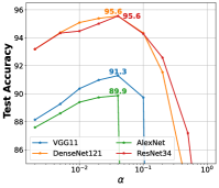
(a) Classification

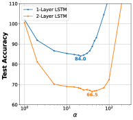
(b) Language modeling

Figure 5: Performance of deep learning models trained on the CIFAR-10 (left) and Penn TreeBank (right) datasets with SGD+Momentum, varying learning rate hyperapareter $\alpha$. For classification (a) higher accuracy equals better performance, whereas for language modeling (b) lower perplexity equals better performance.

4.2 Analysis of Adaptive Optimizers using Gradient Histograms

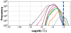
(a) VGG11 — Epoch 1 (beginning)

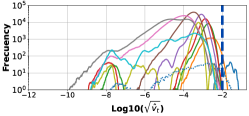
(b) VGG11 — Epoch 75 (middle)

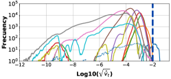
(c) VGG11 — Epoch 150 (end)

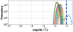
(d) DensNet121 — Epoch 1 (beginning)

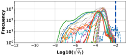
(e) DensNet121 — Epoch 75 (middle)

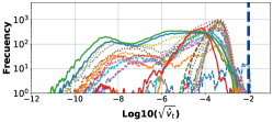
(f) DensNet121 — Epoch 150 (end)

Figure 8: Progress of gradient histograms of the VGG11 (top) and DenseNet121 (bottom) classifiers trained on the CIFAR-10 dataset with Adam and an immutability hyperparameter $\epsilon=1e^{-2}$. Vertical dashed blue line (chosen immutable hyperparameter $\epsilon$) marks the boundary of discarded elements, where gradients on the left-side are attenuated by $\epsilon$, resulting in approximately constant learning rates $\alpha_{t}\approx\alpha/\epsilon$, and gradients on the right-side generate adaptive learning rates.

As a baseline, for the classification and language modeling tasks, we present the performance of Adam optimizer when varying the learning rate $\alpha$ and immutability $\epsilon$, illustrated in Fig. 6 and Fig. 7 in the form of heatmaps.

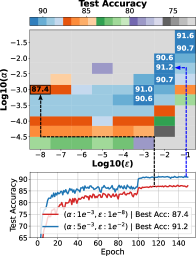
(a) VGG11

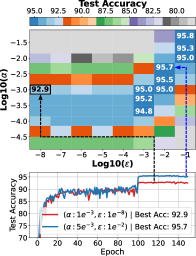
(b) DenseNet121

Figure 6: Classification task: Test accuracy of VGG11 and DenseNet121 models trained on the CIFAR-10 dataset with Adam, varying learning rate $\alpha$ and immutability $\epsilon$. For a given pair of hyperparameter values, each heatmap contains the highest accuracy achieved across all epochs.

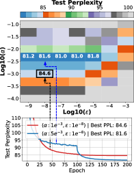
(a) 1-Layer LSTM

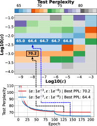
(b) 2-Layer LSTM

Figure 7: Language modeling task: Test perplexity of different LSTM models trained on the Penn TreeBank dataset with Adam, varying the learning rate $\alpha$ and immutability $\epsilon$. For a given pair of hyperparameter values, each heatmap contains the lowest perplexity achieved across all epochs. Better performance equals lower perplexity.

In both figures, we can observe that there is a subset of optimal learning rate $\alpha_{opt}$ and optimal immutability $\epsilon_{opt}$ that jointly maximize the optimizer performance, whose optimal immutability value can vary by orders of magnitude depending on the task. For example, in the Fig. 6 and Fig. 7, the optimal immutability values are $\epsilon_{opt}\geq 1e^{-3}$ and $\epsilon_{opt}\leq 1e^{-5}$ for classification task and language modeling task, respectively. Based on the information that can be extracted in these figures, it becomes challenging to address questions such as: Why do the optimal values of both hyperparameters ($\alpha$ and $\epsilon$) exhibit different linear relationships across different tasks? Why is a higher or lower value of immutability required to get the best results? Additionally, in Fig. 10, we show the performance obtained when varying second-order momentum hyperparameter $\beta_{2}$ w.r.t. the immutability, resulting in other types of patterns between them that will be explained later in this Section 4.2.

By analyzing the gradient histograms, presented in Fig. 8 and Fig. 9, we reveal novel and valuable information such as influence of the immutability hyperparameter $\epsilon$ and justification of the observed relationship between the $\alpha$ and $\epsilon$ hyperparameters, both insights will help to gain an improved comprehension of the behavior of adaptive optimizers. For the classification task, if an adaptive algorithm like Adam uses a large value of immutability hyperparameter, for example $\epsilon=1e^{-2}$ as in the Fig. 8, along with its corresponding optimal learning rate that guarantee the best performance, from the initial epoch only at most $0.33\%$ of elements in $\sqrt{\hat{v}_{t}}$ are greater than selected immutability hyperparameter (vertical dashed blue line), see Fig. 8 and Table II, meaning that $99.67\%$ of the elements in the denominator ($\sqrt{\hat{v}_{t}}+\epsilon$) of the adaptive optimization algorithm are approximately constant, since $\epsilon$ is the dominant term. In other words, given the large optimal value of immutability hyperparameter, the Adam algorithm at the beginning is basically similar to the SGD+Momentum algorithm (Eq. 5, where $\mu=\gamma=\beta_{1}$) with a near-constant adaptive learning rate $\alpha_{t}\approx\alpha/\epsilon$, and it consistently becomes more like SGD+Momentum after a some epochs, as the values of $\hat{v_{t}}$ get even smaller (evidenced by the evolution of the histograms in the Fig. 8). This pattern is also detected by training other well-known models such as AlexNet and ResNet34, or even using larger datasets such as Tiny ImageNet, where the classification task can be more complex, see also Fig. 13 to Fig. 15 in the Appendix A. From this new experimental evidence, the linear relation between $\alpha$ and $\epsilon$ observed for certain range of optimal values in the Fig. 6 is due to the fact that for said range, the Adam optimizer results to be similar to SGD+Momentum with approximately single learning rate $\alpha_{t}\approx\alpha/\epsilon$, where increasing $\alpha$ in the same proportion as $\epsilon$ gives the same $\alpha_{t}$.

TABLE II: Percentage of adaptive values $\sqrt{\hat{v_{t}}}$ greater than the chosen $\epsilon$ after the first epoch of training using Adam.

Dataset	Model	Immutability hyperparameter $\mathbf{\epsilon}$
		$\mathbf{1e^{-4}}$	$\mathbf{1e^{-3}}$	$\mathbf{1e^{-2}}$	$\mathbf{1e^{-1}}$
CIFAR-10	VGG11	61.50%	4.59%	0.33%	$2e^{-5}$%
	DenseNet121	98.40%	6.88%	0.10%	0%
Dataset	Model	Immutability hyperaparameter $\mathbf{\epsilon}$
		$\mathbf{1e^{-7}}$	$\mathbf{1e^{-6}}$	$\mathbf{1e^{-5}}$	$\mathbf{1e^{-4}}$
Penn TreeBank	1-Layer LSTM	100%	99.85%	91.88%	$9.14\%$
	2-Layer LSTM	$100\%$	$99.89\%$	$81.83\%$	$3.62\%$

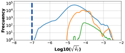
(a) 1-Layer LSTM — Epoch 1 (beginning)

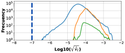
(b) 1-Layer LSTM — Epoch 100 (middle)

(c) 1-Layer LSTM — Epoch 200 (end)

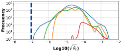
(d) 2-Layer LSTM — Epoch 1 (beginning)

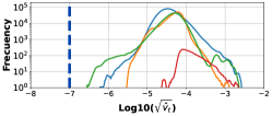
(e) 2-Layer LSTM — Epoch 100 (middle)

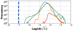
(f) 2-Layer LSTM — Epoch 200 (end)

Figure 9: Progress of gradient histograms of the 1-Layer LSTM and 2-Layer LSTM models trained on the Penn TreeBank dataset with Adam and an immutability hyperparameter $\epsilon=1e^{-7}$. Vertical dashed blue line (chosen immutable hyperparameter $\epsilon$) marks the boundary of discarded elements, where gradients on the left-side are attenuated by $\epsilon$, resulting in approximately constant learning rates $\alpha_{t}\approx\alpha/\epsilon$, and gradients on the right-side generate adaptive learning rates.

In this work, we additionally examine other adaptive optimizers, such as RMSprop [14], AdaBelief [21] and AdaMomentum [31], alongside the reported immutability hyperparameters $\epsilon$ from their respective publications, as presented in Fig. 16 and Fig.17 of Appendix A. It is important to highlight that the majority of adaptive optimizers proposed in the literature, including but not limited to RMSprop [14], DiffGrad [20], RAdan [19], AdaBelief [21], AdaMomentum [31], SWATS [40], have been extensively evaluated in the context of classification tasks, specifically on the CIFAR-10, CIFAR-100 and ImageNet datasets. In the Fig. 16, for the classification task, we can discern that the reported values of immutability hyperparameter $\epsilon$, which are optimal values, also suppresses the adaptability of the other evaluated optimizers from the first epoch onward, i.e. the other adaptive optimizers would be equivalent to the SGD+Momentum optimizer from the beginning for the aforementioned task. Due to this fact, in order to ensure a fair and meaningful basis for evaluating new adaptive optimizers in future research works, we recommend assessing these optimizers in alternative applications where the achieved performance depends on their intrinsic adaptability property. For this purpose, the following language modeling task can be an appropriate option to contemplate.

For language modeling task, plotted in the Fig. 7, the optimal values of immutability hyperparameter $\epsilon$ result to be small. By examining the gradient histograms in the Fig. 9, it is clear that all adaptive elements in $\sqrt{\hat{v}_{t}}$ are greater than the used optimal adaptability hyperparameter $\epsilon=1e^{-7}$ (vertical dashed blue line), producing 100% adaptive learning rates that contribute to the minimization, in contrast to the near-constant learning rates observed in the previous task. In essence, for this case, the superior performance of the Adam optimizer can be attributed to the full adaptability of its components. Furthermore, the largest optimal value of the immutability hyperparameter ($\epsilon\leq 1e^{-5}$) is associated with a high percentage of adaptive components (a high level of adaptability), the exact percentages are described in Table II. In this second case, concerning the relationship among hyperparameters, we can conclude that the optimal learning rate hyperparameter is independent of the immutability hyperparameter, as long as the immutability is less than adaptive term $\sqrt{\hat{v}_{t}}$.

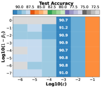
(a) VGG11 — $\{\alpha=1e^{-3}\}$

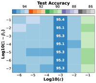
(b) DenseNet121 — $\{\alpha=5e^{-4}\}$

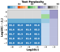
(c) 1-Layer LSTM — $\{\alpha=5e^{-3}\}$

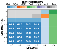
(d) 2-Layer LSTM — $\{\alpha=5e^{-3}\}$

Figure 10: Classification (top) and language modeling (bottom) tasks: Performance of VGG11 and DenseNet121 classifiers and 1-layer and 2-layer LSTM models trained on the CIFAR-10 and Penn TreeBank datasets, respectively, using the Adam optimizer. Performance is evaluated while varying the second-order momentum $\beta_{2}$ and the immutability $\epsilon$. Lower perplexity equals better performance.

Now, we will briefly examine the influence of the second-momentum hyperparameter $\beta_{2}$ on the two previous tasks. As expected, in the classification task with the optimal learning rate and immutability settings, and while varying the second-order momentum as depicted in Fig. 10(a) and 10(b), the Adam optimizer demonstrates independence from the second-order momentum value $\beta_{2}$. As mentioned earlier, this is because, in this case, the Adam optimizer structurally resembles an SGD+Momentum optimizer, where each element of adaptive learning rate ($\alpha_{t}\approx\alpha/\epsilon$) remains unaffected by $v_{t}$ and $\beta_{2}$. Clearly, tuning $\beta_{2}$ has no discernible impact on this task. For the language modeling task (as shown in Fig. 10(c) and 10(d)), where we know that $\sqrt{\hat{v}_{t}}>\epsilon$ and adaptability influences on the performance, we can see that within the optimal immutability range, there is an optimal range of second-order momentum hyperparameter. This latter range can be easily determined, considering at least that the optimal value of the second-order momentum must allow to average all batches of the dataset to obtain a $\sqrt{\hat{v_{t}}}$ that approximates the gradient distribution of all dataset. For instance, in the Fig. 10(c), training is done using approximately 668 batches of the Penn TreeBank dataset, given $N=1/(1-\beta_{2})$, where $N$ is the number of averaged samples, so $668\leq 1/(1-\beta_{2})\implies 0.9985\leq\beta_{2}$ to contemplate all dataset. Furthermore, as stated in [41], $\beta_{2}$ must be greater than $\beta_{1}$ and sufficiently distant to prevent convergence failure in general stochastic problems. Otherwise, Adam’s updates would be those of a sign stochastic gradient method.

Although these two cases show that adaptive optimizers like Adam can turn into either SGD+Momentum algorithm or fully adaptive algorithm, we do not rule out the possibility that there is a case where only partial adaptability associated with a moderate level of immutability, for example $50\%$ of dominant adaptive elements in $\sqrt{\hat{v}_{t}}$, can be essential to promote the best performance, while other higher or lower levels are not. Using the fashion-MNIST dataset, which is simpler compared to the CIFAR-10 and Tiny ImageNet datasets, for the classification task, we found, see Fig. 11 and Fig. 12, that the best optimizer performance is attained over a wide range of immutability hyperparameter values, implying a fully immutable (similar to SGD+Momentum), partially adaptable or fully adaptable behavior in the Adam algorithm without any practical difference between them.

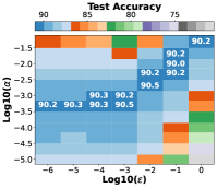
(a) Multi Layer Perceptron (MLP)

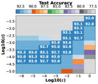
(b) AlexNet

Figure 11: Classification task: Test accuracy of different NN models trained on the Fashion-MNIST dataset with Adam, varying the learning rate $\alpha$ and immutability $\epsilon$.

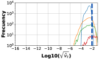
(a) $\epsilon=1e^{-2}$ $|$ Epoch 1 (beginning)

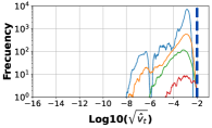
(b) $\epsilon=1e^{-2}$ $|$ Epoch 150 (end)

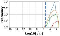
(c) $\epsilon=1e^{-5}$ $|$ Epoch 1 (beginning)

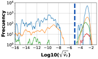
(d) $\epsilon=1e^{-5}$ $|$ Epoch 150 (end)

Figure 12: Comparison of gradient histograms of the MLP classifier trained on the FashionMNIST dataset with Adam, for two values of immutability hyperparameter.

Reflecting on these three tested cases, we wonder why the adaptive optimizers must be either fully immutable, fully adaptable, or of unimportant nature, the latter for the Fashion-MNIST case, to achieve the best performance? Before addressing this question, it is important to clarify that most of the adaptive learning rates can be interpreted as adaptive scale factors with normalization properties. In mathematical optimization field, an element-wise normalized gradient method [42], akin to RMSprop-based methods, is able to provide a fast progress on functions that contain flat regions, such as saddle points, and to be more useful than standard normalized gradient method when the flat regions are in some coordinates. From deep learning literature [12, 43, 44, 45], it is reasonable to assume that the effectiveness of an adaptive optimizer with specific characteristic, such as fully immutability (approximately SGD+Momentum) or fully adaptability, is intricately connected to convexity of the landscape.

Based on our previous experiments and the concept presented in [44], where critical point of a high-dimensional optimization problem can more certainly be a saddle point than a local minima, we infer that in the evaluated language modeling task, the landscape is probably non-convex with flat regions. Therefore, it is expected that an adaptive optimizer with the fully adaptive attribute (Fig. 7 and Fig. 9) outperforms an SGD+Momentum algorithm (Fig. 5(b)), which has slow crawling issues to pass through flat regions of saddle points. However, for the classification task, where the results showed that an adaptive optimizer closely resembling SGD+Momentum optimizer (Fig. 6) or the SGD+Momentum optimizer (Fig. 5(a)) yields the best performance, the landscape might be convex or approximately convex. In order to support this last assumption, we can take into account that [46] has theoretically proved that for a 2-layer network with ReLU activation, the landscape has no spurious local minima, which means a convex surface. In an approximately convex landscape, particularly near to the minima where the gradients are small, an adaptive optimizer can generate large learning rates, causing to be halt at higher point compare to the SGD+Momentum algorithm with smaller single learning rate, as observed in our first evaluated classification case (Fig. 6 and Fig. 8). Nevertheless, when the convex function has a sharper minima, the gradients in a neighbor close to the minimum are higher, so the adaptive learning rates can be small enough to match in performance as the SGD+Momentum algorithm without forcing large immutability factor. This statement must be happening in our last classification case (Fig.11 and Fig. 12).

4.3 Finding Optimal Search Space for the Immutability Hyperparameter $\epsilon$

In this final experimental section, we will validate the effectiveness of our straightforward algorithm in determining accurate search ranges of the immutability hyperparameters $\epsilon$ for the Adam optimizer and other adaptive optimizers.

Given the Adam optimizer, Table III shows the distinct search ranges used for the immutability hyperparameter $\epsilon$, where our predicted boundaries are highlighted in bold. As can be seen without prior information of how to pick limits, this is not our case, the reported search ranges in the literature might not contain the optimal immutability hyperparameter as observed in underlined ranges, resulting in an inferior performance for the Adam optimizer. For example, in the VGG11 model trained on CIFAR-10, if we use the suggested range ($\epsilon\in[1e^{-16},1e^{-5}]$) in [31], the maximum achieved accuracy is $89.1\%$, which falls $2.2\%$ short of our estimated range. This performance deficiency can be even greater (7.0 percentage points) when dealing with more complex classification tasks, as illustrated in Fig. 15(a) of Appendix A. Furthermore, it is worth noting that for the different trained models, our algorithm estimated a more accurate and compact range, which contains approximately 5 immutability combinations for testing instead of 12 to 21 combinations as reported in the literature [31, 6]. In Table IV, we also show the success of our algorithm in estimating the search range for other adaptive optimizers, consistently including the optimal immutability value that can differ depending on the task, model and optimizer employed.

Considering our estimated range and previous experimental findings, in order to get the best performance and to further reduce computational costs, we suggest evaluating only the two extreme values of the estimated immutability boundaries, or even trying the SGD+Momentum optimizer, which spends less training time, instead of using the Adam optimizer with the upper bound, as it is structurally and behaviorally similar to an SGD+Momentum optimizer. In both situations, given only one or two immutability values $\epsilon$, we are now concerned with varying the learning rate hyperparameter $\alpha$ to maximize performance. When choosing to train models with the SGD+Momentum optimizer (the second recommendation), note that its search space of the optimal learning rate hyperparameter $\alpha$ can vary drastically depending on the tasks (Fig. 5), while the optimal learning rate values of an adaptive optimizer are more centralized (Fig. 6 and Fig. 7), i.e. these have less variance across tasks.

TABLE III: Comparison of immutability hyperparameter ranges for the Adam optimizer in the classification and language modeling tasks. VGG, ResNet, AlexNet and DenseNet classifiers trained on CIFAR-10. LSTM models trained on Penn TreeBank, except for [6], 2-layer LSTM model trained on Tolstoy’s War and Peace.

Model	Optimal value	Tested Range on [31]	Tested Range on [6]	Our Estimated Range
VGG	$1e^{-3}\leq\epsilon_{opt}$	$[1e^{-16},1e^{-5}]$	$[1e^{-10},1e^{+10}]$	$\mathbf{[1e^{-6},1e^{-2}]}$
DenseNet	$1e^{-3}\leq\epsilon_{opt}$	$[1e^{-16},1e^{-5}]$	—	$\mathbf{[1e^{-4},1e^{-1}]}$
AlexNet	$1e^{-2}\leq\epsilon_{opt}$	—	—	$\mathbf{[1e^{-6},1e^{-2}]}$
ResNet	$1e^{-3}\leq\epsilon_{opt}$	$[1e^{-16},1e^{-5}]$	$[1e^{-10},1e^{+10}]$	$\mathbf{[1e^{-4},1e^{-1}]}$
1-Layer LSTM	$1e^{-5}\geq\epsilon_{opt}$	$[1e^{-16},1e^{-5}]$	—	$\mathbf{[1e^{-6},1e^{-2}]}$
2-Layer LSTM	$1e^{-5}\geq\epsilon_{opt}$	$[1e^{-16},1e^{-5}]$	$[1e^{-10},1e^{+10}]$	$\mathbf{[1e^{-7},1e^{-2}]}$

TABLE IV: Summary of the estimated immutability hyperparameter ranges for RMSProp, AdaBelief and AdaMomentum optimizers. VGG classifier trained on CIFAR-10. LSTM model trained on Penn TreeBank.

Task	Model	Optimizer	Optimal Value	Our Estimated Range
Classification	VGG	RMSProp	$1e^{-2}\leq\epsilon_{opt}$	$\mathbf{[1e^{-6},1e^{-2}]}$
		AdaBelief	$1e^{-8}\leq\epsilon_{opt}$	$\mathbf{[1e^{-17},1e^{-6}]}$
		AdaMo- mentum	$1e^{-10}\leq\epsilon_{opt}$	$\mathbf{[1e^{-16},1e^{-7}]}$
Language Modeling	1 Layer- LSTM	RMSProp	$1e^{-5}\geq\epsilon_{opt}$	$\mathbf{[1e^{-6},1e^{-2}]}$
		AdaBelief	$1e^{-14}\geq\epsilon_{opt}$	$\mathbf{[1e^{-15},1e^{-8}]}$
		AdaMo- mentum	$1e^{-14}\geq\epsilon_{opt}$	$\mathbf{[1e^{-16},1e^{-7}]}$

5 Conclusion

In conclusion, we putted forward two key contributions by considering a new perspective based on the gradient histograms that highly impacts in development of the deep learning field, specifically on the adaptive optimizers.

First, we presented mathematical and experimental evidence to support the behavior of adaptive optimizers, which can exhibit similar structural characteristics to the SGD+Momentum from the outset of training onward when the optimal safeguard hyperparameter $\epsilon$ (or immutability hyperparameter as previously defined) is set for the classification task. For investigations whose goal is to propose and assess new adaptive optimizers, we recommended avoiding this last task since the optimal value of immutability hyperparameter suppresses adaptive elements of $\alpha_{t}$, i.e. the adaptability property associated with learning rates is almost null. A better option for evaluating new adaptive optimizers is language modeling task. Furthermore, for a broader group of tasks, we identified and justified particular relationships and dependencies among hyperparameters such as learning rate $\alpha$, immutability $\epsilon$ and second-order momentum $\beta_{2}$.

Our second contribution focused on a novel algorithm that estimates an accurate and narrowed bounds for the optimal immutability hyperparameter $\epsilon$ of distinct state-of-the-art adaptive optimizers. Until now, this process has been based on trial and error to determine the optimal boundaries or optimal values, which could change drastically depending on deep learning tasks, optimizers, models and datasets. Likewise, direct use of the upper and lower bounds of the estimated range is recommended as primary strategy and potential optimal value to further reduce computational expenses.

Gustavo Silva received his B.Sc. degree in Electrical Engineering from the Ponticia Universidad Católica del Perú (PUCP), Lima, Peru, in 2015, and later earned his master’s degree in Digital Signal and Image Processing from the same university. Since 2015, he has been a collaborating researcher at the Digital Signal Processing Laboratory at said institution, where he has worked on projects related to signal and image processing, mathematical optimization and machine learning. He was an intern at Los Alamos National Laboratory (NM, USA), working on image processing and high-performance computing related projects. His research interests include image processing, optimization algorithms, computer vision, and deep learning.

Paul Rodriguez received the BSc degree in electrical engineering from the Pontificia Universidad Católica del Perú (PUCP), Lima, Peru, in 1997, and the MSc and PhD degrees in electrical engineering from the University of New Mexico, U.S., in 2003 and 2005 respectively. He spent two years (2005-2007) as a postdoctoral researcher at Los Alamos National Laboratory, and is currently a Full Professor with the Department of Electrical Engineering at PUCP. His research interests include AM-FM models, parallel algorithms, adaptive signal decompositions, and optimization algorithms (stochastic and non-stochastic) for inverse problems in signal and image processing such as Total Variation, Basis Pursuit, principal component pursuit (a.k.a. robust PCA), convolutional sparse representations, extreme learning machines, etc.

Appendix A Additional Experiments

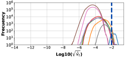
(a) AlexNet — Epoch 1 (beginning)

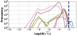
(b) AlexNet — Epoch 75 (middle)

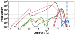
(c) AlexNet — Epoch 150 (end)

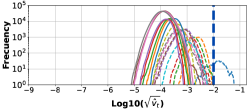
(d) ResNet34 — Epoch 1 (beginning)

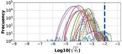
(e) ResNet34 — Epoch 75 (middle)

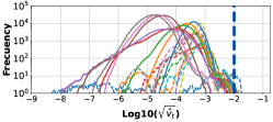
(f) ResNet34 — Epoch 150 (end)

Figure 14: Progress of gradient histograms of the AlexNet and ResNet34 classifiers trained on the CIFAR-10 dataset with Adam and an immutability hyperparameter $\epsilon=1e^{-2}$. Vertical dashed blue line (chosen immutable hyperparameter $\epsilon$) marks the boundary of discarded elements, where gradients on the left-side are attenuated by $\epsilon$, resulting in approximately constant learning rates $\alpha_{t}\approx\alpha/\epsilon$, and gradients on the right-side generate adaptive learning rates.

For a more thorough study of the classification task, in Fig. 13 to Fig. 15, we illustrate Adam optimizer performance when training AlexNet and ResNet models on the CIFAR-10 dataset, and when training VGG model using a more complex dataset (Tiny ImageNet dataset). Furthermore, for the classification and language modeling tasks, we also evaluate the behavior of other adaptive optimizers, including RMSprop [14], AdaBelief [21] and AdaMomentum [31], when an optimal value of immutability hyperparameter $\epsilon$ is selected, see Fig. 16 and Fig. 17.

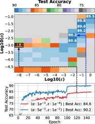
(a) AlexNet

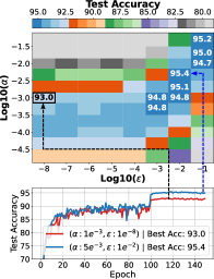
(b) ResNet34

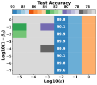
(c) AlexNet — $\{\alpha=5e^{-3}\}$

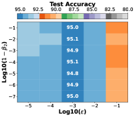
(d) ResNet34 — $\{\alpha=5e^{-4}\}$

Figure 13: Test accuracy of AlexNet and ResNet34 classifiers trained on the CIFAR-10 dataset with Adam optimizer, varying learning rate hyperparameter $\alpha$ vs immutability hyperparameter $\epsilon$ (top) and varying second-order momentum $\beta_{2}$ vs immutability hyperparameter $\epsilon$ (bottom).

For the classification task depicted in the Fig. 16, given the optimal immutability hyperparameter $\epsilon$, the RMSprop algorithm behaves similarly to the basic SGD algorithm throughout the entire training process. This is because the update direction in RMSprop is determined by the current gradient and its adaptive learning rate is approximately constant $\alpha_{t}\approx\alpha/\epsilon$. On the other hand, the AdaBelief and AdaMomentum optimizers tend to behave as the SGD+Momentum optimizer with $\alpha_{t}\approx\alpha/\epsilon$ and $\mu=\gamma=\beta_{1}$, denoted in Eq. 5 and Eq. 6.

For the language modeling task, as depicted in the Fig. 17, given the largest optimal values of immutability hyperparameter $\epsilon$ corresponding to the RMSprop, AdaBelief and AdaMomentum optimizers, $85.73\%$, $37.5\%$ and $39.51\%$ of adaptive elements are respectively greater than the chosen immutability values from start of training. Furthermore, if the optimal immutability hyperparameter $\epsilon$ is smaller value, which also guarantees best performance (refer to the leftmost column of the Fig. 17), there will be a greater number of dominant adaptive elements up to $100\%$, meaning a fully adaptive algorithm.

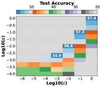
(a) VGG11

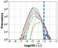
(b) VGG11 — Epoch 1 (beginning)

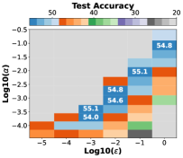
(c) AlexNet

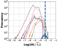
(d)

AlexNet — Epoch 1

(beginning)

Figure 15: Test accuracy of VGG11 and AlexNet classifiers trained on the Tiny ImageNet dataset using the Adam optimizer. Performance by varying learning rate hyperparameter $\alpha$ and immutability hyperparameter $\epsilon$ and gradient histograms at first epoch are assessed, where in the gradient histograms $0.17\%$ and $0.032\%$ of adaptive elements are greater than the chosen optimal values of immutability hyperparameter (vertical dashed blue line) for the respective classifiers.

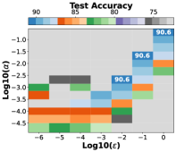
(a) RMSprop

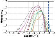
(b)

RMSprop — Epoch 1

(beginning)

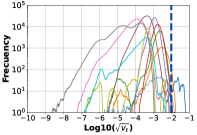
(c)

RMSprop — Epoch 75

(middle)

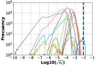
(d)

RMSprop — Epoch 150

(end)

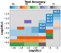
(e) AdaBelief

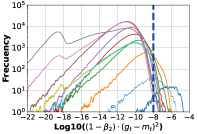
(f)

AdaBelief — Epoch 1

(beginning)

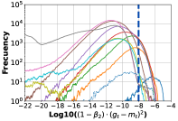
(g)

AdaBelief — Epoch 75

(middle)

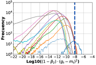
(h)

AdaBelief — Epoch 150

(end)

(i) AdaMomentum

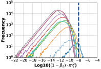
(j)

AdaMomentum — Epoch 1

(beginning)

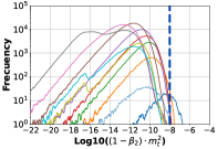
(k)

AdaMomentum — Epoch 75

(middle)

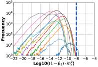
(l)

AdaMomentum — Epoch 150

(end)

Figure 16: Test accuracy of VGG11 classifier trained on the CIFAR-10 dataset with RMSprop, AdaBelief and AdaMomentum optimizers. In the first column, performance is evaluated by varying learning rate hyperparameter $\alpha$ and immutability hyperparameter $\epsilon$. In the second to fourth column. progress of gradient histograms is presented, where at first epoch $0.0051\%$, $0.68\%$ and $0.0062\%$ of adaptive elements are greater than the chosen optimal values of immutability hyperparameter (vertical dashed blue line) for the respective adaptive optimizers.

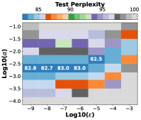
(a) RMSprop

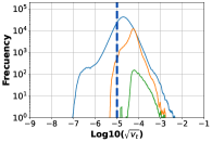
(b)

RMSprop — Epoch 1

(beginning)

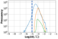
(c)

RMSprop — Epoch 100

(middle)

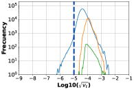
(d) RMSprop — Epoch 200 (end)

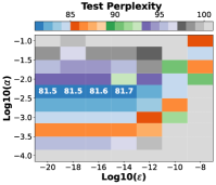
(e) AdaBelief

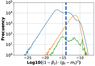
(f)

AdaBelief — Epoch 1

(beginning)

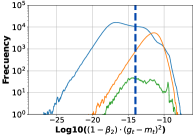
(g)

AdaBelief — Epoch 75

(middle)

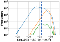
(h)

AdaBelief — Epoch 200

(end)

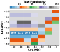
(i) AdaMomentum

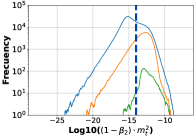
(j)

AdaMomentum — Epoch 1

(beginning)

(k)

AdaMomentum — Epoch 100

(middle)

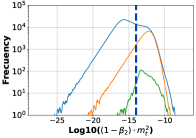
(l)

AdaMomentum — Epoch 200

(end)

Figure 17: Test perplexity of 1-Layer LSTM model trained on the Penn TreeBank dataset with RMSprop, AdaBelief and AdaMomentum. In the first column, performance is evaluated by varying learning rate hyperparameter $\alpha$ and immutability hyperparameter $\epsilon$, where lower perplexity corresponds to better performance. In the second to fourth column, progress of gradient histograms is presented, where at first epoch $85.73\%$, $37.5\%$ and $39.51\%$ of adaptive elements are greater than the chosen highest optimal values of immutability hyperparameter (vertical dashed blue line) for the respective adaptive optimizers.

TABLE V: Summary of adaptive learning rates. For the chosen value of hyperparameter $\epsilon$ is contemplated two extreme cases (fully adaptable and fully immutable), where each element of estimated adaptive learning rate $\alpha_{t}$ can be self-adjusting or approximately constant.

Optimizer	Adaptive Learning Rate	Fully Adaptable Case	Fully Immutable Case
AdaGrad	$\begin{array}[]{l}v_{t}=v_{t-1}+g_{t}^{2}\\ \alpha_{t}=\dfrac{\alpha}{\sqrt{v_{t}}+\epsilon}\\ \end{array}$	$\begin{array}[]{l}\hat{z}_{t}=\sqrt{v_{t}}\\ \text{If}~{}~{}\big{(}\hat{z}_{t}\gg\epsilon\big{)}:~{}~{}~{}\alpha_{t}\approx\dfrac{\alpha}{\sqrt{v_{t}}}\vspace{1.25mm}\end{array}$	$\begin{array}[]{l}\hat{z}_{t}=\sqrt{v_{t}}\\ \text{If}~{}~{}\big{(}\hat{z}_{t}\ll\epsilon\big{)}:~{}~{}~{}\alpha_{t}\approx\dfrac{\alpha}{\epsilon}\vspace{1.25mm}\end{array}$
RMSprop	$\begin{array}[]{l}v_{t}=\beta\cdot v_{t-1}+(1-\beta)\cdot g_{t}^{2}\\ \alpha_{t}=\dfrac{\alpha}{\sqrt{v_{t}}+\epsilon}\\ \end{array}$	$\begin{array}[]{l}\hat{z}_{t}=\sqrt{v_{t}}\\ \text{If}~{}~{}\big{(}\hat{z}_{t}\gg\epsilon\big{)}:~{}~{}~{}\alpha_{t}\approx\dfrac{\alpha}{\sqrt{v_{t}}}\vspace{1.25mm}\end{array}$	$\begin{array}[]{l}\hat{z}_{t}=\sqrt{v_{t}}\\ \text{If}~{}~{}\big{(}\hat{z}_{t}\ll\epsilon\big{)}:~{}~{}~{}\alpha_{t}\approx\dfrac{\alpha}{\epsilon}\vspace{1.25mm}\end{array}$
Adam	$\begin{array}[]{l}v_{t}=\beta_{2}\cdot v_{t-1}+(1-\beta_{2})\cdot g_{t}^{2}\\ \hat{{v}}_{t}=v_{t}/(1-\beta_{2}^{t})\\ \alpha_{t}=\dfrac{\alpha}{\sqrt{\hat{{v}_{t}}}+\epsilon}\vspace{1.25mm}\end{array}$	$\begin{array}[]{l}\hat{z}_{t}=\sqrt{\hat{v}_{t}}\\ \text{If}~{}~{}\big{(}\hat{z}_{t}\gg\epsilon\big{)}:\\ ~{}~{}~{}~{}~{}~{}~{}\alpha_{t}\approx\dfrac{\alpha}{\sqrt{\hat{{v}_{t}}}}\end{array}$	$\begin{array}[]{l}\hat{z}_{t}=\sqrt{\hat{v}_{t}}\\ \text{If}~{}~{}\big{(}\hat{z}_{t}\ll\epsilon\big{)}:\\ ~{}~{}~{}~{}~{}~{}~{}\alpha_{t}\approx\dfrac{\alpha}{\epsilon}\end{array}$
DiffGrad	$\begin{array}[]{l}\xi_{t}=1/(1+e^{-|g_{t-1}-g_{t}|}),\\ \text{where }0.5\leq\xi_{t}\leq 1\\ v_{t}=\beta_{2}\cdot v_{t-1}+(1-\beta_{2})\cdot g_{t}^{2}\\ \hat{{v}}_{t}=v_{t}/(1-\beta_{2}^{t})\\ \alpha_{t}=\dfrac{\alpha\cdot\xi_{t}}{\sqrt{\hat{{v}_{t}}}+\epsilon}\vspace{1.25mm}\end{array}$	$\begin{array}[]{l}\hat{z}_{t}=\sqrt{\hat{v}_{t}}\\ \text{If}~{}~{}\big{(}\hat{z}_{t}\gg\epsilon\big{)}:\vspace{1.25mm}\\ ~{}~{}~{}~{}~{}~{}~{}\alpha_{t}\approx\dfrac{\alpha\cdot\xi_{t}}{\sqrt{\hat{{v}_{t}}}}\vspace{2mm}\\ \\ \end{array}$	$\begin{array}[]{l}\hat{z}_{t}=\sqrt{\hat{v}_{t}}\\ \text{If}~{}~{}\big{(}\hat{z}_{t}\ll\epsilon\big{)}:\vspace{1.25mm}\\ ~{}~{}~{}~{}~{}~{}~{}\dfrac{\alpha}{2\cdot\epsilon}\leq\alpha_{t}\leq\dfrac{\alpha}{\epsilon},\vspace{2mm}\\ ~{}~{}~{}~{}~{}~{}~{}\text{where $\alpha_{t}\approx\dfrac{\alpha\cdot\xi_{t}}{\epsilon}$}\end{array}$
AdaMod	$\begin{array}[]{l}v_{t}=\beta_{2}\cdot v_{t-1}+(1-\beta_{2})\cdot g_{t}^{2}\\ \hat{{v}}_{t}=v_{t}/(1-\beta_{2}^{t})\\ n_{t}=\dfrac{\alpha}{\sqrt{\hat{{v}_{t}}}+\epsilon}\\ s_{t}=\beta_{3}\cdot s_{t-1}+(1-\beta_{3})\cdot n_{t}\\ \alpha_{t}=\min\{n_{t},s_{t}\}\vspace{1.25mm}\end{array}$	$\begin{array}[]{l}\hat{z}_{t}=\sqrt{\hat{v}_{t}}\\ \text{If}~{}~{}\big{(}\hat{z}_{t}\gg\epsilon\big{)}:\\ ~{}~{}~{}~{}~{}~{}~{}n_{t}\approx\dfrac{\alpha}{\sqrt{\hat{{v}_{t}}}}\\ ~{}~{}~{}~{}~{}~{}~{}s_{t}=\beta_{3}\cdot s_{t-1}+(1-\beta_{3})\cdot n_{t}\\ ~{}~{}~{}~{}~{}~{}~{}\alpha_{t}=\min\{n_{t},s_{t}\}\end{array}$	$\begin{array}[]{l}\hat{z}_{t}=\sqrt{\hat{v}_{t}}\\ \text{If}~{}~{}\big{(}\hat{z}_{t}\ll\epsilon\big{)}:\\ ~{}~{}~{}~{}~{}~{}~{}n_{t}\approx\dfrac{\alpha}{\epsilon}\\ ~{}~{}~{}~{}~{}~{}~{}\alpha_{t}=(1-\beta_{3}^{t})\cdot\dfrac{\alpha}{\epsilon}\\ \\ \end{array}$
$\begin{array}[]{c}\textbf{AdaBelief}\end{array}$	$\begin{array}[]{l}v_{t}=\beta_{2}\cdot v_{t-1}+(1-\beta_{2})\cdot(g_{t}-m_{t})^{2}\\ s_{t}=v_{t}+(1-\beta_{2}^{t})\cdot\epsilon/(1-\beta_{2})\\ \hat{{s}}_{t}=s_{t}/(1-\beta_{2}^{t})=\hat{{v}}_{t}+\epsilon/(1-\beta_{2})\\ \alpha_{t}=\dfrac{\alpha}{\sqrt{\hat{{s}_{t}}}+\epsilon}\vspace{1.25mm}\end{array}$	$\begin{array}[]{l}\hat{z}_{t}=(1-\beta_{2})\cdot\hat{v}_{t}\\ \text{If}~{}~{}\big{(}\hat{z}_{t}\gg\epsilon\big{)}:\\ ~{}~{}~{}~{}~{}~{}~{}s_{t}\approx\beta_{2}\cdot s_{t-1}+(1-\beta_{2})\cdot(g_{t}-m_{t})^{2}\\ ~{}~{}~{}~{}~{}~{}~{}\alpha_{t}\approx\dfrac{\alpha}{\sqrt{\hat{{s}_{t}}}}\vspace{1.25mm}\end{array}$	$\begin{array}[]{l}\hat{z}_{t}=(1-\beta_{2})\cdot\hat{v}_{t}\\ \text{If}~{}~{}\big{(}\hat{z}_{t}\ll\epsilon\big{)}:\\ ~{}~{}~{}~{}~{}~{}~{}s_{t}\approx\beta_{2}\cdot s_{t-1}+\epsilon\\ ~{}~{}~{}~{}~{}~{}~{}\alpha_{t}\approx\dfrac{\alpha}{\sqrt{\epsilon/(1-\beta_{2})}+\epsilon}\vspace{1.25mm}\end{array}$
MADGRAD	$\begin{array}[]{l}\lambda_{t}=\alpha\sqrt{t+1}\\ v_{t}=v_{t-1}+\lambda_{t}\cdot g_{t}^{2}\\ \alpha_{t}=\dfrac{1}{\sqrt[3]{v_{t}}+\epsilon}\vspace{1.25mm}\end{array}$	$\begin{array}[]{l}\hat{z}_{t}=\sqrt[3]{v_{t}}\\ \text{If}~{}~{}\big{(}\hat{z}_{t}\gg\epsilon\big{)}:\vspace{1.25mm}\\ ~{}~{}~{}~{}~{}~{}~{}\alpha_{t}\approx\dfrac{1}{\sqrt[3]{v_{t}}}\vspace{1.25mm}\end{array}$	$\begin{array}[]{l}\hat{z}_{t}=\sqrt[3]{v_{t}}\\ \text{If}~{}~{}\big{(}\hat{z}_{t}\ll\epsilon\big{)}:\vspace{1.25mm}\\ ~{}~{}~{}~{}~{}~{}~{}\alpha_{t}\approx\dfrac{1}{\epsilon}\end{array}$
$\begin{array}[]{c}\textbf{EAdam}\footref{refnote}\end{array}$	$\begin{array}[]{l}v_{t}=\beta_{2}\cdot v_{t-1}+(1-\beta_{2})\cdot g_{t}^{2}\\ s_{t}=v_{t}+(1-\beta_{2}^{t})\cdot\epsilon/(1-\beta_{2})\\ \hat{{s}}_{t}=s_{t}/(1-\beta_{2}^{t})=\hat{{v}}_{t}+\epsilon/(1-\beta_{2})\\ \alpha_{t}=\dfrac{\alpha}{\sqrt{\hat{{s}_{t}}}}\vspace{1.25mm}\end{array}$	$\begin{array}[]{l}\hat{z}_{t}=(1-\beta_{2})\cdot\hat{v}_{t}\\ \text{If}~{}~{}\big{(}\hat{z}_{t}\gg\epsilon\big{)}:\\ ~{}~{}~{}~{}~{}~{}~{}s_{t}\approx\beta_{2}\cdot s_{t-1}+(1-\beta_{2})\cdot g_{t}^{2}\\ ~{}~{}~{}~{}~{}~{}~{}\alpha_{t}\approx\dfrac{\alpha}{\sqrt{\hat{{s}_{t}}}}\vspace{1.25mm}\end{array}$	$\begin{array}[]{l}\hat{z}_{t}=(1-\beta_{2})\cdot\hat{v}_{t}\\ \text{If}~{}~{}\big{(}\hat{z}_{t}\ll\epsilon\big{)}:\\ ~{}~{}~{}~{}~{}~{}~{}s_{t}\approx\beta_{2}\cdot s_{t-1}+\epsilon\\ ~{}~{}~{}~{}~{}~{}~{}\alpha_{t}\approx\dfrac{\alpha}{\sqrt{\epsilon/(1-\beta_{2})}}\vspace{1.25mm}\end{array}$
$\begin{array}[]{c}\textbf{AdaMo-}\vspace{-1.5mm}\\ \textbf{mentum}\footref{refnote}\end{array}$	$\begin{array}[]{l}v_{t}=\beta_{2}\cdot v_{t-1}+(1-\beta_{2})\cdot m_{t}^{2}\\ s_{t}=v_{t}+(1-\beta_{2}^{t})\cdot\epsilon/(1-\beta_{2})\\ \hat{{s}}_{t}=s_{t}/(1-\beta_{2}^{t})=\hat{{v}}_{t}+\epsilon/(1-\beta_{2})\\ \alpha_{t}=\dfrac{\alpha}{\sqrt{\hat{{s}_{t}}}}\vspace{1.25mm}\end{array}$	$\begin{array}[]{l}\hat{z}_{t}=(1-\beta_{2})\cdot\hat{v}_{t}\\ \text{If}~{}~{}\big{(}\hat{z}_{t}\gg\epsilon\big{)}:\\ ~{}~{}~{}~{}~{}~{}~{}s_{t}\approx\beta_{2}\cdot s_{t-1}+(1-\beta_{2})\cdot m_{t}^{2}\\ ~{}~{}~{}~{}~{}~{}~{}\alpha_{t}\approx\dfrac{\alpha}{\sqrt{\hat{{s}_{t}}}}\vspace{1.25mm}\end{array}$	$\begin{array}[]{l}\hat{z}_{t}=(1-\beta_{2})\cdot\hat{v}_{t}\\ \text{If}~{}~{}\big{(}\hat{z}_{t}\ll\epsilon\big{)}:\\ ~{}~{}~{}~{}~{}~{}~{}s_{t}\approx\beta_{2}\cdot s_{t-1}+\epsilon\\ ~{}~{}~{}~{}~{}~{}~{}\alpha_{t}\approx\dfrac{\alpha}{\sqrt{\epsilon/(1-\beta_{2})}}\vspace{1.25mm}\end{array}$

References

- [1] K. He, X. Zhang, S. Ren, and J. Sun, “Deep residual learning for image recognition,” in Proceedings of the IEEE conference on computer vision and pattern recognition, 2016, pp. 770–778.
- [2] C. D. Manning, M. Surdeanu, J. Bauer, J. R. Finkel, S. Bethard, and D. McClosky, “The stanford corenlp natural language processing toolkit,” in Proceedings of 52nd annual meeting of the association for computational linguistics: system demonstrations, 2014, pp. 55–60.
- [3] V. Mnih, K. Kavukcuoglu, D. Silver, A. A. Rusu, J. Veness, M. G. Bellemare, A. Graves, M. Riedmiller, A. K. Fidjeland, G. Ostrovski et al., “Human-level control through deep reinforcement learning,” nature, vol. 518, no. 7540, pp. 529–533, 2015.
- [4] T. Yu and H. Zhu, “Hyper-parameter optimization: A review of algorithms and applications,” arXiv preprint arXiv:2003.05689, 2020.
- [5] A. C. Wilson, R. Roelofs, M. Stern, N. Srebro, and B. Recht, “The marginal value of adaptive gradient methods in machine learning,” Advances in neural information processing systems, vol. 30, 2017.
- [6] D. Choi, C. J. Shallue, Z. Nado, J. Lee, C. J. Maddison, and G. E. Dahl, “On empirical comparisons of optimizers for deep learning,” arXiv preprint arXiv:1910.05446, 2019.
- [7] H. Robbins and S. Monro, “A stochastic approximation method,” The annals of mathematical statistics, pp. 400–407, 1951.
- [8] N. Qian, “On the momentum term in gradient descent learning algorithms,” Neural networks, vol. 12, no. 1, pp. 145–151, 1999.
- [9] Y. E. Nesterov, “A method of solving a convex programming problem with convergence rate o(k^2),” in Doklady Akademii Nauk, vol. 269, no. 3. Russian Academy of Sciences, 1983, pp. 543–547.
- [10] J. R. Sashank, K. Satyen, and K. Sanjiv, “On the convergence of adam and beyond,” in International conference on learning representations, vol. 5, 2018, p. 7.
- [11] W. Shen, X. Wang, Y. Wang, X. Bai, and Z. Zhang, “Deepcontour: A deep convolutional feature learned by positive-sharing loss for contour detection,” in Proceedings of the IEEE conference on computer vision and pattern recognition, 2015, pp. 3982–3991.
- [12] N. S. Keskar, D. Mudigere, J. Nocedal, M. Smelyanskiy, and P. T. P. Tang, “On large-batch training for deep learning: Generalization gap and sharp minima,” arXiv preprint arXiv:1609.04836, 2016.
- [13] J. Duchi, E. Hazan, and Y. Singer, “Adaptive subgradient methods for online learning and stochastic optimization.” Journal of machine learning research, vol. 12, no. 7, 2011.
- [14] T. Tieleman and G. Hinton, “Lecture 6.5-rmsprop, coursera: Neural networks for machine learning,” University of Toronto, Technical Report, vol. 6, 2012.
- [15] D. P. Kingma and J. Ba, “Adam: A method for stochastic optimization,” arXiv preprint arXiv:1412.6980, 2014.
- [16] L. N. Smith and N. Topin, “Super-convergence: Very fast training of neural networks using large learning rates,” in Artificial intelligence and machine learning for multi-domain operations applications, vol. 11006. SPIE, 2019, pp. 369–386.
- [17] L. N. Smith, “Cyclical learning rates for training neural networks,” in 2017 IEEE winter conference on applications of computer vision (WACV). IEEE, 2017, pp. 464–472.
- [18] L. Luo, Y. Xiong, Y. Liu, and X. Sun, “Adaptive gradient methods with dynamic bound of learning rate,” arXiv preprint arXiv:1902.09843, 2019.
- [19] L. Liu, H. Jiang, P. He, W. Chen, X. Liu, J. Gao, and J. Han, “On the variance of the adaptive learning rate and beyond,” arXiv preprint arXiv:1908.03265, 2019.
- [20] S. R. Dubey, S. Chakraborty, S. K. Roy, S. Mukherjee, S. K. Singh, and B. B. Chaudhuri, “diffgrad: an optimization method for convolutional neural networks,” IEEE transactions on neural networks and learning systems, vol. 31, no. 11, pp. 4500–4511, 2019.
- [21] J. Zhuang, T. Tang, Y. Ding, S. C. Tatikonda, N. Dvornek, X. Papademetris, and J. Duncan, “Adabelief optimizer: Adapting stepsizes by the belief in observed gradients,” Advances in neural information processing systems, vol. 33, pp. 18 795–18 806, 2020.
- [22] C. Szegedy, V. Vanhoucke, S. Ioffe, J. Shlens, and Z. Wojna, “Rethinking the inception architecture for computer vision,” in Proceedings of the IEEE conference on computer vision and pattern recognition, 2016, pp. 2818–2826.
- [23] M. Tan, B. Chen, R. Pang, V. Vasudevan, M. Sandler, A. Howard, and Q. V. Le, “Mnasnet: Platform-aware neural architecture search for mobile,” in Proceedings of the IEEE/CVF conference on computer vision and pattern recognition, 2019, pp. 2820–2828.
- [24] M. Tan and Q. Le, “Efficientnet: Rethinking model scaling for convolutional neural networks,” in International conference on machine learning. PMLR, 2019, pp. 6105–6114.
- [25] M. Zaheer, S. Reddi, D. Sachan, S. Kale, and S. Kumar, “Adaptive methods for nonconvex optimization,” Advances in neural information processing systems, vol. 31, 2018.
- [26] M. Hessel, J. Modayil, H. Van Hasselt, T. Schaul, G. Ostrovski, W. Dabney, D. Horgan, B. Piot, M. Azar, and D. Silver, “Rainbow: Combining improvements in deep reinforcement learning,” in Proceedings of the AAAI conference on artificial intelligence, vol. 32, no. 1, 2018.
- [27] J. Martens and R. Grosse, “Optimizing neural networks with kronecker-factored approximate curvature,” in International conference on machine learning. PMLR, 2015, pp. 2408–2417.
- [28] P. Savarese, D. McAllester, S. Babu, and M. Maire, “Domain-independent dominance of adaptive methods,” in Proceedings of the IEEE/CVF Conference on Computer Vision and Pattern Recognition, 2021, pp. 16 286–16 295.
- [29] X. Ma, Z. Tao, Y. Wang, H. Yu, and Y. Wang, “Long short-term memory neural network for traffic speed prediction using remote microwave sensor data,” Transportation Research Part C: Emerging Technologies, vol. 54, pp. 187–197, 2015.
- [30] J. Bergstra and Y. Bengio, “Random search for hyper-parameter optimization.” Journal of machine learning research, vol. 13, no. 2, 2012.
- [31] Y. Wang, Y. Kang, C. Qin, H. Wang, Y. Xu, Y. Zhang, and Y. Fu, “Rethinking adam: A twofold exponential moving average approach,” arXiv preprint arXiv:2106.11514, 2021.
- [32] K. Simonyan and A. Zisserman, “Very deep convolutional networks for large-scale image recognition,” arXiv preprint arXiv:1409.1556, 2014.
- [33] G. Huang, Z. Liu, L. Van Der Maaten, and K. Q. Weinberger, “Densely connected convolutional networks,” in Proceedings of the IEEE conference on computer vision and pattern recognition, 2017, pp. 4700–4708.
- [34] A. Krizhevsky, I. Sutskever, and G. E. Hinton, “Imagenet classification with deep convolutional neural networks,” Communications of the ACM, vol. 60, no. 6, pp. 84–90, 2017.
- [35] C. M. Bishop et al., Neural networks for pattern recognition. Oxford university press, 1995.
- [36] A. Krizhevsky, G. Hinton et al., “Learning multiple layers of features from tiny images,” 2009.
- [37] Y. Le and X. Yang, “Tiny imagenet visual recognition challenge,” CS 231N, vol. 7, no. 7, p. 3, 2015.
- [38] H. Xiao, K. Rasul, and R. Vollgraf, “Fashion-mnist: a novel image dataset for benchmarking machine learning algorithms,” arXiv preprint arXiv:1708.07747, 2017.
- [39] M. Marcus, B. Santorini, and M. A. Marcinkiewicz, “Building a large annotated corpus of english: The penn treebank,” 1993.
- [40] N. S. Keskar and R. Socher, “Improving generalization performance by switching from adam to sgd,” arXiv preprint arXiv:1712.07628, 2017.
- [41] S. J. Reddi, S. Kale, and S. Kumar, “On the convergence of adam and beyond,” arXiv preprint arXiv:1904.09237, 2019.
- [42] J. Watt, R. Borhani, and A. K. Katsaggelos, Machine learning refined: Foundations, algorithms, and applications. Cambridge University Press, 2020.
- [43] A. Choromanska, M. Henaff, M. Mathieu, G. B. Arous, and Y. LeCun, “The loss surfaces of multilayer networks,” in Artificial intelligence and statistics. PMLR, 2015, pp. 192–204.
- [44] Y. N. Dauphin, R. Pascanu, C. Gulcehre, K. Cho, S. Ganguli, and Y. Bengio, “Identifying and attacking the saddle point problem in high-dimensional non-convex optimization,” Advances in neural information processing systems, vol. 27, 2014.
- [45] C. Zhang, S. Bengio, M. Hardt, B. Recht, and O. Vinyals, “Understanding deep learning (still) requires rethinking generalization,” Communications of the ACM, vol. 64, no. 3, pp. 107–115, 2021.
- [46] Y. Wang, J. Lacotte, and M. Pilanci, “The hidden convex optimization landscape of regularized two-layer relu networks: an exact characterization of optimal solutions,” in International Conference on Learning Representations, 2021.