Selective Single and Double-Mode Quantum Limited Amplifier

Abstract

A quantum-limited amplifier enables the amplification of weak signals while introducing minimal noise dictated by the principles of quantum mechanics. These amplifiers serve a broad spectrum of applications in quantum computing, including fast and accurate readout of superconducting qubits and spins, as well as various uses in quantum sensing and metrology. Parametric amplification, primarily developed using Josephson junctions, has evolved into the leading technology for highly effective microwave measurements within quantum circuits. Despite their significant contributions, these amplifiers face fundamental limitations, such as their inability to handle high powers, sensitivity to parasitic magnetic fields, and particularly their limitation to operate only at millikelvin temperatures. To tackle these challenges, here we experimentally develop a novel quantum-limited amplifier based on superconducting kinetic inductance and present an extensive theoretical model to describe this nonlinear coupled-mode system. Our device surpasses the conventional constraints associated with Josephson junction amplifiers by operating at much higher temperatures up to 4.5 K. With two distinct spectral modes and tunability through bias current, this amplifier can operate selectively in both single and double-mode amplification regimes near the quantum noise limit. Utilizing a nonlinear thin film exhibiting kinetic inductance, our device attains gain exceeding 50 dB in a single-mode and 32 dB in a double-mode configuration while adding $0.35$ input-referred quanta of noise. Importantly, this amplifier eliminates the need for Josephson junctions, resulting in significantly higher power handling capabilities than Josephson-based amplifiers. It also demonstrates resilience in the presence of magnetic fields, offers a straightforward design, and enhances reliability. This positions the amplifier as a versatile solution for quantum applications and facilitates its integration into future superconducting quantum computers.

I Introduction

Parametric amplifiers with noise characteristics at the quantum limit play a central role in quantum processors [1, 2], offering significant applications across various quantum systems [3, 4]. In the microwave frequency range [5, 6, 7, 8, 9, 10] these amplifiers enable precise, fast, and high-fidelity single-shot measurements of superconducting qubits [11, 12, 13, 14], ensembles of spins [15], quantum dots [16, 17], and nanomechanical resonators [18]. Furthermore, the utilization of near-quantum-limited amplifiers has created new experimental avenues for producing nonclassical radiation, including single and double-mode vacuum squeezing [19, 20, 21] with applications in weak measurement [22, 23], Axion dark matter detection [24, 25, 26, 27] and quantum illumination and radar [28, 29, 30, 31].

The most common method for building microwave parametric amplifiers involves superconducting Josephson junctions, configured as a Josephson Parametric Amplifier (JPA) [32, 33] or Josephson Traveling Wave Parametric Amplifier (JTWPA) [8, 9, 10]. These systems exploit the nonlinear characteristics of Josephson junctions to attain significant amplification with minimal noise. Through precise control facilitated by an external microwave pump, JPAs allow for fine-tuning of gain, enabling accurate and efficient amplification of weak signals. Their tunability and instantaneous bandwidth make quantum-limited amplifiers essential tools for advancing quantum information processing and pushing the boundaries of quantum technologies.

Despite their many valuable applications, both JPAs and JTWPAs encounter significant limitations that restrict their effective integration into scalable quantum architectures. Both JPAs and JTWPAs have a limited saturation input power, primarily attributed to the presence of higher-order nonlinearity such as the Kerr nonlinearity. This limitation typically confines them to operate only with a few microwave photons per bandwidth [5, 34] and thus limits their ability to effectively handle a wide range of frequencies and higher-power signals. Moreover, Josephson-based amplifiers are highly sensitive to parasitic magnetic fields, which can negatively impact their performance. To mitigate this sensitivity, magnetic field isolation is often necessary. Furthermore, they typically require operation at temperatures below 1 Kelvin [5, 9, 10], which can pose practical challenges in applications where higher temperature operation is desired [28, 29, 30].

An alternative approach to overcome these limitations involves the building of quantum-limited amplifiers without the reliance on Josephson junctions by using superconducting films that possess kinetic inductance. This approach utilizes a simplified single-step lithography process and employs thin films of high-temperature kinetic inductance superconductors, such as Niobium Titanium Nitride (NbTiN) [35, 36, 37, 38, 39, 40]. The intrinsic kinetic inductance of the NbTiN film introduces the necessary nonlinearity for achieving quantum-limited amplification, thereby eliminating the need to use Josephson junctions. These amplifiers typically use Three-Wave Mixing (3WM) [38, 39, 40] or Four-Wave Mixing (4WM) [41, 42] processes to amplify the input signal. The amplification can happen through degenerate or non-degenerate parametric amplification [1, 2]. In the case of degenerate or phase-preserving amplification, the idler and signal have identical frequencies. This configuration offers the potential for noiseless amplification and the generation of single-mode vacuum squeezing [20, 43]. In contrast, in non-degenerate or phase-insensitive amplification, the idler and signal exist as separate modes with distinct frequencies. Within this regime, the amplifier’s output can be a two-mode squeezed state or an entangled state [2, 44]. Resonance-based kinetic inductance amplifiers primarily operate in the single mode configuration, functioning within degenerate or near non-degenerate amplification regimes [40]. In these configurations, shifting the pump frequency from twice the resonance frequency effectively initiates a 3WM process, wherein a pump photon is downconverted to idler and signal photons within the resonator mode. However, this approach encounters limitations, particularly when there is a requirement for generating two-mode squeezing and entanglement. This is primarily because the idler and signal do not represent two spectrally separated modes. Consequently, the development of a quantum-limited amplifier that is tunable, low-noise, compatible with high temperatures, and possesses the ability to selectively operate in both single and two-mode regimes, remains an outstanding challenge.

In this work, we introduce a quantum-limited Kinetic Inductance Resonance Parametric Amplifier (KIRPA) that overcomes some of the technical limitations associated with Josephson junction amplifiers and is capable of operating at higher temperatures due to the high critical temperature of the kinetic inductance thin film [45]. The presence of two spectrally and spatially distinct modes, along with the ability to tune the resonance frequency by applying bias current, enables the KIPRA to operate selectively in both single and dual-mode amplification regimes. By utilizing a uniformly evaporated thin film of NbTiN on high-resistivity intrinsic silicon, we achieve exceptional amplification, surpassing 50 dB gain in single mode and 32 dB gain in double mode configurations, respectively, with a gain-bandwidth product of approximately 30 MHz when operating in the 3WM regime. Importantly, our design eliminates the reliance on Josephson junctions, resulting in a significantly higher 1 dB compression point for the output power when compared to amplifiers based on Josephson technology [46]. The junction-free design of the KIRPA also allows a high degree of resilience to stray magnetic fields or adaptability to experiments requiring strong magnetic fields, reaching up to $2$ T [47, 48, 41, 42]. Additionally, compared to other kinetic inductance amplifiers [40], the design of our KIRPA is inherently simple and does not require complex circuitry or filtering to generate amplification. Utilizing kinetic inductance for amplification simplifies the design and fabrication processes to a remarkable degree compared to Josephson-based amplifiers. Moreover, it enhances reliability since the non-linearity of our device is an inherent feature of its geometry, eliminating the need for complicated and delicate fabrication procedures. Additionally, we introduce a theoretical model that describes the dynamics of the system and utilize it to fit the experimental results.

The paper is organized as follows: In Section II, we establish a comprehensive theoretical model to elucidate single-mode and double-mode amplification based on a coupled mode system. Section III introduces the experimental setup and the KIRPA design. Section IV presents the experimental results of single-mode and double-mode amplification. In Section V, we discuss the noise properties of the KIRPA and study the operation of the device in different device temperatures. Finally, the concluding remarks and discussions will be presented in Section VI.

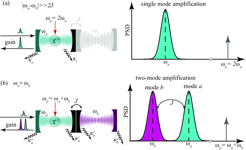
Figure 1: A schematic representation of a coupled resonator system exhibiting a coupling rate $J$. Here, one resonator, with resonance frequency $\omega_{a}$ and annihilation operator $a$, is coupled to an auxiliary resonator having resonance frequency $\omega_{b}$ and annihilation operator $b$. Incorporating a nonlinear medium characterized by a $\chi^{(2)}$ nonlinearity, resonator $a$ facilitates amplification via the Three-Wave-Mixing (3WM) process. The system’s operation mode, whether single-mode or double-mode amplification, can be selected by properly pumping the system. (a) Illustrates the single-mode amplification scenario, characterized by a significant separation in resonance frequencies between the two resonators, expressed as $|\omega_{a}-\omega_{b}|\gg 2J$. In this setup, the system can be effectively treated as a single mode by disregarding the dynamics of the auxiliary resonator $b$. Amplification of the single mode is achieved by applying a strong pump at $\omega_{p}=2\omega_{a}$, resulting in a degenerate amplification in mode $a$, as seen in the power spectral density (PSD) of the output field. (b) In contrast, by adjusting the resonance frequencies of the two modes to be equal, i.e., $\omega_{a}=\omega_{b}$ and pumping the system at $\omega_{p}=\omega_{a}+\omega_{b}$, double-mode amplification is realized, with the two modes being spectrally separated by the coupling rate $J$. Here, $\kappa_{j}^{e(i)}$ is the extrinsic (intrinsic) damping rate of each resonator $j=a,b$.

II Theoretical modeling of amplification

In this section, we provide an in-depth theoretical model that describes the 3WM process and amplification within a generic two-mode coupled system. In the subsequent sections, we divide our discussions into single-mode and two-mode amplification, and we construct separate comprehensive theoretical models for each of these regimes.

II.1 Hamiltonian

The system under consideration includes a coupled system that incorporates nonlinearity in one of the modes, as shown in Fig. 1. The Hamiltonian describing this coupled-mode system, accounting for parametric processes and operating in the presence of a pump with a frequency $\omega_{p}$ and an annihilation operator $a_{p}$, can be written as (with $\hbar=1$)

$$H=\omega_{a}a^{\dagger}a+\omega_{b}b^{\dagger}b+\omega_{p}a_{p}^{\dagger}a_{p}+J(a^{\dagger}b+b^{\dagger}a)+H_{\text{non}}.$$ (1)

where $a$ and $b$ are the annihilation operators of each mode with frequencies $\omega_{a}$ and $\omega_{b}$, respectively, and with coherent mode coupling strength $J$. We also define the nonlinear Hamiltonian [49, 40]

$$H_{\text{non}}=\frac{g_{0}}{2}(a^{2}a_{p}^{\dagger}+a^{\dagger 2}a_{p})+Ka^{\dagger 2}a^{2},$$ (2)

where the second term in this Hamiltonian describes the degenerate parametric interaction with strength $g_{0}$ and the third term represents a four-wave mixing interaction with strength $K$. In this Hamiltonian, the inclusion of nonlinearity in one of the modes results in an interesting scenario where we can operate the device in either single or double-mode amplification regimes. This choice can be made by tuning the resonance frequency of mode $a$, either far from or close to the anticrossing point, where efficient exchange of energy between the two modes occurs. We also note that, for our KIRPA in the presence of a strong bias current, $K\ll g_{0}$, and therefore the four-wave mixing process can be neglected. With a film thickness of 10 nm and a resonator of width $2\,\mu$m, the estimated Kerr nonlinearity will be approximately $K\approx 1$ mHz. As we will see later, this value is a few orders of magnitude smaller for the auxiliary resonator $b$.

II.2 Single mode amplification

Away from the anticrossing point, where the frequency of mode $a$ is well-separated from the auxiliary mode $b$, the interaction between these modes does not facilitate photon hopping or exchange of the excitation. Consequently, mode $b$ does not undergo amplification when $|\omega_{a}-\omega_{b}|\gg 2J$. In this case, we can treat the system as a single mode, characterized by substantial nonlinearity in mode $a$, see Fig. 1a. Therefore the Hamiltonian of the system in the strong pump regime is given by (see Supplementary Materials)

$$H=\Delta a^{\dagger}a+\frac{g}{2}(a^{2}e^{-i\phi_{p}}+a^{\dagger 2}e^{i\phi_{p}}),$$ (3)

where $g=g_{0}|\alpha_{p}|$ and $|\alpha_{p}|$ is the amplitude of the pump and $\phi_{p}$ is the global phase set by the pump. The above Hamiltonian has been written in a reference frame rotating at $\omega_{p}/2=\omega_{a}-\Delta$.

The system’s output can be written with respect to the input quantum noise ($a_{\mathrm{e}}$ with an extrinsic damping rate of $\kappa_{\mathrm{e}}$) and the intrinsic losses in the resonator mode (expressed as $a_{\mathrm{i}}$ with an intrinsic damping rate of $\kappa_{\mathrm{i}}$). Solving the quantum Langevin equations allows us to obtain the output field of the resonator (see Supplementary Materials)

$$a_{\mathrm{out}}(\omega) = \Big{[}\mathcal{G}_{S}(\omega)a_{\text{e}}+\mathcal{G}_{I}(\omega)a_{\text{e}}^{\dagger}\Big{]}$$ (4)

$$+ \sqrt{\frac{1-\eta}{\eta}}\Big{[}(\mathcal{G}_{S}(\omega)+1)a_{\text{i}}+\mathcal{G}_{I}(\omega)a_{\text{i}}^{\dagger}\Big{]}$$

where $\eta=\frac{\kappa_{\text{e}}}{\kappa}$ describes the waveguide-resonator coupling with $\kappa=\kappa_{\text{e}}+\kappa_{\text{i}}$ and we define

$$\mathcal{G}_{S}(\omega) = \frac{\eta\kappa\Big{[}\frac{\kappa}{2}-i(\omega+\Delta)\Big{]}}{\Delta^{2}-g^{2}+(i\omega-\frac{\kappa}{2})^{2}}+1,$$

$$\mathcal{G}_{I}(\omega) = \frac{i\eta\kappa ge^{i\phi}}{\Delta^{2}-g^{2}+(i\omega-\frac{\kappa}{2})^{2}},$$ (5)

Note that $|\mathcal{G}_{I}(\omega)|^{2}=|\mathcal{G}_{S}(\omega)|^{2}-1$ for $\eta\approx 1$. The first two terms of Eq. (4) show the amplification of the signal $a_{S}\equiv a_{e}$ and idler $a_{I}\equiv a_{e}^{\dagger}$ modes while the last two terms represent the noise terms added by the KIRPA due to the intrinsic loss of the resonator. In the absence of the internal loss $\eta\rightarrow 1$, Eq. (4) simplifies to $a_{\mathrm{out}}(\omega)=\sqrt{G}a_{\text{e}}+\sqrt{G-1}a_{\text{e}}^{\dagger}$, describing the annihilation operator of a degenerate (phase-sensitive) parametric amplifier with gain

$$G=|\mathcal{G}_{S}|^{2}=\Big{(}\frac{2}{1-4(g/\kappa)^{2}}-1\Big{)}^{2}$$ (6)

here for simplicity, we consider $\Delta=\omega=0$. We can see that for $g\ll\kappa$ the gain is negligible $G\rightarrow 1$. However, the highest level of gain is achieved near the denominator’s roots and as $g\rightarrow\kappa/2$ which results in $G\rightarrow\infty$. This divergence can be understood better by looking at the stability condition of the system through the susceptibility of the resonator [50]. For $\Delta=0$, the resonator’s susceptibility is given by (see the Supplementary Materials)

$$\bm{\chi}(\omega)=\frac{1}{(i\omega-\frac{\kappa}{2})^{2}-g^{2}}\begin{bmatrix}-i\omega+\frac{\kappa}{2}&-ige^{i\phi_{p}}\\ ige^{-i\phi_{p}}&-i\omega+\frac{\kappa}{2}\end{bmatrix}$$ (7)

The stability of the system is determined by the denominator of $\bm{\chi}(0)$, imposing $g<\kappa/2$ as the stability criteria [2]. This condition ensures that the parametric amplifier operates below its threshold and avoids entering self-sustained oscillations. However, when $g\geq\kappa/2$ the system becomes unstable and it leads to parametric self-oscillations.

II.3 Double-mode amplification

The result in Eq. (4) can be extended to non-degenerate, phase-insensitive amplification, where we deal with two spectrally distinct signal and idler modes. This can be achieved by bringing mode $a$ on resonance with mode $b$, see Fig 1b. The coherent interaction between the two modes, when combined with the 3WM process in mode $a$, enables the non-degenerate amplification within the coupled system. This becomes evident when we diagonalize the interaction Hamiltonian and write Eq. (1) in the hybridized (collective) modes representation $c_{\pm}=\frac{a\pm b}{\sqrt{2}}$, reads

$$H=\sum_{i=\pm}\omega_{\pm}{}c_{i}^{\dagger}c_{i}+\omega_{p}a_{p}^{\dagger}a_{p} + \frac{g_{0}}{2}\Big{[}c_{+}c_{-}a_{p}^{\dagger}+\text{h.c}\Big{]}$$

$$+ \frac{g_{0}}{4}\Big{[}\big{(}c_{+}^{2}+c_{-}^{2}\big{)}a_{p}^{\dagger}+\text{h.c}\Big{]}.$$

where $\omega_{\pm}=\frac{\omega_{a}+\omega_{b}}{2}\pm\sqrt{\frac{\Delta_{ab}^{2}}{4}+J^{2}}$ are the frequencies of the collective modes and $\Delta_{ab}=\frac{\omega_{a}-\omega_{b}}{2}$. In the strong pump regime and in a reference frame rotating at $\omega_{p}/2=\Omega-\Delta$, the Hamiltonian (II.3) reduces to

$$H = \Delta_{+}c_{+}^{\dagger}c_{+}+\Delta_{-}c_{-}^{\dagger}c_{-}$$

$$+ \frac{g}{2}\Big{[}e^{-i\phi_{p}}\big{(}c_{+}^{2}+c_{-}^{2}\big{)}+\text{h.c}\Big{]}+g\Big{[}e^{-i\phi_{p}}c_{+}c_{-}+\text{h.c}\Big{]}.$$

where $g=g_{0}|\alpha_{p}|$ and we consider $\Omega\equiv\omega_{a}=\omega_{b}$. Note that the third term in this Hamiltonian describes the degenerate amplification in the collective modes, while the last term represents the non-degenerate amplification. The presence of the terms $\Delta_{\pm}=\Delta\pm J$ in the first two parts of the Hamiltonian enables us to effectively select (activate) degenerate or non-degenerate amplification, given that $2J$ exceeds the total damping rates of the modes $\kappa_{\pm}$ and the coupling rate $g$. This condition becomes evident when we move to the interaction picture with respect to $\Delta_{+}c_{+}^{\dagger}c_{+}+\Delta_{-}c_{-}^{\dagger}c_{-}$,

$$H_{\text{int}} = \frac{g}{2}\Big{[}e^{-i\phi_{p}}\big{(}c_{+}^{2}e^{-2i\Delta_{+}t}+c_{-}^{2}e^{-2i\Delta_{-}t}\big{)}+\text{h.c}\Big{]}$$ (10)

$$+ g\Big{[}e^{-i\phi_{p}}c_{+}c_{-}e^{-2i\Delta t}+\text{h.c}\Big{]}.$$

By choosing $\Delta=J$ and under Rotating Wave Approximation (RWA), we effectively disregard the rapidly oscillating terms rotating at a frequency of $2J$. This choice enables us to specifically select degenerate amplification in mode $c_{-}$ while $\Delta=-J$ results in amplification in mode $c_{+}$. In these situations, the gain in the degenerate parametric amplification can still be described by Eqs. (4) and (II.2) by replacing $a_{\text{e/i}}\rightarrow c^{\text{e/i}}_{\pm}$ where $c^{\text{e/i}}_{\pm}$ are the effective noise operators of the hybridized modes, $\kappa\rightarrow\kappa_{\pm}$, $\Delta\rightarrow\Delta_{\pm}$, and $\eta\rightarrow\eta_{\pm}$. On the other hand, if we choose $\Delta=0$, which corresponds to $\omega_{p}=\omega_{a}+\omega_{b}$, we can activate non-degenerate amplification or select the terms involving $c_{+}c_{-}$ in the Hamiltonian. In this situation, the contributions of single-mode amplification terms proportional to $c_{\pm}^{2}e^{\mp 2iJ}+\text{h.c}$ are negligible under RWA. By solving the quantum Langevin equation we can extract the output field for the hybridized modes

$$c_{\mathrm{\pm,out}}(\omega) = \mathcal{G}^{\pm}_{S}(\omega)c_{\pm}^{e}+\mathcal{G}_{I}^{\pm}(\omega)c_{\mp}^{e\dagger}$$

$$+ \sqrt{\frac{1-\eta^{\pm}}{\eta^{\pm}}}\Big{[}(\mathcal{G}^{\pm}_{S}(\omega)+1)c_{\pm}^{i}+\mathcal{G}^{\pm}_{I}(\omega)c_{\mp}^{i\dagger}\Big{]}.$$

where we define the gain factor

$$\mathcal{G}^{\pm}_{S}(\omega)=\frac{\eta\kappa_{\pm}\Big{[}\frac{\kappa_{\mp}}{2}-i(\omega+\Delta_{\mp})\Big{]}}{[i(\omega-\Delta_{+})-\frac{\kappa_{+}}{2}][i(\omega+\Delta_{-})-\frac{\kappa_{-}}{2}]-g^{2}}-1,$$ (12)

and $|\mathcal{G}^{\pm}_{I}(\omega)|^{2}=|\mathcal{G}^{\pm}_{S}(\omega)|^{2}-1$ for $\eta=1$. The stability condition for the double-mode amplification can be extracted based on the damping parameters of the initial (non-hybridized) modes, leading to $g<\kappa_{a}(1+\mathcal{C}_{0})/2$ where $\mathcal{C}_{0}=4J^{2}/(\kappa_{a}\kappa_{b})$ is the cooperatively of the interaction between the two resonators. In what follows, we will conduct experimental investigations into both degenerate and non-degenerate amplification within a kinetic inductance superconducting resonator.

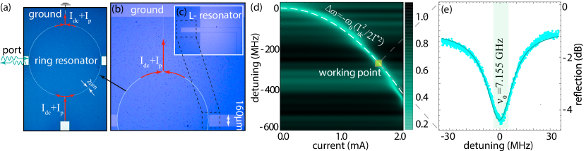
Figure 2: (a) A ring resonator with a $1.3$ mm diameter and a $2\,\mu$m pitch is connected capacitively to an auxiliary resonator. The system is probed through a transmission line connected capacitively to the left side of the ring. A separate line provides the pump and DC current from the device’s bottom, flowing through the ring. (b) Optical image of the KIRPA involving a ring and L-shaped auxiliary resonators. (c) Displays the L-shaped auxiliary resonator with a width of $160\,\mu$m and a length of 4 mm. The design prohibits DC current from passing this resonator, effectively setting the 3WM nonlinearity to zero for the auxiliary resonator. (d) The resonance frequency of the ring resonator as a function of applied bias current. The resonance frequency shows a quadratic pattern with respect to the applied current $\Delta\omega=-\frac{\omega_{0}}{2}\Big{(}\frac{I_{\text{dc}}}{I_{*}}\Big{)}^{2}$. (e) The resonance frequency of the resonator at fixed current $I_{\text{dc}}=1.575$ mA corresponding to $\omega_{0}/2\pi=7.155$ GHz.

III Experimental realization

The amplification process relies on the kinetic inductance exhibited by the superconducting film, which displays a nonlinear dependency on the applied current. This nonlinear behavior can be described by the Ginzburg-Landau theory and the total inductance of the system [51, 52, 45, 53] $L_{k}(I)=L_{0}[1+(\frac{I}{I^{*}})^{2}]$ where $L_{0}$ denotes the kinetic inductance of the film in the absence of current (see Supplementary Materials), while $I^{*}$ is proportional to the critical current of the film and serves as a quantitative gauge of the film’s responsiveness to the applied current $I$.

As shown in Fig. 2a and b, at the core of this amplifier is a ring resonator, used as a nonlinear and dispersive mixing element. The fabrication process involves a straightforward single optical lithography step, as explained in the Supplementary Materials. The resonator is grounded and galvanically connected to both the pump and DC lines. The generated or amplified signal is directed into a waveguide, which is coupled capacitively to the ring resonator. This design simplifies the measurement process and eliminates the requirement for a Bragg mirror or impedance-matching step coupler [35, 36, 37, 38, 39] within the system, resulting in a design that is exceptionally simple and compact. The mixing interaction between idler and signal modes is facilitated by applying a DC current $I_{\text{dc}}$, modifying the circuit inductance

$$L_{k}(I)=L_{0}\Big{[}1+\Big{(}\frac{I_{\text{dc}}}{I_{*}}\Big{)}^{2}+\frac{2I_{\text{rf}}I_{\text{dc}}}{I_{*}^{2}}+\Big{(}\frac{I_{\text{rf}}}{I_{*}}\Big{)}^{2}\Big{]},$$ (13)

where we consider $I=I_{\text{dc}}+I_{\text{rf}}$ in which $I_{\text{rf}}$ is the current of the microwave signal. The first term in Eq. (13) gives the resonance frequency at zero current, whereas the second term characterizes a shift in the resonance frequency of the resonator due to the DC current $\Delta\omega=-\frac{\omega_{0}}{2}\Big{(}\frac{I_{\text{dc}}}{I_{*}}\Big{)}^{2}$. The third term introduces the 3WM process, and finally, the fourth term leads to Kerr nonlinearity [40]. The dependency of the resonance frequency of the mode on the current allows us to extract $I^{*}$ and therefore back out the critical current of the superconducting sheet. Note that the ring resonator in our setup corresponds to resonator $a$ as shown in Figure 1, and it possesses a $\chi^{(2)}$ nonlinearity.

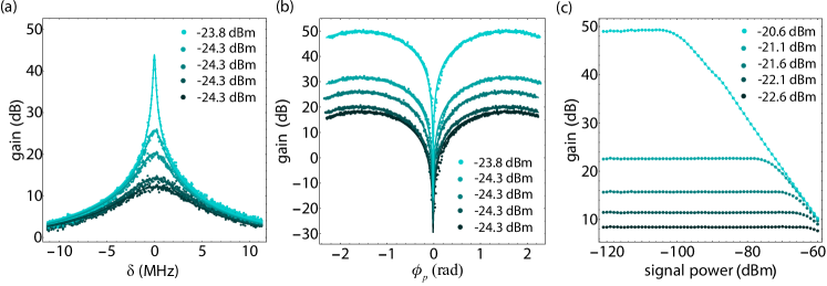
Figure 3: (a) Single-mode phase-insensitive signal gain versus the frequency detuning from the resonator $\omega=\delta+\frac{\omega_{p}}{2}$ for different pump powers. The experimental results (dots) align well with the theoretical model (solid lines) outlined in the text. (b) Phase-sensitive gain as a function of the pump phase $\phi_{p}$. A coherent tone positioned at $\delta=0$ is measured while the pump phase is varied. The data is adjusted to align all dips at zero radians. The result is in good agreement with the theory. (c) The 1-dB compression point for a coherent tone at $\delta=1$ kHz from the amplification center frequency. Power is varied to determine the 1dB compression points at different pump powers.

In addition to the ring resonator, our system also has an auxiliary L-shape resonator (corresponding to resonator $b$ in Fig. 1), which is capacitively coupled to the ring resonator, see Fig. 2b and c. The initial intent behind this setup was to have an additional transmission line for dual-sided probing/measuring of the ring resonator. However, this L-shape section can also act as a large resonator with one end left floating, effectively forming a $\lambda/2$ resonator with a second resonance mode $\omega_{b}$ close to that of the ring resonator $\omega_{a}$. The large size of this auxiliary resonator minimizes its Kerr nonlinearity and allows the handling of substantial power without surpassing the critical current threshold. Moreover, it can be directly wire-bonded, facilitating its utilization as a resonator with significant extrinsic coupling. This capability enables the measurement of the system from an alternative port. The auxiliary resonator is not connected to any DC wires, preventing the flow of biased current through it, thereby maintaining a constant resonance frequency. This setup provides a tunable nonlinear resonator (the ring resonator) connected to a nearby linear auxiliary resonator. This configuration accommodates a pair of coupled modes, initially separated by a spectral gap of approximately $\omega_{a}-\omega_{b}\approx 360$ MHz at zero bias current, as shown in Fig. 4a. By applying a DC current, the frequency of the ring resonator can be adjusted, facilitating the alignment of the two modes at the anticrossing point with an intra-mode coupling strength of $J\approx 21.5$ MHz. As described in the theory section, this coupling plays a critical role in selecting either single or double-mode amplification when the resonances reach the anticrossing point.

To initiate the 3WM process within the system, it is necessary to apply a bias current by utilizing a stable and low noise current source to supply the required current $I_{\mathrm{dc}}$. Subsequently, at the millikelvin stage, this current is combined with the microwave pump, represented as $I_{p}$, through the use of a bias tee. Figure 2d visually demonstrates the influence of the DC current, showing that an increase in the current induces a downward shift in the frequency of the ring resonator that follows the expression $\Delta\omega=-\frac{\omega_{0}}{2}\Big{(}\frac{I_{\text{dc}}}{I^{*}}\Big{)}^{2}$. By precisely knowing the applied current and fitting the frequency shift, we can deduce that $I^{*}=5.86$ mA, a value consistent with previously measured transmission lines of the same width [54] and critical currents of $I_{c}\lesssim 3.91$ mA[40]. Figure 2e shows the system’s reflection from the probe port, demonstrating the resonance frequency of the ring resonator at $\omega_{0}/2\pi=7.155$ GHz for $I_{\text{dc}}=1.575$ mA. Fitting the resonator mode lineshape provides $\kappa_{\text{e}}=19$ MHz and $\kappa_{\text{i}}=4$ MHz, leading to a waveguide-resonator coupling efficiency of $\eta=0.82$. The second mode is not immediately visible from this figure. However, as described in Fig. 4a, upon closer examination or measuring with smaller steps, we can distinctly identify the anticrossing point and the existence of mode $b$.

IV amplification

IV.1 Single-mode amplification

To observe single-mode amplification we choose a bias current $I_{\text{dc}}=1.575$ mA far from the anticrossing point. As a result, we can effectively treat the system as single-mode and Hamiltonian (3) with $g=-I_{\text{dc}}I_{p}\omega_{0}/(4I^{*2})$ [40] can fully describe the amplification process. In this case, the auxiliary resonator will not experience any amplification. We apply a strong pump at a frequency of $\omega_{p}\approx 14.29$ GHz in addition to the bias current $I_{\text{dc}}$ which together results in the down-conversion of pump photons, generating signal and idler photons at $\omega_{p}/2$. Figure 3a shows the non-degenerate gain profile as a function of detuning $\omega=\delta+\frac{\omega_{p}}{2}$ that is measured by sweeping a coherent tone and capturing the maximum gain near half the pump frequency. We observe a substantial gain of approximately 43 dB, achieved with a pump power of $P_{p}=-23.8$ dBm applied at the device’s input. The gain profile is further analyzed using Eq. (II.2), resulting in $\kappa_{\mathrm{e}}=28$ MHz, $\kappa_{\mathrm{i}}=4$ MHz, and the coupling efficiency $\eta=0.9$. A comparison of coupling rates in the presence and absence of pump current shows an increase in the extrinsic coupling rate [40].

Additional amplification can be attained by operating the KIRPA in a degenerate mode, wherein both the signal and idler have the same frequency, $\delta=0$, and exhibit interference based on the phase difference between the pump and the probe $\Delta\phi$. We use a weak probe signal at precisely half the pump frequency and measure the reflection of the system for various phases of the pump, as shown in Fig. 3b. The collected data has been shifted to match $\Delta\phi=0$, where we observe a performance range spanning from $-30$ dB of de-amplification and exceeding $50$ dB of amplification. Employing Eq. (II.2), we once again fit the data, this time centered at $\omega=0$. This analysis also provides insights into the extent of squeezing achievable, as during this operation, it becomes possible to squeeze vacuum fluctuations of one quadrature below the standard quantum limit [55].

Subsequently, we conduct an assessment of the KIRPA’s 1-dB compression point across various pump power levels. This measurement serves to quantify the maximum input power the amplifier can accommodate before reaching saturation. Once again, we apply a probe signal and determine the point at which the KIRPA experiences a 1 dB reduction in its maximum gain by increasing the probe power. The result shows a 1-dB compression power of approximately $-73$ dBm, corresponding to $20$ dB of gain. We note that this compression power is, on average, three orders of magnitude greater than that observed in Josephson-based amplifiers [46].

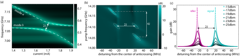
Figure 4: (a) The appearance of the two modes and the anticrossing point as a function of the applied DC current. The two modes are separated by $2J\approx 43$ MHz. (b) Signal amplification versus pump frequency and detuning from the center of the anticrossing. (c) Phase-insensitive gain for the two modes at various pump powers versus the detuning from the center of the anticrossing.

IV.2 Double-mode amplification

As previously discussed, the amplifier design studied here accommodates two modes with an initial spectral separation of approximately $360$ MHz at zero bias current. Nevertheless, by applying a DC current to the ring resonator, we can adjust the resonance frequency and shift it toward the anticrossing points. Note that the appearance of nonlinearity and, subsequently, amplification only happens in the ring resonator. This double-mode system can be effectively described using Eq. (1), where the nonlinear term $a^{2}+a^{\dagger 2}$ is only present in the ring resonator due to applying the biased current and mode $b$ describes the auxiliary resonator (L-shape resonator). Figure 4a shows how the ring resonator, mode $a$, evolves as the bias current is varied, eventually reaching the anticrossing point with the auxiliary resonator with mode $b$.

By aligning the resonance of the two modes and holding them at the anticrossing point, which is achieved by setting $I_{\text{dc}}=1.68$ mA, the system can be operated within the non-degenerate (phase-insensitive) amplification regime described by Hamiltonian (10). Figure 4b shows the amplification versus the detuning from the anticrossing point and the pump frequency $\omega_{p}$. There are three distinct amplification regimes evident in this figure. In the initial region, when $\Delta\approx-J$, single-mode amplification is observed around $\omega_{p}\approx 14.059$ GHz, corresponding to the term $c^{2}_{-}$ in Hamiltonian (10). The second region indicates double-mode amplification or the activation of $c_{-}c_{+}$ terms at $\Delta\approx 0$, which is represented by the presence of two peaks at $\omega_{p}\approx 14.1$ GHz well-separated by $2J$. In the third regime, amplification at $\omega_{p}\approx 14.15$ GHz occurs when $\Delta\approx J$, corresponding to the term $c^{2}_{+}$. Note that, the pump frequency separation between the first and last regimes, $\delta_{p}\approx 91$ MHz, is determined by the coupling strength between the two modes $\delta_{p}\approx 4J$, as anticipated. Figure 4 c demonstrates double-mode (non-degenerate) amplification for different pump powers at $\Delta\approx 0$. It shows the amplification of the signal and idler modes achieving up to $32$ dB gain in both modes. The experimental results align well with our comprehensive theoretical model.

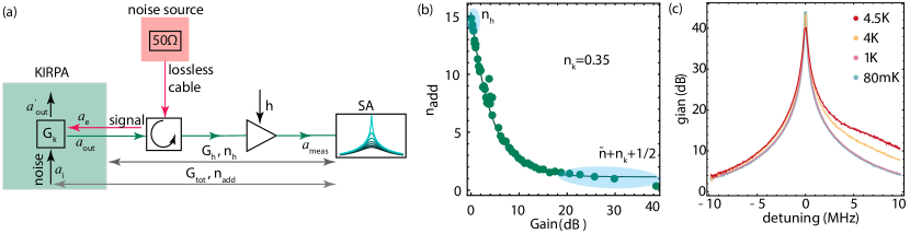
Figure 5: (a) The illustration of the noise calibration setup. A $50\,\Omega$-terminator, varied in temperature, acts as the known noise source. The generated noise is directed to the KIRPA at varying gains. By utilizing the Bose-Einstein distribution to fit the noise spectrum, we extract the total gain and quanta noise added by the amplification chain. (b) The noise quanta added by the whole amplification chain versus the gain of the KIRPA. At zero gain ($G_{\text{k}}=0$), the noise of the classical amplification chain $n_{\text{h}}$ dominates the added noise. In contrast, at large gains ($G_{\text{k}}\gg 1$), the noise added by the KIRPA becomes noticeable $n_{\text{add}}\approx(\bar{n}+\frac{1}{2}+n_{\text{k}})$. Fitting the data using the theoretical model results in $n_{\text{k}}\approx 0.35$. (c) A comparison of the KIRPA gain at different device temperatures ($80$ mK, $1$ K, $4$ K, and $4.5$ K) is presented.

V Noise Characterization and Effect of Operating Temperature

Another important aspect of a parametric amplifier is its noise behavior. We examine the noise performance of the KIRPA in the single-mode regime by evaluating a chain of amplifiers and determining the additional noise introduced by the KIRPA, as illustrated in Fig. 5a. The output chain is divided into two parts: the KIRPA, with gain $G_{\text{k}}$ and input-referred added noise $n_{\text{k}}$, and the classical amplification chain consisting of gain $G_{\text{h}}$ and noise quanta $n_{\text{h}}$. This classical chain represents the collective gain and noise arising from the HEMT (near 4K), the low noise amplifier (at room temperature), and the cable losses across the chain. Near the non-degenerate amplification regime, the field operator describing the entire chain is given by

$$a_{\text{meas}}=\sqrt{G_{\text{h}}}a_{\text{out}}+\sqrt{G_{\text{h}}-1}h^{\dagger},$$ (14)

where $h$ represents the noise operator introduced by the classical amplification chain following the KIRPA, while $a_{\text{out}}$ characterizes the KIRPA’s output. By utilizing the above equation, the total noise quanta of the entire amplification chain can be computed (see the Supplementary Materials for further details)

$$N_{\text{tot}}\approx G_{\text{tot}}\Big{[}\frac{1}{2}\,\text{coth}\big{(}\frac{\hbar\omega}{2k_{B}T}\big{)}+n_{\text{add}}\Big{]}$$ (15)

where $G_{\text{tot}}=G_{\text{h}}G_{\text{k}}$ is the total gain and

$$n_{\text{add}}=\frac{G_{\text{k}}-1}{G_{\text{k}}}\Big{(}\bar{n}+\frac{1}{2}+n_{\text{k}}\Big{)}+\frac{n_{\text{h}}}{G_{\text{k}}},$$ (16)

is the total input-referred noise of the amplification chain. Here, $\bar{n}(T)=(e^{\hbar\omega/k_{B}T}-1)^{-1}$ is the thermal noise at temperature $T$, $k_{B}$ is the Boltzmann constant, and

$$n_{\text{k}}=\Big{(}\frac{1-\eta}{\eta}\Big{)}\Big{[}2\bar{n}(T_{\text{dev}})+1\Big{]},$$ (17)

is the input-referred noise added by the KIRPA at a given device temperature $T_{\text{dev}}$. In perfect coupling regime $\eta\approx 1$, a very low temperature $\bar{n}\approx 0$, and at the large gain $G_{\text{k}}\gg 1$ such that $\frac{n_{\text{h}}}{G_{\text{k}}}\approx 0$, the total noise of the amplifier reduces to the vacuum noise $n_{\text{add}}\approx\frac{1}{2}$, as anticipated for an ideal non-degenerate quantum-limited amplifier.

By generating a known noise using a temperature-controlled $50\,\Omega$ load noise source and feeding it into the KIRPA, we estimate the overall device noise at various gains, see Fig. 5a. First, during the noise calibration with the pump off, we deduce the gain $G_{\text{h}}$ and added noise $n_{\text{h}}$ of the classical amplification chain. Next, with the pump turned on, we measure the system’s noise to determine $G_{\text{k}}$ and $n_{\text{add}}$, as shown in Fig. 5b. We use Eq. (16) to fit the experimental result, yielding $n_{\text{k}}\approx 0.35$ at around $230$ mK, a close match to the theoretical estimation obtained from Eq. (17) of $n_{\text{k}}\approx 0.39$ quanta noise. In Figure 5b for small KIRPA gains ($G_{\text{k}}\approx 0$), the noise from the classical amplification chain becomes the main source of noise i.e. $n_{\text{add}}=n_{\text{h}}$. Conversely, at significantly high gains, the KIRPA noise dominates the overall system noise $n_{\text{add}}\approx(\bar{n}+\frac{1}{2}+n_{\text{k}})$.

As a final remark, we describe the operational performance of our device at different temperatures. The kinetic inductance properties of KIRPA, along with its independence from Josephson junctions, offer a substantial advantage when it comes to operating it at higher temperatures [56], a limitation that affects JPA and JTWP devices. We can test and operate the amplifier at different temperatures and measure the gain at different phases of the process. In Fig. 5c, the gain of the amplifier in the single mode is illustrated at various device temperatures. It is apparent that the amplifier effectively maintains its gain performance, even at temperatures reaching up to 4.5 K. However, due to technical limitations and the inability to regulate the dilution refrigerator’s temperature beyond 4.5 K, evaluating the device’s performance at higher temperatures was unattainable.

VI Conclusion and Discussions

In summary, we have developed a junction-free quantum-limited amplifier based on kinetic inductance superconductivity. The design of our amplifier is inherently simple and does not necessitate complex circuitry or impedance-matching step couplers for amplification generation [40]. Overcoming the limitations of conventional Josephson junction amplifiers, this device operates at temperatures above 4.5 K. Its double-mode capability, tunability through bias current, facilitates selective operation in both single and double-mode amplification regimes, achieving gains surpassing 50 dB in single-mode and 32 dB in double-mode configurations while only adding $0.35$ quanta noise. Compared to Josephson junction-based amplifiers our device presents a remarkably improved 1 dB compression point of $-73$ dB at $20$ dB gain mainly due to the small contribution of the self-Kerr term in the system. Additionally, using niobium titanium nitride offers resilience against magnetic fields, up to 2 T [47, 42].

This amplifier can potentially be used in a broad range of quantum applications, particularly in the domain of quantum computing. Its adaptability and resilience make it a fitting candidate for integration into future superconducting quantum computers, enhancing microwave measurements and enabling fast and accurate readout of superconducting qubits and spins. Additionally, its ability to perform effectively at higher temperatures suggests its utility in quantum sensing and reading applications, such as quantum illumination and radar [31]. Moreover, its resilience to magnetic fields opens possibilities for integration into hybrid quantum circuits or for the readout of spins and colored centers that necessitate magnetic fields for their control.

The low loss of our sample enables the generation of nonclassical radiation, such as entanglement and squeezing within the circuit. Quantum entanglement finds applications in quantum sensing, linking remote quantum nodes, and establishing entangled clusters across a chip. Squeezing, however, is a valuable resource for universal quantum computing [57, 58]. The simple design, high fabrication yield, minimal loss, and scalability of our device could potentially find applications in microwave continuous variable quantum computing [59].

Acknowledgments We thank Joe Salfi, Leonid Belostotski, and Mohammad Khalifa helpful comments and discussions. S.B. acknowledges funding by the Natural Sciences and Engineering Research Council of Canada (NSERC) through its Discovery Grant and Quantum Alliance Grant, funding and advisory support provided by Alberta Innovates (AI) through the Accelerating Innovations into CarE (AICE) – Concepts Program, support from Alberta Innovates and NSERC through Advance Grant project, and Alliance Quantum Consortium. This project is funded [in part] by the Government of Canada. Ce projet est financé [en partie] par le gouvernement du Canada.

Supplementary Materials

.1 Measurement setup

A bias tee is used to combine dc current $I_{\text{dc}}$ and pump $I_{p}$ at the mixing chamber of the dilution refrigerator, as seen in Fig. 6. The output of the bias tee is directly connected to KIRPA. Applying a biased current leads to a shift in the resonance frequency, as explained in the main text. This shift allows us to infer $I^{*}$. Consequently, we select $I_{\text{dc}}$ to maximize the ratio $I_{\text{dc}}/I^{*}$ while remaining far from the sheet’s critical current $I_{\text{c}}$. This allows having enough room to not break superconductivity by applying the pump to the system. By introducing a pump and sweeping its frequency, we can identify the optimal amplification point. This measurement is conducted using either a Vector Network Analyzer (VNA) or a Spectrum Analyzer (SA).

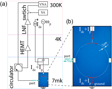
Figure 6: (a) A schematic representation of the measurement setup for our device. A bias tee mixes the DC and pump current and is supplied to the KIRPA galvanically. The attenuated input signal is sent to the device and then directed to a HEMT at 4K and room temperature amplifier (LNF) at 300K and is measured by either a spectrum analyzer (SA) or vector network analyzer (VNA). (b) The KIRPA is a $1300\,\mu$m diameter ring resonator with a $2\,\mu$m pitch, capacitively connected to an L-shaped resonator. The system is probed via a transmission line, capacitively connected to the left side of the ring. An additional line supplies the pump and DC current from the device’s top, flowing to the ground through the ring.

For probe amplification, we utilized the VNA (Rohde and Schwarz ZBN20) and aligned the center frequency of the VNA trace to half of the pump frequency. By sweeping the pump frequency and measuring with the VNA, we can capture the maximum gain at various DC currents. The assessment of noise amplification was conducted using an SA (Rohde and Schwarz FSW), where the output power spectral density enables the measurement of vacuum noise amplification within the KIRPA. This particular measurement allows for the determination of the noise added by the KIRPA during the amplification process.

.2 System Noise calibration

We determine the system gain $G$ and the system noise $n_{\text{add}}$ for both the HEMT and KIRPA by introducing a known quantity of thermal noise using temperature-controlled $50\,\Omega$ load. By varying the temperature of the $50\,\Omega$ load and recording its temperature, we can generate predictable thermal noises. These noises will serve the purpose of calibrating the measurement chain. The calibration devices are connected to the measurement setup via two 5-cm-long superconducting coaxial cables and a thin copper braid (providing weak thermal anchoring to the mixing chamber plate) using a latching microwave switch (Radiall R573423600). By measuring the noise density (in square volts per hertz) at different temperatures and fitting the collected data with the anticipated scaling,

$$N_{\text{tot}}=G_{\text{tot}}\hbar\omega\Big{[}\frac{1}{2}\text{coth}\Big{(}\frac{\hbar\omega}{2k_{B}T}\Big{)}+n_{\text{add}}\Big{]},$$ (18)

we accurately determine the gain $G_{\text{tot}}$ and the added noise photons $n_{\text{add}}$ for each section of the amplification chain.

.3 Sample Design

The primary aim in designing our amplifier is to have a well-defined resonance that could be consistently measured and tracked while adjusting the frequency to targeted regions. To achieve this, we opted for a ring resonator that is capacitively coupled to a coplanar waveguide (CPW) transmission line. The ring is grounded to supply DC and pump current, effectively forming $\lambda$/4 resonator. While the aforementioned setup can enable single-mode amplification, we introduced an additional L-shaped resonator to generate double-mode amplification by capacitively coupling it to the ring using a coupling rate $J$.

The ring resonator itself resonates at a frequency of $7.4$ GHz at zero dc-current. Its specific dimensions, including a radius of $650\,\mu$m and a track width of $2\,\mu$m, were determined through simulations conducted in Sonnet. The resonator’s width was adjusted to minimize Kerr effects.

The auxiliary resonator is designed in an L-shaped structure with a specific width of $160\,\mu$m and length of $4$ mm. Its considerable size offers two notable advantages. First, it facilitates direct wire bonding to the input port on the hosting PCB, serving as a port for measurements or probing within the system. By employing the cryogenic switch and connecting this resonator to it, we can even directly measure the system’s reflection. Second, it can be considered as a linear resonator with a second resonance frequency closer to the ring resonator. An interesting aspect of this design is that, when the transmission port (connected to this resonator via the cryogenic switch) is closed, and the resonator is left floating, the L-shaped auxiliary resonator effectively functions as a $\lambda/2$ resonator capable of coupling with the ring resonator. The first resonance mode of this resonator occurs at around $4.4$ GHz, while the second resonance mode is at $7.03$ GHz. However, when the switch is open and connected to the L-shaped resonator, its extrinsic coupling $\kappa_{\text{e}}$ becomes significantly large, resulting in an extremely flattened mode that is not easily observable in the anticrossing points, as seen in Fig. 7.

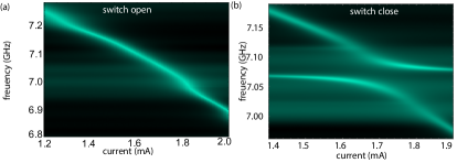
Figure 7: (a) The system’s reflection is plotted against the applied dc-current in the presence of the cryogenic switch connected to the auxiliary resonator. This configuration results in a very large extrinsic coupling rate, causing the anticrossing point to be obscured. (b) A close-up view of the anticrossing point after disconnecting the cryogenic switch from the L-shaped resonator. In this configuration, the anticrossing point becomes distinctly visible.

.4 Change in extrinsic and intrinsic couplings

As previously discussed, the variability in both extrinsic and intrinsic coupling rates is anticipated due to the dependence of kinetic inductance on the RF current applied to the device. Figure 8 illustrates the variations in both $\kappa_{e}$ and $\kappa_{i}$ for the ring-resonator as the pump power to the device is increased. The precise determination of pump current is challenging due to the unknown impedance of the device. Nonetheless, a noticeable trend emerges, showing that an increase in pump power corresponds to an increase in coupling rates. The rise in $\kappa_{e}$ is influenced by its dependence on inductance, typically a constant determined solely by the device’s geometry. However, in our case, the kinetic inductance, which significantly is bigger than the geometric inductance, dominates the total inductance, impacting $\kappa_{e}$. The increase in $\kappa_{i}$ is attributed to impurities and defects in the device fabrication, leading to an increase in $\kappa_{i}$ when stimulated by current.

Figure 8: (a) The extrinsic $\kappa_{e}$ and (b) intrinsic coupling rate at different pump powers, extracted by fitting different amplification profiles.

.5 Gain-Bandwidth product

Subsequently, we proceed to extract the bandwidth and gain bandwidth product (GBP) at different gains. Bandwidth (BW) is defined as the full half-width maximum of linear gain, and GBP is defined as $\sqrt{G_{\text{lin}}}*BW$. Measured linear gain data is fitted to a Lorentzian line shape to extract the bandwidth. For sufficiently large gains, we anticipate GBP to be on the order of $\kappa_{e}$ as confirmed in Fig. 9.

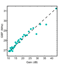
Figure 9: Gain bandwidth product (GBP) at different gains of the KIRPA.

.6 Kinetic Inductance

The total kinetic inductance of both resonators, $L_{0}$, is determined by the sheet inductance of the thin film, which varies based on the film’s thickness. We deduce the sheet inductance $L_{\square}$ by analyzing the resonance frequency of the ring resonator at zero bias current. Utilizing simulations in Sonnet and adjusting the sheet inductance to align with the experimental result, we can infer the sheet inductance of the film, resulting in the value of $L_{\square}=30$ pH. This analysis assumes a uniformly evaporated film across the entire chip. The total inductance corresponding to this sheet inductance then will be $L_{0}=251$ nH.

.7 Sample Fabrication

The fabrication process involves a straightforward single lithographic step facilitated by an optical lithographer. Initially, a silicon wafer with a thickness of 500 um is coated with a $10$ nm layer of NbTiN and diced into smaller chips. The fabrication procedure starts with a cleaning step involving Acetone and IPA, where the chip is subjected to a 5-minute sonication treatment in each solution. The chip’s surface is subsequently coated with AZ 1529 resist followed by the Optical Lithography step to pattern the design. The final step involves etching the device using an ICP Reactive Ion Etcher. Subsequently, the device is wire bonded onto a printed circuit board (PCB), which is then affixed to a copper enclosure destined for placement within a dilution refrigerator.

.8 Theory of the single-mode (degenerate) amplification

The Hamiltonian describing a single mode resonator containing $\chi^{(2)}$ nonlinearity is given by

$$H=\omega_{a}a^{\dagger}a+\frac{g_{0}}{2}(a^{2}a_{p}^{\dagger}+a^{\dagger 2}a_{p}),$$ (19)

where the second term describes the Three-Wave-Mixing (3WM) process, where a pump photon at frequency $\omega_{p}$ is eliminated, producing two photons at the resonance frequency $\omega_{a}$. Thus, the conservation of energy dictates $\omega_{p}=2\omega_{a}$.

In the strong pump regime, we can ignore the field fluctuations and the pump can be treated as a classical field with the amplitude $a_{p}\rightarrow\alpha_{p}=|\alpha_{p}|e^{-i\phi_{p}}e^{-i\omega_{p}t}$. A critical point to highlight is that if this approximation does not hold, our amplifier would not satisfy the linear amplification criteria we are aiming for. By using this approximation, we can subsequently simplify our analysis by neglecting the dynamics of the pump degree of freedom and focusing on the reduced system Hamiltonian

$$H=\Delta a^{\dagger}a+\frac{g}{2}(a^{2}+a^{\dagger 2}),$$ (20)

where $g=g_{0}|\alpha_{p}|$ and $\phi_{p}$ is the global phase set by the pump. The above Hamiltonian has been written in a reference frame rotating at $\omega_{p}/2=\omega_{a}-\Delta$.

The complete quantum description of the system can be expressed using the quantum Langevin equations. These equations incorporate quantum noise affecting input fluctuations for the resonator ($a_{\mathrm{e}}$ with extrinsic damping rate $\kappa_{\mathrm{e}}$) and the intrinsic losses in the resonator mode ($a_{\mathrm{i}}$ with intrinsic damping rate $\kappa_{\mathrm{i}}$). The correlations for these noises are defined as follows:

$$\langle a_{\mathrm{e(i)}}(t)a_{\mathrm{e(i)}}^{\dagger}(t^{\prime})\rangle = \langle a_{\mathrm{e(i)}}^{\dagger}(t)a_{\mathrm{e(i)}}(t^{\prime})\rangle+\delta(t-t^{\prime})$$ (21)

$$= (\bar{n}_{\mathrm{e(i)}}+1)\delta(t-t^{\prime}),$$

where $\delta(t)$ is the Dirac delta function and $\bar{n}_{\mathrm{e(i)}}$ are the Planck-law thermal occupancies of microwave mode (bath). The resulting Langevin equations corresponding to Hamiltonian (20) are

$$\dot{a} = -\Big{(}i\Delta+\frac{\kappa}{2}\Big{)}a-ige^{i\phi_{p}}a^{\dagger}+\sqrt{\kappa_{\mathrm{e}}}a_{\mathrm{e}}+\sqrt{\kappa_{\mathrm{i}}}a_{\mathrm{i}},$$

$$\dot{a}^{\dagger} = \Big{(}i\Delta-\frac{\kappa}{2}\Big{)}a^{\dagger}+ige^{-i\phi_{p}}a+\sqrt{\kappa_{\mathrm{e}}}a_{\mathrm{e}}^{\dagger}+\sqrt{\kappa_{\mathrm{i}}}a_{\mathrm{i}}^{\dagger},$$ (22)

where $\kappa=\kappa_{\mathrm{e}}+\kappa_{\mathrm{i}}$ is the total damping rate of the resonator. We can solve the above equations in the Fourier domain to obtain the intra-cavity operator $a$. By substituting the solutions of Eqs. (22) into the corresponding input-output relation i.e., $a_{\mathrm{out}}=\sqrt{\kappa_{\mathrm{e}}}a-a_{\mathrm{in}}$, we obtain

$$\textbf{S}_{\mathrm{out}}(\omega)=\textbf{M}(\omega)\textbf{S}_{\mathrm{in}}(\omega)$$ (23)

where $\textbf{S}_{\mathrm{out}}=[a_{\mathrm{out}},a_{\mathrm{out}}^{\dagger}]^{\textbf{T}}$, $\textbf{M}(\omega)=\Big{(}\textbf{C}.[\textbf{A}]^{-1}.\textbf{B}-\textbf{D}\Big{)}$ with I is the identity matrix, and $\textbf{S}_{\mathrm{in}}=[a_{\mathrm{e}},a_{\mathrm{i}},a_{\mathrm{e}}^{\dagger},a_{\mathrm{i}}^{\dagger}]^{\textbf{T}}$, and we defined the following matrices

$$\textbf{A}=-i\omega\textbf{I}-\begin{bmatrix}-\Big{(}i\Delta+\frac{\kappa}{2}\Big{)}&-ige^{i\phi_{p}}\\ ige^{-i\phi_{p}}&\Big{(}i\Delta-\frac{\kappa}{2}\Big{)}\end{bmatrix},$$ (24)

$$\textbf{B}=\begin{bmatrix}\sqrt{\kappa_{\mathrm{e}}}&\sqrt{\kappa_{\mathrm{i}}}&0&0\\ 0&0&\sqrt{\kappa_{\mathrm{e}}}&\sqrt{\kappa_{\mathrm{i}}}\end{bmatrix},\textbf{D}=\begin{bmatrix}1&0&0&0\\ 0&0&1&0\end{bmatrix}$$ (25)

and $\textbf{C}=\sqrt{\kappa_{\mathrm{e}}}\textbf{I}$. Note that the inverse of the matrix A at $\Delta=0$ gives the susceptibility of the resonator $\bm{\chi}(\omega)=\textbf{A}^{-1}$. The total output field then has the following form

$$a_{\mathrm{out}}(\omega)=\Big{[}\mathcal{G}_{S}(\omega)a_{\text{e}}+\mathcal{G}_{I}(\omega)a_{\text{e}}^{\dagger}\Big{]}+\sqrt{\frac{1-\eta}{\eta}}\Big{[}(\mathcal{G}_{S}(\omega)+1)a_{\text{i}}+\mathcal{G}_{I}(\omega)a_{\text{i}}^{\dagger}\Big{]}$$ (26)

where $\eta=\frac{\kappa_{\text{e}}}{\kappa}$ describes the waveguide-resonator coupling and we define

$$\mathcal{G}_{S}(\omega) = \frac{\eta\kappa\Big{[}\frac{\kappa}{2}-i(\omega+\Delta)\Big{]}}{\Delta^{2}-g^{2}+(i\omega-\frac{\kappa}{2})^{2}}+1,$$

$$\mathcal{G}_{I}(\omega) = \frac{i\eta\kappa ge^{i\phi}}{\Delta^{2}-g^{2}+(i\omega-\frac{\kappa}{2})^{2}}.$$ (27)

The linear amplification model being analyzed here must hold the bosonic commutation relation for the output field operator $[a_{\mathrm{out}}(\omega),a_{\mathrm{out}}^{\dagger}(\omega^{\prime})]=\delta(\omega-\omega^{\prime})$, and thus

$$|\mathcal{G}_{I}|^{2}\Big{(}1+\frac{1-\eta}{\eta}\Big{)}=|\mathcal{G}_{S}|^{2}+\Big{(}\frac{1-\eta}{\eta}\Big{)}|\mathcal{G}_{S}+1|^{2}-1,$$ (28)

where for a lossless resonator ($\eta=1$) we get $|\mathcal{G}_{I}|^{2}=|\mathcal{G}_{S}|^{2}-1$, as presented in the main text.

.9 Theory of the added noise

In this section, we present the theoretical model of the added noise within the amplification chain. The input signal traverses through the KIRPA, and then undergoes propagation via transmission cables before being amplified by an HEMT at the 4K stage and a subsequent amplifier at room temperature. Here, the gain of the KIRPA is given by $G_{\text{k}}=|\mathcal{G}_{s}|^{2}$, while $G_{\text{h}}$ represents the collective noise of both the HEMT and the room-temperature amplifier, containing all losses occurring in the cables between the calibration tool and the Spectrum Analyzer at room temperature.

The output of the KIRPA when operating in the nondegenerate parametric regime is given by Eq. (26). The signal then passes through the amplification chain leading to

$$a_{\text{meas}}=\sqrt{G_{\text{h}}}a_{\text{out}}+\sqrt{G_{\text{h}}-1}h^{\dagger},$$ (29)

where $h$ is the noise operator added by the amplification chain after the KIRPA. The total noise quanta can be calculated using the measured spectrum of the system at a given bandwidth $BW$

$$\frac{S_{\text{meas}}}{BW}=\hbar\omega\Big{(}\frac{\langle\Delta I_{\text{meas}}^{2}\rangle+\langle\Delta Q_{\text{meas}}^{2}\rangle}{2}\Big{)}$$ (30)

where $I_{\text{meas}}=\frac{a_{\text{meas}}+a_{\text{meas}}}{\sqrt{2}}$ and $Q_{\text{meas}}=\frac{a_{\text{meas}}-a_{\text{meas}}}{i\sqrt{2}}$ are the quadrature operators. Therefore the total noise quanta is given by

$$N_{\text{tot}}=\frac{S_{\text{meas}}}{BW} = \frac{1}{2}\hbar\omega G_{\text{h}}\Big{[}|\mathcal{G}_{S}(\omega)|^{2}(2\bar{n}(T)+1)+|\mathcal{G}_{I}(\omega)|^{2}(2\bar{n}(T)+1)+\Big{(}\frac{1-\eta}{\eta}\Big{)}\Big{(}|\mathcal{G}_{S}(\omega)+1|^{2}+|\mathcal{G}_{I}(\omega)|^{2}\Big{)}(2\bar{n}(T)+1)$$ (31)

$$+ \frac{G_{\text{h}}-1}{G_{\text{h}}}n_{\text{h}}\Big{]},$$

where $\bar{n}(T)=(e^{\hbar\omega/k_{B}T}-1)^{-1}$ is thermal noise and $n_{\text{h}}=2\langle h^{\dagger}h\rangle+1$ is the noise added by the amplification chain after the KIRPA. In the large gain regime $\frac{G_{\text{h}}-1}{G_{\text{h}}}\approx 1$ the above expression can be written as

$$N_{\text{tot}}\approx G_{\text{tot}}\hbar\omega\Big{[}0.5\,\text{coth}\big{(}\frac{\hbar\omega}{2k_{B}T}\big{)}+n_{\text{add}}\Big{]}$$ (32)

where $G_{\text{tot}}=G_{\text{h}}G_{\text{k}}$ is the total gain of the chain and

$$n_{\text{add}}=\frac{G_{\text{k}}-1}{G_{\text{k}}}\Big{(}\bar{n}+\frac{1}{2}+n_{\text{k}}\Big{)}+\frac{n_{\text{h}}}{G_{\text{k}}},$$ (33)

is the total input-referred noise added by the amplification chain. The first two terms illustrate the noise added by an ideal non-degenerate amplifier, while the last term demonstrates the noise added by the amplification chain, excluding the KIRPA. The input-referred noise contribution of the KIPA in nondegenerate mode is given by

$$n_{\text{k}}=\Big{(}\frac{1-\eta}{\eta}\Big{)}\frac{(\sqrt{G_{\text{k}}}+1)^{2}}{G_{\text{k}}-1}\Big{[}2\bar{n}+1\Big{]},$$ (34)

where we assume $\mathcal{G}_{s}$ is real. For large gain $G_{\text{k}}\gg 1$, the above expression reduces to

$$n_{\text{k}}=\Big{(}\frac{1-\eta}{\eta}\Big{)}\Big{[}2\bar{n}+1\Big{]},$$ (35)

as presented in the main text. It is obvious that for a near ideal resonator $\eta\rightarrow 1$, the total noise of the amplification chain reduces to the noise expression for an ideal non-degenerate amplifier (for $G_{\text{k}}\gg 1$)

$$n_{\text{add}}\approx\bar{n}+\frac{1}{2}$$ (36)

References

- Caves [1982] C. M. Caves, Quantum limits on noise in linear amplifiers, Phys. Rev. D 26, 1817 (1982).
- Clerk et al. [2010] A. A. Clerk, M. H. Devoret, S. M. Girvin, F. Marquardt, and R. J. Schoelkopf, Introduction to quantum noise, measurement, and amplification, Rev. Mod. Phys. 82, 1155 (2010).
- Aumentado [2020a] J. Aumentado, Superconducting parametric amplifiers: The state of the art in josephson parametric amplifiers, IEEE Microwave Magazine 21, 45 (2020a).
- Blais et al. [2021] A. Blais, A. L. Grimsmo, S. M. Girvin, and A. Wallraff, Circuit quantum electrodynamics, Rev. Mod. Phys. 93, 025005 (2021).
- Castellanos-Beltran and Lehnert [2007] M. A. Castellanos-Beltran and K. W. Lehnert, Widely tunable parametric amplifier based on a superconducting quantum interference device array resonator, Applied Physics Letters 91, 083509 (2007), https://pubs.aip.org/aip/apl/article-pdf/doi/10.1063/1.2773988/13979299/083509_1_online.pdf .
- Hatridge et al. [2011] M. Hatridge, R. Vijay, D. H. Slichter, J. Clarke, and I. Siddiqi, Dispersive magnetometry with a quantum limited squid parametric amplifier, Phys. Rev. B 83, 134501 (2011).
- Bergeal et al. [2010] N. Bergeal, F. Schackert, M. Metcalfe, R. Vijay, V. E. Manucharyan, L. Frunzio, D. E. Prober, R. J. Schoelkopf, S. M. Girvin, and M. H. Devoret, Phase-preserving amplification near the quantum limit with a josephson ring modulator, Nature 465, 64 (2010).
- Macklin et al. [2015] C. Macklin, K. O’Brien, D. Hover, M. E. Schwartz, V. Bolkhovsky, X. Zhang, W. D. Oliver, and I. Siddiqi, A near–quantum-limited josephson traveling-wave parametric amplifier, Science 350, 307 (2015), https://www.science.org/doi/pdf/10.1126/science.aaa8525 .
- Aumentado [2020b] J. Aumentado, Superconducting parametric amplifiers: The state of the art in josephson parametric amplifiers, IEEE Microwave Magazine 21, 45 (2020b).
- Esposito et al. [2021a] M. Esposito, A. Ranadive, L. Planat, and N. Roch, Perspective on traveling wave microwave parametric amplifiers, Applied Physics Letters 119, 120501 (2021a), https://pubs.aip.org/aip/apl/article-pdf/doi/10.1063/5.0064892/13282980/120501_1_online.pdf .
- Walter et al. [2017] T. Walter, P. Kurpiers, S. Gasparinetti, P. Magnard, A. Potočnik, Y. Salathé, M. Pechal, M. Mondal, M. Oppliger, C. Eichler, and A. Wallraff, Rapid high-fidelity single-shot dispersive readout of superconducting qubits, Phys. Rev. Appl. 7, 054020 (2017).
- Heinsoo et al. [2018] J. Heinsoo, C. K. Andersen, A. Remm, S. Krinner, T. Walter, Y. Salathé, S. Gasparinetti, J.-C. Besse, A. Potočnik, A. Wallraff, and C. Eichler, Rapid high-fidelity multiplexed readout of superconducting qubits, Phys. Rev. Appl. 10, 034040 (2018).
- Vijay et al. [2011] R. Vijay, D. H. Slichter, and I. Siddiqi, Observation of quantum jumps in a superconducting artificial atom, Phys. Rev. Lett. 106, 110502 (2011).
- Jeffrey et al. [2014] E. Jeffrey, D. Sank, J. Y. Mutus, T. C. White, J. Kelly, R. Barends, Y. Chen, Z. Chen, B. Chiaro, A. Dunsworth, A. Megrant, P. J. J. O’Malley, C. Neill, P. Roushan, A. Vainsencher, J. Wenner, A. N. Cleland, and J. M. Martinis, Fast accurate state measurement with superconducting qubits, Phys. Rev. Lett. 112, 190504 (2014).
- Vine et al. [2023] W. Vine, M. Savytskyi, A. Vaartjes, A. Kringhøj, D. Parker, J. Slack-Smith, T. Schenkel, K. Mølmer, J. C. McCallum, B. C. Johnson, A. Morello, and J. J. Pla, In situ amplification of spin echoes within a kinetic inductance parametric amplifier, Science Advances 9, eadg1593 (2023), https://www.science.org/doi/pdf/10.1126/sciadv.adg1593 .
- Schaal et al. [2020] S. Schaal, I. Ahmed, J. A. Haigh, L. Hutin, B. Bertrand, S. Barraud, M. Vinet, C.-M. Lee, N. Stelmashenko, J. W. A. Robinson, J. Y. Qiu, S. Hacohen-Gourgy, I. Siddiqi, M. F. Gonzalez-Zalba, and J. J. L. Morton, Fast gate-based readout of silicon quantum dots using josephson parametric amplification, Phys. Rev. Lett. 124, 067701 (2020).
- Stehlik et al. [2015] J. Stehlik, Y.-Y. Liu, C. M. Quintana, C. Eichler, T. R. Hartke, and J. R. Petta, Fast charge sensing of a cavity-coupled double quantum dot using a josephson parametric amplifier, Phys. Rev. Appl. 4, 014018 (2015).
- Kerckhoff et al. [2013] J. Kerckhoff, R. W. Andrews, H. S. Ku, W. F. Kindel, K. Cicak, R. W. Simmonds, and K. W. Lehnert, Tunable coupling to a mechanical oscillator circuit using a coherent feedback network, Phys. Rev. X 3, 021013 (2013).
- Castellanos-Beltran et al. [2008] M. A. Castellanos-Beltran, K. D. Irwin, G. C. Hilton, L. R. Vale, and K. W. Lehnert, Amplification and squeezing of quantum noise with a tunable josephson metamaterial, Nature Physics 4, 929 (2008).
- Fedorov et al. [2016] K. G. Fedorov, L. Zhong, S. Pogorzalek, P. Eder, M. Fischer, J. Goetz, E. Xie, F. Wulschner, K. Inomata, T. Yamamoto, Y. Nakamura, R. Di Candia, U. Las Heras, M. Sanz, E. Solano, E. P. Menzel, F. Deppe, A. Marx, and R. Gross, Displacement of propagating squeezed microwave states, Phys. Rev. Lett. 117, 020502 (2016).
- Mallet et al. [2011] F. Mallet, M. A. Castellanos-Beltran, H. S. Ku, S. Glancy, E. Knill, K. D. Irwin, G. C. Hilton, L. R. Vale, and K. W. Lehnert, Quantum state tomography of an itinerant squeezed microwave field, Phys. Rev. Lett. 106, 220502 (2011).
- Murch et al. [2013] K. W. Murch, S. J. Weber, C. Macklin, and I. Siddiqi, Observing single quantum trajectories of a superconducting quantum bit, Nature 502, 211 (2013).
- Weber et al. [2014] S. J. Weber, A. Chantasri, J. Dressel, A. N. Jordan, K. W. Murch, and I. Siddiqi, Mapping the optimal route between two quantum states, Nature 511, 570 (2014).
- Caldwell et al. [2017] A. Caldwell, G. Dvali, B. Majorovits, A. Millar, G. Raffelt, J. Redondo, O. Reimann, F. Simon, and F. Steffen (MADMAX Working Group), Dielectric haloscopes: A new way to detect axion dark matter, Phys. Rev. Lett. 118, 091801 (2017).
- Jeong et al. [2020] J. Jeong, S. Youn, S. Bae, J. Kim, T. Seong, J. E. Kim, and Y. K. Semertzidis, Search for invisible axion dark matter with a multiple-cell haloscope, Phys. Rev. Lett. 125, 221302 (2020).
- Wurtz et al. [2021] K. Wurtz, B. Brubaker, Y. Jiang, E. Ruddy, D. Palken, and K. Lehnert, Cavity entanglement and state swapping to accelerate the search for axion dark matter, PRX Quantum 2, 040350 (2021).
- Backes et al. [2021] K. M. Backes, D. A. Palken, S. A. Kenany, B. M. Brubaker, S. B. Cahn, A. Droster, G. C. Hilton, S. Ghosh, H. Jackson, S. K. Lamoreaux, A. F. Leder, K. W. Lehnert, S. M. Lewis, M. Malnou, R. H. Maruyama, N. M. Rapidis, M. Simanovskaia, S. Singh, D. H. Speller, I. Urdinaran, L. R. Vale, E. C. van Assendelft, K. van Bibber, and H. Wang, A quantum enhanced search for dark matter axions, Nature 590, 238 (2021).
- Barzanjeh et al. [2015] S. Barzanjeh, S. Guha, C. Weedbrook, D. Vitali, J. H. Shapiro, and S. Pirandola, Microwave quantum illumination, Phys. Rev. Lett. 114, 080503 (2015).
- Barzanjeh et al. [2020] S. Barzanjeh, S. Pirandola, D. Vitali, and J. M. Fink, Microwave quantum illumination using a digital receiver, Science Advances 6, eabb0451 (2020), https://www.science.org/doi/pdf/10.1126/sciadv.abb0451 .
- Assouly et al. [2023] R. Assouly, R. Dassonneville, T. Peronnin, A. Bienfait, and B. Huard, Quantum advantage in microwave quantum radar, Nature Physics 10.1038/s41567-023-02113-4 (2023).
- Torrome and Barzanjeh [2023] R. G. Torrome and S. Barzanjeh, Advances in quantum radar and quantum lidar, (2023), arXiv:2310.07198 .
- Yurke et al. [1989] B. Yurke, L. R. Corruccini, P. G. Kaminsky, L. W. Rupp, A. D. Smith, A. H. Silver, R. W. Simon, and E. A. Whittaker, Observation of parametric amplification and deamplification in a josephson parametric amplifier, Phys. Rev. A 39, 2519 (1989).
- Renger et al. [2021] M. Renger, S. Pogorzalek, Q. Chen, Y. Nojiri, K. Inomata, Y. Nakamura, M. Partanen, A. Marx, R. Gross, F. Deppe, and K. G. Fedorov, Beyond the standard quantum limit for parametric amplification of broadband signals, npj Quantum Information 7, 160 (2021).
- Planat et al. [2019] L. Planat, R. Dassonneville, J. P. Martínez, F. Foroughi, O. Buisson, W. Hasch-Guichard, C. Naud, R. Vijay, K. Murch, and N. Roch, Understanding the saturation power of josephson parametric amplifiers made from squid arrays, Phys. Rev. Appl. 11, 034014 (2019).
- Tholén et al. [2009] E. A. Tholén, A. Ergül, K. Stannigel, C. Hutter, and D. B. Haviland, Parametric amplification with weak-link nonlinearity in superconducting microresonators, Physica Scripta 2009, 014019 (2009).
- Ho Eom et al. [2012] B. Ho Eom, P. K. Day, H. G. LeDuc, and J. Zmuidzinas, A wideband, low-noise superconducting amplifier with high dynamic range, Nature Physics 8, 623 (2012).
- Chaudhuri et al. [2017] S. Chaudhuri, D. Li, K. D. Irwin, C. Bockstiegel, J. Hubmayr, J. N. Ullom, M. R. Vissers, and J. Gao, Broadband parametric amplifiers based on nonlinear kinetic inductance artificial transmission lines, Applied Physics Letters 110, 152601 (2017), https://pubs.aip.org/aip/apl/article-pdf/doi/10.1063/1.4980102/14495669/152601_1_online.pdf .
- Anferov et al. [2020] A. Anferov, A. Suleymanzade, A. Oriani, J. Simon, and D. I. Schuster, Millimeter-wave four-wave mixing via kinetic inductance for quantum devices, Phys. Rev. Appl. 13, 024056 (2020).
- Malnou et al. [2021] M. Malnou, M. Vissers, J. Wheeler, J. Aumentado, J. Hubmayr, J. Ullom, and J. Gao, Three-wave mixing kinetic inductance traveling-wave amplifier with near-quantum-limited noise performance, PRX Quantum 2, 010302 (2021).
- Parker et al. [2022] D. J. Parker, M. Savytskyi, W. Vine, A. Laucht, T. Duty, A. Morello, A. L. Grimsmo, and J. J. Pla, Degenerate parametric amplification via three-wave mixing using kinetic inductance, Phys. Rev. Appl. 17, 034064 (2022).
- Xu et al. [2023] M. Xu, R. Cheng, Y. Wu, G. Liu, and H. X. Tang, Magnetic field-resilient quantum-limited parametric amplifier, PRX Quantum 4, 010322 (2023).
- Khalifa and Salfi [2023] M. Khalifa and J. Salfi, Nonlinearity and parametric amplification of superconducting nanowire resonators in magnetic field, Phys. Rev. Appl. 19, 034024 (2023).
- Zhong et al. [2013] L. Zhong, E. P. Menzel, R. D. Candia, P. Eder, M. Ihmig, A. Baust, M. Haeberlein, E. Hoffmann, K. Inomata, T. Yamamoto, Y. Nakamura, E. Solano, F. Deppe, A. Marx, and R. Gross, Squeezing with a flux-driven josephson parametric amplifier, New Journal of Physics 15, 125013 (2013).
- Barzanjeh et al. [2019] S. Barzanjeh, E. S. Redchenko, M. Peruzzo, M. Wulf, D. P. Lewis, G. Arnold, and J. M. Fink, Stationary entangled radiation from micromechanical motion, Nature 570, 480 (2019).
- Annunziata et al. [2010] A. J. Annunziata, D. F. Santavicca, L. Frunzio, G. Catelani, M. J. Rooks, A. Frydman, and D. E. Prober, Tunable superconducting nanoinductors, Nanotechnology 21, 445202 (2010).
- Esposito et al. [2021b] M. Esposito, A. Ranadive, L. Planat, and N. Roch, Perspective on traveling wave microwave parametric amplifiers, AIP Publishing (2021b).
- Samkharadze et al. [2016] N. Samkharadze, A. Bruno, P. Scarlino, G. Zheng, D. P. DiVincenzo, L. DiCarlo, and L. M. K. Vandersypen, High-kinetic-inductance superconducting nanowire resonators for circuit qed in a magnetic field, Phys. Rev. Appl. 5, 044004 (2016).
- Zhang et al. [2015] L. Zhang, W. Peng, L. X. You, and Z. Wang, Superconducting properties and chemical composition of NbTiN thin films with different thickness, Applied Physics Letters 107, 122603 (2015), https://pubs.aip.org/aip/apl/article-pdf/doi/10.1063/1.4931943/13146315/122603_1_online.pdf .
- Boutin et al. [2017] S. Boutin, D. M. Toyli, A. V. Venkatramani, A. W. Eddins, I. Siddiqi, and A. Blais, Effect of higher-order nonlinearities on amplification and squeezing in josephson parametric amplifiers, Phys. Rev. Appl. 8, 054030 (2017).
- Levitan et al. [2016] B. A. Levitan, A. Metelmann, and A. A. Clerk, Optomechanics with two-phonon driving, New Journal of Physics 18, 093014 (2016).
- Pippard and Bragg [1950] A. B. Pippard and W. L. Bragg, Field variation of the superconducting penetration depth, Proceedings of the Royal Society of London. Series A. Mathematical and Physical Sciences 203, 210 (1950).
- Pippard and Bragg [1953] A. B. Pippard and W. L. Bragg, An experimental and theoretical study of the relation between magnetic field and current in a superconductor, Proceedings of the Royal Society of London. Series A. Mathematical and Physical Sciences 216, 547 (1953).
- Zmuidzinas [2012] J. Zmuidzinas, Superconducting microresonators: Physics and applications, Annual Review of Condensed Matter Physics 3, 169 (2012), https://doi.org/10.1146/annurev-conmatphys-020911-125022 .
- Hortensius et al. [2012] H. L. Hortensius, E. F. C. Driessen, T. M. Klapwijk, K. K. Berggren, and J. R. Clem, Critical-current reduction in thin superconducting wires due to current crowding, AIP Publishing (2012).
- Slusher et al. [1985] R. E. Slusher, L. W. Hollberg, B. Yurke, J. C. Mertz, and J. F. Valley, Observation of squeezed states generated by four-wave mixing in an optical cavity, Physical Review Letters (1985).
- Malnou et al. [2022] M. Malnou, J. Aumentado, M. Vissers, J. Wheeler, J. Hubmayr, J. Ullom, and J. Gao, Performance of a kinetic inductance traveling-wave parametric amplifier at 4 kelvin: Toward an alternative to semiconductor amplifiers, Phys. Rev. Appl. 17, 044009 (2022).
- Menicucci et al. [2006] N. C. Menicucci, P. van Loock, M. Gu, C. Weedbrook, T. C. Ralph, and M. A. Nielsen, Universal quantum computation with continuous-variable cluster states, Phys. Rev. Lett. 97, 110501 (2006).
- Menicucci [2014] N. C. Menicucci, Fault-tolerant measurement-based quantum computing with continuous-variable cluster states, Phys. Rev. Lett. 112, 120504 (2014).
- Madsen et al. [2022] L. S. Madsen, F. Laudenbach, M. F. Askarani, F. Rortais, T. Vincent, J. F. F. Bulmer, F. M. Miatto, L. Neuhaus, L. G. Helt, M. J. Collins, A. E. Lita, T. Gerrits, S. W. Nam, V. D. Vaidya, M. Menotti, I. Dhand, Z. Vernon, N. Quesada, and J. Lavoie, Quantum computational advantage with a programmable photonic processor, Nature 606, 75 (2022).