A Universal Trust-Region Method for Convex and Nonconvex Optimization

Yuntian Jiang School of Information Management and Engineering
Shanghai University of Finance and Economics
Chang He School of Information Management and Engineering
Shanghai University of Finance and Economics
Chuwen Zhang School of Information Management and Engineering
Shanghai University of Finance and Economics
Dongdong Ge School of Information Management and Engineering
Shanghai University of Finance and Economics
Bo Jiang School of Information Management and Engineering
Shanghai University of Finance and Economics
Yinyu Ye Department of Management Science and Engineering, Stanford University
Abstract

This paper presents a universal trust-region method simultaneously incorporating quadratic regularization and the ball constraint. We introduce a novel mechanism to set the parameters in the proposed method that unifies the analysis for convex and nonconvex optimization. Our method exhibits an iteration complexity of $\tilde{O}(\epsilon^{-3/2})$ to find an approximate second-order stationary point for nonconvex optimization. Meanwhile, the analysis reveals that the universal method attains an $O(\epsilon^{-1/2})$ complexity bound for convex optimization and can be accelerated. These results are complementary to the existing literature as the trust-region method was historically conceived for nonconvex optimization. Finally, we develop an adaptive universal method to address practical implementations. The numerical results show the effectiveness of our method in both nonconvex and convex problems.

1 Introduction

In this paper, we consider the following unconstrained optimization problem

$$\min_{x\in\mathbb{R}^{n}}f(x),$$ (1.1)

where $f:\mathbb{R}^{n}\to\mathbb{R}$ is twice differentiable and is bounded below, that is, $\inf_{x\in\mathbb{R}^{n}}f(x)>-\infty$. As a fundamental cornerstone in the field of optimization, numerous optimization methods [1] have been proposed to solve it. Although there have been fruitful results on first-order methods [2, 3, 4], second-order methods are intriguing options due to their lower iteration complexity and superior local convergence rate. As the family of modern variants of second-order methods [5, 6, 7, 8, 9, 10, 11] continues to blossom, it is important to identify which type of second-order algorithm is most attractive for both theorists and practitioners. We think an ideal method should meet the following desiderata:

  1. (D1)

    The method works for nonconvex optimization. That is, it achieves state-of-art iteration complexity for nonconvex objective functions.

  2. (D2)

    The method works better for convex optimization, i.e., it has an improved convergence rate when the objective function is convex.

  3. (D3)

    The method can even be accelerated when the objective function is convex.

  4. (D4)

    The method has a superlinear or quadratic local convergence.

The Newton method with the cubic regularization (CR) with the updating rule

$$d_{k}^{\mathsf{CR}}=\arg\min m^{\mathsf{CR}}_{k}(d):=\nabla f(x_{k})^{T}d+\frac{1}{2}d^{T}\nabla^{2}f(x_{k})d+\frac{\sigma_{k}}{3}\|d\|^{3},\sigma_{k}>0,$$ (1.2)

definitely belongs to such a category. In particular, Nesterov and Polyak [8] proved that this method exhibits a complexity of $O(\epsilon^{-3/2})$ for seeking approximate second-order stationary points on nonconvex optimization, and it bears a local superlinear or quadratic rate of convergence under different conditions. When the objective function enjoys convexity, Nesterov [12] improved the complexity bound from $O(\epsilon^{-1/2})$ (see [8]) to $O(\epsilon^{-1/3})$ by the technique of estimating sequence. Later, Cartis etΒ al. [9, 10] introduced an adaptive and inexact version of cubic regularization (ARC) with the same iteration complexity for nonconvex optimization. They also provided different criteria where superlinear and quadratic local convergence can be established. Therefore, the cubic regularized Newton method satisfies (D1)-(D4), making it an ideal second-order method.

However, the situation for other second-order methods is not that optimistic. For instance, the gradient-regularized (GR) Newton methods were recently studied in [13, 14, 15] and iteratively updated by the following rule:

$$d_{k}^{\mathsf{GR}}=\arg\min m^{\mathsf{GR}}_{k}(d):=\nabla f(x_{k})^{T}d+\frac{1}{2}d^{T}\nabla^{2}f(x_{k})d+\frac{\lambda_{k}\left\|\nabla f\left(x_{k}\right)\right\|^{p}}{2}\|d\|^{2}$$ (1.3)

for some $\lambda_{k}>0$ and $p>0$, which typically equals to $2$. These studies primarily focused on the convex functions [13, 14, 15]. Mishchenko [15] showed that the method has a global complexity of $O(\epsilon^{-1/2})$ and a superlinear local rate of convergence. Doikov and Nesterov [14, 16] extended the regularizer to Bregman distance and showed that the method can be accelerated to $\tilde{O}(\epsilon^{-1/3})$. However, the analysis of this algorithm for nonconvex optimization is missing and thus (D1) is not satisfied. Recently, Gratton etΒ al. [17] managed to extend this idea to nonconvex optimization yet with a deep modification. The proposed algorithm is named as SOAN2C, and has the complexity bound of $\tilde{O}(\epsilon^{-3/2})$.

In parallel with regularization, the damped Newton method has the following form:

$$d_{k}^{\mathsf{DN}}=\arg\min m^{\mathsf{DN}}_{k}(d):=\nabla f(x_{k})^{T}d+\frac{\alpha_{k}}{2}d^{T}\nabla^{2}f(x_{k})d,$$ (1.4)

where $\alpha_{k}$ is the stepsize. This method was especially useful among the interior point methods [18, 2]. A recent method proposed in [19] established the first $O(\epsilon^{-1/2})$ global rate of convergence for damped Newton methods. However, the analysis is performed for strictly convex functions under a stronger version of the self-concordance [20]. The question still persists for general second-order Lipschitz functions, and more importantly, whether it works for nonconvex optimization to meet (D1) is still unknown.

The trust-region method has a long and distinguished history, boasting not only elegant theoretical results [21, 22] but also excellent computational capabilities in real-world problems [23]. In simple terms, the classical trust-region method (TR) relies on the following subproblem and acceptance ratio [21]:

$\displaystyle d_{k}^{\mathsf{TR}}=\arg\min_{\|d\|\leq\Delta_{k}}\ m_{k}(d),$ (1.5)
$\displaystyle m_{k}(d):=\frac{1}{2}d^{T}\nabla^{2}f(x_{k})d+\nabla f(x_{k})^{T}d,$
$\displaystyle\rho_{k}~{}=\frac{f(x_{k}+d_{k})-f(x_{k})}{m_{k}(d_{k})-m_{k}(0)}.$

The central idea is to minimize the quadratic approximation of the objective function in a neighborhood of the current iterate. By evaluating the acceptance ratio, one determines whether to accept the update and how to adjust the trust-region radius. The classical trust-region method was originally designed to address nonconvex problems, however, it was unsatisfactory that the iteration complexity of the classic trust-region method was $O(\epsilon^{-2})$, which aligns with the gradient descent method. Over the years, a plethora of the trust-region methods [24, 25, 26, 27] has been proposed to improve the classical $O(\epsilon^{-2})$ complexity bounds111For a more comprehensive review, interested readers can refer to [28].. For example, the fixed-radius variants [27] achieve a complexity of $O(\epsilon^{-3/2})$ for nonconvex optimization by controlling the stepsize proportionally to the tolerance ${\epsilon}^{1/2}$. However, these variants tend to be conservative for practical applications. The first adaptive trust-region method (TRACE) matching the $O(\epsilon^{-3/2})$ complexity bound was introduced in [24]. Later, Curtis etΒ al. [25] proposed another variant that simplified the analysis in [24] while retaining the same complexity results. A notable recent trust-region method [26] seeks first-order stationary points in $O(\epsilon^{-3/2})$ by putting together upper and lower bounds on the stepsizes. Notably, all the variants of the trust-region method mentioned above can achieve a locally quadratic rate of convergence. Despite all these efforts toward (D1) and (D4), it remains unknown whether trust-region methods can achieve better convergence rate for convex optimization to meet (D2) and (D3).

In summary, the cubic regularized Newton method, to our best knowledge, was the only ideal method satisfying (D1)-(D4) simultaneously, and other types of second-order methods fail to meet at least one of the desiderata. Thus a natural question arises: Can we develop another ideal second-order method that simultaneously meets (D1)-(D4)?

1.1 Contribution

Due to the long history and excellent computational performance in practice, in this paper, we focus on trust-region methods. Specifically, we manage to answer the above question affirmatively by proposing a universal trust-region method based on the following subproblem to be solved in the iteration process:

$$\begin{split}\min_{d}~{}&\frac{1}{2}d^{T}\left(\nabla^{2}f(x_{k})+\sigma_{k}\left\|\nabla f(x_{k})\right\|^{1/2}I\right)d+\nabla f(x_{k})^{T}d\\ \text{s.t. }~{}&\|d\|\leq r_{k}\|\nabla f(x_{k})\|^{1/2},\qquad\sigma_{k},r_{k}>0.\end{split}$$

Incorporating ideas from [14] and [15], the introduced quadratic regularizer enables trust-region methods to effectively tackle convex functions (TheoremΒ 3.2), while the additional ball constraint empowers the ability on nonconvex optimization problems (TheoremΒ 3.1). By virtue of both, we present a universal trust-region framework (AlgorithmΒ 1) with the flexibility of setting $(\sigma_{k},r_{k})$ and show that the (D1)-(D4) could be met with proper strategies. Moreover, thanks to the duet of regularization and trust region, our complexity analysis that applies universally for nonconvex and convex optimization is much simpler in comparison with that in [24, 25, 26]. Those convergence results are achieved by implementing a simple strategy and an adaptive strategy of tuning $(\sigma_{k},r_{k})$ in AlgorithmΒ 1.

The simple strategy assumes the knowledge of Lipschitz constants. It makes the universal trust-region method converge to first-order stationary points with a complexity of $\tilde{O}(\epsilon^{-3/2})$ for nonconvex optimization. For convex functions, the iteration complexity can be improved to $O(\epsilon^{-1/2})$. In the same fashion, such a trust-region method can be further accelerated via the framework in [16] for convex optimization. In addition, the method also enjoys a local superlinear rate of convergence. These results reveal that the simple version of AlgorithmΒ 1 satisfies (D1)-(D4), permitting a knowledge of Lipschitz constants. As far as we know, the complexity analysis for convex optimization and the accelerated convergence result is novel for trust-region type methods.

The adaptive strategy is more practical as it is not reliant on problem parameters. A consequent adaptive method (AlgorithmΒ 3) preserves a complexity of $\tilde{O}(\epsilon^{-3/2})$ for second-order stationary points in nonconvex optimization and $O(\epsilon^{-1/2})$ for convex optimization. Moreover, when it approaches a non-degenerate local optimum, the method exhibits a quadratic rate of convergence, making the adaptive method satisfy (D1), (D2) and (D4). The acceleration of the adaptive version is more complicated and requires further investigation.

For a clearer illustration, we summarize the convergence rate of some mainstream second-order methods in TableΒ 1. Remark that these results may use different assumptions; we refer the readers to the analysis therein.

[b]

Table 1: A summary of the convergence behavior of some mainstream second-order methods. The notation βœ— means no such results exist in the corresponding paper, and $\tilde{O}$ hides the logarithm terms.
Algorithm Nonconvex worst-case iterations bound Convex worst-case iterations bound Convex acceleration Local convergence
Standard Trust-Region Method [1, 7] $O(\epsilon^{-2})$ βœ— βœ— Quadratic
Trust-Region Variants [24, 26, 27, 29] $O(\epsilon^{-3/2})$ βœ— βœ— Quadratic
Gradient-Regularized Newton Method [14, 15] βœ— O​(Ο΅βˆ’1/2)𝑂superscriptitalic-Ο΅12O(\epsilon^{-1/2}) $\tilde{O}(\epsilon^{-1/3})$ Superlinear
SOAN2C [17] $\tilde{O}(\epsilon^{-3/2})$ βœ— βœ— Quadratic†
Damped Newton Method [19] βœ— O​(Ο΅βˆ’1/2)𝑂superscriptitalic-Ο΅12O(\epsilon^{-1/2}) βœ— Quadratic
Cubic Regularized Newton Method [8, 12] $O(\epsilon^{-3/2})$ $O(\epsilon^{-1/2})$ $O(\epsilon^{-1/3})$ Quadratic
Universal Trust-Region Method $\tilde{O}(\epsilon^{-3/2})$ $O(\epsilon^{-1/2})$ $\tilde{O}(\epsilon^{-1/3})$ Superlinear
Adaptive Universal Trust-Region Method $\tilde{O}(\epsilon^{-3/2})$ $O(\epsilon^{-1/2})$ βœ— Quadratic
  • β€’

    ††\dagger The method [17] does not provide local convergence analysis. We believe this should be true following standard analysis of trust-region methods.

1.2 Notations and Organization of the Paper

We now introduce the notations and assumptions used throughout the paper. Denote the standard Euclidean norm in space $\mathbb{R}^{n}$ by $\|\cdot\|$. For a matrix $A\in\mathbb{R}^{n\times n}$, $\|A\|$ represents the induced $\mathcal{L}_{2}$ norm, and $\lambda_{\min}(A)$ denotes its smallest eigenvalue.

The rest of the paper is organized as follows. In sectionΒ 2, we introduce the main algorithm and analyze its basic properties. In sectionΒ 3, we analyze the convergence behavior of the basic version for the nonconvex and convex settings separately, and we also give an accelerated version for the convex setting as a by-product. In sectionΒ 4, we develop an adaptive version of our algorithm and establish its global and local convergence behavior. In sectionΒ 5, we give preliminary numerical experiments to demonstrate the performance of the universal method.

2 The Universal Trust-Region Method

2.1 Preliminaries

In this paper, we aim to find an $\epsilon$-approximate stationary point defined as follows:

Definition 2.1.

A point $x\in\mathbb{R}^{n}$ is called an $\epsilon$-approximate second-order stationary point (SOSP) of (1.1) if

$\displaystyle\|\nabla f(x)\|\leq O(\epsilon)$ (2.1a)
$\displaystyle\lambda_{\min}(\nabla^{2}f(x))\geq-\Omega(\epsilon^{1/2}).$ (2.1b)

If the point $x$ only satisfies (2.1a), we call it an $\epsilon$-approximate first-order stationary point (FOSP) of (1.1).

Throughout the paper, we adopt the following standard assumption about the objective function $f(\cdot)$, commonly used in the complexity analysis of second-order methods.

Assumption 2.1.

The Hessian $\nabla^{2}f(x)$ of the objective function is Lipschitz continuous with constant $M>0$, i.e.,

$$\|\nabla^{2}f(x)-\nabla^{2}f(y)\|\leq M\|x-y\|\quad\forall x,y\in\mathbb{R}^{n}.$$ (2.2)

As a consequence, AssumptionΒ 2.1 implies the following results.

Lemma 2.1 (Nesterov [2]).

If $f:\mathbb{R}^{n}\mapsto\mathbb{R}$ satisfies AssumptionΒ 2.1, then for all $x,y\in\mathbb{R}^{n}$, we have

$\displaystyle\left\|\nabla f(y)-\nabla f(x)-\nabla^{2}f(x)(y-x)\right\|\leq\frac{M}{2}\|y-x\|^{2}$ (2.3a)
$\displaystyle\left|f(y)-f(x)-\nabla f(x)^{T}(y-x)-\frac{1}{2}(y-x)^{T}\nabla^{2}f(x)(y-x)\right|\leq\frac{M}{6}\|y-x\|^{3}$ (2.3b)

2.2 Overview of the Method

Now we introduce the universal trust-region method in AlgorithmΒ 1.

Algorithm 1 A Universal Trust-Region Method (UTR)
1:Β Β input: Initial point $x_{0}\in\mathbb{R}^{n}$;
2:Β Β forΒ k=0,1,…,βˆžπ‘˜01…k=0,1,\ldots,\inftyΒ do
3:Β Β Β Β Β Β Adjust $\left(\sigma_{k},r_{k}\right)$ by a proper strategy;
4:Β Β Β Β Β Β Solve the subproblem (2.4) and obtain the direction $d_{k}$;
5:Β Β Β Β Β Β ifΒ dksubscriptπ‘‘π‘˜d_{k} is good enoughΒ then
6:Β Β Β Β Β Β Β Β Β Update $x_{k+1}=x_{k}+d_{k}$
7:Β Β Β Β Β Β else
8:Β Β Β Β Β Β Β Β Β Go to Line 3
9:Β Β Β Β Β Β endΒ if
10:Β Β endΒ for

In particular, at each iteration $k$, we employ a gradient-regularization technique for the quadratic model and solve the following subproblem

$$\begin{split}\min_{d}~{}&\frac{1}{2}d^{T}\left(H_{k}+\sigma_{k}\|g_{k}\|^{1/2}I\right)d+g_{k}^{T}d\\ \text{s.t. }~{}&\|d\|\leq r_{k}\|g_{k}\|^{1/2},\end{split}$$ (2.4)

where $g_{k}=\nabla f(x_{k})$ and $H_{k}=\nabla^{2}f(x_{k})$. Moreover, we let the trust-region radius be proportional to the square root of the gradient norm, while $\sigma_{k}$ and $r_{k}$ are iteration-dependent parameters. Consequently, the mechanism of our trust-region method is straightforward, comprising only three major steps: setting the appropriate parameters $\sigma_{k}$ and $r_{k}$ by some strategy, solving the trust-region subproblem (2.4), and updating the iterate whenever $d_{k}$ is good enough.

The crux of our method lies in the selection of proper parameters $\sigma_{k}$ and $r_{k}$ (Line 3). This choice guides the model (2.4) to generate good steps that meet favorable descent conditions for establishing our convergence complexity results. Basically, we find that the following two conditions are necessary for the analysis.

Condition 2.1 (Monotonicity).

The step decreases the value of the objective function, that is for each iteration $k$,

$$f(x_{k}+d_{k})-f(x_{k})\leq 0.$$ (2.5)
Condition 2.2 (Sufficient decrease).

For some $0<\xi<1$, $\kappa>0$, the step $d_{k}$ either decreases the value of the objective function or decreases the gradient norm sufficiently, that is for each iteration $k$,

$$f(x_{k}+d_{k})-f(x_{k})\leq-\frac{\kappa}{\sqrt{M}}\|g_{k}\|^{3/2}\ \text{ or }\ \|\nabla f(x_{k}+d_{k})\|\leq\xi\|g_{k}\|.$$ (2.6)

We later show that the complexity results hold by establishing (2.5) and (2.6), and their modifications for convex functions (ConditionΒ 3.1) and adaptiveness (ConditionΒ 4.1, ConditionΒ 4.2) in choosing the parameters. Moreover, we give general principles where parameter selection can be designed based on the information available at hand.

2.3 Basic Properties of the Method

We present some preliminary analysis of our method. Similar to the standard trust-region method, the optimality conditions of (2.4) are provided as follows.

Lemma 2.2.

The direction $d_{k}$ is the solution of (2.4) if and only if there exists a dual multiplier $\lambda_{k}\geq 0$ such that

$\displaystyle\|d_{k}\|\leq r_{k}\|g_{k}\|^{1/2}$ (2.7a)
$\displaystyle\lambda_{k}\left(\|d_{k}\|-r_{k}\|g_{k}\|^{1/2}\right)=0$ (2.7b)
$\displaystyle\left(H_{k}+\sigma_{k}\|g_{k}\|^{1/2}I+\lambda_{k}I\right)d_{k}=-g_{k}$ (2.7c)
$\displaystyle H_{k}+\sigma_{k}\|g_{k}\|^{1/2}I+\lambda_{k}I\succeq 0.$ (2.7d)

The results are directly obtained from Theorem 4.1 in [1], and we omit the proof here. In the remaining part of this paper, we use $(d_{k},\lambda_{k})$ to denote the primal-dual solution pair of the subproblem at iteration $k$. Accounting for the optimality condition (2.7a)-(2.7d), we could establish the following lemmas, which provide an estimation for the objective function value and the gradient norm at the next iterate.

Lemma 2.3.

Suppose that AssumptionΒ 2.1 holds and $(d_{k},\lambda_{k})$ satisfies the optimal condition (2.7a)-(2.7d), we have

$$f(x_{k}+d_{k})\leq f(x_{k})-\left(\frac{1}{2r_{k}}\cdot\frac{\lambda_{k}}{\|g_{k}\|^{1/2}}+\frac{\sigma_{k}}{2r_{k}}-\frac{M}{6}\right)\|d_{k}\|^{3}.$$ (2.8)

Additionally, if Ξ»kβ‰ 0subscriptπœ†π‘˜0\lambda_{k}\neq 0, it follows

$$f(x_{k}+d_{k})\leq f(x_{k})-\left(\frac{1}{2r_{k}}\cdot\frac{\lambda_{k}}{\|g_{k}\|^{1/2}}+\frac{\sigma_{k}}{2r_{k}}-\frac{M}{6}\right)r_{k}^{3}\|g_{k}\|^{3/2}.$$ (2.9)
Proof.

By the $M$-Lipschitz continuous property of $\nabla^{2}f(x_{k})$ and LemmaΒ 2.2, we conclude

$\displaystyle f(x_{k}+d_{k})-f(x_{k})$ $\displaystyle\leq g_{k}^{T}d_{k}+\frac{1}{2}d_{k}^{T}H_{k}d_{k}+\frac{M}{6}\|d_{k}\|^{3}$
$\displaystyle=-\left(\lambda_{k}+\sigma_{k}\|g_{k}\|^{1/2}\right)\|d_{k}\|^{2}-\frac{1}{2}d_{k}^{T}H_{k}d_{k}+\frac{M}{6}\|d_{k}\|^{3}$
$\displaystyle=-\frac{1}{2}\left(\lambda_{k}+\sigma_{k}\|g_{k}\|^{1/2}\right)\|d_{k}\|^{2}$
$\displaystyle\qquad-\frac{1}{2}d_{k}^{T}\left(H_{k}+\sigma_{k}\|g_{k}\|^{1/2}I+\lambda_{k}I\right)d_{k}+\frac{M}{6}\|d_{k}\|^{3}$
$\displaystyle\leq-\frac{1}{2}\left(\lambda_{k}+\sigma_{k}\|g_{k}\|^{1/2}\right)\|d_{k}\|^{2}+\frac{M}{6}\|d_{k}\|^{3}$
$\displaystyle=-\frac{1}{2}\left(\lambda_{k}/\|g_{k}\|^{1/2}+\sigma_{k}\right)\|g_{k}\|^{1/2}\|d_{k}\|^{2}+\frac{M}{6}\|d_{k}\|^{3}$
$\displaystyle\leq-\left(\frac{1}{2r_{k}}\cdot\frac{\lambda_{k}}{\|g_{k}\|^{1/2}}+\frac{\sigma_{k}}{2r_{k}}-\frac{M}{6}\right)\|d_{k}\|^{3}.$

In the above, the first inequality comes from (2.3b), the first equality and the second inequality are due to the optimal conditions (2.7c) and (2.7d), respectively. Finally, the last inequality is derived from (2.7a). As for the case Ξ»kβ‰ 0subscriptπœ†π‘˜0\lambda_{k}\neq 0, the substitution $\|d_{k}\|=r_{k}\|g_{k}\|^{1/2}$ directly imply the validity of the inequality (2.9). ∎

At the iteration $k$, if the dual multiplier $\lambda_{k}=0$, the following lemma characterizes the value of gradient norm at the next iterate $k+1$.

Lemma 2.4.

Suppose that AssumptionΒ 2.1 holds and $(d_{k},\lambda_{k})$ satisfies the optimal condition (2.7a)-(2.7d). If $\lambda_{k}=0$, then we have

$$\|\nabla f(x_{k}+d_{k})\|\leq\left(\frac{M}{2}r_{k}^{2}+\sigma_{k}r_{k}\right)\cdot\|g_{k}\|.$$ (2.11)
Proof.

First, by the optimal condition (2.7c), when the dual variable $\lambda_{k}=0$, it follows

$\displaystyle\|g_{k}+H_{k}d_{k}\|$ $\displaystyle=\left(\lambda_{k}+\sigma_{k}\|g_{k}\|^{1/2}\right)\cdot\|d_{k}\|$
$\displaystyle=\sigma_{k}\|g_{k}\|^{1/2}\|d_{k}\|$
$\displaystyle=\sigma_{k}r_{k}\|g_{k}\|.$

With the Hessian Lipschitz continuity, by LemmaΒ 2.1, we get

$\displaystyle\|\nabla f(x_{k}+d_{k})\|$ $\displaystyle=\|\nabla f(x_{k}+d_{k})-g_{k}-H_{k}d_{k}+g_{k}+H_{k}d_{k}\|$
$\displaystyle\leq\|\nabla f(x_{k}+d_{k})-g_{k}-H_{k}d_{k}\|+\|g_{k}+H_{k}d_{k}\|$
$\displaystyle\leq\frac{M}{2}\|d_{k}\|^{2}+\sigma_{k}r_{k}\|g_{k}\|$
$\displaystyle\leq\frac{M}{2}r_{k}^{2}\|g_{k}\|+\sigma_{k}r_{k}\|g_{k}\|$
$\displaystyle\leq\left(\frac{M}{2}r_{k}^{2}+\sigma_{k}r_{k}\right)\cdot\|g_{k}\|,$ (2.12a)

where the second inequality is from (2.3a), the third inequality is from (2.7a). ∎

Basic Principle of Choosing $(\sigma_{k},r_{k})$

The aforementioned LemmaΒ 2.3 and LemmaΒ 2.4 offer a valuable principle of selecting $\sigma_{k}$ and $r_{k}$ to guarantee that the step satisfies ConditionΒ 2.1 and ConditionΒ 2.2. It is sufficient to control

$\displaystyle~{}\left(\frac{1}{2r_{k}}\cdot\frac{\lambda_{k}}{\|g_{k}\|^{1/2}}+\frac{\sigma_{k}}{2r_{k}}-\frac{M}{6}\right)\cdot r_{k}^{3}>\frac{\kappa}{\sqrt{M}},\ \text{and}$ (2.13a)
$\displaystyle~{}\frac{M}{2}r_{k}^{2}+\sigma_{k}r_{k}<\xi$ (2.13b)

for some $\kappa>0,\xi<1$. Thus, the choice of $\sigma_{k}$ and $r_{k}$ could be very flexible. For example, as the first inequality (2.13a) requires that $\lambda_{k}$ is typically a posteriori, a vanilla approach can be constructed by disregarding the first term. Suppose the Lipschitz constant $M$ is given, we show that a strategy that fits (2.13) exists; namely, we can adopt a fixed rule of selecting $\sigma_{k}$ and $r_{k}$ as follows.

Strategy 2.1 (The Simple Strategy).

With the knowledge of Lipschitz constant $M$, we set

$$\left(\sigma_{k},r_{k}\right)=\left(\frac{\sqrt{M}}{3},\frac{1}{3\sqrt{M}}\right)$$ (2.14)

in the Line 3 of AlgorithmΒ 1.

The universal trust-region method (AlgorithmΒ 1) equipped with such a simple choice reveals the following results.

Corollary 2.1.

By applying the StrategyΒ 2.1, the steps generated by AlgorithmΒ 1 satisfy ConditionΒ 2.1 and ConditionΒ 2.2 with $\kappa=\frac{1}{81},\xi=\frac{1}{6}$, i.e.

$$f(d_{k}+d_{k})\leq f(x_{k}).$$

Furthermore, if the dual variable Ξ»kβ‰ 0subscriptπœ†π‘˜0\lambda_{k}\neq 0, we have

$$f(x_{k}+d_{k})-f(x_{k})\leq-\frac{1}{81\sqrt{M}}\|g_{k}\|^{3/2}.$$ (2.15)

If the dual variable $\lambda_{k}=0$, we have

$$\|\nabla f(x_{k}+d_{k})\|\leq\frac{1}{6}\|g_{k}\|.$$ (2.16)
Proof.

Noticing $\lambda_{k}\geq 0$, it is easy to validate that

$$\left(\frac{1}{2r_{k}}\cdot\frac{\lambda_{k}}{\|g_{k}\|^{1/2}}+\frac{\sigma_{k}}{2r_{k}}-\frac{M}{6}\right)\cdot r_{k}^{3}\geq\frac{1}{81\sqrt{M}}\ \text{and}\ \frac{M}{2}r_{k}^{2}+\sigma_{k}r_{k}=\frac{1}{6},$$

substituting the above inequalities into Lemma 2.3 and Lemma 2.4 completes the proof. ∎

One can definitely improve the above choices without Lipschitz constants. Furthermore, if the estimates of $\lambda_{k}$ can be provided, more aggressive strategies may be involved. This direction is explored in the later sections of this paper to show stronger convergence to second-order stationarity. Nevertheless, the simple strategy (and a general design principle (2.13)) presented here is useful for understanding the building blocks of our method. As we see later, it justifies the conditions needed for convergence analysis.

3 The Universal Trust-Region Method with a Simple Strategy

In this section, we give a convergence analysis of the universal method with the simple strategy to an $\epsilon$-approximate FOSP (see DefinitionΒ 2.1) with an iteration complexity of $\tilde{O}\left(\epsilon^{-3/2}\right)$. The local convergence of this method is shown to be superlinear. Furthermore, the complexity can be further improved to $O\left(\epsilon^{-1/2}\right)$ for convex functions. As a byproduct, we remark an accelerated trust-region method that achieves a complexity of $\tilde{O}\left(\epsilon^{-1/3}\right)$ on convex optimization. In short, the method meets desiderata (D1)-(D4).

3.1 Global Convergence Rate for Nonconvex Optimization

For the nonconvex functions, we introduce the notation $x_{j_{f}}$ representing the first iterate satisfying

$$\|\nabla f(x_{j_{f}})\|\leq\epsilon.$$

We derive the convergence results based on ConditionΒ 2.1 and ConditionΒ 2.2. Let us define the following index sets to facilitate the complexity analysis,

$\displaystyle\mathcal{F}_{j}=\left\{k<j:f(x_{k}+d_{k})-f(x_{k})\leq-\frac{1}{\kappa\sqrt{M}}\|g_{k}\|^{3/2}\right\},\ \text{and}$ (3.1)
$\displaystyle\mathcal{G}_{j}=\left\{k<j:\|\nabla f(x_{k}+d_{k})\|\leq\xi\|g_{k}\|\right\}$

where $\kappa>0,~{}\xi<1$. From CorollaryΒ 2.1, we know each iteration belongs to at least one of the above sets. If an iteration happens to belong to both, for simplicity, we assign it to set $\mathcal{F}_{j}$. Therefore, our goal is to provide an upper bound for the cardinality of sets $\mathcal{F}_{j_{f}}$ and $\mathcal{G}_{j_{f}}$. To begin with, we analyze $|\mathcal{F}_{j_{f}}|$ by evaluating the decrease in function value.

Lemma 3.1.

Suppose that AssumptionΒ 2.1 holds and $(d_{k},\lambda_{k})$ satisfies the optimal condition (2.7a)-(2.7d). Then for any $k\in\mathcal{F}_{j_{f}}$, the function value decreases as

$$f(x_{k+1})-f(x_{k})\leq-\frac{1}{\kappa\sqrt{M}}\epsilon^{3/2}.$$ (3.2)
Proof.

Note that for any $k\in\mathcal{F}_{j_{f}}$, the iterate $x_{k}$ satisfies

$$\|\nabla f(x_{k})\|>\epsilon,$$

and hence this lemma is directly implied by the definition of $\mathcal{F}_{j}$. ∎

Based on LemmaΒ 3.1, the upper bound regarding the cardinality of the set $\mathcal{F}_{j_{f}}$ is presented below.

Corollary 3.1.

Suppose that AssumptionΒ 2.1 holds, then the index set $\mathcal{F}_{j_{f}}$ satisfies

$$|\mathcal{F}_{j_{f}}|\leq\kappa\sqrt{M}\left(f(x_{0})-f^{*}\right)\epsilon^{-3/2}.$$ (3.3)
Proof.

By ConditionΒ 2.1, we know that AlgorithmΒ 1 is monotonically decreasing. By accumulating the function decrease (3.2), we have

$$\frac{|\mathcal{F}_{j_{f}}|}{\kappa\sqrt{M}}\epsilon^{3/2}\leq\sum_{k\in\mathcal{F}_{j_{f}}}\frac{\kappa}{\sqrt{M}}\|g_{k}\|^{3/2}\leq f(x_{0})-f^{*}.$$

By rearranging items, we get the desired result. ∎

Now, it remains to establish an upper bound on the index set $|\mathcal{G}{j_{f}}|$. Due to the nonconvexity of the objective function, we make the following assumption, which is commonly used in the analysis of second-order methods for nonconvex optimization (e.g., [24]).

Assumption 3.1.

Denote the sequence generated by AlgorithmΒ 1 as $\{x_{k}\}$, we assume that the gradient norm at these points has a uniform upper bound $G>0$:

$$\|\nabla f(x_{k})\|\leq G.$$ (3.4)

Indeed, this assumption can be implied by the Lipschitz continuity of the objective function. As a result, the cardinality of the index set $\mathcal{G}_{j_{f}}$ could be analyzed in terms of $|\mathcal{F}_{j_{f}}|$.

Lemma 3.2.

Suppose that AssumptionΒ 2.1 and AssumptionΒ 3.1 hold, then the index set $\mathcal{G}_{j_{f}}$ satisfies

$$|\mathcal{G}_{j_{f}}|\leq\log(1/\xi)\log(G/\epsilon)|\mathcal{F}_{j_{f}}|,$$ (3.5)

where $G$ is defined in Assumption 3.1.

Proof.

First, we denote the maximum number of consecutive iterates in $\mathcal{G}_{j}$ as $n_{j},~{}\forall j$. By AssumptionΒ 3.1, the upper bound for $n_{j}$ could be evaluated as follow

$$\xi^{n_{j}}G>\epsilon\Longrightarrow n_{j}<\log(1/\xi)\log(G/\epsilon),$$

So that at most $\lceil{n_{j}}\rceil$ iterates, we return to $\mathcal{F}_{j}$. As a consequence, the inequality (3.5) follows. ∎

Now we are ready to summarize the complexity result.

Theorem 3.1.

Suppose that AssumptionΒ 2.1 and AssumptionΒ 3.1 hold, the universal trust-region method (AlgorithmΒ 1) takes

$$O\left(\sqrt{M}(f(x_{0})-f^{*})\epsilon^{-3/2}\log(G/\epsilon)\right)$$

iterations to find an $\epsilon$-approximate first-order stationary point.

Proof.

We only need to find an upper bound for the summation

$$|\mathcal{G}{j_{f}}|+|\mathcal{F}{j_{f}}|,$$

by combining the results from Corollary 2.1, Corollary 3.1 and Lemma 3.2, we can obtain the desired result. ∎

We would like to echo again that the results obtained in this subsection rely on ConditionΒ 2.1 and ConditionΒ 2.2 rather than a specific strategy to choose $(\sigma_{k},r_{k})$. Using StrategyΒ 2.1 in the algorithm can be seen as a special concrete example.

3.2 Minimizing Convex Functions

In this subsection, we show the universal method achieves the state-of-the-art $O(\epsilon^{-1/2})$ iteration complexity similar to other second-order methods [8, 13, 14, 15] when the objective function enjoys convexity. Before delving into the analysis, we impose an additional condition in this case.

Condition 3.1.

The norm of the gradient at the next iterate is upper bounded as

$$\|\nabla f(x_{k}+d_{k})\|\leq 1/\xi\|g_{k}\|,$$ (3.6)

where $0<\xi<1$ is defined as that of ConditionΒ 2.2.

The above condition is a safeguard for the iterates so that the gradient is bounded even in the case where Ξ»kβ‰ 0subscriptπœ†π‘˜0\lambda_{k}\neq 0, cf. (2.6). We can again verify the existence of such a strategy by, for example, StrategyΒ 2.1.

Lemma 3.3.

Suppose that AssumptionΒ 2.1 holds and $(d_{k},\lambda_{k})$ satisfies the optimality condition (2.7a)-(2.7d). For the convex objective function $f$, by applying the StrategyΒ 2.1, the step $d_{k}$ satisfies both ConditionΒ 2.2 and ConditionΒ 3.1.

Proof.

If $\lambda_{k}=0$, the result is obvious. When Ξ»kβ‰ 0subscriptπœ†π‘˜0\lambda_{k}\neq 0, by a similar argument in the proof of LemmaΒ 2.4, we have

$\displaystyle\|\nabla f(x_{k}+d_{k})\|$ $\displaystyle\leq\frac{M}{2}r_{k}^{2}\|g_{k}\|+\|g_{k}+H_{k}d_{k}\|$
$\displaystyle=\frac{M}{2}r_{k}^{2}\|g_{k}\|+\left\|\left(\lambda_{k}I+\sigma_{k}\|g_{k}\|^{1/2}I\right)d_{k}\right\|$ (3.7)
$\displaystyle\leq\frac{1}{18}\|g_{k}\|+\left\|\left(\lambda_{k}I+\sigma_{k}\|g_{k}\|^{1/2}I\right)d_{k}\right\|$
$\displaystyle\leq\frac{19}{18}\|g_{k}\|,$

where the first equality is from (2.7c), the second inequality is from (2.7a), the last inequality comes from the following analysis,

$\displaystyle\|d_{k}\|$ $\displaystyle=\left\|\left(H_{k}+\lambda_{k}I+\sigma_{k}\|g_{k}\|^{1/2}I\right)^{-1}g_{k}\right\|$
$\displaystyle\leq\left\|\left(H_{k}+\lambda_{k}I+\sigma_{k}\|g_{k}\|^{1/2}I\right)^{-1}\right\|\cdot\|g_{k}\|$
$\displaystyle\leq\frac{\|g_{k}\|}{\left\|\left(H_{k}+\lambda_{k}I+\sigma_{k}\|g_{k}\|^{1/2}I\right)\right\|}$
$\displaystyle\leq\frac{\|g_{k}\|}{\lambda_{k}+\sigma_{k}\|g_{k}\|^{1/2}}.$

From CorollaryΒ 2.1 we know that $\xi=\frac{1}{6}$ in this case, hence we finish the proof. ∎

Similar to the previous discussion, we see that ConditionΒ 3.1 can be met mildly, e.g., by introducing an additional inequality to bound $M/2\cdot r_{k}^{2}$ from above (cf.Β (3.7)). Consequently, it is clear that a pair $(r_{k},\sigma_{k})$ satisfying ConditionΒ 3.1 exists, in alignment with the principle (2.13) described in the previous subsection. In the following, we present the improved convergence results for convex functions. With the presence of ConditionΒ 3.1 under convexity, AssumptionΒ 3.1 is no longer required here. To establish the convergence result, we assume the sublevel set is bounded, which is widely used in the literature (e.g. [8, 13]).

Assumption 3.2.

The diameter of the sublevel set $\mathcal{L}_{f}:=\left\{x:f(x)\leq f\left(x_{0}\right)\right\}$ is bounded by some constant $D>0$, which means that for any $x$ satisfying $f(x)\leq f\left(x_{0}\right)$ we have $\left\|x-x^{*}\right\|\leq D$.

For the convex optimization, we introduce the notation $x_{j_{f}}$ representing the first iterate satisfying

$$f(x_{j_{f}})-f^{*}\leq O\left(\epsilon\right).$$ (3.8)

Recalling the definition of the index sets in (3.1), we provide an upper bound for the cardinality of $\mathcal{F}_{j_{f}}$ in the following lemma.

Lemma 3.4.

Suppose that AssumptionΒ 2.1 and AssumptionΒ 3.2 hold, for the convex objective function, the index set $\mathcal{F}_{j_{f}}$ satisfies

$$|\mathcal{F}_{j_{f}}|\leq\sqrt{\frac{4D^{3}}{\epsilon\tau^{2}}},$$ (3.9)

where $\tau=\frac{1}{\kappa\sqrt{M}}$, $\kappa$ is defined in ConditionΒ 2.2.

Proof.

Using a similar argument as in CorollaryΒ 3.1, we denote the index set $\mathcal{F}_{j}$ in ascending order as $\{j(1),...,j(i),...\}$, it follows

$\displaystyle f(x_{j(i+1)})-f(x_{j(i)})$ $\displaystyle\leq-\tau\left\|\nabla f(x_{j(i)})\right\|^{3/2}$
$\displaystyle\leq-\tau\left(\frac{f(x_{j(i)})-f^{*}}{D}\right)^{3/2},$ (3.10)

where the second inequality comes from the convexity of $f$

$$f(x_{j(i)})-f^{*}\leq\nabla f(x_{j(i)})^{T}(x_{j(i)}-x^{*})\leq\left\|\nabla f(x_{j(i)})\right\|D.$$

Denote $\delta_{i}=f(x_{j(i)})-f^{*}$, we have

$\displaystyle\frac{1}{\sqrt{\delta_{i+1}}}-\frac{1}{\sqrt{\delta_{i}}}$ $\displaystyle=\frac{\sqrt{\delta_{i}}-\sqrt{\delta_{i+1}}}{\sqrt{\delta_{i}}\sqrt{\delta_{i+1}}}$
$\displaystyle=\frac{\delta_{i}-\delta_{i+1}}{\sqrt{\delta_{i}}\sqrt{\delta_{i+1}}(\sqrt{\delta_{i}}+\sqrt{\delta_{i+1}})}$
$\displaystyle\geq\frac{\tau}{D^{3/2}}\frac{\delta_{i}^{3/2}}{\sqrt{\delta_{i}}\sqrt{\delta_{i+1}}\left(\sqrt{\delta_{i}}+\sqrt{\delta_{i+1}}\right)}$
$\displaystyle\geq\frac{\tau}{2D^{3/2}},$

where the first inequality is due to (3.10). By telescoping from $i=1$ to $i=k$, we obtain

$$\frac{1}{\sqrt{\delta_{k}}}-\frac{1}{\sqrt{\delta_{0}}}\geq\frac{k\tau}{2D^{3/2}},$$

rearranging items implies

$$\sqrt{\delta_{k}}\leq\frac{2D^{3/2}\sqrt{\delta_{0}}}{2D^{3/2}+k\tau\sqrt{\delta_{0}}}\leq\frac{2D^{3/2}}{k\tau}.$$

In other words, for any $k\in\mathcal{F}_{j_{f}}$, if $k\geq\sqrt{\frac{4D^{3}}{\epsilon\tau^{2}}}$ then we have $\delta_{k}\leq\epsilon.$ We conclude the inequality (3.9) holds. ∎

Now we are ready to prove the complexity result of convex optimization.

Theorem 3.2.

Suppose that AssumptionΒ 2.1 and AssumptionΒ 3.2 hold, for the convex objective function, the universal trust-region method (AlgorithmΒ 1) takes

$$O\left(\sqrt{M}D^{3/2}\epsilon^{-1/2}+\log\left(\|g_{0}\|/\epsilon\right)\right)$$

iterations to find a point satisfying (3.8).

Proof.

Denote $T_{\epsilon}=2\sqrt{\frac{4D^{3}}{\epsilon\tau^{2}}}+\log\frac{1}{\xi}\log\frac{\|g_{0}\|}{\epsilon}$, where $\tau$ is defined in LemmaΒ 3.4, and thus it is sufficient to show that $j_{f}\leq T_{\epsilon}$.

On one hand, from ConditionΒ 2.1 and LemmaΒ 3.4, the number of iterations belonging to the set $\mathcal{F}_{j_{f}}$ would not exceed $\sqrt{\frac{4D^{3}}{\epsilon\tau^{2}}}$, otherwise it follows

$$f\left(x_{T_{\epsilon}}\right)-f^{*}\leq\epsilon.$$

On the other hand, ConditionΒ 2.2 and ConditionΒ 3.1, we could deduce that after at most $T_{\epsilon}$ iterations, the gradient norm can be evaluated as follow

$$\left\|g_{T_{\epsilon}}\right\|\leq\|g_{0}\|\left(\frac{1}{\xi}\right)^{\sqrt{\frac{4D^{3}}{\epsilon\tau^{2}}}}\xi^{T_{\epsilon}-\sqrt{\frac{4D^{3}}{\epsilon\tau^{2}}}}=\|g_{0}\|\left(\frac{1}{\xi}\right)^{\sqrt{\frac{4D^{3}}{\epsilon\tau^{2}}}}\xi^{\sqrt{\frac{4D^{3}}{\epsilon\tau^{2}}}+\log\frac{1}{\xi}\log\frac{\|g_{0}\|}{\epsilon}}\leq\epsilon,$$

which also demonstrates

$$f\left(x_{T_{\epsilon}}\right)-f^{*}\leq g_{T_{\epsilon}}^{T}(x_{T_{\epsilon}}-x^{*})\leq\left\|g_{T_{\epsilon}}\right\|\cdot D\leq O\left(\epsilon\right).$$

As a result, $f(x_{T_{\epsilon}})-f^{*}\leq O(\epsilon)$ holds and we conclude $j_{f}\leq T_{\epsilon}$. Therefore, the convergence results for StrategyΒ 2.1 is derived by LemmaΒ 3.3 and CorollaryΒ 2.1. ∎

Notably, this complexity result is novel as trust-region methods have traditionally focused on nonconvex optimization problems, which closes the gap between the trust-region method and the cubic regularized Newton method. Furthermore, this result opens the possibility of accelerating the trust-region methods as we described next.

3.3 Acceleration and Local Convergence

In this subsection, we discuss how the universal method lives up to the standards (D3) and (D4). Since we already present the iteration complexity in convex optimization, it remains to discuss the acceleration schemes. On the other end, we hope the universal method inherits the classical local performance of a trust-region method [21]. It turns out that both goals can be achieved by standard techniques and the analysis we presented above. As a proof of concept, we use StrategyΒ 2.1 throughout the current subsection of this paper.

Acceleration

We make use of a contracting proximal framework [16] in our accelerated universal method (AlgorithmΒ 2), which also assimilates the idea in [14]. In brief, at each iteration $k$, the contracting proximal framework involves minimizing a contracted version of the objective function $h_{k+1}(\cdot)$ augmented by a regularization term in the form of Bregman divergence $\beta_{d}$ [30] (Line 5). Our trust-region method serves as a highly efficient subroutine (Line 6) for minimizing $h_{k+1}(\cdot)$.

Algorithm 2 An Accelerated UTR Method
1:Β Β input: Initial point $x_{0}\in\mathbb{R}^{n}$, the accuracy of inner problem $\delta$.
2:Β Β forΒ k=0,1,…,βˆžπ‘˜01…k=0,1,\ldots,\inftyΒ do
3:Β Β Β Β Β Β Set $v_{k}=x_{k}$, $A_{k}=0$.
4:Β Β Β Β Β Β Set $a_{k+1}=\frac{(k+1)^{2}}{9M}$ and update $A_{k+1}=A_{k}+a_{k+1}$.
5:Β Β Β Β Β Β Denote the auxiliary function:
$$h_{k+1}(x):=A_{k+1}f\left(\frac{a_{k+1}x+A_{k}x_{k}}{A_{k+1}}\right)+\beta_{d}\left(v_{k};x\right),$$
where
$$\beta_{d}\left(x;y\right)=d(y)-d(x)-\nabla d(x)^{T}(y-x),\quad d(x)=\frac{1}{3}\|x-x_{0}\|^{3}.$$
6:Β Β Β Β Β Β Find a point $v_{k+1}$ by AlgorithmΒ 1 with the StrategyΒ 2.1 such that
$$\|\nabla h_{k+1}(v_{k+1})\|\leq\delta.$$
7:Β Β Β Β Β Β Update
$$x_{k+1}=\frac{a_{k+1}v_{k+1}+A_{k}x_{k}}{A_{k+1}}.$$
8:Β Β endΒ for

By applying Theorem 3.2 and Corollary 3.3 from [16], the universal trust-region method converges to a point $v_{k+1}$ satisfying small gradient norm with linear convergence. Therefore, we obtain the following results. For succictness, a concise analysis is deferred to AppendixΒ A.

Remark 3.1.

Suppose that AssumptionΒ 2.1 holds, there exists an accelerated universal trust-region method (AlgorithmΒ 2) that takes

$$\tilde{O}\left(\left(M\beta_{d}\left(x_{0};x^{*}\right)\right)^{1/3}\epsilon^{-1/3}\right)$$

iterations to find a point $x$ satisfying (3.8).

The inclusion of AlgorithmΒ 2 serves to illustrate that the trust-region method can also be accelerated and does not form a major part of our contribution. As a separate interest, it remains to be an interesting future work to explore acceleration further using techniques of estimation sequence, starting from [12, 16, 14].

Local Convergence

We now move onto the local performance of AlgorithmΒ 1, we show that the method has superlinear local convergence when $\sigma_{k},r_{k}$ is updated as in StrategyΒ 2.1. We first make a standard assumption in local analysis.

Assumption 3.3.

Denote the sequence generated by the algorithm as $\{x_{k}\}$, we assume that $x_{k}\to x^{*}$, $k\to+\infty$, where $x^{*}$ satisfies

$$\nabla f(x^{*})=0,\quad\nabla^{2}f(x^{*})\succeq\mu I\succ 0.$$ (3.11)

First, we prove that under AssumptionΒ 3.3, when $k$ is large enough, the trust-region constraint (2.7a) will be inactive in reminiscences of the classical results.

Lemma 3.5.

If AssumptionΒ 3.3 holds, then the trust-region constraint (2.7a) will be inactive and $\lambda_{k}=0$ when $k\to+\infty$.

Proof.

Note that by (2.7c) and (3.11), we have

$$\|d_{k}\|=\left\|\left(H_{k}+\frac{\sqrt{M}}{3}\|g_{k}\|^{1/2}I+\lambda_{k}I\right)^{-1}g_{k}\right\|\leq\frac{\|g_{k}\|}{\frac{\mu}{2}+\frac{\sqrt{M}}{3}\|g_{k}\|^{1/2}}<r_{k}\|g_{k}\|^{1/2}$$ (3.12)

when $k$ is enough large. This means $d_{k}$ is in the trust region, by (2.7b) we have $\lambda_{k}=0$, hence we finished the proof. ∎

A consequence of the above result is that the iterate gradually reduces to a regularized Newton step for large enough $k$ in solving (2.4):

$$d_{k}=-\left(H_{k}+\frac{\sqrt{M}}{3}\|g_{k}\|^{1/2}I\right)^{-1}g_{k}.$$ (3.13)

Now we are ready to prove the local superlinear convergence of our algorithm.

Theorem 3.3.

Under AssumptionΒ 2.1 and AssumptionΒ 3.3, when $\sigma_{k},r_{k}$ are updated as in StrategyΒ 2.1, AlgorithmΒ 1 has superlinear local convergence.

Proof.

Since Algorithm 1 will recover the gradient regularized Newton method in the local phase, then it converges superlinearly, see Mishchenko [15]. ∎

4 The Adaptive Universal Trust-Region Method

In the above sections, we have provided a concise analysis of the universal trust-region method that applies uniformly to different problem classes. Nevertheless, the limitation of ConditionΒ 2.2 lies in its reliance on the unknown Lipschitz constant, rendering it challenging to implement. To enhance the practicality of our method, we provide an adaptive universal trust-region method (AlgorithmΒ 3), we show that with modified descent conditions and corresponding strategy, the method meets desiderata (D1), (D2) and (D4). However, the design of an accelerated adaptive trust-region method remains unknown, resulting in AlgorithmΒ 3 falling short of satisfying (D3).

4.1 The Adaptive Framework

The goal of an adaptive method is to relax a priori knowledge of Lipschitz constant $M$. To do so, several revisions should be made to our previous strategies of accepting the directions and tuning the parameters. In AlgorithmΒ 3, we impose an inner loop, indexed by $j$, for $(\sigma^{(j)}_{k},r^{(j)}_{k})$ parameterized by $\rho_{k}^{(j)}$. We terminate the $j$ loop until the iterates satisfy a set of conditions that are also dependent on $\rho^{(j)}_{k}$. Similar to a line-search strategy, we increase the parameter $\rho_{k}^{(j)}$ to produce smaller steps so that a descent iterate will be found gradually. These conditions are formally introduced in ConditionΒ 4.1.

Algorithm 3 An Adaptive Universal Trust-Region Method
1:Β Β input: Initial point $x_{0}\in\mathbb{R}^{n}$, tolerance $\epsilon>0$, decreasing constant $0<\eta<\frac{1}{32}$, $\frac{1}{4}<\xi<1$, initial penalty $\rho_{0}>0$, minimal penalty $\rho_{\min}>0$, penalty increasing parameter $\gamma_{1}>1$, penalty decreasing parameter $\gamma_{2}>1$;
2:Β Β forΒ k=0,1,…,βˆžπ‘˜01…k=0,1,\ldots,\inftyΒ do
3:Β Β Β Β Β Β Set $\rho_{k}^{(0)}=\rho_{k}$;
4:Β Β Β Β Β Β forΒ j=0,1,…,βˆžπ‘—01…j=0,1,\ldots,\inftyΒ do
5:Β Β Β Β Β Β Β Β Β Update $\sigma_{k}^{(j)},r_{k}^{(j)}$ using StrategyΒ 4.1;
6:Β Β Β Β Β Β Β Β Β Solve the trust-region subproblem (2.4) and obtain the direction $d_{k}^{(j)}$;
7:Β Β Β Β Β Β Β Β Β ifΒ ConditionΒ 2.1 and ConditionΒ 4.1 holdΒ then
8:Β Β Β Β Β Β Β Β Β Β Β Β Β break
9:Β Β Β Β Β Β Β Β Β else
10:             $\rho_{k}^{(j+1)}=\gamma_{1}\rho_{k}^{(j)}$;
11:Β Β Β Β Β Β Β Β Β endΒ if
12:Β Β Β Β Β Β endΒ for
13:Β Β Β Β Β Β Update $x_{k+1}=x_{k}+d_{k}^{(j)}$, $\rho_{k+1}=\max\{\rho_{\min},\rho_{k}^{(j)}/\gamma_{2}\}$;
14:Β Β endΒ for
Condition 4.1.

Given $0<\xi<1$, the step $d_{k}^{(j)}$ satisfies

$$\small\left\{\begin{aligned} f(x_{k}+d_{k}^{(j)})-f(x_{k})&\leq-\frac{\eta}{\rho_{k}^{(j)}}\|g_{k}\|^{3/2}\text{ or }\|\nabla f(x_{k}+d_{k}^{(j)})\|\leq\xi\|g_{k}\|,\ &\text{if}\ \|g_{k}\|\geq\epsilon,\\ f(x_{k}+d_{k}^{(j)})-f(x_{k})&\leq-\frac{\eta}{\rho_{k}^{(j)}}\epsilon^{3/2},\ &\text{o.w.}\ \|g_{k}\|<\epsilon,\end{aligned}\right.$$ (4.1)

where $\eta$ and $\rho_{k}^{(j)}$ are defined in AlgorithmΒ 3.

Compared to ConditionΒ 2.2, we allow no dependence on the Lipschitz constant $M$. The premise of this rule is that we can find a sufficiently large regularization $\sigma_{k}$ (or equivalently, small enough $r_{k}$) based on LemmaΒ 2.3 and LemmaΒ 2.4 similar to other adaptive methods [9, 24, 31]. Besides, we proceed the algorithm when the gradient norm is small, so that one can find a second-order stationary point.

As for the $(\sigma_{k}^{(j)},r_{k}^{(j)})$, we recall the princeple (2.13a) that motivates the aforementioned simple strategy:

$$~{}\left(\frac{1}{2r_{k}}\cdot\frac{\lambda_{k}}{\|g_{k}\|^{1/2}}+\frac{\sigma_{k}^{(j)}}{2r_{k}^{(j)}}-\frac{M}{6}\right)\cdot\left(r_{k}^{(j)}\right)^{3}>\frac{\kappa}{\sqrt{M}}.$$

As we directly relax the term $\lambda_{k}/\|g_{k}\|^{1/2}$ in CorollaryΒ 2.1, it only converges to a first-order stationary point when $f(x)$ is nonconvex. By the optimal condition (2.7d)

$$H_{k}+\sigma_{k}\|g_{k}\|^{1/2}\cdot I+\lambda_{k}I\succeq 0\Longrightarrow\sigma_{k}\|g_{k}\|^{1/2}+\lambda_{k}\geq-\lambda_{\min}(H_{k}),$$

we see that $\lambda_{k}$ actually provides more delicate controls if an estimate of $\lambda_{\min}(H_{k})$ is permitted. Furthermore, (2.13) provide a basic interpretation: whenever the decrease is insufficient, one should increase $\sigma_{k}$ or decrease $r_{k}$. Combining these observations, we propose the following adaptive strategy (StrategyΒ 4.1) to allow convergence to second-order stationary points.

Strategy 4.1 (The Strategy for Second-order Stationary Points).

In the Line 5 of AlgorithmΒ 3, we apply the following strategy in TableΒ 2.

Table 2: The Adaptive Strategy
Gradient Conditions Selection of $(\sigma_{k},r_{k})$
$\|g_{k}\|\geq\epsilon$ $\lambda_{\min}(H_{k})\leq-\rho_{k}^{(j)}\|g_{k}\|^{1/2}$ $\sigma_{k}^{(j)}=0,\ r_{k}^{(j)}=1/2\rho_{k}^{(j)}$
$\lambda_{\min}(H_{k})\geq\rho_{k}^{(j)}\|g_{k}\|^{1/2}$
$-\rho_{k}^{(j)}\|g_{k}\|^{1/2}<\lambda_{\min}(H_{k})<\rho_{k}^{(j)}\|g_{k}\|^{1/2}$ $\sigma_{k}^{(j)}=\rho_{k}^{(j)},\ r_{k}^{(j)}=1/4\rho_{k}^{(j)}$
$\|g_{k}\|<\epsilon$ $\lambda_{\min}(H_{k})>-\rho_{k}^{(j)}\epsilon^{1/2}$ βœ“
$\lambda_{\min}(H_{k})\leq-\rho_{k}^{(j)}\epsilon^{1/2}$ $\sigma_{k}^{(j)}=0,\ r_{k}^{(j)}=\epsilon^{1/2}/2\rho_{k}^{(j)}\|g_{k}\|^{1/2}$

The symbol βœ“means $x_{k}$ is already an $\epsilon$-SOSP and we can terminate the AlgorithmΒ 3.

In the StrategyΒ 4.1, we apply a parameter $\rho_{k}^{(j)}$ to simultaneously adjust $\sigma_{k}$ and $r_{k}$ while checking if ConditionΒ 4.1 are satisfied. We later justify that the direction $d_{k}^{(j)}$ will gradually be accepted at some $j$ (see LemmaΒ 4.1). Furthermore, by imposing $\lambda_{\min}(H_{k})$, the algorithm only stops when the Hessian is nearly positive semi-definite as needed for a second-order stationary point. As the following results unveil, the adaptive method converges to SOSP with the same complexity as the previous conceptual version. Furthermore, the adaptive version also allows us to adjust the regularization $\sigma_{k}$, which contributes to a faster speed of local convergence. Certainly, such a strategy relies on additional information from the leftmost eigenvalue. As the trust-region method very often utilizes a Lanczo-type method to solve the subproblems [21, 28], using the smallest eigenvalue of the Hessian incurs no significant cost [26, 17]. If instead we use a factorization-based method, the Cholesky factorization can also fit the purpose of the eigenvalue test: we may increase the dual-variable $\lambda_{k}$ if the factorization fails, in which case, an estimate of $\lambda_{\min}$ can be built from $\lambda_{k}$ and $\sigma_{k}$.

4.2 Converging to Second-order Stationary Points

In this subsection, we begin with the complexity analysis in the nonconvex case. We demonstrate that AlgorithmΒ 3 requires no more than $\tilde{O}\left(\epsilon^{-3/2}\right)$ iterations to converge to an $\epsilon$-approximate second-order stationary point satisfying (2.1a) and (2.1b). The following lemma shows that there exists an upper bound on the penalty parameter $\rho_{k}^{(j)}$, leading to the termination of the inner loop $j=0,1,\cdots,\infty$.

Lemma 4.1.

There exists a uniform upper bound for the parameter $\rho_{k}^{(j)}$, that is

$$\rho_{k}^{(j)}\leq\rho_{\max}:=\gamma_{1}\cdot\max\left\{\sqrt{\frac{M}{12(1-32\eta)}},\sqrt{\frac{M}{6(1-8\eta)}},\sqrt{\frac{M}{32\xi-8}},\sqrt{\frac{M}{8\xi}}\right\}.$$ (4.2)

Since this lemma is quite technical, we delay the analysis in AppendixΒ B. As a direct consequence of LemmaΒ 4.1, the iteration complexity of the inner loop in AlgorithmΒ 3 could be upper bounded.

Corollary 4.1.

The number of oracle calls in inner $j$-loop of AlgorithmΒ 3 is bounded by $\log_{\gamma_{1}}\frac{\rho_{\max}}{\rho_{\min}}$.

Now we are ready to give a formal iteration complexity analysis of AlgorithmΒ 3. We show that for the nonconvex objective function with Lipschitz continuous Hessian, AlgorithmΒ 3 takes $\tilde{O}\left(\epsilon^{-3/2}\right)$ to find an $\epsilon$-approximate second-order stationary point $x$ satisfying (2.1a) and (2.1b).

Similarly to the previous section, the following analysis is standard. First, we define the following index sets with respect to ConditionΒ 4.1

$\displaystyle\mathcal{F}_{p}$ $\displaystyle=\left\{k\leq p:f(x_{k})-f(x_{k+1})\geq\frac{\eta}{\rho_{\max}}\max\left\{\|g_{k}\|^{3/2},\epsilon^{3/2}\right\}\right\},$ (4.3)
$\displaystyle\mathcal{G}_{p}$ $\displaystyle=\left\{k\leq p:\|g_{k+1}\|\leq\xi\|g_{k}\|\right\},$

and $x_{p_{s}}$ as the first iteration satisfying (2.1a) and (2.1b). Then by the mechanism of the AlgorithmΒ 3, all indices belong to one of the sets defined in (4.3), and thus we only need to provide an upper bound for the summation

$$T_{p_{s}}:=|\mathcal{F}_{p_{s}}|+|\mathcal{G}_{p_{s}}|.$$ (4.4)

For the index set $\mathcal{F}_{p_{s}}$ and $\mathcal{G}_{p_{s}}$, we conclude the following results.

Lemma 4.2.

Suppose that AssumptionΒ 2.1 and AssumptionΒ 3.1 hold, the cardinality of the index sets $\mathcal{F}_{p_{s}}$ and $\mathcal{G}_{p_{s}}$ satisfies

$$|\mathcal{F}_{p_{s}}|\leq\frac{\rho_{\max}}{\eta}\left(f(x_{0})-f^{*}\right)\epsilon^{-3/2}.$$ (4.5)

and

$$|\mathcal{G}_{p_{s}}|\leq\log(1/\xi)\log(G/\epsilon)|\mathcal{F}_{p_{s}}|,$$ (4.6)

We omit the proofs as they are almost the same as CorollaryΒ 3.1 and LemmaΒ 3.2. Therefore, we are ready to present the formal complexity result of AlgorithmΒ 3.

Theorem 4.1.

Suppose that AssumptionΒ 2.1 and AssumptionΒ 3.1 hold, AlgorithmΒ 3 takes

$$O\left(\rho_{\max}(f(x_{0})-f^{*})\epsilon^{-3/2}\log\left(G/\epsilon\right)\log_{\gamma_{1}}\left(\rho_{\max}/\rho_{\min}\right)\right)$$ (4.7)

iterations to find an $\epsilon$-approximate second-order solution satisfying (2.1a) and (2.1b).

Proof.

The result is directly implied by Lemma 4.2 and Corollary 4.1. ∎

Convex Functions

For the case where the objective function is convex, we also provide a brief discussion to end this subsection. We impose an additional condition in the same spirit of ConditionΒ 3.1.

Condition 4.2.

Suppose $f(x)$ is convex, for the same $\xi$ in ConditionΒ 4.1, the step $d_{k}^{(j)}$ satisfies

$$\|\nabla f(x_{k}+d_{k}^{(j)})\|\leq 1/\xi\|g_{k}\|.$$ (4.8)

Similar to LemmaΒ 4.1, our method ensures ConditionΒ 4.2 when $\rho_{k}^{(j)}$ grows to a constant proportional to $\sqrt{M}$. When it does, we have the following results.

Theorem 4.2.

Suppose that $f(x)$ is convex, AssumptionΒ 2.1 and AssumptionΒ 3.1 hold, then AlgorithmΒ 3 takes

$$O\left(\rho_{\max}(f(x_{0})-f^{*})\log_{\gamma_{1}}\left(\rho_{\max}/\rho_{\min}\right)\epsilon^{-1/2}\right)$$ (4.9)

iterations to find an $\epsilon$-approximate solution satisfying (3.8).

4.3 Local Convergence

In this subsection, we give the local performance of AlgorithmΒ 3 under AssumptionΒ 3.3, and show that the method has a local quadratic rate of convergence when $(\sigma_{k},r_{k})$ is updated as in StrategyΒ 4.1.

Since $\rho_{k}^{(j)}$ has a uniform upper bound, then StrategyΒ 4.1 will persist in the case when $k$ is sufficiently large:

Ξ»min​(Hk)β‰₯ρk(j)​‖gkβ€–1/2,subscriptπœ†subscriptπ»π‘˜superscriptsubscriptπœŒπ‘˜π‘—superscriptnormsubscriptπ‘”π‘˜12\lambda_{\min}(H_{k})\geq\rho_{k}^{(j)}\|g_{k}\|^{1/2},

in which we always set $(\sigma_{k}^{(j)},r_{k}^{(j)})=(0,1/2\rho_{k}^{(j)})$. The rest of the cases are irrelevant to our discussion. Similar to the previous discussion, we show that when $k$ is large enough, the trust-region constraint (2.7a) will be inactive.

Lemma 4.3.

If AssumptionΒ 3.3 holds, then the trust-region constraint (2.7a) will be inactive and $\lambda_{k}=0$ when $k\to+\infty$.

Proof.

Note that by (2.7c) and (3.11), we have

$$\|d_{k}\|=\left\|\left(H_{k}+\lambda_{k}I\right)^{-1}g_{k}\right\|\leq\frac{\|g_{k}\|}{\|H_{k}+\lambda_{k}I\|}\leq\frac{2\|g_{k}\|}{\mu}$$ (4.10)

when $k$ is large enough. Also by (3.11), we know there exist a constant $k_{l}>0$ bounded from above, such that for all $k\geq k_{l}$, we have

$$\|g_{k}\|<\frac{\mu^{2}}{16\rho_{\max}^{2}},$$

and then we have

$$\|d_{k}\|\leq\frac{2\|g_{k}\|}{\mu}<\frac{\|g_{k}\|^{1/2}}{2\rho_{\max}}\leq r_{k}\|g_{k}\|^{1/2}.$$

This means $d_{k}$ is in the trust region, by (2.7b) we have $\lambda_{k}=0$, and this completes the proof. ∎

As we set $\sigma_{k}=0$ when $k$ is sufficiently large, the step that solves (2.4) is equivalent to a Newton step $d_{k}=-H_{k}^{-1}g_{k}$ rather than a regularized Newton step, indicating the local quadratic convergence of our algorithm.

Theorem 4.3.

Under AssumptionΒ 2.1 and AssumptionΒ 3.3, when $\sigma_{k},r_{k}$ are updated as in StrategyΒ 4.1, AlgorithmΒ 3 has quadratic local convergence.

Proof.

Note that as in previous section, Algorithm 3 will recover the Newton method in the local phase, then it converges quadratically, see Theorem 3.5, Nocedal and Wright [1]. ∎

5 Numerical Experiments

In this section, we present numerical experiments. We implement the adaptive UTR (AlgorithmΒ 3) in Julia programming language.222Our implementation is public at: https://github.com/bzhangcw/DRSOM.jl.

To enable efficient routines for trust-region subproblems, we implement two options. The first option utilizes the standard Cholesky factorization [1, Algorithm 4.3] and uses a hybrid bisection and Newton method to find the dual variable [32, 33]. When using this option, we name the method after UTR. The second option is an indirect method (so it is referred to as iUTR) by Krylov subspace iterations, which is consistent with the open source implementation of classical trust-region method and adaptive cubic regularized Newton method. Motivated from [29] and [28, Chapter 10], we use the Lanczos method with inexactness of subproblem solutions. We do not further elaborate in this paper since all these numerical tricks are almost standard in the literature.

CUTEst benchmark

We conduct experiments on unconstrained problems with dimension $n\leq 5000$ in the CUTEst benchmark [34]. Since many of these problems are nonconvex, we focus on comparisons with the classical trust-region method [21] and adaptive cubic regularized Newton method [9]. All methods use Krylov approaches to solve subproblems. Specifically, the classical trust-region method uses the Steihaug-Toint conjugate gradient method. Since both the classical trust-region method (Newton-TR-STCG) and adaptive cubic regularized method (ARC) are well studied, we directly use the popular implementation in [35].

We present our results in TableΒ 3. We report $\overline{t}_{G},\overline{k}_{G}$ as scaled geometric means of running time in seconds and iterations (scaled by 1 second and 50 iterations, respectively). We regard a successful instance if it is solved within 200 seconds with an iterate $x_{k}$ such that $\|\nabla f(x_{k})\|\leq 10^{-5}$. If an instance fails, its iteration number and solving time are set to $20,000$. We set the total number of successful instances as $\mathcal{K}$. Then we present the number of function evaluations and gradient evaluations by $\overline{k}_{G}^{f}$ and $\overline{k}_{G}^{g}$, respectively, where $\overline{k}_{G}^{g}$ also includes the Hessian-vector evaluations.

Table 3: Performance of different algorithms on the CUTEst dataset. $\overline{t}_{G},\overline{k}_{G},\overline{k}_{G}^{f},\overline{k}_{G}^{g}$ are computed as geometric means.
method $\mathcal{K}$ $\overline{t}_{G}$ $\overline{k}_{G}$ $\overline{k}_{G}^{f}$ $\overline{k}_{G}^{g}$
ARC 167.00 5.32 185.03 185.03 888.35
Newton-TR-STCG 165.00 6.14 170.44 170.44 639.64
iUTR 181.00 4.23 90.00 107.19 1195.47

In TableΒ 3, iUTR has the most successful numbers, best running time as well as iteration performance. These results match the complexity analysis that unveils the benefits of gradient norm in both trust-region radii and regularization terms.

Logistic regression

For convex optimization, we test on logistic regression with $\ell_{2}$ penalty,

$$f(x)=\frac{1}{N}\sum_{i=1}^{N}\log\left(1+e^{-b_{i}\cdot a_{i}^{T}x}\right)+\frac{\gamma}{2}\|x\|^{2}.$$ (5.1)

where $a_{i}\in\mathbb{R}^{n},~{}b_{i}\in\{-1,1\}$, $i=1,2,\cdots,N.$ We set $\gamma=10^{-8}$ so that the Newton steps may fail at degenerate Hessians. Since the problem is convex, we focus on comparisons with the adaptive Newton method with cubics (ArC, [9]) and variants of the regularized Newton method [15]. We implement the regularized Newton method (RegNewton) with fixed regularization $\sigma_{k}\in\{1e^{-3},5e^{-4}\}$ and an adaptive version following [15, Algorithm 2.3] named after RegNewton-AdaN+.
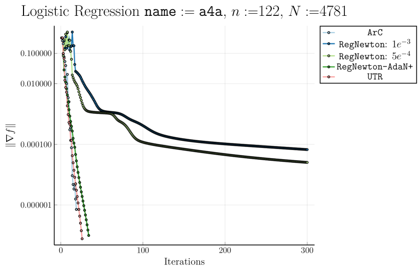
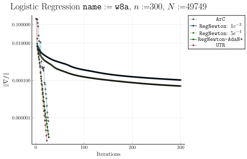
Refer to caption
Refer to caption
Figure 1: Logistic regression on LIBSVM instances: a4a (left) and w8a (right).

In FigureΒ 1, we profile the performance of these methods in minimizing the gradient norm. The results show that the adaptive universal trust-region method is comparable to ArC and RegNewton-AdaN+, implying its competence in minimizing the convex functions.

6 Conclusion

In this paper, we proposed a universal trust-region method that has a near-optimal rate of convergence under both convex and nonconvex settings. As a byproduct, we present an accelerated variant of the universal method with a complexity guarantee that naturally follows from the framework in [16]. To our knowledge, the complexity results for convex optimization are new for trust-region type methods. In that respect, our trust-region method is an ideal second-order method in terms of the desiderata in nonconvex and convex optimization with Lipschizian Hessians.

An adaptive universal method is presented for practice. As an example, we show when utilizing a specific adaptive rule with extra information on the eigenvalue of the Hessian matrices, the method converges to a second-order stationary point and has a local quadratic rate of convergence. We note it is entirely possible to use other update rules in AlgorithmΒ 3. In this direction, one may asymptotically decrease the regularization term $\sigma_{k}\to 0$ and even set it to zero if the iterate is sufficiently close to a local optimal, in which case, we preserve the global performance of the universal method. At the same time, at least obtain a local superlinear rate of convergence.

References

  • Nocedal and Wright [1999] Jorge Nocedal and StephenΒ J Wright. Numerical optimization. Springer, 1999.
  • Nesterov [2018] Yurii Nesterov. Lectures on convex optimization, volume 137. Springer, 2018.
  • Lan [2020] George Lan. First-order and Stochastic Optimization Methods for Machine Learning. Springer Series in the Data Sciences. Springer International Publishing, 2020.
  • Beck [2017] Amir Beck. First-order methods in optimization. SIAM, 2017.
  • Royer and Wright [2018] ClΓ©mentΒ W Royer and StephenΒ J Wright. Complexity analysis of second-order line-search algorithms for smooth nonconvex optimization. SIAM Journal on Optimization, 28(2):1448–1477, 2018.
  • Zhang etΒ al. [2022] Chuwen Zhang, Dongdong Ge, Chang He, BoΒ Jiang, Yuntian Jiang, Chenyu Xue, and Yinyu Ye. A homogenous second-order descent method for nonconvex optimization. arXiv preprint arXiv:2211.08212, 2022.
  • Curtis etΒ al. [2018] FrankΒ E Curtis, Zachary Lubberts, and DanielΒ P Robinson. Concise complexity analyses for trust region methods. Optimization Letters, 12:1713–1724, 2018.
  • Nesterov and Polyak [2006] Yurii Nesterov and BorisΒ T Polyak. Cubic regularization of newton method and its global performance. Mathematical Programming, 108(1):177–205, 2006.
  • Cartis etΒ al. [2011a] Coralia Cartis, NicholasΒ IM Gould, and PhilippeΒ L Toint. Adaptive cubic regularisation methods for unconstrained optimization. part i: motivation, convergence and numerical results. Mathematical Programming, 127(2):245–295, 2011a.
  • Cartis etΒ al. [2011b] Coralia Cartis, NicholasΒ IM Gould, and PhilippeΒ L Toint. Adaptive cubic regularisation methods for unconstrained optimization. part ii: worst-case function-and derivative-evaluation complexity. Mathematical programming, 130(2):295–319, 2011b.
  • Nesterov [2021] Yurii Nesterov. Superfast second-order methods for unconstrained convex optimization. Journal of Optimization Theory and Applications, 191:1–30, 2021.
  • Nesterov [2008] YuΒ Nesterov. Accelerating the cubic regularization of newton’s method on convex problems. Mathematical Programming, 112(1):159–181, 2008.
  • Doikov etΒ al. [2022] Nikita Doikov, Konstantin Mishchenko, and Yurii Nesterov. Super-universal regularized newton method. arXiv preprint arXiv:2208.05888, 2022.
  • Doikov and Nesterov [2023] Nikita Doikov and Yurii Nesterov. Gradient regularization of Newton method with Bregman distances. Mathematical Programming, 2023.
  • Mishchenko [2023] Konstantin Mishchenko. Regularized newton method with global $\mathcal{O}(1/k^{2})$ convergence. SIAM Journal on Optimization, 33(3):1440–1462, 2023.
  • Doikov and Nesterov [2020] Nikita Doikov and Yurii Nesterov. Contracting proximal methods for smooth convex optimization. SIAM Journal on Optimization, 30(4):3146–3169, 2020.
  • Gratton etΒ al. [2023] Serge Gratton, Sadok Jerad, and PhilippeΒ L Toint. Yet another fast variant of newton’s method for nonconvex optimization. arXiv preprint arXiv:2302.10065, 2023.
  • Mizuno etΒ al. [1993] Shinji Mizuno, MichaelΒ J. Todd, and Yinyu Ye. On adaptive-step primal-dual interior-point algorithms for linear programming. Mathematics of Operations research, 18(4):964–981, 1993. Publisher: INFORMS.
  • Hanzely etΒ al. [2022] SlavomΓ­r Hanzely, Dmitry Kamzolov, Dmitry Pasechnyuk, Alexander Gasnikov, Peter RichtΓ‘rik, and Martin TakΓ‘c. A damped newton method achieves global $\mathcal{O}(1/k^{2})$ and local quadratic convergence rate. Advances in Neural Information Processing Systems, 35:25320–25334, 2022.
  • Nesterov and Nemirovskii [1994] Yurii Nesterov and Arkadii Nemirovskii. Interior-point polynomial algorithms in convex programming. SIAM, 1994.
  • Conn etΒ al. [2000] AndrewΒ R Conn, NicholasΒ IM Gould, and PhilippeΒ L Toint. Trust region methods. SIAM, 2000.
  • Yuan [2000] Ya-xiang Yuan. A review of trust region algorithms for optimization. In Iciam, volumeΒ 99, pages 271–282, 2000.
  • Byrd etΒ al. [2006] RichardΒ H Byrd, Jorge Nocedal, and RichardΒ A Waltz. K nitro: An integrated package for nonlinear optimization. Large-scale nonlinear optimization, pages 35–59, 2006.
  • Curtis etΒ al. [2017] FrankΒ E Curtis, DanielΒ P Robinson, and Mohammadreza Samadi. A trust region algorithm with a worst-case iteration complexity of $\mathcal{O}(\epsilon^{-3/2})$ for nonconvex optimization. Mathematical Programming, 162:1–32, 2017.
  • Curtis etΒ al. [2021] FrankΒ E Curtis, DanielΒ P Robinson, ClΓ©mentΒ W Royer, and StephenΒ J Wright. Trust-region newton-cg with strong second-order complexity guarantees for nonconvex optimization. SIAM Journal on Optimization, 31(1):518–544, 2021.
  • Hamad and Hinder [2022] Fadi Hamad and Oliver Hinder. A consistently adaptive trust-region method. Advances in Neural Information Processing Systems, 35:6640–6653, 2022.
  • Luenberger and Ye [2021] DavidΒ G. Luenberger and Yinyu Ye. Linear and Nonlinear Programming, volume 228 of International Series in Operations Research & Management Science. Springer International Publishing, Cham, 2021.
  • Cartis etΒ al. [2022] Coralia Cartis, NicholasΒ IM Gould, and PhilippeΒ L Toint. Evaluation Complexity of Algorithms for Nonconvex Optimization: Theory, Computation and Perspectives. SIAM, 2022.
  • Curtis and Wang [2023] FrankΒ E. Curtis and QiΒ Wang. Worst-Case Complexity of TRACE with Inexact Subproblem Solutions for Nonconvex Smooth Optimization. SIAM Journal on Optimization, 33(3):2191–2221, 2023.
  • Lu etΒ al. [2018] Haihao Lu, RobertΒ M Freund, and Yurii Nesterov. Relatively smooth convex optimization by first-order methods, and applications. SIAM Journal on Optimization, 28(1):333–354, 2018.
  • He etΒ al. [2023] Chang He, Yuntian Jiang, Chuwen Zhang, Dongdong Ge, BoΒ Jiang, and Yinyu Ye. Homogeneous second-order descent framework: A fast alternative to newton-type methods. arXiv preprint arXiv:2306.17516, 2023.
  • Ye [1991] Yinyu Ye. A New Complexity Result on Minimization of a Quadratic Function with a Sphere Constraint. In Recent Advances in Global Optimization, volume 176, pages 19–31. Princeton University Press, 1991.
  • Ye [1994] Yinyu Ye. Combining Binary Search and Newton’s Method to Compute Real Roots for a Class of Real Functions. Journal of Complexity, 10(3):271–280, 1994.
  • Gould etΒ al. [2015] Nicholas I.Β M. Gould, Dominique Orban, and PhilippeΒ L. Toint. CUTEst: a Constrained and Unconstrained Testing Environment with safe threads for mathematical optimization. Computational Optimization and Applications, 60(3):545–557, 2015.
  • Dussault [2020] Jean-Pierre Dussault. A Unified Efficient Implementation of Trust-region Type Algorithms for Unconstrained Optimization. INFOR: Information Systems and Operational Research, 58(2):290–309, 2020.

Appendix

Appendix A Proof to RemarkΒ 3.1

Proof.

It suffices to show linear convergence in Line 6 of AlgorithmΒ 2 with respect to $\delta=O(\epsilon^{2/3})$. Then the total iteration complexity $\tilde{O}(\epsilon^{-1/3})$ follows from [16, Corollary 3.3]. Since $h_{k+1}(x)$ is uniformly convex of degree three, i.e., there exists $\sigma>0$ such that

$$h_{k+1}(y)\geq h_{k+1}(x)+\nabla h_{k+1}(x)^{T}(y-x)+\frac{\sigma}{3}\|y-x\|^{3},\quad\forall x,y\in\mathbb{R}^{n}$$ (A.1)

by the fact that $f(x)$ is convex and the Bregman distance $\beta_{d}(x;y)$ is uniformly convex. Assuming that $f$ is third-order differentiable, we can set the goal to minimize $h(x)$ (omitting the subscript for simplicity) by the universal trust-region method (AlgorithmΒ 1).

By (2.15) - (2.16), if the dual variable $\lambda_{k}=0$, we have

$$h(x_{k+1})\leq h(x_{k}),\quad\|\nabla h(x_{k+1})\|\leq\frac{1}{6}\|\nabla h(x_{k})\|;$$ (A.2)

otherwise, Ξ»kβ‰ 0subscriptπœ†π‘˜0\lambda_{k}\neq 0, we recall (3.7):

$$\|\nabla h(x_{k+1})\|\leq\frac{19}{18}\|\nabla h(x_{k})\|,$$

so we have:

$\displaystyle h(x_{k+1})-h(x_{k})$ $\displaystyle\leq-\frac{1}{81\sqrt{M}}\|\nabla h(x_{k})\|^{3/2}$ (A.3)
$\displaystyle=-\frac{1}{81\sqrt{M}}\cdot\frac{\|\nabla h(x_{k})\|^{2}}{\|\nabla h(x_{k})\|^{1/2}}$
$\displaystyle\leq-\frac{4}{361\sqrt{M}}\cdot\frac{\|\nabla h(x_{k+1})\|^{2}}{\|\nabla h(x_{k})\|^{1/2}}.$

In the sequel, the analysis is standard. We denote the $x_{j_{\delta}}$ as the first iterate such that $\|\nabla h(x_{j_{\delta}})\|\leq\delta$. Following the same nomenclature throughout this paper, we partition the set of iterates into β„±jΞ΄={k≀jδ∣λkβ‰ 0}subscriptβ„±subscript𝑗𝛿conditional-setπ‘˜subscript𝑗𝛿subscriptπœ†π‘˜0\mathcal{F}_{j_{\delta}}=\{k\leq j_{\delta}\mid\lambda_{k}\neq 0\} and $\mathcal{G}_{j_{\delta}}=\{k\leq j_{\delta}\mid\lambda_{k}=0\}$. By [14, Theorem 6], we obtain that

$$|\mathcal{F}_{j_{\delta}}|\leq O\left(\log\frac{\|\nabla h(x_{0})\|}{\delta}\right).$$

Therefore, using a similar argument in TheoremΒ 3.2, it follows

$$\left|\mathcal{F}_{j_{\delta}}\right|+\left|\mathcal{G}_{j_{\delta}}\right|\leq O\left(\log\frac{\|\nabla h(x_{0})\|}{\delta}\right),$$

which completes the proof. ∎

Appendix B Proof of LemmaΒ 4.1

Proof.

It is sufficient to show that for every $k$-th outer iteration, whenever the parameter $\rho_{k}^{(j)}$ satisfies

$$\rho_{k}^{(j)}\geq\max\left\{\sqrt{\frac{M}{12(1-32\eta)}},\sqrt{\frac{M}{6(1-8\eta)}},\sqrt{\frac{M}{32\xi-8}},\sqrt{\frac{M}{8\xi}}\right\},$$ (B.1)

the inner loop will terminate. Firstly, we consider the case where $\|g_{k}\|\leq\epsilon$ and $\lambda_{\min}(H_{k})\leq-\rho_{k}^{(j)}\epsilon^{1/2}$. To facilitate the analysis, we introduce the concept of an eigenpoint within the trust region, i.e.

$$d_{k}^{E}:=\frac{\epsilon^{1/2}}{2\rho_{k}^{(j)}}v_{k}\quad v_{k}^{T}g_{k}\leq 0,$$ (B.2)

where $v_{k}$ is the unit eigenvector corresponding to the smallest eigenvalue $\lambda_{\min}(H_{k})$. Note that for the eigenpoint $d_{k}^{E}$, it follows

$$g_{k}^{T}d_{k}^{E}+\frac{1}{2}\left(d_{k}^{E}\right)^{T}H_{k}d_{k}^{E}\leq\frac{1}{2}\left(d_{k}^{E}\right)^{T}H_{k}d_{k}^{E}\leq-\frac{1}{8\rho_{k}^{(j)}}\epsilon^{3/2},$$

and since the eigenpoint is feasible, once the parameter $\rho_{k}^{(j)}$ satisfies

ρk(j)β‰₯M6​(1βˆ’8​η),superscriptsubscriptπœŒπ‘˜π‘—π‘€618πœ‚\rho_{k}^{(j)}\geq\sqrt{\frac{M}{6(1-8\eta)}},

we have

$\displaystyle f(x_{k}+d_{k}^{(j)})-f(x_{k})$ $\displaystyle\leq g_{k}^{T}d_{k}^{(j)}+\frac{1}{2}\left(d_{k}^{(j)}\right)^{T}H_{k}d_{k}^{(j)}+\frac{M}{6}\left\|d_{k}^{(j)}\right\|^{3}$
$\displaystyle\leq g_{k}^{T}d_{k}^{E}+\frac{1}{2}\left(d_{k}^{E}\right)^{T}H_{k}d_{k}^{E}+\frac{M}{6}\left\|d_{k}^{(j)}\right\|^{3}$
$\displaystyle\leq-\frac{1}{8\rho_{k}^{(j)}}\epsilon^{3/2}+\frac{M}{48(\rho_{k}^{(j)})^{3}}\epsilon^{3/2}.$
$\displaystyle\leq-\frac{\eta}{\rho_{k}^{(j)}}\epsilon^{3/2},$ (B.3)

where the second inequality is from the optimality, the third inequality is because of (2.7b) and (2.7d). As a result, the sufficient descent is satisfied.

When $\|g_{k}\|>\epsilon$, we have three possible outcomes:

  • β€’

    The first case is

    $$\lambda_{\min}(H_{k})\leq-\rho_{k}^{(j)}\|g_{k}\|^{1/2}.$$

    The analysis is the same as in the above case, except that we need to replace $\epsilon$ with $\|g_{k}\|$.

  • β€’

    The second case is

    Ξ»min​(Hk)β‰₯ρk(j)​‖gkβ€–1/2,subscriptπœ†subscriptπ»π‘˜superscriptsubscriptπœŒπ‘˜π‘—superscriptnormsubscriptπ‘”π‘˜12\lambda_{\min}(H_{k})\geq\rho_{k}^{(j)}\|g_{k}\|^{1/2},

    and we need to divide this case into two subcases. The first one is that the dual variable $\lambda_{k}^{(j)}>0$, then it follows $\left\|d_{k}^{(j)}\right\|=\frac{1}{2\rho_{k}^{(j)}}\|g_{k}\|^{1/2}$, moreover, once the parameter $\rho_{k}^{(j)}$ satisfies

    ρk(j)β‰₯M6​(1βˆ’8​η),superscriptsubscriptπœŒπ‘˜π‘—π‘€618πœ‚\rho_{k}^{(j)}\geq\sqrt{\frac{M}{6(1-8\eta)}},

    we have

    $\displaystyle f(x_{k}+d_{k}^{(j)})-f(x_{k})$ $\displaystyle\leq g_{k}^{T}d_{k}^{(j)}+\frac{1}{2}(d_{k}^{(j)})^{T}H_{k}^{(j)}d_{k}^{(j)}+\frac{M}{6}\left\|d_{k}^{(j)}\right\|^{3}$
    $\displaystyle=-\frac{1}{2}(d_{k}^{(j)})^{T}H_{k}^{(j)}d_{k}^{(j)}-\lambda_{k}^{(j)}\left\|d_{k}^{(j)}\right\|^{2}+\frac{M}{6}\left\|d_{k}^{(j)}\right\|^{3}$
    $\displaystyle\leq-\frac{1}{2}\rho_{k}^{(j)}\|g_{k}\|^{1/2}\left\|d_{k}^{(j)}\right\|^{2}+\frac{M}{6}\left\|d_{k}^{(j)}\right\|^{3}$
    $\displaystyle\leq-\frac{\eta}{\rho_{k}^{(j)}}\|g_{k}\|^{3/2}.$ (B.4)

    On the other hand, if the dual variable $\lambda_{k}^{(j)}=0$, once the parameter $\rho_{k}^{(j)}$ satisfies

    $$\rho_{k}^{(j)}\geq\sqrt{\frac{M}{8\xi}},$$

    we have

    $\displaystyle\|\nabla f(x_{k}+d_{k}^{(j)})\|$ $\displaystyle\leq\|H_{k}^{(j)}d_{k}^{(j)}+g_{k}\|+\frac{M}{2}\left\|d_{k}^{(j)}\right\|^{2}$
    $\displaystyle=\frac{M}{2}\left\|d_{k}^{(j)}\right\|^{2}$ (B.5)
    $\displaystyle=\frac{M}{8\left(\rho_{k}^{(j)}\right)^{2}}\|g_{k}\|$ (B.6)
    $\displaystyle\leq\xi\|g_{k}\|.$ (B.7)

    It is easy to see the function value is decreasing.

  • β€’

    The third case is

    $$-\rho_{k}^{(j)}\|g_{k}\|^{1/2}<\lambda_{\min}(H_{k})<\rho_{k}^{(j)}\|g_{k}\|^{1/2},$$

    similarly, if $\lambda_{k}^{(j)}>0$, then $\left\|d_{k}^{(j)}\right\|=\frac{1}{4\rho_{k}^{(j)}}\|g_{k}\|^{1/2}$, once the parameter $\rho_{k}^{(j)}$ satisfies

    $$\rho_{k}^{(j)}\geq\sqrt{\frac{M}{12(1-32\eta)}},$$

    we have

    $\displaystyle f(x_{k}+d_{k}^{(j)})-f(x_{k})$ $\displaystyle\leq g_{k}^{T}d_{k}^{(j)}+\frac{1}{2}(d_{k}^{(j)})^{T}H_{k}^{(j)}d_{k}^{(j)}+\frac{M}{6}\left\|d_{k}^{(j)}\right\|^{3}$
    $\displaystyle=-\frac{1}{2}(d_{k}^{(j)})^{T}H_{k}^{(j)}d_{k}^{(j)}-\lambda_{k}^{(j)}\left\|d_{k}^{(j)}\right\|^{2}-\rho_{k}^{(j)}\|g_{k}\|^{1/2}\left\|d_{k}^{(j)}\right\|^{2}+\frac{M}{6}\left\|d_{k}^{(j)}\right\|^{3}$
    $\displaystyle\leq-\frac{1}{2}\rho_{k}^{((j)}\|g_{k}\|^{1/2}\left\|d_{k}^{(j)}\right\|^{2}+\frac{M}{6}\left\|d_{k}^{(j)}\right\|^{3}$
    $\displaystyle\leq-\frac{\eta}{\rho_{k}^{(j)}}\|g_{k}\|^{3/2}.$ (B.8)

    On the other hand, if $\lambda_{k}^{(j)}=0$, once the parameter $\rho_{k}^{(j)}$ satisfies

    $$\rho_{k}^{(j)}\geq\sqrt{\frac{M}{32\xi-8}},$$

    we have

    $\displaystyle\|\nabla f(x_{k}+d_{k}^{(j)})\|$ $\displaystyle\leq\|H_{k}^{(j)}d_{k}^{(j)}+g_{k}\|+\frac{M}{2}\left\|d_{k}^{(j)}\right\|^{2}$
    $\displaystyle=\rho_{k}^{(j)}\|g_{k}\|^{1/2}\left\|d_{k}^{(j)}\right\|+\frac{M}{2}\left\|d_{k}^{(j)}\right\|^{2}$
    $\displaystyle=\frac{1}{4}\|g_{k}\|+\frac{M}{32\left(\rho_{k}^{(j)}\right)^{2}}\|g_{k}\|$
    $\displaystyle\leq\xi\|g_{k}\|.$ (B.9)

    Also, from the last but one line of (B.8), we have $f(x_{k}+d_{k}^{(j)})-f\left(x_{k}\right)\leq 0$.

In summary, we show in all cases, the inner loop safely terminates as $\rho_{k}^{(j)}$ reaches a bounded constant. ∎