Towards a Post-Market Monitoring Framework for Machine Learning-based Medical Devices: A case study

Abstract

After a machine learning (ML)-based system is deployed in clinical practice, performance monitoring is important to ensure the safety and effectiveness of the algorithm over time. The goal of this work is to highlight the complexity of designing a monitoring strategy and the need for a systematic framework that compares the multitude of monitoring options. One of the main decisions is choosing between using real-world (observational) versus interventional data. Although the former is the most convenient source of monitoring data, it exhibits well-known biases, such as confounding, selection, and missingness. In fact, when the ML algorithm interacts with its environment, the algorithm itself may be a primary source of bias. On the other hand, a carefully designed interventional study that randomizes individuals can explicitly eliminate such biases, but the ethics, feasibility, and cost of such an approach must be carefully considered. Beyond the decision of the data source, monitoring strategies vary in the performance criteria they track, the interpretability of the test statistics, the strength of their assumptions, and their speed at detecting performance decay. As a first step towards developing a framework that compares the various monitoring options, we consider a case study of an ML-based risk prediction algorithm for postoperative nausea and vomiting (PONV). Bringing together tools from causal inference and statistical process control, we walk through the basic steps of defining candidate monitoring criteria, describing potential sources of bias and the causal model, and specifying and comparing candidate monitoring procedures. We hypothesize that these steps can be applied more generally, as causal inference can address other sources of biases as well.

1 Introduction

After a machine learning (ML)-based system is deployed in clinical practice, performance monitoring of the algorithm is necessary for mitigating risks (Breck et al., 2017; Finlayson et al., 2021; Feng et al., 2022b) and has been recognized by regulators as an essential aspect of good machine learning practice (GMLP) (U.S. Food and Drug Administration and Health Canada, 2021). Recent regulatory recommendations (US Food and Drug Administration, 2023b) have also highlighted how all medical devices—including ML-based algorithms—should institute quality systems (CFR Title 21 Part 820), which encompasses “monitor[ing] production processes to ensure that a device conforms to its specifications” (Subpart G). However, compared to the topic of model development and pre-market evaluation, the topic of post-deployment (i.e., post-market) performance monitoring has been relatively overlooked and more of an afterthought (Sculley et al., 2015; Paleyes et al., 2022; Zhang et al., 2022). This work aims to highlight the immense, underappreciated variety of monitoring options that address various statistical challenges in the post-market setting and the urgent need to develop a systematic framework to choose among these options.

On the surface, selecting a monitoring procedure appears simple: a natural choice is to monitor the same metrics used for initial model approval. This approach has been suggested in several works (Nishida and Yamauchi, 2007; Klaise et al., 2020; Schröder and Schulz, 2022; Corbin et al., 2023) and appears to satisfy recommendations from regulatory agencies (US Food and Drug Administration, 2023b). However, considering the many ways to measure performance, this is neither the only nor necessarily the best monitoring option. Procedures for monitoring different performance metrics vary in their trade-offs, so they should be tailored to suit specific situations. For instance, performance monitoring often places a strong emphasis on detecting performance decay as quickly as possible and, thus, the number of individuals exposed to a defective product (Montgomery, 2013). In this case, monitoring changes in a measure like AUC may be suboptimal because it is a relatively “coarse” metric (Pencina et al., 2008). Instead, as we highlight later, it may be more effective to monitor other measures that are less commonly assessed for initial approval but are much more sensitive.

Designing a post-market surveillance strategy encompasses not only the monitoring criteria but also what data to collect and what assumptions are required. For ML-based medical devices, the most convenient choice is observational data (e.g., electronic health records). Unfortunately, real-world data is well-known to contain many potential sources of biases (Pearl et al., 2016). Moreover, the ML algorithm itself may be a significant source of bias that changes the data generating process (Chaney et al., 2018; Perdomo et al., 2020). For instance, risk prediction models modify treatment patterns, and diagnostic models modify disease verification (Paxton et al., 2013; Lenert et al., 2019; Liley et al., 2021; Begg and Greenes, 1983; Pepe, 2003; US Food and Drug Administration, 2007). Most monitoring algorithms in the statistical process control (SPC) literature assume an ideal data setting and are not equipped to analyze real-world data (Montgomery, 2013; Qiu, 2013); if directly applied, they can have overly large false positive rates and/or significantly delayed time to detection. Recent works that address such biases vary in their monitoring criteria and the assumptions they need for identifiability. For example, monitoring the mean of a process using inverse weighting typically requires assuming a nonzero probability of treatment for each subgroup (positivity) and reliable estimation of the dynamic treatment patterns, on top of conditional exchangeability (Steiner and MacKay, 2001; Sun et al., 2014; Cook et al., 2015; FDA Sentinel program, 2014). In contrast, methods for monitoring algorithmic fairness and conditional performance measures can make weaker (or even no) assumptions regarding positivity but may be less interpretable (Feng et al., 2022a).

Rather than relying on observational data, one could consider generating interventional data, such as through randomization of treatment. This forcibly eliminates (some of the) major sources of bias so that the aforementioned identifiability assumptions are no longer needed. The challenge in gathering interventional data is determining the ethics and feasibility of such an approach. Nevertheless, intervention could be acceptable in certain scenarios, particularly if it drastically improves the long-term safety and effectiveness of the ML algorithm. Indeed, randomization is now being explored to monitor ML-based algorithms in healthcare (Horwitz et al., 2019; Harris et al., 2022) and detect changes in patient response to eHealth interventions (Mohr et al., 2013; Kumar et al., 2013).

Given the range of monitoring options, how does one choose between the many options for a given problem setting? Research originated or encouraged by regulatory bodies has been instrumental in developing roadmaps and reporting standards for evaluating medical products using real-world data (Cook et al., 2012; Petersen and van der Laan, 2014; Wu et al., 2023; Ho et al., 2023; Dang et al., 2023). These efforts have informed regulatory practices, guidelines for industry, and even approval of medical products (Desai et al., 2021; U.S. Food and Drug Administration and Health Canada, 2021; US Food and Drug Administration, 2021, 2023a). Nevertheless, existing frameworks are more in line with the problem of performance evaluation and not performance monitoring. There has been little discussion on how to assess and compare monitoring strategies for ML-based devices in the post-market setting. To this end, we take the first steps towards such a framework through a case study, where the goal is to design a monitoring strategy for a hypothetical ML-based risk prediction algorithm for Postoperative Nausea and Vomiting (PONV). Merging ideas from causal inference with SPC, we walk through four basic steps:

1. Define potential monitoring criteria

2. Enumerate sources of bias and define the causal model

3. Describe candidate monitoring strategies

4. Compare the pros and cons of candidate strategies

As the causal framework is well-equipped to analyze various sources of bias (e.g., missingness, selection bias, and confounding (Hernán et al., 2004; Hernán and Cole, 2009; Mohan and Pearl, 2021)), we hypothesize that these steps form a general roadmap for enumerating and assessing monitoring options. This case study also highlights the value of designing monitoring plans proactively: Prior to model deployment (i.e., during the algorithm development stage and initial assessment stages), we are limited by fewer constraints and can consider more options, which may ultimately lead to better design choices.

2 The case study: ML-based risk prediction algorithms

Our central case study is an algorithm for predicting a patient’s risk of developing PONV after surgery. Postoperative nausea and/or vomiting (PONV) is one of the most common side effects of anesthesia. Suppose the algorithm outputs for each patient an estimate of their risk of PONV if the antiemetic (i.e., antinausea) medications are or are not given. The clinician decides the treatment strategy based on the algorithm’s results. Suppose the initial algorithm was approved for clinical use based on its average negative predictive value (NPV) and positive predictive value (PPV). The ML algorithm is allowed to evolve based on prior observations, according to some predefined change control plan (US Food and Drug Administration, 2023b).

Notation. Let $X_{t}$ represent features for a patient drawn from the population at time $t$, uniformly at random. $A_{t}$ is a binary variable indicating whether the patient has or has not received antiemetic medications ($a_{t}=1$ versus $a_{t}=0$, respectively). Using potential outcomes notation, $Y_{t}(a_{t})$ is a binary outcome which indicates if the patient develops PONV under treatment $a_{t}$, where $Y_{t}(a_{t})=1$ means the patient does. For convenience, let $Y_{t}:=Y_{t}(A_{t})$ denote the observed outcome under the usual consistency assumption (Hernán and Robins, 2010). $\hat{f}_{t}(x,a)$ is the predicted risk from the ML algorithm at time $t$, given patient variables $x$ and treatment $a$. In addition, let $\hat{y}_{t}$ be the binarized version of $\hat{f}_{t}$, e.g. $\hat{y}_{t}(x,a)=\mathbbm{1}\{\hat{f}_{t}(x,a)>b\}$ for some threshold $b$. To formally describe how information accumulates over time, we define the process $\{(X_{t},A_{t},Y_{t}(0),Y_{t}(1),\hat{f}_{t}):t=1,2,\cdots\}$ as being adapted to the filtration $\{\mathcal{F}_{t}:t=1,2,\cdots\}$, where $\mathcal{F}_{t}$ is the sigma field generated by the collection of observations up to time $t$, i.e. $(\hat{f}_{t},Y_{t-1},A_{t-1},X_{t-1},\cdots,Y_{1},A_{1},X_{1})$.

2.1 Step 1: List potential monitoring criteria

The first step is to define a pool of candidate monitoring criteria. That is, what properties can we use to determine if an ML algorithm is performing up to specifications (also called “in-control” in the SPC literature)? Here, we take a frequentist view and formally express each monitoring criterion as a null hypothesis and each monitoring procedure as a sequential hypothesis test. An alarm is fired when the null hypothesis is rejected.

Below, we list three candidate criteria based on monitoring the PPV/NPV metrics, from the most interpretable and least strict to the least interpretable and most strict. Increasing stringency of the criteria also corresponds to increasing strength along the model calibration hierarchy (Van Calster et al., 2016) and in their algorithmic fairness requirements.

Criterion 1: The average PPV/NPVs should be maintained above some thresholds. For predefined thresholds $\{c_{a\upsilon}:a,\upsilon\in\{0,1\}\}$, this criterion corresponds to the null hypothesis

$$H_{0,C1}^{\operatorname{causal}} :\Pr\left(Y_{t}(a)=\upsilon|\hat{y}_{t}(X_{t},a)=\upsilon,\mathcal{F}_{t}\right)\geq c_{a\upsilon}\quad\forall t,a,\upsilon.$$ (1)

Note that by conditioning on $\mathcal{F}_{t}$ in (1), we condition on the ML algorithm $\hat{f}_{t}$. This avoids the situation where $\hat{f}_{t}$ is a random variable that needs to be marginalized over. The key benefit of this criterion is its interpretability, as it is a standard metric used in this case to approve the initial model.

Criterion 2: Subgroup-specific PPV/NPVs should be maintained above their respective thresholds. Motivated by concerns regarding algorithmic fairness, another criterion is that the PPV/NPV is maintained across predefined subgroups $\mathcal{S}_{1},\cdots,\mathcal{S}_{K}$, such as those defined by protected attributes. That is, for predefined subgroup-specific thresholds $\{c_{a\upsilon k}\}$, this criterion corresponds to checking the null hypothesis

$$H_{0,C2}^{\operatorname{causal}} :\Pr\left(Y_{t}(a)=\upsilon|\hat{y}_{t}(X_{t},a)=\upsilon,X_{t}\in\mathcal{S}_{k},\mathcal{F}_{t}\right)\geq c_{a\upsilon k}\quad\forall t,a,\upsilon,k.$$ (2)

This criterion is stricter than (1) and more sensitive to distribution shifts. However, to decide the thresholds $c_{a\upsilon k}$, we may need to collect more data to estimate the PPV/NPV per subgroup, which may delay the time to model deployment. Another concern is that any procedure that tests (2) must account for multiple testing, so it is unclear how powerful a monitoring procedure for (2) would ultimately be.

Criterion 3: The predicted probabilities should not be over-confident for any subgroup. Finally, an even stricter criterion than checking subgroup-specific PPV/NPVs is to check that the algorithm’s risk predictions are not overly extreme, in that the predicted risk should not be more extreme than the true adverse event rate for any subgroup for some tolerance $\delta\geq 0$. Formally, we check the null hypothesis:

$$H_{0,C3}^{\operatorname{causal}} :\hat{s}_{t}(x,a)\left(\hat{f}_{t}(x,a)-\Pr(Y_{t}(a)=1|x)\right)\leq\delta\quad\forall t,a,x,$$ (3)

where $\hat{s}_{t}(x,a)=\text{sign}\left(\hat{f}_{t}(x,a)-0.5\right)$ is the predicted class assuming a threshold of 0.5. This test can also be viewed as checking the strong calibration requirement, where the predicted probabilities are required to be within some distance of the true risk for each individual; models that satisfy the strong calibration requirement also satisfy strong notions of algorithmic fairness (Van Calster et al., 2016; Hebert-Johnson et al., 2018; Feng et al., 2023). It is the strictest criterion among the three and, thus, the most sensitive to dataset shifts. Although this can accelerate detection, the null hypothesis can be quite sensitive, particularly for small values of $\delta$, and may be violated only for a very small subgroup. Thus, we must be careful when interpreting a rejection of (3), as it could indicate a decay in model performance or that the model was not well-calibrated to begin with.

2.2 Step 2: List sources of bias across various data sources and define causal models.

To check the criteria from Section 2.1, we must consider what data sources may be used and the biases they exhibit. For this case study, suppose we can collect data from an observational setting where healthcare providers are free to decide how to use the ML algorithm or an interventional setting where patients are randomized to the two treatment options. Since PONV is not a life-threatening complication, hospitals may be willing to randomize, given the benefits in terms of model monitoring.

Definition in the interventional study	Definition in the observational study	Potential sources of bias
Study population: Which population is the ML algorithm intended for?
All surgical cases	Patients for which the algorithm was queried	Spectrum/referral bias: The ML algorithm is only queried for a subset of patients (Ladapo et al., 2013; US Food and Drug Administration, 2007), such as only the more difficult cases or subpopulations the algorithm is believed to perform well in.
Conditions of use: When is the ML algorithm queried for a risk prediction?
During the pre-operative phase	Variable timing, dependent on healthcare provider preferences	Off-label use: ML algorithm may be queried in settings that are not recommended, e.g. too early or late during a surgical case (Raji et al., 2022).
Benchmark/Outcomes: What is the reference or non-reference standard?
An expert panel is assembled to determine if a patient developed PONV.	Electronic phenotyping is used to determine if a patient developed PONV.	• Interfering medical interventions: Patients are treated with differing rates, driven in part by recommendations from the ML algorithm. • Differential measurement error: The electronic phenotyping algorithm has differential error rates (Wang et al., 2016; Sondhi et al., 2023). • Circular definitions: The outcome label is biased by the ML algorithm’s predictions, e.g. PONV is more likely to be documented for cases predicted to be at high risk (US Food and Drug Administration, 2007).

Table 1: Protocol components for monitoring an ML-based risk prediction algorithm for Postoperative Nausea and Vomiting (PONV)

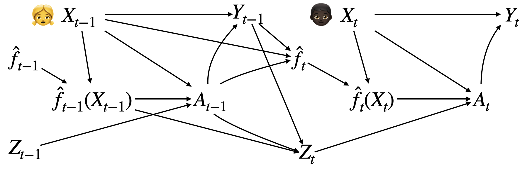
Figure 1: Causal model describing interfering medical interventions induced by an evolving ML-based risk prediction algorithm $\hat{f}_{t}$. $X_{t}$ denotes variables for the patient being queried for at time $t$. $Z_{t}$ denotes non-patient variables that may affect treatment decisions, such as past performance of the ML algorithm. $A_{t}$ denotes treatment assignment and $Y_{t}$ denotes the patient’s outcome. Note that $\hat{f}_{t}(X_{t})=(\hat{f}_{t}(X_{t},0),\hat{f}_{t}(X_{t},1))$.

We use the target trial emulation framework described in (Hernán and Robins, 2016) to compare the two data sources more formally. Recall that one view of causal inference is that it makes inferences from observational data about counterfactual quantities by emulating a target interventional study (Hernán, 2011). As such, we define the protocol components of the interventional and observational studies, as well as potential sources of bias that would lead to differences between the two studies. (For reference, protocol components are listed in (US Food and Drug Administration, 2013; De, 2023).) By organizing biases in this manner, we ensure no potential source of bias is missed. As seen in Table 1, the number of potential biases can be quite large. It may be helpful to prioritize which biases to focus on by identifying which ones are unlikely to occur or are less problematic. This often requires input from various stakeholders, including model developers, statistical experts, subject matter experts, and regulators.

For simplicity, among this list of potential biases, suppose we are mainly concerned with the problem of “interfering medical interventions” (IMI) (Paxton et al., 2013; Dyagilev and Saria, 2016; Lenert et al., 2019; Liley et al., 2021). (As we will see, things are complicated enough, even with just IMI!) IMI is the problem where the ML algorithm modifies treatment patterns, resulting in dependent “censoring” of counterfactual outcomes. In our case, the primary metric we want to monitor is NPV. If we estimated the NPV of $\hat{y}_{t}(\cdot,a)$ by directly calculating the NPV among patients who received treatment $a$, this estimate would be biased upwards because patients who are assigned treatment $a$ will tend to have lower risk if the algorithm is performing as expected. As illustrated in the simulation study in Section 2.4, this can lead to unnecessarily long detection delays.

To define the data-generating mechanism for the observational setting more formally, we assume data follows the directed acyclic graph (DAG) shown in Figure 1. IMI is caused by the arrows entering the treatment decision $A_{t}$. More specifically, we assume that $A_{t}$ depends on patient variables $X_{t}$, output from the ML algorithm $\hat{f}_{t}(X_{t},\cdot)$, and some other random variable $Z_{t}$, which represents non-patient factors that may influence a clinician’s decision to treat. For instance, $Z_{t}$ may be the performance of the ML algorithm recently.

2.3 Step 3: List the candidate monitoring strategies

We now describe various sequential procedures for detecting violations of the monitoring criteria listed in Step 1. Recall that sequential monitoring procedures are often defined by a chart statistic $\hat{C}(t)$ and some static or dynamic control limit $h(t)$ at each time $t$ (Zhang and Woodall, 2015). When the chart statistic exceeds the control limit, i.e., when $\hat{C}(t)>h(t)$, we fire an alarm. The control limit should be constructed to control behavior under the null, such as Type I error or average time to a false alarm (Chu et al., 1996; Zeileis, 2005; Qiu, 2013). It is often helpful to visualize this test via a control chart, which plots the two curves against each other (Figure 2).

This section presents variants of the CUSUM control chart (Page, 1954) for monitoring the aforementioned criteria given interventional versus observational data. The methods vary in what identifiability assumptions they require and how the chart statistics are defined. The Appendix describes a unified procedure for constructing control limits that control the Type I error.

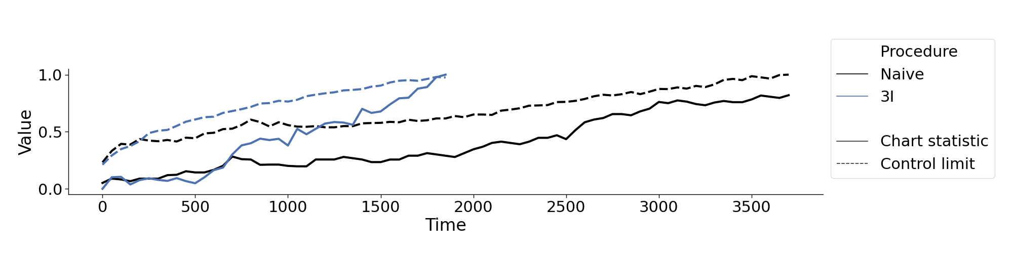
Figure 2: Example control charts, which plot the chart statistic (solid line) and control limit (dashed line) over time. An alarm is fired when the chart statistic exceeds the control limit.

2.3.1 Monitoring the average PPV/NPV (Criterion 1)

To motivate the chart statistic for monitoring (1), let us first suppose the counterfactual outcomes are observed. Over the time window from $t_{1}$ to $t_{2}$, the difference between the threshold and the true PPV/NPV can be estimated by

$$c_{a\upsilon}-\frac{\sum_{i=t_{1}}^{t_{2}}\mathbbm{1}\{Y_{i}(a)=\upsilon\}\mathbbm{1}\{\hat{y}_{i}(X_{i},a)=\upsilon\}}{\sum_{i=t_{1}}^{t_{2}}\mathbbm{1}\{\hat{y}_{i}(X_{i},a)=\upsilon\}}\quad\text{for }a,\upsilon=0,1.$$ (4)

Equivalently, we can rescale by the denominator and monitor $\Pr(Y_{i}(a)=\upsilon,\hat{y}_{i}(X_{i},a)=\upsilon|\mathcal{F}_{i})$ per

$$\frac{1}{t_{2}-t_{1}+1}\sum_{i=t_{1}}^{t_{2}}\left(c_{a\upsilon}-\mathbbm{1}\{Y_{i}(a)=\upsilon\}\right)\mathbbm{1}\{\hat{y}_{i}(X_{i},a)=\upsilon\}.$$ (5)

As the actual change time is unknown, we may define a scan statistic that calculates the maximum scaled differences starting from all possible changepoints. This gives us the CUSUM chart statistic

$$\hat{C}^{\operatorname{causal}}(t) =\max_{a,\tau,\upsilon}\sum_{i=\tau}^{t}(c_{a\upsilon}-\mathbbm{1}\{Y_{i}(a)=\upsilon\})\mathbbm{1}\{\hat{y}_{i}(X_{i},a)=\upsilon\}.$$ (6)

Option 1N: A naïve monitoring procedure

When we fail to consider the impact of IMI, one may choose to directly monitor the average PPV/NPV in the observed data using the chart statistic

$$\hat{C}^{1\texttt{N}}(t) =\max_{a,\tau,\upsilon}\sum_{i=\tau}^{t}(c_{a\upsilon}-\mathbbm{1}\{Y_{i}=\upsilon\})\mathbbm{1}\{\hat{y}_{i}(X_{i},A_{i})=\upsilon,A_{i}=a\}.$$ (7)

However, it is clear from the causal model that this quantity can be biased upwards or downwards depending on the treatment propensities. Thus, the alarm rate for such a procedure may be too high or too low.

Option 1I (Interventional)

To avoid biases introduced by IMI, one option is to randomize treatment with weights $p_{i}(a|x,z,\hat{f})\in(0,1)$. By design, we have that

$$\mathbbm{E}\left[\left(c_{a\upsilon}-\frac{\mathbbm{1}\{Y_{i}=\upsilon,A_{i}=a\}}{{p}_{i}(A_{i}|X_{i},Z_{i},\hat{f}_{i})}\right)\mathbbm{1}\left\{\hat{y}_{i}(X_{i},a)=\upsilon\right\}\right]=\mathbbm{E}\left[\left(c_{a\upsilon}-\mathbbm{1}\{Y_{i}(a)=\upsilon\}\right)\mathbbm{1}\left\{\hat{y}_{i}(X_{i},a)=\upsilon\right\}\right],$$ (8)

without needing to make any additional identifiability assumptions. Consequently, we can monitor the CUSUM chart statistic with inverse propensity weights

$$\hat{C}^{1\texttt{I}}(t) =\max_{\tau,a,\upsilon}\sum_{i=\tau}^{t}\left(c_{a\upsilon}-\frac{\mathbbm{1}\{Y_{i}=\upsilon,A_{i}=a\}}{p_{i}(A_{i}|X_{i},Z_{i},\hat{f}_{i})}\right)\mathbbm{1}\{\hat{y}_{i}(X_{i},a)=\upsilon\}.$$ (9)

Option 1O (Observational)

Let us continue with the above example, but we do not randomize treatment this time. Although (8) no longer holds in general, it does hold if we assume positivity—i.e. $p_{t}(A_{t}=1|X_{t},Z_{t},\hat{f}_{t})\in(0,1)$ almost everywhere for the oracle model $p_{t}$—and (sequential) conditional exchangeability—i.e. $Y_{t}(a)\perp A_{t}|X_{t},Z_{t},\mathcal{F}_{t}$—for all times $t$. Under these identifiability assumptions, we may extend (9) to the observational setting via a two-part solution similar to that in (Steiner and MacKay, 2001), where we (i) monitor PPV/NPVs assuming the propensity model is constant and (ii) monitor for changes in the propensity model. As the treatment propensities are unknown, we approximate (9) using estimates of the propensities instead. That is, letting $\hat{p}_{t}$ denote our estimate of the propensity model at time $t$, the chart statistic is defined as

$$\hat{C}^{1\texttt{O}}_{a}(t) =\max_{\tau,a,\upsilon}\sum_{i=\tau}^{t}\left(c_{a\upsilon}-\frac{\mathbbm{1}\{Y_{i}=\upsilon,A_{i}=a\}}{\hat{p}_{i}(A_{i}|X_{i},Z_{i},\hat{f}_{i})}\right)\mathbbm{1}\{\hat{y}_{i}(X_{i},a)=\upsilon\}.$$ (10)

Because (10) requires an estimate of the propensity model at $t=0$, this monitoring procedure requires conducting a “pre-monitoring study” after the deployment of the algorithm, where the sole purpose is to learn treatment assignment patterns (Feng et al., 2022a). During this phase, healthcare providers are asked to make treatment decisions based on predictions from the ML algorithm, but we only begin monitoring upon completion of this phase. (This pre-monitoring study is akin to Phase I SPC (Qiu, 2013).) Another drawback of this procedure is that we cannot verify the identifiability assumptions (Pearl et al., 2016). In fact, violations of the positivity condition are more likely to occur the more accurate the ML algorithm is (Lenert et al., 2019).

2.3.2 Monitoring subgroup-specific PPV/NPVs (Criterion 2)

We now extend the procedures from above to monitor subgroup-specific PPV/NPVs instead. For the interventional setting (Option 2I), we define the chart statistic as the maximum of (9) calculated for each subgroup, i.e.

$$\hat{C}^{2\texttt{I}}(t) =\max_{\tau,a,\upsilon,k}w_{k\upsilon}\sum_{i=\tau}^{t}\left(c_{a\upsilon k}-\frac{\mathbbm{1}\{Y_{i}=\upsilon,A_{i}=a\}}{p_{i}(A_{i}|X_{i},Z_{i},\hat{f}_{i})}\right)\mathbbm{1}\{\hat{y}_{i}(X_{i},a)=\upsilon,X_{i}\in\mathcal{S}_{k}\}.$$ (11)

where $w_{k\upsilon}$ is the weight associated with subgroup $\mathcal{S}_{k}$ and label $\upsilon$. For the observational setting (Option 2O), the chart statistic $\hat{C}^{2\texttt{O}}$ is exactly the same as $\hat{C}^{2\texttt{I}}$ except that the oracle propensity model is replaced by its estimate.

Compared to tests for Criterion 1, these tests are more powerful when performance decay is confined to only one of the subgroups. Also, in the observational setting, the major benefit of Option 2O over Option 1O is that the subgroup weights $w_{k\upsilon}$ can be selected to downweight subgroups with (near-)violations of the positivity condition; we can even remove such subgroups altogether. For instance, the empirical analyses in Section 2.4 set $w_{k\upsilon}$ to be the inverse of the estimated standard deviation of the summand in (11) for subgroup $\mathcal{S}_{k}$, with respect to the pre-change distribution. This way, the variance of the CUSUM statistic in each subgroup has roughly the same variance.

Potential concerns of these procedures are that: (i) their power depends on the overlap between $\{\mathcal{S}_{k}\}$ and the actual subgroup that experiences performance decay, (ii) more data needs to be collected upfront to estimate the initial PPV/NPV per subgroup and select the subgroup-specific thresholds $c_{ak}$, and (iii) we must perform multiplicity correction both across subgroups and over time to control the Type I error.

2.3.3 Checking for over-confident risk predictions (Criterion 3)

To test (3), we note that the expected residual

$$\mathbbm{E}\left[\hat{s}_{t}(X_{t},a)\left(\hat{f}_{t}(X_{t},a)-Y_{t}(a)\right)-\delta\mid X_{t}=x,\mathcal{F}_{t}\right]$$ (12)

is no larger than zero for almost every $x$ under the null. On the other hand, (12) will take on positive values at some values of $x$ under the alternative. So to check for violations of (3), one approach is to check if (12) when averaged over any marginal distribution of ${X}_{t}\mid\mathcal{F}_{t}$ is large. In particular, Option 3I monitors the following chart statistic in the interventional setting:

$$\hat{C}^{3\texttt{I}}(t) =\max_{\tau,k}w_{k\upsilon}\sum_{i=\tau}^{t}\left[\hat{s}_{t}(X_{t},a)\left(\hat{f}_{i}(X_{i},A_{i})-Y_{i}\right)-\delta\right]\mathbbm{1}\{X_{i}\in\mathcal{S}_{k}\}.$$ (13)

Compared to Options 1I and 2I, a major benefit of this approach is that there are no inverse weights, so it does not require the positivity assumption. However, the drawback is that (13) does not monitor a standard performance metric and is thus not very interpretable. Nevertheless, it may still be effective as a monitoring metric.

Another drawback of this approach is its sensitivity to miscalibration in the model, even in small subgroups. In addition, this procedure places more weight on checking predictions for treatments with higher propensities. So compared to the procedures with inverse weights, it will have lower power when distribution shifts concentrate in low-propensity regions.

In the observational setting, Option 3O assumes sequential conditional exchangeability so that (12) is equal to the observational quantity $\mathbbm{E}[\hat{s}_{t}(X_{t},A_{t})(Y_{t}-\hat{f}_{t}(X_{t},A_{t}))-\delta\mid A_{t}=a,X_{t}=x,\mathcal{F}_{t}]$ for almost every $(x,a)$. As such, chart statistic $\hat{C}^{3\texttt{O}}$ is defined exactly the same as $\hat{C}^{3\texttt{I}}$. Compared to Options 1O and 2O, the benefits of this approach are: (i) there is no need to model the propensity and the propensity model may even vary over time, (ii) we do not need to conduct a pre-monitoring study (as opposed to Option 2O), and (iii) the positivity assumption is not needed to control the Type I error.

2.4 Step 4: Compare candidate strategies

Finally, we are ready to compare candidate monitoring procedures. Table 2 summarizes the procedures in terms of their interpretability, fairness, data requirements, identifiability assumptions, and hyperparameters. In addition, we compare the statistical power of the different monitoring options using simulated data. As it is unlikely for a single monitoring procedure to perform the best across all simulation settings, the final decision should be based more heavily on the more likely scenarios.

Procedure	Interpretability	Fairness	Data requirements	Assumptions	Hyperparameters
1I	High	None	Interventional	Positivity	None
1O	High	None	Observational, Must conduct pre-monitoring phase	Positivity, Conditional Exchangeability	None
2I	High	Moderate	Interventional	Positivity	Subgroups, subgroup PPV/NPV
2O	High	Moderate	Observational, Must conduct pre-monitoring phase	Positivity, Conditional Exchangeability	Subgroups, subgroup PPV/NPV
3I	Medium	Strong	Interventional	None	Subgroups, tolerance level
3O	Medium	Strong	Observational, No pre-monitoring phase	Conditional Exchangeability	Subgroups, tolerance level

Table 2: Properties of different monitoring procedures

A comprehensive understanding of how the procedures compare requires performing a breadth of simulation studies. Settings to vary include randomization weights in the interventional setup, treatment propensities in the observational setup, the magnitude of the distribution shift, and the prevalence and time of performance decay. It can also be helpful to analyze the sensitivity of each procedure to violations of its assumptions. Given that we do not know how exactly the data will evolve over time, specifying realistic simulation settings will require input from stakeholders.

For this case study, suppose we believe healthcare providers will closely follow the ML algorithm’s recommendations in the observational setting. We compare against an interventional setting where randomization weights are defined using a logistic regression model that favors the recommended treatment but with less extreme propensities. An alternative view of this comparison is that it illustrates how different levels of clinician trust can impact detection delay. Here we conduct a limited simulation study to understand how the monitoring strategies from Section 2.3 compare. In practice, one would conduct a much more comprehensive simulation study to make a final decision.

We simulate a distribution shift at time $t=500$, during which the risk under treatment $a$ shifts in 40% of the population. We consider four simulation settings that vary the treatment ($a=0$ versus 1) and how much the risk increased (10% versus 20%). For all the monitoring criteria, the null hypotheses allow for only a 2% drop in the NPV or 2% difference in the true risk. As such, none of the null hypotheses are true. The control limit for each procedure controls the Type I error rate over 4000 time points at 10%. We implement procedures for Criteria 2 and 3 to monitor only two subgroups that partition the entire population, where the smaller subgroup corresponds to the one that experiences a performance decay in the future. Thus these results only reflect the situation where the subgroups are correctly specified; additional simulations are needed to assess operating characteristics when subgroups are misspecified. Full details of these simulations are provided in the Appendix.

As shown in Figure 3, there are substantial differences in power across the four simulation settings. Unsurprisingly, the naïve procedure performed poorly since its estimates are biased. Among the methods that correctly adjust for IMI, the most powerful approaches were those that monitor criterion 3. Monitoring criterion 2 was the second most powerful. Gaps in performance between criteria 2 and 3 methods were larger when the performance decay was smaller. Procedures for monitoring criterion 1 were the least powerful when the risk under treatment $a=1$ shifted, because the inverse propensity weights for estimating the average PPV/NPV were quite extreme.

Interestingly, collecting interventional data was beneficial only in certain circumstances. In particular, it led to faster detection when distribution shifted with respect to treatment $A=1$ but slower detection when the shift was with respect to treatment $A=0$. This is because the rate of assigning treatment $A=0$ was higher in the observational setting.

Based on Table 2 and results from this limited simulation study, Options 3I and 3O appear to be reasonable monitoring strategies. Option 3I is better for controlling the worst-case detection delay. However, if one believes that the worst-case scenario is unlikely to occur, then Option 3O will have comparable performance while being much more convenient. Regardless, going with either option implies that one needs to check that the ML algorithm is strongly calibrated prior to deployment and, if not, one should recalibrate the model.

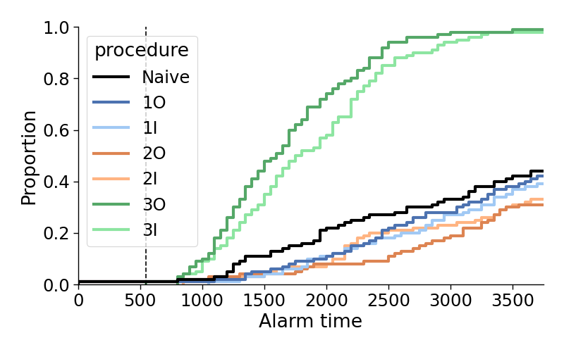
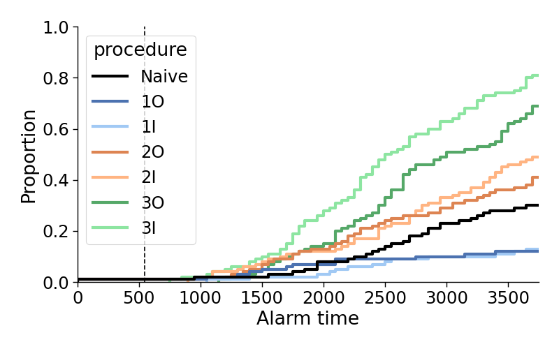
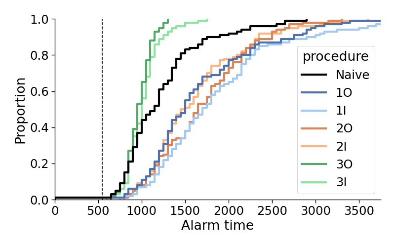
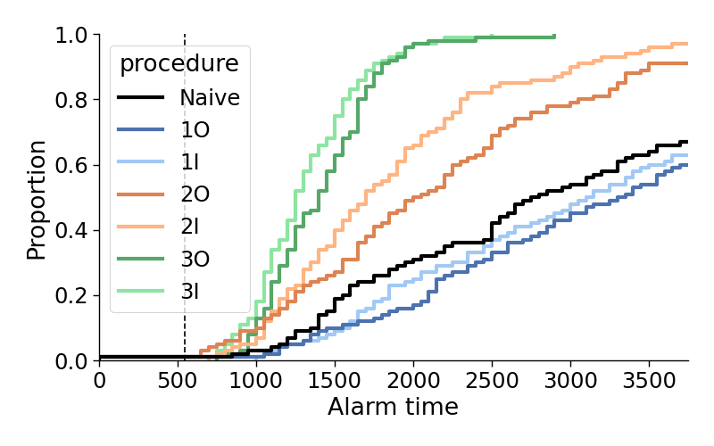
Figure 3: Comparison of monitoring procedures. Statistical power of different procedures, as characterized by the proportion of alarms fired at each time point. Dashed vertical line is the time of the distribution shift. Top and bottom rows simulate small and large shifts in the risk, respectively. Left and right columns simulate a shift in the risk under treatment $a=0$ and $a=1$, respectively.

3 Discussion

The aim of this work is to highlight the complexities behind designing a post-market surveillance strategy for ML-based medical devices. At a high level, this task can be summarized as choosing what data source to use and how to use it. To carry this out, one must choose between a multitude of options. Real-world data is plentiful but contains many sources of bias, while interventional data explicitly control for these biases but is much more limited in sample size. Given a data source, we must consider what monitoring criteria to use, which identifiability assumptions are needed (and reasonable), how to select hyperparameters, and more. Making these decisions requires input from diverse stakeholders, which is most effective when vendors are transparent regarding the data collection and analysis plan (US Food and Drug Administration, 2023a). Additional regulatory guidelines on the proper design of monitoring systems may also help steer these conversations. In this case study, we also uncover an important connection between algorithmic fairness and performance monitoring: checking for fairness violations can be a powerful approach to detecting model decay early.

In this workshop paper, we explored combining causal inference with statistical process control to help inform these decisions. Working through a general four-step framework, we enumerated and compared various approaches for monitoring a hypothetical ML-based risk prediction for PONV. Although we have only studied a single case study, we hypothesize that this framework is applicable more broadly and plan to demonstrate the generality of this framework in future work. Other directions for future research include delayed observation of the patient outcomes, how other types of monitoring data can be incorporated (e.g., that from instrumental variable designs), how we can augment observational data with interventional data, understanding interactions between multiple sources of bias, and monitoring the monitoring pipeline itself.

Appendix A Calculating control limits

For the procedures monitoring Criterion 3, we use the Monte Carlo procedure described in [Zhang and Woodall, 2015, Feng et al., 2023] to construct dynamic control limits (DCL). At each time $t$, we bootstrap $Y_{t}^{*}$ given $X_{t}$ under the worst-case null hypothesis satisfying (3), which corresponds to the case where $\Pr(Y_{t}^{*}=1|X_{t},\hat{f}_{t})=\hat{f}_{t}(X_{t},A_{t})+\delta$. For each of the bootstrap sequences, we calculate the corresponding chart statistics. The DCL is then chosen to satisfy an alpha spending function. Here, we use an alpha spending function that uniformly spends the $\alpha$ over time. This procedure provably controls the Type I error in finite samples [Feng et al., 2023].

In general, Criteria 1 and 2 are weaker than 3. To conduct a more fair comparison in the simulation studies, we construct DCLs for their corresponding test statistics to control the Type I error rate under Criteria 3. Thus the sensitivity of the methods for monitoring Criteria 1 or 2 are actually higher than they would be otherwise. Also, for illustrative purposes, we make the simplifying assumption in the simulation studies that the estimation error for the propensity model is negligible; this is true, for instance, if we had a sufficiently long pre-monitoring phase. To formally adjust for estimation error, one can use ideas such as that in [Gombay, 2002, Dette and Gösmann, 2020, Feng et al., 2022a].

Appendix B Simulation settings

There are two steps to conducting this simulation study. First, we must simulate a hypothetical ML algorithm for predicting a patient’s risk of developing PONV. Second, we simulate data to investigate the operating characteristics of various monitoring procedures. We discuss each step in turn.

Simulating the algorithm. We consider a setup with only two patient variables $X\in\mathbb{R}^{2}$, generated independently from a normal distribution with mean zero and variance 4. In the pre-deployment setting, we suppose the treatment was assigned uniformly at random. The data is generated from the logistic regression model

$$\text{logit}(y=1|x,a)=-0.5x_{1}-x_{2}+x_{1}a+2x_{2}a.$$

A random forest classifier is trained using 5000 observations, where $\hat{f}_{t}$ outputs the predicted risk (probability) of a patient developing PONV under a particular treatment.

Monitoring setup. In settings with no performance drift, we expect the ML algorithm to stay relatively stable over time. So in this limited simulation study, we do not update the ML algorithm over time. We suppose that treatment decisions are assigned according to a logistic regression model of the form

$$\text{logit}(a=1|x,\hat{f}_{t})=\beta\left[\hat{f}_{t}(x,a=1)-\hat{f}_{t}(x,a=0))\right]$$

for some $\beta\in\mathbb{R}$. We suppose $\beta=-6$ in the observational setting (i.e. clinicians closely follow recommendations from the ML algorithm) and $\beta=-2$ in the interventional setting (i.e. randomization weights favor following the ML algorithm). We simulate an increase of the risk in the subgroup where $x_{1}\in(-1,2)$ and $|x_{2}|<2.5$ under treatment $a$; this was chosen to reflect the more clinically interesting scenario where treatment decisions would change due to the distribution shift. The simulations vary in the magnitude of the increase (10% versus 20%) and the treatment for which risk increased ($a=0$ versus $a=1$). For computational speed, observations were monitored in batches of 50.

References

- Begg and Greenes [1983] Colin B Begg and Robert A Greenes. Assessment of diagnostic tests when disease verification is subject to selection bias. Biometrics, 39(1):207–215, 1983. URL http://www.jstor.org/stable/2530820.
- Breck et al. [2017] Eric Breck, Shanqing Cai, Eric Nielsen, Michael Salib, and D Sculley. The ML test score: A rubric for ML production readiness and technical debt reduction. In 2017 IEEE International Conference on Big Data (Big Data), pages 1123–1132. ieeexplore.ieee.org, December 2017. URL http://dx.doi.org/10.1109/BigData.2017.8258038.
- Chaney et al. [2018] Allison J B Chaney, Brandon M Stewart, and Barbara E Engelhardt. How algorithmic confounding in recommendation systems increases homogeneity and decreases utility. In Proceedings of the 12th ACM Conference on Recommender Systems, RecSys ’18, pages 224–232, New York, NY, USA, September 2018. Association for Computing Machinery. URL https://doi.org/10.1145/3240323.3240370.
- Chu et al. [1996] Chia-Shang James Chu, Maxwell Stinchcombe, and Halbert White. Monitoring structural change. Econometrica, 64(5):1045–1065, 1996. URL http://www.jstor.org/stable/2171955.
- Cook et al. [2012] Andrea J Cook, Ram C Tiwari, Robert D Wellman, Susan R Heckbert, Lingling Li, Patrick Heagerty, Tracey Marsh, and Jennifer C Nelson. Statistical approaches to group sequential monitoring of postmarket safety surveillance data: current state of the art for use in the Mini-Sentinel pilot. Pharmacoepidemiol. Drug Saf., 21 Suppl 1:72–81, January 2012. URL http://dx.doi.org/10.1002/pds.2320.
- Cook et al. [2015] Andrea J Cook, Robert D Wellman, Jennifer C Nelson, Lisa A Jackson, and Ram C Tiwari. Group sequential method for observational data by using generalized estimating equations: application to vaccine safety datalink. J. R. Stat. Soc. Ser. C Appl. Stat., 64(2):319–338, 2015. URL http://www.jstor.org/stable/24771896.
- Corbin et al. [2023] Conor K Corbin, Rob Maclay, Aakash Acharya, Sreedevi Mony, Soumya Punnathanam, Rahul Thapa, Nikesh Kotecha, Nigam H Shah, and Jonathan H Chen. DEPLOYR: a technical framework for deploying custom real-time machine learning models into the electronic medical record. J. Am. Med. Inform. Assoc., 30(9):1532–1542, August 2023. URL http://dx.doi.org/10.1093/jamia/ocad114.
- Dang et al. [2023] Lauren E Dang, Susan Gruber, Hana Lee, Issa Dahabreh, Elizabeth A Stuart, Brian D Williamson, Richard Wyss, Iván Díaz, Debashis Ghosh, Emre Kıcıman, Demissie Alemayehu, Katherine L Hoffman, Carla Y Vossen, Raymond A Huml, Henrik Ravn, Kajsa Kvist, Richard Pratley, Mei-Chiung Shih, Gene Pennello, David Martin, Salina P Waddy, Charles E Barr, Mouna Akacha, John B Buse, Mark van der Laan, and Maya Petersen. A causal roadmap for generating High-Quality Real-World evidence. May 2023. URL http://arxiv.org/abs/2305.06850.
- De [2023] Arkendra De. Statistical considerations and challenges for pivotal clinical studies of artificial intelligence medical tests for widespread use: Opportunities for Inter-Disciplinary collaboration. Stat. Biopharm. Res., 15(3):476–490, July 2023. URL https://doi.org/10.1080/19466315.2023.2169752.
- Desai et al. [2021] Rishi J Desai, Michael E Matheny, Kevin Johnson, Keith Marsolo, Lesley H Curtis, Jennifer C Nelson, Patrick J Heagerty, Judith Maro, Jeffery Brown, Sengwee Toh, Michael Nguyen, Robert Ball, Gerald Dal Pan, Shirley V Wang, Joshua J Gagne, and Sebastian Schneeweiss. Broadening the reach of the FDA sentinel system: A roadmap for integrating electronic health record data in a causal analysis framework. NPJ Digit Med, 4(1):170, December 2021. URL http://dx.doi.org/10.1038/s41746-021-00542-0.
- Dette and Gösmann [2020] Holger Dette and Josua Gösmann. A likelihood ratio approach to sequential change point detection for a general class of parameters. J. Am. Stat. Assoc., 115(531):1361–1377, July 2020. URL https://doi.org/10.1080/01621459.2019.1630562.
- Dyagilev and Saria [2016] Kirill Dyagilev and Suchi Saria. Learning (predictive) risk scores in the presence of censoring due to interventions. Mach. Learn., 102(3):323–348, March 2016. URL https://doi.org/10.1007/s10994-015-5527-7.
- FDA Sentinel program [2014] FDA Sentinel program. Creation of analytic dataset and conducting analysis for the group sequential inverse probability of treatment weighted (GS IPTW) regression tool. 2014. URL https://www.sentinelinitiative.org/sites/default/files/Methods/Mini-Sentinel_PROMPT_Group-Sequential-Inverse-Probability-of-Treatment-Weighted-Regression-Tool_Users-Guide_1.pdf.
- Feng et al. [2022a] Jean Feng, Alexej Gossmann, Gene Pennello, Nicholas Petrick, Berkman Sahiner, and Romain Pirracchio. Monitoring machine learning (ML)-based risk prediction algorithms in the presence of confounding medical interventions. November 2022a. URL http://arxiv.org/abs/2211.09781.
- Feng et al. [2022b] Jean Feng, Rachael V Phillips, Ivana Malenica, Andrew Bishara, Alan E Hubbard, Leo A Celi, and Romain Pirracchio. Clinical artificial intelligence quality improvement: towards continual monitoring and updating of AI algorithms in healthcare. npj Digital Medicine, 5(1):1–9, May 2022b. URL https://www.nature.com/articles/s41746-022-00611-y.
- Feng et al. [2023] Jean Feng, Alexej Gossmann, Romain Pirracchio, Nicholas Petrick, Gene Pennello, and Berkman Sahiner. Is this model reliable for everyone? testing for strong calibration. July 2023. URL http://arxiv.org/abs/2307.15247.
- Finlayson et al. [2021] Samuel G Finlayson, Adarsh Subbaswamy, Karandeep Singh, John Bowers, Annabel Kupke, Jonathan Zittrain, Isaac S Kohane, and Suchi Saria. The clinician and dataset shift in artificial intelligence. N. Engl. J. Med., 385(3):283–286, July 2021. URL http://dx.doi.org/10.1056/NEJMc2104626.
- Gombay [2002] Gombay. Parametric sequential tests in the presence of nuisance parameters. Theory Stoch. Process., 2002. URL https://www.researchgate.net/profile/Edit-Gombay/publication/228881435_Parametric_sequential_tests_in_the_presence_of_nuisance_parameters/links/0912f51193d6682ce5000000/Parametric-sequential-tests-in-the-presence-of-nuisance-parameters.pdf.
- Harris et al. [2022] Steve Harris, Tim Bonnici, Thomas Keen, Watjana Lilaonitkul, Mark J White, and Nel Swanepoel. Clinical deployment environments: Five pillars of translational machine learning for health. Frontiers in Digital Health, 4, 2022. URL https://www.frontiersin.org/articles/10.3389/fdgth.2022.939292.
- Hebert-Johnson et al. [2018] Ursula Hebert-Johnson, Michael Kim, Omer Reingold, and Guy Rothblum. Multicalibration: Calibration for the (Computationally-Identifiable) masses. International Conference on Machine Learning, 80:1939–1948, 2018. URL https://proceedings.mlr.press/v80/hebert-johnson18a.html.
- Hernán [2011] Miguel A Hernán. With great data comes great responsibility: publishing comparative effectiveness research in epidemiology. Epidemiology, 22(3):290–291, May 2011. URL http://dx.doi.org/10.1097/EDE.0b013e3182114039.
- Hernán and Cole [2009] Miguel A Hernán and Stephen R Cole. Invited commentary: Causal diagrams and measurement bias. Am. J. Epidemiol., 170(8):959–62; discussion 963–4, October 2009. URL http://dx.doi.org/10.1093/aje/kwp293.
- Hernán and Robins [2010] Miguel A Hernán and James M Robins. Causal inference, 2010.
- Hernán and Robins [2016] Miguel A Hernán and James M Robins. Using big data to emulate a target trial when a randomized trial is not available. Am. J. Epidemiol., 183(8):758–764, April 2016. URL http://dx.doi.org/10.1093/aje/kwv254.
- Hernán et al. [2004] Miguel A Hernán, Sonia Hernández-Díaz, and James M Robins. A structural approach to selection bias. Epidemiology, 15(5):615–625, September 2004. URL http://dx.doi.org/10.1097/01.ede.0000135174.63482.43.
- Ho et al. [2023] Martin Ho, Susan Gruber, Yixin Fang, Douglas E Faris, Pallavi Mishra-Kalyani, David Benkeser, and Mark van der Laan. Examples of applying RWE Causal-Inference roadmap to clinical studies. Stat. Biopharm. Res., pages 1–14, February 2023. URL https://doi.org/10.1080/19466315.2023.2177333.
- Horwitz et al. [2019] Leora I Horwitz, Masha Kuznetsova, and Simon A Jones. Creating a learning health system through Rapid-Cycle, randomized testing. N. Engl. J. Med., 381(12):1175–1179, September 2019. URL http://dx.doi.org/10.1056/NEJMsb1900856.
- Klaise et al. [2020] Janis Klaise, Arnaud Van Looveren, Clive Cox, Giovanni Vacanti, and Alexandru Coca. Monitoring and explainability of models in production. In Workshop on Challenges in Deploying and Monitoring Machine Learning Systems, July 2020. URL http://arxiv.org/abs/2007.06299.
- Kumar et al. [2013] Santosh Kumar, Wendy J Nilsen, Amy Abernethy, Audie Atienza, Kevin Patrick, Misha Pavel, William T Riley, Albert Shar, Bonnie Spring, Donna Spruijt-Metz, Donald Hedeker, Vasant Honavar, Richard Kravitz, R Craig Lefebvre, David C Mohr, Susan A Murphy, Charlene Quinn, Vladimir Shusterman, and Dallas Swendeman. Mobile health technology evaluation: the mhealth evidence workshop. Am. J. Prev. Med., 45(2):228–236, August 2013. URL http://dx.doi.org/10.1016/j.amepre.2013.03.017.
- Ladapo et al. [2013] Joseph A Ladapo, Saul Blecker, Michael R Elashoff, Jerome J Federspiel, Dorice L Vieira, Gaurav Sharma, Mark Monane, Steven Rosenberg, Charles E Phelps, and Pamela S Douglas. Clinical implications of referral bias in the diagnostic performance of exercise testing for coronary artery disease. J. Am. Heart Assoc., 2(6):e000505, December 2013. URL http://dx.doi.org/10.1161/JAHA.113.000505.
- Lenert et al. [2019] Matthew C Lenert, Michael E Matheny, and Colin G Walsh. Prognostic models will be victims of their own success, unless…. J. Am. Med. Inform. Assoc., 26(12):1645–1650, December 2019. URL http://dx.doi.org/10.1093/jamia/ocz145.
- Liley et al. [2021] James Liley, Samuel Emerson, Bilal Mateen, Catalina Vallejos, Louis Aslett, and Sebastian Vollmer. Model updating after interventions paradoxically introduces bias. International Conference on Artificial Intelligence and Statistics, 130:3916–3924, 2021. URL http://proceedings.mlr.press/v130/liley21a.html.
- Mohan and Pearl [2021] Karthika Mohan and Judea Pearl. Graphical models for processing missing data. J. Am. Stat. Assoc., 116(534):1023–1037, April 2021. URL https://doi.org/10.1080/01621459.2021.1874961.
- Mohr et al. [2013] David C Mohr, Ken Cheung, Stephen M Schueller, C Hendricks Brown, and Naihua Duan. Continuous evaluation of evolving behavioral intervention technologies. Am. J. Prev. Med., 45(4):517–523, October 2013.
- Montgomery [2013] Douglas C Montgomery. Statistical quality control. John Wiley & Sons, Nashville, TN, 7 edition, 2013.
- Nishida and Yamauchi [2007] Kyosuke Nishida and Koichiro Yamauchi. Detecting concept drift using statistical testing. In Discovery Science, pages 264–269. Springer Berlin Heidelberg, 2007. URL http://dx.doi.org/10.1007/978-3-540-75488-6_27.
- Page [1954] E S Page. Continuous inspection schemes. Biometrika, 41(1/2):100–115, 1954. URL http://www.jstor.org/stable/2333009.
- Paleyes et al. [2022] Andrei Paleyes, Raoul-Gabriel Urma, and Neil D Lawrence. Challenges in deploying machine learning: A survey of case studies. ACM Comput. Surv., 55(6):1–29, December 2022. URL https://doi.org/10.1145/3533378.
- Paxton et al. [2013] Chris Paxton, Alexandru Niculescu-Mizil, and Suchi Saria. Developing predictive models using electronic medical records: challenges and pitfalls. AMIA Annu. Symp. Proc., 2013:1109–1115, November 2013. URL https://www.ncbi.nlm.nih.gov/pubmed/24551396.
- Pearl et al. [2016] Judea Pearl, Madelyn Glymour, and Nicholas P Jewell. Causal Inference in Statistics: A Primer. John Wiley & Sons, January 2016. URL https://play.google.com/store/books/details?id=I0V2CwAAQBAJ.
- Pencina et al. [2008] Michael J Pencina, Ralph B D’Agostino, Sr, Ralph B D’Agostino, Jr, and Ramachandran S Vasan. Evaluating the added predictive ability of a new marker: from area under the ROC curve to reclassification and beyond. Stat. Med., 27(2):157–72; discussion 207–12, January 2008. URL http://dx.doi.org/10.1002/sim.2929.
- Pepe [2003] Margaret Sullivan Pepe. The Statistical Evaluation of Medical Tests for Classification and Prediction. Oxford University Press, 2003. URL https://market.android.com/details?id=book-UHQoAgAAQBAJ.
- Perdomo et al. [2020] Juan Perdomo, Tijana Zrnic, Celestine Mendler-Dünner, and Moritz Hardt. Performative prediction. In Hal Daumé Iii and Aarti Singh, editors, Proceedings of the 37th International Conference on Machine Learning, volume 119 of Proceedings of Machine Learning Research, pages 7599–7609. PMLR, 2020. URL https://proceedings.mlr.press/v119/perdomo20a.html.
- Petersen and van der Laan [2014] Maya L Petersen and Mark J van der Laan. Causal models and learning from data: integrating causal modeling and statistical estimation. Epidemiology, 25(3):418–426, May 2014. URL http://dx.doi.org/10.1097/EDE.0000000000000078.
- Qiu [2013] Peihua Qiu. Introduction to Statistical Process Control. Chapman and Hall/CRC, 1st edition edition, October 2013. URL https://www.taylorfrancis.com/books/mono/10.1201/b15016/introduction-statistical-process-control-peihua-qiu.
- Raji et al. [2022] Inioluwa Deborah Raji, I Elizabeth Kumar, Aaron Horowitz, and Andrew Selbst. The fallacy of AI functionality. In Proceedings of the 2022 ACM Conference on Fairness, Accountability, and Transparency, FAccT ’22, pages 959–972, New York, NY, USA, June 2022. Association for Computing Machinery. URL https://doi.org/10.1145/3531146.3533158.
- Schröder and Schulz [2022] Tim Schröder and Michael Schulz. Monitoring machine learning models: a categorization of challenges and methods. Data Science and Management, 5(3):105–116, September 2022. URL https://www.sciencedirect.com/science/article/pii/S2666764922000303.
- Sculley et al. [2015] D Sculley, Gary Holt, Daniel Golovin, Eugene Davydov, Todd Phillips, Dietmar Ebner, Vinay Chaudhary, Michael Young, Jean-François Crespo, and Dan Dennison. Hidden technical debt in machine learning systems. In C Cortes, N Lawrence, D Lee, M Sugiyama, and R Garnett, editors, Advances in Neural Information Processing Systems, volume 28. Curran Associates, Inc., 2015. URL https://proceedings.neurips.cc/paper/2015/file/86df7dcfd896fcaf2674f757a2463eba-Paper.pdf.
- Sondhi et al. [2023] Arjun Sondhi, Alexander S Rich, Siruo Wang, and Jeffery T Leek. Postprediction inference for clinical characteristics extracted with machine learning on electronic health records. JCO Clin Cancer Inform, 7:e2200174, May 2023. URL http://dx.doi.org/10.1200/CCI.22.00174.
- Steiner and MacKay [2001] Stefan H Steiner and R Jock MacKay. Monitoring processes with data censored owing to competing risks by using exponentially weighted moving average control charts. J. R. Stat. Soc. Ser. C Appl. Stat., 50(3):293–302, September 2001. URL https://academic.oup.com/jrsssc/article-pdf/50/3/293/48750653/jrsssc_50_3_293.pdf.
- Sun et al. [2014] Rena Jie Sun, John D Kalbfleisch, and Douglas E Schaubel. A weighted cumulative sum (WCUSUM) to monitor medical outcomes with dependent censoring. Stat. Med., 33(18):3114–3129, August 2014. URL http://dx.doi.org/10.1002/sim.6139.
- US Food and Drug Administration [2007] US Food and Drug Administration. Statistical guidance on reporting results from studies evaluating diagnostic tests. 2007. URL https://www.fda.gov/files/medical%20devices/published/Guidance-for-Industry-and-FDA-Staff---Statistical-Guidance-on-Reporting-Results-from-Studies-Evaluating-Diagnostic-Tests-%28PDF-Version%29.pdf.
- US Food and Drug Administration [2013] US Food and Drug Administration. Design considerations for pivotal clinical investigations for medical devices. Technical report, 2013. URL https://www.fda.gov/media/87363/download.
- US Food and Drug Administration [2021] US Food and Drug Administration. Examples of Real-World evidence (RWE) used in medical device regulatory decisions. Technical report, 2021. URL https://www.fda.gov/media/146258/download.
- US Food and Drug Administration [2023a] US Food and Drug Administration. Considerations for the use of Real-World data and Real-World evidence to support regulatory Decision-Making for drug and biological products. Technical report, August 2023a. URL https://www.fda.gov/regulatory-information/search-fda-guidance-documents/considerations-use-real-world-data-and-real-world-evidence-support-regulatory-decision-making-drug.
- US Food and Drug Administration [2023b] US Food and Drug Administration. Marketing submission recommendations for a predetermined change control plan for artificial Intelligence/Machine learning (AI/ML)-Enabled device software functions. Technical report, 2023b. URL https://www.fda.gov/media/166704/download.
- U.S. Food and Drug Administration and Health Canada [2021] U.S. Food and Drug Administration and Health Canada. Good machine learning practice for medical device development, October 2021. URL https://www.fda.gov/medical-devices/software-medical-device-samd/good-machine-learning-practice-medical-device-development-guiding-principles.
- Van Calster et al. [2016] Ben Van Calster, Daan Nieboer, Yvonne Vergouwe, Bavo De Cock, Michael J Pencina, and Ewout W Steyerberg. A calibration hierarchy for risk models was defined: from utopia to empirical data. J. Clin. Epidemiol., 74:167–176, June 2016. URL http://dx.doi.org/10.1016/j.jclinepi.2015.12.005.
- Wang et al. [2016] L E Wang, Pamela A Shaw, Hansie M Mathelier, Stephen E Kimmel, and Benjamin French. Evaluating risk-prediction models using data from electronic health records. Ann. Appl. Stat., 10(1):286–304, March 2016. URL http://dx.doi.org/10.1214/15-AOAS891.
- Wu et al. [2023] Ying Wu, Hongwei Wang, Jie Chen, and Hana Lee. Estimand in Real-World evidence study: From frameworks to application. In Weili He, Yixin Fang, and Hongwei Wang, editors, Real-World Evidence in Medical Product Development, pages 145–165. Springer International Publishing, Cham, 2023. URL https://doi.org/10.1007/978-3-031-26328-6_9.
- Zeileis [2005] Achim Zeileis. A unified approach to structural change tests based on ML scores, F statistics, and OLS residuals. Economet. Rev., 24(4):445–466, October 2005. URL https://doi.org/10.1080/07474930500406053.
- Zhang et al. [2022] Jie M Zhang, Mark Harman, Lei Ma, and Yang Liu. Machine learning testing: Survey, landscapes and horizons. IEEE Trans. Software Eng., 48(1):1–36, January 2022. URL http://dx.doi.org/10.1109/TSE.2019.2962027.
- Zhang and Woodall [2015] Xiang Zhang and William H Woodall. Dynamic probability control limits for risk-adjusted bernoulli CUSUM charts. Stat. Med., 34(25):3336–3348, November 2015. URL http://dx.doi.org/10.1002/sim.6547.