Classical Stability Margins by PID Control

Abstract

Proportional-Integral-Derivative (PID) control has been the workhorse of control technology for about a century. Yet to this day, designing and tuning PID controllers relies mostly on either tabulated rules (Ziegler-Nichols) or on classical graphical techniques (Bode). Our goal in this paper is to take a fresh look on PID control in the context of optimizing stability margins for low-order (first- and second-order) linear time-invariant systems. Specifically, we seek to derive explicit expressions for gain and phase margins that are achievable using PID control, and thereby gain insights on the role of unstable poles and nonminimum-phase zeros in attaining robust stability. In particular, stability margins attained by PID control for minimum-phase systems match those obtained by more general control, while for nonminimum-phase systems, PID control achieves margins that are no worse than those of general control modulo a predetermined factor. Furthermore, integral action does not contribute to robust stabilization beyond what can be achieved by PD control alone.

I Introduction

The primary goal of feedback regulation is to maintain stability and performance in the presence of modeling uncertainty and external disturbances. Amongst the metrics that are commonly used to quantify robustness against such factors, traditionally, the most important have been gain and phase margins, various types of induced norms ($H_{\infty}$, $L_{\infty}$), the gap metric, the structured singular value, and so forth. Each of these, and a few others, have been the subject of respective chapters in the modern robust control literature. Herein, we focus on gain and phase margins that historically have been the first to be considered. Interestingly but perhaps unsurprisingly, these same metrics have also been the first to be tackled in the waning years of the 1970’s with the modern tools of analytic function theory that gave rise to optimal designs [1, 2, 3]; see also [4, 5, 6] as well as [7, Chapter 11].

Gain and phase margins quantify tolerance of stability of a feedback system to perturbation in the respective features of its transfer function, i.e., the gain and phase. Historically these metrics proved central in feedback regulation of electronic amplifiers [8, 9] and are nowadays taught in every introductory course in control. A vast volume of work is in existence, starting perhaps with Ziegler-Nichols [10] and continuing to this day, aimed at analysis and synthesis techniques to ensure quantitative bounds on gain and phase for maintaining stability of linear time-invariant (LTI) systems (see [11, 12, 13, 14, 15, 16, 17, 18] and the references therein).

Retaining stability against parametric and non-parametric uncertainty has been the subject of much debate and confusion in the years prior to the development of modern robust control theory in the early 1980’s. Pivotal and influential in this journey have been works by Kalman [19] who sought to quantify properties of optimally designed controllers, exploration of the same in multivariable designs by Safonov and Athans [20], the influential attestation by Doyle on the absence of guaranteed margins in LQG regulators [21], and several others. These and other works, to a large degree, set the stage for the urgency in the subsequent development of modern robust/$\mathcal{H}_{\infty}$ control methods [22]. It should however be noted that the earlier development by Tannenbaum [1, 2, 3] of optimal gain-margin designs for scalar LTI systems, introducing Nevanlinna-Pick interpolation in the context of robust control, was independent of the mainstream control literature. Tannenbaum referred to gain margin optimization as the “blending problem” – an unconventional terminology which may have contributed to a delay in recognizing its connection to the fast developing $\mathcal{H}_{\infty}$-control literature at the time.

Interest in a deeper understanding of obstructions in achieving improved stability margins has persisted over the years, due to the practical significance of such metrics. Indicatively, we cite [12, 23] on multi-objective margins and [24, 25, 26] that highlight non-LTI controllers in allowing improved robustness margins while sacrificing other performance objectives of a feedback system. Returning to the theme of our current paper, undoubtedly, PID control has long been established for its simplicity, ease of implementation, and its cost-effectiveness [13]. Even in the post-modern and information-centric era of present time, it continues to dominate industrial control systems design as the most favored control technology. Indeed, the recent survey [27] suggests that PID controllers continue to be most widespread in spite of extraordinary advances in control theory and design techniques. Thus, while PID control has for a long time been by and large an ad hoc method, whose design and tuning drew heavily upon empirical results and trial-and-error studies, analytical studies of PID control began to emerge in the recent years, on a variety of problems ranging from performance analysis [13, 28] to delay robustness [29, 30, 31], pole placement [32, 33, 34], and nonlinear regulation [35, 36]. Notwithstanding these advances, the robustness qualities of PID control remain largely an open subject. Earlier results on the gain and phase margin enhancement by PID controllers include, e.g., [37], [38], where simple formulas and schemes were devised to tune PID controller parameters so that the required gain and phase margins can be met. Hence, we herein explore more systematically, and compare PID control design, against the optimal achievable gain and phase margins by arbitrary LTI controllers.

Specifically, in the present paper, we study the gain and phase margins attainable by PID control. We consider first- and second-order unstable plants, with one or two unstable poles and possibly a nonminimum-phase zero; the gain and phase margin maximization problems are meaningful only for unstable plants. We note that, on one hand, PID control is essentially pertinent for first- and second-order systemms [13, 39], and on the other, industrial control systems where PID control is prevalent rely heavily on such low-order models. The simplicity in plant dynamics, albeit restrictive, renders our problems analytically tractable. Our main contribution is in the derivation of explicit expressions of the maximal gain and phase margins, tabulated in Table I. These results reveal how the unstable poles and nonminimum-phase zeros limit achievable margins. In particular, our findings lead to the following conclusions:
i) PID and PD controllers achieve the same maximal stability margins; (non-vanishing) integral action can only reduce the margins.
ii) PID control achieves the same maximal gain and phase margins for first- and second-order “minimum-phase” systems as general LTI controllers.
iii) For first- and second-order nonminimum-phase plants, PID control attains at least half of the maximal gain margin achievable by general LTI controllers. While an analytical proof is currently unavailable in general, numerical results suggest that the same conclusion holds for the maximal phase margin as well. In fact, it can be shown that under suitable conditions, the maximal phase margin achievable by an LTI controller is indeed at most twice that by PID controllers.
iv) For unstable and non-minimum phase systems, a fundamental limit on the maximal PID phase margin is $90^{0}$, while the maximal gain margin achievable can still be large, tending to infinity as the nonminimum-phase zero approaches the imaginary axis. Thus, while the statements i)-iii) serve as a testimony to the potency of PID control, the statement iv) demonstrates a fundamental limitation of PID control, in spite of its other attributes.

Conceptually appealing, the results alluded to above establish the strong robustness properties of PID controllers when appropriately designed, and from the perspective of gain and phase margins, lend a theoretical justification for the successes of PID control, leading to a theory of “explainable” analytical design and tuning of PID controllers. From a practical standpoint, the results provide insights and tuning rules for unstable systems, to which the Ziegler-Nichols rules and their variants fail to be applicable. It is worth noting that in developing these results, even for second-order systems, the problem is surprisingly challenging, and arguably more so than its non-parametric $\mathcal{H}_{\infty}$ counterpart. Thus, while our intention has been to be concise, the development is by necessity intertwined and requires a delicate combination of tools drawing upon nonlinear programming and algebraic geometry.

The structure of the paper is as follows. In Section II, we introduce the basic problem, which amounts to maximizing gain and phase margins using PID/PI/PD control. Parametric nonlinear programming is brought in to tackle this problem in Section III for first-order systems, and in Section IV for second-order systems. More specifically, in Section III we employ the Bilherz criterion to solve the maximal phase margin problem for first-order systems. For second-order nonminimum-phase plants, the problem becomes substantially more involved. To this end we explore a nonlinear programming approach. This is undertaken in Section IV, where we exploit the Karush-Kuhn-Tucker (KKT) condition. The maximal phase margin is analytically determined by solving the positive real roots of two third-order polynomials; this in turn can be obtained in closed-form via the Cardano formula. PI control is addressed in Section V, where the maximal phase margin can also be obtained analytically. To streamline the presentation, we relegate the proofs of the main results to appendices provided at the end of the paper, along with the necessary mathematical tools.

Partial results of this paper were previously presented in an abridged conference version [40], where due to space constraint all proofs were omitted.

II Problem Formulation

We consider the feedback system depicted in Fig.1, in which $P(s)$ represents the plant model, and $K(s)$ a finite-dimensional LTI controller. Suppose that $P(s)$ is stabilized by $K(s)$.

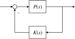
Figure 1: Standard feedback control structure

Then if $P(s)$ is perturbed by uncertainties in the form of gain or phase within a sufficiently small range, by continuity, the controller $K(s)$ still stabilizes the perturbed plant. But how large a perturbation in gain or phase can be tolerated before the feedback system becomes unstable?

Gain/phase margin maximization provides a quantitative answer to the above question. Following [7, Chapter 11], consider the family of plants

$${\mathscr{P}_{\mu}}=\left\{{\alpha P\left(s\right)\begin{array}[]{*{20}{c}}:&{1\leq\alpha<\mu}\end{array}}\right\}.$$ (2)

This represents uncertainty in the gain about the nominal plant model $P(s)$, and thereby, the maximal gain margin for $P(s)$,

$$\begin{array}[]{l}{k_{\scriptscriptstyle{\it M}}}=\sup\{\mu:\exists K\left(s\right)\mbox{ stabilizing }\alpha P\left(s\right),\;{\rm{}}\;\forall\alpha\in[1,\mu)\},\end{array}$$

specifies the largest family $\mathscr{P}_{k_{\scriptscriptstyle{\it M}}}$ that can be stabilized by the same LTI controller. Likewise, consider the family

$${\mathcal{Q}_{\nu}}=\left\{{{e^{-j\theta}}P\left(s\right)\begin{array}[]{*{20}{c}}:&{\theta\in(-\nu,\nu)}\end{array}}\right\},$$ (3)

and define the maximal phase margin

$$\begin{array}[]{l}{\theta_{\scriptscriptstyle{\it M}}}=\sup\{\nu:\exists K\left(s\right)\mbox{ stabilizing }{e^{-j\theta}}P\left(s\right),{\rm{}}\;\forall\theta\in(-\nu,\nu)\},\end{array}$$

which specifies the largest family $\mathcal{Q}_{\theta_{\scriptscriptstyle{\it M}}}$ stabilizable by the same suitably chosen LTI controller.

Remark 2.1: The definition of gain margin above and in [7, Chapter 11] serves some notational convenience, whereas a more practical definition would place the nominal plant in the (logarithmic) center of the parametric uncertainty, precisely as in [1, 2, 4], requiring that a controller stabilizes a maximal family $\{\alpha P(s):\sqrt{\mu^{-1}}<\alpha<\sqrt{\mu}\}$. Indeed, optimizing for a one-sided perturbation of the gain necessitates that an $\epsilon$-suboptimal controller stabilizes gain perturbation in an interval $1-\epsilon\leq\alpha\leq k_{\scriptscriptstyle{\it M}}-\epsilon$, placing the nominal plant in a precarious spot rendering the feedback system fragile to perturbations in one of the two direction. This very point became a source of controversy [41] in that earlier authors raised a debateable issue of fragility as endemic to gain margin maximization. $\hfill\blacksquare$

Remark 2.2: At times, when no confusion arises, we may measure the gain margin in decibels (dB), i.e., referring to $20\log_{10}k_{\scriptscriptstyle{\it M}}$ as the maximal gain margin. $\hfill\blacksquare$

Define the system’s complementary sensitivity function by

$$T\left(s\right)=P\left(s\right)K\left(s\right){\left[{1+P\left(s\right)K\left(s\right)}\right]^{-1}},$$

and let

$${\gamma_{{\rm{opt}}}}=\inf\left\{{{{\left\|T(s)\right\|}_{\infty}}:\;K\left(s\right)\;{\rm{stabilizes}}\;P\left(s\right)}\right\},$$ (4)

with $\|T(s)\|_{\infty}$ being the $\mathcal{H}_{\infty}$-norm of $T(s)$. The following result due to Tannenbaum [1, 3] (see also [4, 7] for a lucid exposition) provides analytical expressions of $k_{\scriptscriptstyle{\it M}}$ and $\theta_{\scriptscriptstyle{\it M}}$ that can be determined by solving the standard $\mathcal{H}_{\infty}$ optimal control problem in (4).

Proposition 2.1: (i). If $P$ is stable or minimum-phase, then the maximal gain margin ${k_{\scriptscriptstyle{\it M}}}=\infty$. Otherwise,

$${k_{\scriptscriptstyle{\it M}}}={\left({\frac{{{\gamma_{{\rm{opt}}}}+1}}{{{\gamma_{{\rm{opt}}}}-1}}}\right)^{2}}.$$ (5)

(ii). If $P$ is stable or minimum-phase, then the maximal phase margin is ${\theta_{\scriptscriptstyle{\it M}}}=\pi$ (in radians). Otherwise,

$${\theta_{\scriptscriptstyle{\it M}}}=2{\sin^{-1}}\frac{1}{{{\gamma_{{\rm{opt}}}}}}.$$ (6)

The goal of the present paper is determine the maximal robustness margins that are achievable by PID controllers; that is, by controllers with transfer function of the form

$${K_{{\scriptscriptstyle{\it PID}}}}\left(s\right)={k_{p}}+\frac{{{k_{i}}}}{s}+{k_{d}}s.$$ (7)

Thus, accordingly, we define

$$\begin{array}[]{l}k_{\scriptscriptstyle{\it M}}^{{\scriptscriptstyle{\it PID}}}=\sup\{\mu:~{}\exists{K_{{\scriptscriptstyle{\it PID}}}}\left(s\right){\rm{\;stabilizing~{}}}\alpha P\left(s\right)\;\forall\alpha\in[1,\mu)\},\end{array}$$

$$\begin{array}[]{l}\theta_{\scriptscriptstyle{\it M}}^{{\scriptscriptstyle{\it PID}}}=\sup\{\nu:~{}\exists{K_{{\scriptscriptstyle{\it PID}}}}\left(s\right){\rm{\;stabilizing}}{e^{-j\theta}}P\left(s\right)\;\forall\theta\in(-\nu,\nu)\}.\end{array}$$

Likewise, it is of interest to consider subclasses of PID controllers, such as proportional, PI, and PD controllers, given by

$$\begin{array}[]{*{20}{cc}}\displaystyle{{K_{\scriptscriptstyle{\it P}}}\left(s\right)={k_{p}},}&\displaystyle K_{{\scriptscriptstyle{\it PI}}}(s)=k_{p}+\frac{k_{i}}{s},&\displaystyle{{K_{{\scriptscriptstyle{\it PD}}}}\left(s\right)={k_{p}}+{k_{d}}s},\end{array}$$ (8)

respectively. We shall denote the corresponding maximal gain and phase margins with the corresponding superscripts P, PI, and PD.

In our analysis, we only consider first- and second-order plants. This is partly due to the fact that industrial processes are often modeled by low-order, and in fact, mostly first-order and second-order systems, and partly due to the limitation of PID controllers in controlling high-order dynamics as, in general, PID controllers may not be able to stabilize certain third- and higher-order unstable systems [39, 36]. From a technical standpoint, unlike $k_{\scriptscriptstyle{\it M}}$ and $\theta_{\scriptscriptstyle{\it M}}$, computing maximal PID gain and phase margins requires solving a parametric optimization problem.

Our main results are summarized in Table 1, which provides analytical expressions of maximal gain and phase margins for first- and second-order plants. The rest of the paper is devoted to establishing these results and to the discussion of our findings.

Plants $P\left(s\right)$		Gain Margin $k_{\scriptscriptstyle{\it M}}^{{\scriptscriptstyle{\it PID}}}$	Phase Margin $\theta_{\scriptscriptstyle{\it M}}^{{\scriptscriptstyle{\it PID}}}$	Relation with ${k_{\scriptscriptstyle{\it M}}},{\theta_{\scriptscriptstyle{\it M}}}$
First-Order Systems	minimum-phase Plants	$\infty$	$\pi$	$\begin{array}[]{l}{k_{\scriptscriptstyle{\it M}}}=k_{\scriptscriptstyle{\it M}}^{{\scriptscriptstyle{\it PID}}}\\ {\theta_{\scriptscriptstyle{\it M}}}=\theta_{\scriptscriptstyle{\it M}}^{{\scriptscriptstyle{\it PID}}}\end{array}$
	$\frac{{s-z}}{{s-p}},~{}p,z>0$	${\max\left\{\frac{z}{p},~{}\frac{p}{z}\right\}}$	${\cos^{-1}}\left({\frac{{2\sqrt{z/p}}}{{1+\left({z/p}\right)}}}\right)$	$\begin{array}[]{l}{k_{\scriptscriptstyle{\it M}}}={(k_{\scriptscriptstyle{\it M}}^{{\scriptscriptstyle{\it PI}}})^{2}}\\ {\theta_{\scriptscriptstyle{\it M}}}=2\theta_{\scriptscriptstyle{\it M}}^{{\scriptscriptstyle{\it PI}}}\end{array}$
Second-Order Systems	minimum-phase Plants	$\infty$	$\pi$	$\begin{array}[]{l}{k_{\scriptscriptstyle{\it M}}}=k_{\scriptscriptstyle{\it M}}^{{\scriptscriptstyle{\it PID}}}\\ {\theta_{\scriptscriptstyle{\it M}}}=\theta_{\scriptscriptstyle{\it M}}^{{\scriptscriptstyle{\it PID}}}\end{array}$
	$\frac{{s-z}}{{\left({s-{p_{1}}}\right)\left({s-{p_{2}}}\right)}},~{}{p_{1}},{p_{2}},z>0$	explicit expression	analytical solution	$k_{\scriptscriptstyle{\it M}}^{{\scriptscriptstyle{\it PID}}}\leq{k_{\scriptscriptstyle{\it M}}}\leq{(k_{\scriptscriptstyle{\it M}}^{{\scriptscriptstyle{\it PID}}})^{2}}$

TABLE I: Stability Margins: Gain and Phase.

III First-Order Unstable Systems

In this section, we provide explicit expressions of maximal gain and phase margins of first-order systems achievable by PID controllers. The results show the dependence of these measures on the system’s unstable pole and nonminimum-phase zero.

We first consider first-order unstable plants described by

$$P\left(s\right)=\frac{{{\beta_{0}}s+{\beta_{1}}}}{{s-p}},\;\;p>0.$$ (9)

Without loss of generality, it is assumed that ${\beta_{0}}\geq 0$ and ${\beta_{1}}\neq 0$. Note that in the case ${\beta_{0}}\neq 0$, derivative control will result in an improper system. For this reason, in this section we shall focus on PI controllers.

Theorem 3.1: Let $P(s)$ be given by (9). Then the following statements hold:

(i). For ${\beta_{0}}>0$,

$$\begin{array}[]{*{20}{l}}{\kern-8.0pt}{k_{\scriptscriptstyle{\it M}}^{{\scriptscriptstyle{\it PI}}}=k_{\scriptscriptstyle{\it M}}^{\scriptscriptstyle{\it P}}=\left\{{\begin{array}[]{*{20}{l}}\displaystyle{{\max\left\{{\frac{{\left|{{\beta_{1}}}\right|/{\beta_{0}}}}{p},\frac{p}{{\left|{{\beta_{1}}}\right|/{\beta_{0}}}}}\right\},\;\;\;{\beta_{1}}<0,}}\\ \displaystyle{\infty,\;\;\;\;\;\;\;\;\;\;\;\;\;\;\;\;\;\;\;\;\;\;\;\;\;\;\;\;\;\;\;\;\;\;\;\;\;\;\;\,{\beta_{1}}>0.}\end{array}}\right.}\\ {\kern-8.0pt}{\theta_{\scriptscriptstyle{\it M}}^{{\scriptscriptstyle{\it PI}}}=\theta_{\scriptscriptstyle{\it M}}^{\scriptscriptstyle{\it P}}=\left\{{\begin{array}[]{*{20}{l}}\displaystyle{{{\cos}^{{\rm{-}}1}}\frac{{2\sqrt{{\beta_{0}}\left|{{\beta_{1}}}\right|/p}}}{{{\beta_{0}}+(\left|{{\beta_{1}}}\right|/p)}},\;\;\;\;\;\;\;\;\;\;\;\;\;\,{\beta_{1}}<0,}\\ \displaystyle{\pi,\;\;\;\;\;\;\;\;\;\;\;\;\;\;\;\;\;\;\;\;\;\;\;\;\;\;\;\;\;\;\;\;\;\;\;\;\;\;\;\;\;\,{\beta_{1}}>0.}\end{array}}\right.}\end{array}$$ (10)

(ii). For ${\beta_{0}}=0$,

$$\begin{array}[]{l}{\kern-126.0pt}k_{\scriptscriptstyle{\it M}}^{{\scriptscriptstyle{\it PID}}}=k_{\scriptscriptstyle{\it M}}^{{\scriptscriptstyle{\it PD}}}=k_{\scriptscriptstyle{\it M}}^{\scriptscriptstyle{\it P}}=\infty,\\ {\kern-126.0pt}\theta_{\scriptscriptstyle{\it M}}^{{\scriptscriptstyle{\it PID}}}=\theta_{\scriptscriptstyle{\it M}}^{{\scriptscriptstyle{\it PD}}}=2\theta_{\scriptscriptstyle{\it M}}^{\scriptscriptstyle{\it P}}=\pi.\end{array}$$ (11)

Proof: See Appendix B. $\hfill\blacksquare$

The expressions given in Theorem 3.1 lead us to a number of pertinent observations. First, it is clear that integral control has no effect on maximizing either the gain or the phase margin. This is consistent with one’s intuition; integral control has its essential utility in tracking reference signals. Secondly, we note that for minimum-phase plants (${\beta_{0}}>0$ and ${\beta_{1}}>0$) of relative degree zero, proportional control suffices to achieve the maximum possible infinite gain margin and a phase margin of $\pm{180^{\circ}}$. For nonminimum-phase plants (${\beta_{0}}>0$ and ${\beta_{1}}<0$), it is instructive to consider

$$P\left(s\right)=\frac{{s-z}}{{s-p}},\;\;\;\;p>0,\;\;z>0.$$ (12)

In this case, it follows from Theorem 3.1 that

$$\begin{array}[]{l}\displaystyle{k_{\scriptscriptstyle{\it M}}^{{\scriptscriptstyle{\it PI}}}=k_{\scriptscriptstyle{\it M}}^{\scriptscriptstyle{\it P}}=\max\left\{{\frac{z}{p},~{}\frac{p}{z}}\right\}}.\\ \displaystyle{\theta_{\scriptscriptstyle{\it M}}^{{\scriptscriptstyle{\it PI}}}=\theta_{\scriptscriptstyle{\it M}}^{\scriptscriptstyle{\it P}}={\cos^{{\rm{-}}1}}\frac{{2\sqrt{z/p}}}{{1+\left({z/p}\right)}}}.\end{array}$$ (13)

It is interesting to see that

$$\theta_{\scriptscriptstyle{\it M}}^{{\scriptscriptstyle{\it PI}}}=\theta_{\scriptscriptstyle{\it M}}^{\scriptscriptstyle{\it P}}={\cos^{-1}}\frac{{2\sqrt{k_{\scriptscriptstyle{\it M}}^{\scriptscriptstyle{\it P}}}}}{{1+k_{\scriptscriptstyle{\it M}}^{\scriptscriptstyle{\it P}}}}={\cos^{-1}}\frac{{2\sqrt{k_{\scriptscriptstyle{\it M}}^{{\scriptscriptstyle{\it PI}}}}}}{{1+k_{\scriptscriptstyle{\it M}}^{{\scriptscriptstyle{\it PI}}}}}.$$ (14)

We conclude this section with a comparison of the maximal gain and phase margins herein with those achievable by the general LTI controllers. The following corollary states that for a first-order nonminimum-phase plant, the maximal gain and phase margins achievable by a proportional controller are half as good as those by general LTI controllers.

Corollary 3.1: Let $P(s)$ be given by (12). Then

$$\begin{array}[]{l}{\log_{10}}{k_{\scriptscriptstyle{\it M}}}~{}~{}=~{}~{}2{\log_{10}}k_{\scriptscriptstyle{\it M}}^{{\scriptscriptstyle{\it PI}}}~{}~{}=~{}~{}2{\log_{10}}k_{\scriptscriptstyle{\it M}}^{\scriptscriptstyle{\it P}}.\\ {\theta_{\scriptscriptstyle{\it M}}}~{}~{}~{}~{}~{}\;\,~{}~{}=~{}~{}2\theta_{\scriptscriptstyle{\it M}}^{{\scriptscriptstyle{\it PI}}}~{}~{}~{}~{}~{}~{}\,~{}~{}=~{}~{}2\theta_{\scriptscriptstyle{\it M}}^{\scriptscriptstyle{\it P}}.\end{array}$$ (15)

Proof: With $P(s)$ given by (12), it follows from [42] (see also [4]) that

$${\gamma_{{\rm{opt}}}}=\left|{\frac{{z+p}}{{z-p}}}\right|.$$

Invoking Proposition 2.1 yields

$${k_{\scriptscriptstyle{\it M}}}=\max\left\{\left({\frac{z}{p}}\right)^{2},~{}\left({\frac{p}{z}}\right)^{2}\right\},$$

$${\theta_{\scriptscriptstyle{\it M}}}=2{\cos^{{\rm{-}}1}}\frac{{2\sqrt{z/p}}}{{1+\left({z/p}\right)}}.$$

In view of (13), the corollary follows. $\hfill\blacksquare$

IV Second-Order Unstable Systems

This section presents results for second-order unstable plants, which include minimum-phase as well as nonminimum-phase systems. In general, the computation of the gain and phase margins for second-order plants poses a more difficult problem. Throughout this section, our development seeks to recast the gain and phase maximization problems as one of nonlinear programming. For their essential flavor, we employ the KKT condition to obtain value of the integral gain as the necessary solution to the nonlinear programming problems under consideration, which show that unequivocally in all cases, the optimal integral gain is $k_{i}=0$. The maximal gain and phase margins are then obtained by solving a univariate optimization problem, defined in terms of a function of the proportional gain $k_{p}$ or the derivative gain $k_{d}$ alone.

IV-A Minimum-phase Systems

We begin with minimum-phase plants that contain a pair of unstable poles ${p_{1}}$, ${p_{2}}$, described by

$$P\left(s\right)=\frac{{{\beta_{0}}s+{\beta_{1}}}}{{\left({s-{p_{1}}}\right)\left({s-{p_{2}}}\right)}},\;\;{\mathop{\rm Re}\nolimits}\left({{p_{1}}}\right)>0,\;\;{\mathop{\rm Re}\nolimits}\left({{p_{2}}}\right)>0,$$ (16)

where ${\beta_{0}}\geq 0,{\beta_{1}}>0$. To ensure that $P\left(s\right)$ is a real rational plant, we assume that ${p_{1}}$ and ${p_{2}}$ are either real poles or form a complex conjugate pair.

Theorem 4.1: Let $P(s)$ be given by (16). Then the following statements hold:

(i).

$$\begin{array}[]{l}k_{\scriptscriptstyle{\it M}}^{\scriptscriptstyle{\it P}}=\left\{{\begin{array}[]{*{20}{l}}{{\rm{none}},\;\;\;{\rm{when}}\;{\beta_{0}}=0},\\ {\infty,\;\;\;\;\;\;\;{\rm{when}}\;{\beta_{0}}\neq 0.}\end{array}}\right.\\ k_{\scriptscriptstyle{\it M}}^{{\scriptscriptstyle{\it PID}}}=k_{\scriptscriptstyle{\it M}}^{{\scriptscriptstyle{\it PD}}}=\infty.\end{array}$$ (17)

(ii).

$$\begin{array}[]{l}\theta_{\scriptscriptstyle{\it M}}^{\scriptscriptstyle{\it P}}=\left\{{\begin{array}[]{*{20}{l}}{{\rm{none}},\;\;\;{\rm{when}}\;{\beta_{0}}=0,}\\ {\pi/2,\;\;\;\;\;\;\;\;{\rm{when}}\;{\beta_{0}}\neq 0.}\end{array}}\right.\\ \theta_{\scriptscriptstyle{\it M}}^{{\scriptscriptstyle{\it PID}}}=\theta_{\scriptscriptstyle{\it M}}^{{\scriptscriptstyle{\it PD}}}=\left\{{\begin{array}[]{*{20}{l}}{\pi/2,\;\;\;{\rm{when}}\;{\beta_{0}}=0,}\\ {\pi,\;\;\;\;{\rm{when}}\;{\beta_{0}}\neq 0.}\end{array}}\right.\end{array}$$ (18)

Proof: The proof follows analogously as in that of Theorem 3.1, and hence is omitted. $\hfill\blacksquare$

It is clear from Theorem 4.1 that for second-order systems the maximal gain and phase margins achievable by PID control are the same as those by general LTI controllers, provided that the plant is minimum-phase and has a relative degree no greater than one. On the other hand, if the plant does have a relative degree greater than one, then the maximal phase margin is reduced to ${\pi}/{2}$, despite the fact that the maximal gain margin remains unchanged.

IV-B Nonminimum-phase Systems

One of our primary results in this paper pertains to second-order unstable, nonminimum-phase plants. We consider specifically the plant described by

$${\kern-5.0pt}P\left(s\right)\!=\!\frac{{s-z}}{{\left({s\!-\!{p_{1}}}\right)\left({s\!-\!{p_{2}}}\right)}},\;\;{\mathop{\rm Re}\nolimits}\left({{p_{1}}}\right)>0,\;\;{\mathop{\rm Re}\nolimits}\left({{p_{2}}}\right)>0,$$ (19)

where likewise, $z>0$, ${p_{1}}$ and ${p_{2}}$ are either real or are a complex conjugate pair. To facilitate our development, we introduce the functions

$${\kern 0.0pt}\hat{\theta}\left({{k_{p}}}\right)={\tan^{-1}}\frac{{({{p_{1}}+{p_{2}}})\hat{\omega}({k_{p}})}}{{{p_{1}}{p_{2}}-{\hat{\omega}^{2}}({k_{p}})}}-{\tan^{-1}}\frac{{\hat{\omega}({k_{p}})}}{z}-{\tan^{-1}}\frac{{\hat{\omega}({k_{p}})}}{{{k_{p}}}},$$ (20)

and

$$\begin{array}[]{l}{\kern-15.0pt}\displaystyle\tilde{\theta}\left({{k_{d}}}\right)=\pi-{\tan^{-1}}\frac{{({{p_{1}}+{p_{2}}})\tilde{\omega}({k_{d}})}}{{{\tilde{\omega}^{2}}({k_{d}})-{p_{1}}{p_{2}}}}\\ {\kern 60.0pt}\displaystyle-{\tan^{-1}}\frac{{\tilde{\omega}({k_{d}})}}{z}+{\tan^{-1}}\frac{{z{k_{d}}\tilde{\omega}({k_{d}})}}{{{p_{1}}{p_{2}}}},\end{array}$$ (21)

where

$$\hat{\omega}(k_{p})=\sqrt{\frac{{p_{1}^{2}p_{2}^{2}-{z^{2}}k_{p}^{2}}}{k_{p}^{2}+{z^{2}}-p_{1}^{2}-p_{2}^{2}}},$$ (22)

$$\tilde{\omega}({k_{d}})=\sqrt{\frac{{{z^{2}}k_{d}^{2}+{{\left({{p_{1}}{p_{2}}/z}\right)}^{2}}-p_{1}^{2}-p_{2}^{2}}}{{1-k_{d}^{2}}}}.$$ (23)

We first present the following theorem for plants with two real unstable poles.

Theorem 4.2 (Real Poles): Let $P(s)$ be given by (19), and $p_{1},~{}p_{2}$ be real poles. For ${K_{{\scriptscriptstyle{\it PD}}}}\left(s\right)$ and ${K_{{\scriptscriptstyle{\it PID}}}}\left(s\right)$ to stabilize $P(s)$, it is necessary that $({p_{1}}-z)({p_{2}}-z)\neq 0$. Under this condition, the following statements hold:

(i). Gain Margin: For $({p_{1}}-z)({p_{2}}-z)>0$,

$${\kern-4.0pt}\displaystyle k_{\scriptscriptstyle{\it M}}^{{\scriptscriptstyle{\it PID}}}=k_{\scriptscriptstyle{\it M}}^{{\scriptscriptstyle{\it PD}}}=\left\{\begin{array}[]{ll}\displaystyle{\kern-8.0pt}\frac{p_{1}p_{2}}{z({p_{1}}+{p_{2}})-z^{2}},&\mbox{if~{}}z<\min\{{p_{1}},{p_{2}}\},\\ \displaystyle{\kern-8.0pt}\frac{z^{2}}{z({p_{1}}+{p_{2}})-{p_{1}}{p_{2}}}&\mbox{if~{}}z>\max\{{p_{1}},{p_{2}}\}.\end{array}\right.$$ (24)

Otherwise, for $({p_{1}}-z)({p_{2}}-z)<0$,

$${\kern-2.0pt}\displaystyle k_{\scriptscriptstyle{\it M}}^{{\scriptscriptstyle{\it PID}}}=k_{\scriptscriptstyle{\it M}}^{{\scriptscriptstyle{\it PD}}}=\left\{{\begin{array}[]{*{20}{l}}\displaystyle{\kern-8.0pt}\frac{{z({p_{1}}\!+\!{p_{2}})\!-\!{z^{2}}}}{{{p_{1}}{p_{2}}}},\;\;\;\,{\rm{if}}\;\min\{{p_{1}},{p_{2}}\}<z\leq\sqrt{{p_{1}}{p_{2}}},\\ \displaystyle{\kern-6.0pt}\frac{{z({p_{1}}\!+\!{p_{2}})\!-\!{p_{1}}{p_{2}}}}{{{z^{2}}}},{\rm{if}}\;\sqrt{{p_{1}}{p_{2}}}<z<\max\{{p_{1}},{p_{2}}\}.\end{array}}\right.$$ (25)

(ii). Phase Margin: For $({p_{1}}-z)({p_{2}}-z)>0$,

$$\theta_{\scriptscriptstyle{\it M}}^{{\scriptscriptstyle{\it PID}}}=\theta_{\scriptscriptstyle{\it M}}^{{\scriptscriptstyle{\it PD}}}=\left\{\begin{array}[]{ll}|{\hat{\theta}({{\hat{k}}_{p}})}|,&{\rm{if}}\;z<\min\{{p_{1}},{p_{2}}\},\\ \tilde{\theta}({{\tilde{k}}_{d}}),&{\rm{if}}\;z>\max\{{p_{1}},{p_{2}}\},\end{array}\right.$$ (26)

where ${\hat{k}_{p}}\in({p_{1}}+{p_{2}}-z,\;{p_{1}}{p_{2}}/z)$ is the unique positive solution to the polynomial equation

$$k_{p}^{3}+{c_{2}}k_{p}^{2}+{c_{1}}{k_{p}}+{c_{0}}=0$$ (27)

with coefficients

$${c_{2}}={p_{1}}+{p_{2}}-z,$$

$${c_{1}}=(z-{p_{1}}-{p_{2}}){p_{1}}{p_{2}}/z,$$ (28)

$${c_{0}}=({z^{2}}-p_{1}^{2}-p_{2}^{2}){p_{1}}{p_{2}}/z,$$

and ${{\tilde{k}}_{d}}\in(-1,\;({p_{1}}{p_{2}}/{z^{2}})-(({p_{1}}+{p_{2}})/z))$ is the unique negative solution to the polynomial equation

$$k_{d}^{3}+{d_{2}}k_{d}^{2}+{d_{1}}{k_{d}}+{d_{0}}=0$$ (29)

with coefficients

$$\begin{array}[]{l}{d_{2}}={d_{1}}=({p_{1}}{p_{2}}-({p_{1}}+{p_{2}})z)/{z^{2}},\\ {d_{0}}=(p_{1}^{2}+p_{2}^{2}-{({p_{1}}{p_{2}}/z)^{2}})/{z^{2}}.\end{array}$$ (30)

Otherwise, for $({p_{1}}-z)({p_{2}}-z)<0$,

$${\kern-6.0pt}\theta_{\scriptscriptstyle{\it M}}^{{\scriptscriptstyle{\it PID}}}=\theta_{\scriptscriptstyle{\it M}}^{{\scriptscriptstyle{\it PD}}}=\max\{\hat{\theta}({{\hat{k}}_{p}}),|{\tilde{\theta}({{\tilde{k}}_{d}})}|\},$$ (31)

where ${{\hat{k}}_{p}}\in({p_{1}}{p_{2}}/z,\;{p_{1}}+{p_{2}}-z)$ is the unique solution to the equation (27), and ${{\tilde{k}}_{d}}\in(({p_{1}}{p_{2}}/{z^{2}})-(({p_{1}}+{p_{2}})/z),\;-1)$ is the unique solution to the equation (29).

Proof: See Appendix C. $\hfill\blacksquare$

The following theorem is a counterpart to Theorem 4.2 for plants with complex conjugate poles. While the result is essentially similar, subtle differences do exist. For example, for a pair of complex conjugate poles $p_{1}=p$ and $p_{2}=p^{*}$, it always holds that $({p_{1}}-z)({p_{2}}-z)=|p-z|^{2}>0$, while on the contrary the case $({p_{1}}-z)({p_{2}}-z)<0$ is precluded. For this reason, we state the result separately.

Theorem 4.3 (Complex Poles): Let $P(s)$ be given by (19), and ${p_{1}}=p=\sigma+j\nu$, ${p_{2}}={p^{*}}=\sigma-j\nu$ with $\sigma>0$. Then, the following statements hold:

(i). Gain Margin: For $\left|{p-z}\right|<z$,

$${\kern-9.0pt}\displaystyle k_{\scriptscriptstyle{\it M}}^{{\scriptscriptstyle{\it PID}}}=k_{\scriptscriptstyle{\it M}}^{{\scriptscriptstyle{\it PD}}}=\left\{{\begin{array}[]{*{20}{l}}\displaystyle{\frac{{{p_{1}}{p_{2}}}}{{z({p_{1}}\!+\!{p_{2}})\!-\!{z^{2}}}},\;\;\;\;\;\;\;\;\;\;{\rm{if}}\;z\leq\left|p\right|,}\\ \displaystyle{\frac{{{z^{2}}}}{{z({p_{1}}\!+\!{p_{2}})\!-\!{p_{1}}{p_{2}}}},\;\;\;\;\;\;\;{\rm{if}}\;z>\left|p\right|.}\end{array}}\right.$$ (32)

Otherwise, for $\left|{p-z}\right|\geq z$,

$${\kern-9.0pt}\displaystyle k_{\scriptscriptstyle{\it M}}^{{\scriptscriptstyle{\it PID}}}=k_{\scriptscriptstyle{\it M}}^{{\scriptscriptstyle{\it PD}}}=\left\{{\begin{array}[]{*{20}{l}}\displaystyle{\frac{{{p_{1}}{p_{2}}}}{{z({p_{1}}+{p_{2}})-{z^{2}}}},\;\;\,{\rm{if}}\;z<{p_{1}}+{p_{2}},}\\ \displaystyle{\frac{{{p_{1}}{p_{2}}+{z^{2}}}}{{z({p_{1}}+{p_{2}})}},\;\;\;\;\;\;\;\;\;\;\,{\rm{if}}\;z\geq{p_{1}}+{p_{2}}.}\end{array}}\right.$$ (33)

(ii). Phase Margin: For $\left|{p-z}\right|<z$,

$${\kern-12.0pt}\theta_{\scriptscriptstyle{\it M}}^{{\scriptscriptstyle{\it PID}}}=\theta_{\scriptscriptstyle{\it M}}^{{\scriptscriptstyle{\it PD}}}=\left\{{\begin{array}[]{*{20}{l}}{|\hat{\theta}({{\hat{k}}_{p}})|,\;\;\;\;\;\;\;\;\;\;\;\;\;{\rm{if}}\;z\leq\left|p\right|,}\\ {\tilde{\theta}({{\tilde{k}}_{d}}),\;\;\;\;\;\;\;\;\;\;\;\;\;\;\;{\rm{if}}\;z>\left|p\right|.}\end{array}}\right.$$ (34)

Otherwise, for $\left|{p-z}\right|\geq z$,

$$\theta_{\scriptscriptstyle{\it M}}^{{\scriptscriptstyle{\it PID}}}=\theta_{\scriptscriptstyle{\it M}}^{{\scriptscriptstyle{\it PD}}}=|\hat{\theta}({{\hat{k}}_{p}})|,$$ (35)

where ${\hat{k}_{p}}\in({p_{1}}+{p_{2}}-z,\;{p_{1}}{p_{2}}/z)$ is the unique solution to the polynomial equation (27), and ${{\tilde{k}}_{d}}\in(-1,\;({p_{1}}{p_{2}}/{z^{2}})-(({p_{1}}+{p_{2}})/z))$ is the unique solution to the polynomial equation (29).

Proof: See Appendix D. $\hfill\blacksquare$

Remark 4.1: It is worth noting that, while given in terms of the positive real roots of polynomials, both $\hat{k}_{p}$ and $\tilde{k}_{d}$ can be calculated explicitly using the classical Cardano formula [43]. In this sense, the expressions for the phase margin (i.e., (26)-(31), and (34)-(34)) provide in fact analytical solutions to the phase maximization problem. Furthermore, note also that because of the uniqueness of the solutions, the functions $\hat{\theta}(k_{p})$ and $\tilde{\theta}(k_{d})$ define, respectively, unimodal convex and concave functions on the corresponding intervals, a fact further evidenced by the following example.

Example 4.1: In this example, we compare the maximal margins achievable by PID controllers and those by general LTI controllers. We consider plants with both real poles and complex conjugate poles specified as follows.

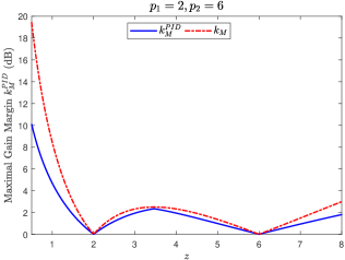
Figure 2: Maximal gain margin $k_{\scriptscriptstyle{\it M}}^{{\scriptscriptstyle{\it PID}}}$ of the system (19) vs. ${k_{\scriptscriptstyle{\it M}}}$ : Real poles.

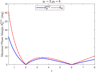
Figure 3: Maximal phase margin $\theta_{\scriptscriptstyle{\it M}}^{{\scriptscriptstyle{\it PID}}}$ of the system (19) vs. ${\theta_{\scriptscriptstyle{\it M}}}$ : Real poles.

Real unstable poles ${p_{1}}>0,{p_{2}}>0$: In this case we take ${p_{1}}=2$, ${p_{2}}=6$ and let $z$ vary in the interval $\left[{0.5,{\rm{}}8}\right]$. Fig. 2 plots the gain margins $20{\log_{10}}k_{\scriptscriptstyle{\it M}}^{{\scriptscriptstyle{\it PID}}}$ and $20{\log_{10}}{k_{\scriptscriptstyle{\it M}}}$ (both in db) as functions of $z$, and Fig. 3 presents the phase margins $\theta_{\scriptscriptstyle{\it M}}^{{\scriptscriptstyle{\it PID}}}$ and $\theta_{\scriptscriptstyle{\it M}}$ (in deg) as functions of $z$. Note that, when $z=p_{1}$ or $z=p_{2}$, the gain and phase margins both vanish.

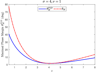
Figure 5: Maximal phase margin $\theta_{\scriptscriptstyle{\it M}}^{{\scriptscriptstyle{\it PID}}}$ of the system (19) vs. ${\theta_{\scriptscriptstyle{\it M}}}$ : Complex poles.

Complex conjugate unstable poles ${p_{1}}=\sigma+j\nu,{p_{2}}=\sigma-j\nu$: We take $\sigma=4$, $\nu=1$ and let $z$ vary in the interval $\left[{0.5,{\rm{}}8}\right]$. Fig. 4 shows the gain margins $20{\log_{10}}k_{\scriptscriptstyle{\it M}}^{{\scriptscriptstyle{\it PID}}}$ and $20{\log_{10}}{k_{\scriptscriptstyle{\it M}}}$, while Fig. 5 describes the phase margins $\theta_{\scriptscriptstyle{\it M}}^{{\scriptscriptstyle{\it PID}}}$ and $\theta_{\scriptscriptstyle{\it M}}$.

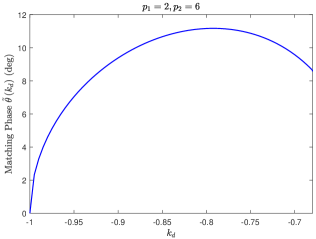
Figure 6: The phase $\tilde{\theta}\left({{k_{d}}}\right)$ of the system (19): $z>\max{\rm{\{}}{p_{1}},{p_{2}}{\rm{\}}}$.

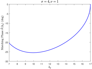
Figure 7: The phase $\hat{\theta}\left({{k_{p}}}\right)$ of the system (19): $\left|{p-z}\right|\geq z$.

To facilitate the understanding of Theorem 4.2-4.3 and their proofs, we also plot $\hat{\theta}\left({{k_{p}}}\right)$ and $\tilde{\theta}\left({{k_{d}}}\right)$. Fig. 6 corresponds to the case $z>\max{\rm{\{}}{p_{1}},{p_{2}}{\rm{\}}}$ (herein $z=10$), where we observe that $\tilde{\theta}\left({{k_{d}}}\right)>0$ in $\left({-1,-0.68}\right)$, where $\tilde{\theta}(k_{d})$ is concave and has a unique maximum. Fig. 7 demonstrates that for $\left|{p-z}\right|\geq z$ (herein $z=1$), $\hat{\theta}\left({{k_{p}}}\right)<0$ in $\left({7,17}\right)$, indicating that in this interval, $\hat{\theta}\left({{k_{p}}}\right)$ is convex and admits a unique minimum. $\hfill\blacksquare$

Interestingly, by a careful inspection, we observe further from the gain margin plots that the ratio ${\log_{10}}{k_{\scriptscriptstyle{\it M}}}/{\log_{10}}k_{\scriptscriptstyle{\it M}}^{{\scriptscriptstyle{\it PID}}}$ seemingly is within a factor of two. This, in fact, turns out not to be a coincidence. The following corollary shows that, as with first-order plants, ${\log_{10}}{k_{\scriptscriptstyle{\it M}}}$ is always within a factor of two of ${\log_{10}}k_{\scriptscriptstyle{\it M}}^{{\scriptscriptstyle{\it PID}}}$.

Corollary 4.1: Let $P(s)$ be given by (19). Then,

$${\log_{10}}k_{\scriptscriptstyle{\it M}}^{{\scriptscriptstyle{\it PID}}}\leq{\log_{10}}{k_{\scriptscriptstyle{\it M}}}\leq 2{\log_{10}}k_{\scriptscriptstyle{\it M}}^{{\scriptscriptstyle{\it PID}}}.$$ (36)

Proof: We consider the case of real poles. The proof for the case of complex poles follows analogously and hence is omitted. Note from [42] that for $P(s)$ given by (19),

$${\gamma_{{\rm{opt}}}}=\prod\limits_{i=1}^{2}{\left|{\frac{{{p_{i}}+z}}{{{p_{i}}-z}}}\right|},$$

which can be written explicitly as

$$\gamma_{opt}=\displaystyle{\left\{\begin{array}[]{ll}\frac{(p_{1}+z)(p_{2}+z)}{(z-p_{1})(p_{2}-z)}&\mbox{~{}if ~{}}p_{1}<z<p_{2},\\ \frac{(p_{1}+z)(p_{2}+z)}{(p_{1}-z)(p_{2}-z)}&\mbox{~{}otherwise.}\end{array}\right.}$$

Accordingly,

$$\sqrt{k_{\scriptscriptstyle{\it M}}}=\frac{\gamma_{opt}+1}{\gamma_{opt}-1}=\displaystyle{\left\{\begin{array}[]{ll}\frac{z(p_{1}+p_{2})}{z^{2}+p_{1}p_{2}}&\mbox{~{}if ~{}}p_{1}<z<p_{2},\\ \frac{z^{2}+p_{1}p_{2}}{z(p_{1}+p_{2})}&\mbox{~{}otherwise.}\end{array}\right.}$$

Note also that under the condition $({p_{1}}-z)({p_{2}}-z)<0$, it holds that

$$\frac{{z({p_{1}}+{p_{2}})}}{{{z^{2}}+{p_{1}}{p_{2}}}}\leq\frac{{z({p_{1}}+{p_{2}})-{z^{2}}}}{{{p_{1}}{p_{2}}}},$$

$$\frac{{z({p_{1}}+{p_{2}})}}{{{z^{2}}+{p_{1}}{p_{2}}}}\leq\frac{{z({p_{1}}+{p_{2}})-{p_{1}}{p_{2}}}}{{{z^{2}}}}.$$

On the other hand, it is straightforward to verify that

$$\frac{z^{2}+p_{1}p_{2}}{z(p_{1}+p_{2})}\leq\frac{z^{2}}{z(p_{1}+p_{2})-p_{1}p_{2}},$$

and

$$\frac{z^{2}+p_{1}p_{2}}{z(p_{1}+p_{2})}\leq\frac{p_{1}p_{2}}{z(p_{1}+p_{2})-z^{2}},$$

provided that $({p_{1}}-z)({p_{2}}-z)>0$, or equivalently, $p_{1}+p_{2}-z<p_{1}p_{2}/z$. Thus, in all cases, it holds that $\sqrt{k_{\scriptscriptstyle{\it M}}}\leq k^{{\scriptscriptstyle{\it PID}}}_{\scriptscriptstyle{\it M}}$. This concludes the proof for the inequalities in (36). $\hfill\blacksquare$

Remark 4.2: From the numerical results in Fig. 3 and Fig. 5, it appears plausible to contend that a similar relationship holds for the phase margins $\theta_{\scriptscriptstyle{\it M}}^{{\scriptscriptstyle{\it PID}}}$ and $\theta_{M}$; that is,

$$\theta_{\scriptscriptstyle{\it M}}^{{\scriptscriptstyle{\it PID}}}\leq{\theta_{\scriptscriptstyle{\it M}}}\leq 2\theta_{\scriptscriptstyle{\it M}}^{{\scriptscriptstyle{\it PID}}}.$$ (37)

While a general proof is currently unavailable, it can be shown that under certain circumstances, the inequality does hold. Consider for example, the case $z<\min\{{p_{1}},{p_{2}}\}$. It follows instantly from Proposition 2.1 that

$${\tan}\frac{{{\theta_{\scriptscriptstyle{\it M}}}}}{2}=\frac{{({p_{1}}-z)({p_{2}}-z)}}{{2\sqrt{z({p_{1}}+{p_{2}})({p_{1}}{p_{2}}-{z^{2}})}}}.$$

Hence, to establish the inequality ${\theta_{\scriptscriptstyle{\it M}}}\leq 2\theta_{\scriptscriptstyle{\it M}}^{{\scriptscriptstyle{\it PID}}}$, it is both necessary and sufficient to show that

$${\tan}\frac{\theta_{\scriptscriptstyle{\it M}}}{2}\leq{\tan}|\hat{\theta}({\hat{k}_{p}})|.$$

We evaluate instead $\hat{\theta}(p_{1}+p_{2}-z)$, and find conditions such that $\theta_{\scriptscriptstyle{\it M}}\leq 2|\hat{\theta}(p_{1}+p_{2}-z)|$. By algebraic manipulation, we obtain

$$\begin{array}[]{l}\displaystyle{\kern-8.0pt}|\hat{\theta}({k_{p}})|=\pi-{\tan^{-1}}\frac{{({p_{1}}+{p_{2}})\hat{\omega}({k_{p}})}}{{{p_{1}}{p_{2}}-{\hat{\omega}^{2}}({k_{p}})}}-{\tan^{-1}}\frac{{({k_{p}}+z)\hat{\omega}({k_{p}})}}{{{\hat{\omega}^{2}}({k_{p}})-{k_{p}}z}}.\end{array}$$

At ${k_{p}}={p_{1}}+{p_{2}}-z$, we have

$$|\hat{\theta}(p_{1}+p_{2}-z)|={\tan^{-1}}\frac{({p_{1}}+{p_{2}})({p_{1}}{p_{2}}-{k_{p}}z)\bar{\omega}}{({p_{1}}+{p_{2}})^{2}\bar{\omega}^{2}-({p_{1}}{p_{2}}-\bar{\omega}^{2})^{2}},$$

where

$$\bar{\omega}=\hat{\omega}(p_{1}+p_{2}-z)=\sqrt{\frac{p_{1}p_{2}+z(p_{1}+p_{2}-z)}{2}~{}},$$ (38)

and ${p_{1}}{p_{2}}-{k_{p}}z=(p_{1}-z)(p_{2}-z)$. To show that $\theta_{\scriptscriptstyle{\it M}}\leq 2|\hat{\theta}(p_{1}+p_{2}-z)|$, it suffices to prove that $\tan(\theta_{\scriptscriptstyle{\it M}}/2)\leq\tan|\hat{\theta}(p_{1}+p_{2}-z)|$, which is equivalent to the condition

$$\begin{array}[]{l}{\kern-25.0pt}2({p_{1}}+{p_{2}})\bar{\omega}\sqrt{z({p_{1}}+{p_{2}})({p_{1}}{p_{2}}-{z^{2}})}\\ {\kern 25.0pt}\geq({p_{1}}+{p_{2}})^{2}\bar{\omega}^{2}-({p_{1}}{p_{2}}-\bar{\omega}^{2})^{2}.\end{array}$$ (39)

It can be readily verified, however, that this inequality holds whenever

$$\frac{{{p_{1}}+{p_{2}}}}{z}\leq 4\frac{{{p_{1}}{p_{2}}+{z^{2}}}}{{{p_{1}}{p_{2}}+z({p_{1}}+{p_{2}}-z)}}.$$ (40)

Consequently, in the case $z<\min\{{p_{1}},{p_{2}}\}$, under the condition (40), we have found that

$$\theta_{\scriptscriptstyle{\it M}}\leq 2|\hat{\theta}(p_{1}+p_{2}-z)|\leq 2\theta_{\scriptscriptstyle{\it M}}^{{\scriptscriptstyle{\it PID}}}.$$

In fact, since $|\hat{\theta}(p_{1}+p_{2}-z)|$ can be significantly smaller than $\theta_{\scriptscriptstyle{\it M}}^{{\scriptscriptstyle{\it PID}}}$, the analysis reveals, even more strikingly, that $\theta_{\scriptscriptstyle{\it M}}^{{\scriptscriptstyle{\it PID}}}$ can be much closer to $\theta_{\scriptscriptstyle{\it M}}$ than within a factor of two. $\hfill\blacksquare$

Equally of interest, the following corollary suggests that in the presence of a nonminimum-phase zero, the maximal phase margin attainable by PID control is limited to $90^{0}$, thus also highlighting the limitation of PID controllers.

Corollary 4.2: Let $P(s)$ be given by (19). Then,

$$\theta^{{\scriptscriptstyle{\it PID}}}_{\scriptscriptstyle{\it M}}\leq\frac{\pi}{2}.$$ (41)

Proof: We prove the corollary for the case $z<\min\{{p_{1}},{p_{2}}\}$; the proof for other cases is analogous and hence omitted. In this vein, we note that if $\hat{\omega}^{2}(k_{p})\leq k_{p}z$, then

$$|\hat{\theta}\left({{k_{p}}}\right)|={\tan^{-1}}\frac{{\left({{k_{p}}+z}\right)\hat{\omega}}}{{{k_{p}}z-{{\hat{\omega}}^{2}}}}-{\tan^{-1}}\frac{{\left({{p_{1}}+{p_{2}}}\right)\hat{\omega}}}{{{p_{1}}{p_{2}}-{{\hat{\omega}}^{2}}}}\leq\frac{\pi}{2}.$$

Otherwise, if $\hat{\omega}^{2}(k_{p})>{k_{p}}z$, then

$$|\hat{\theta}\left({{k_{p}}}\right)|=\pi-{\tan^{-1}}\frac{{({p_{1}}+{p_{2}})\hat{\omega}}}{{{p_{1}}{p_{2}}-{\hat{\omega}^{2}}}}-{\tan^{-1}}\frac{{({k_{p}}+z)\hat{\omega}}}{{{\hat{\omega}^{2}}-{k_{p}}z}}.$$

For $k_{p}>p_{1}+p_{2}-z$, it is straightforward to see that $k_{p}(p_{1}+p_{2}-z)+z(p_{1}+p_{2})-p_{1}p_{2}>0$. Thus, for any $\hat{\omega}(k_{p})>0$,

$$\hat{\omega}^{4}+\left(k_{p}(p_{1}+p_{2}-z)+z(p_{1}+p_{2})-p_{1}p_{2}\right)\hat{\omega}^{2}+k_{p}zp_{1}p_{2}>0,$$

which is equivalent to the inequality

$$\left({\frac{{\left({{k_{p}}+z}\right)\hat{\omega}}}{{{{\hat{\omega}}^{2}}-{k_{p}}z}}}\right)\left({\frac{{({p_{1}}+{p_{2}})\hat{\omega}}}{{{p_{1}}{p_{2}}-{{\hat{\omega}}^{2}}}}}\right)>1.$$

In view of Lemma A.4, we may rewrite $|\hat{\theta}\left({{k_{p}}}\right)|$ as

$$|\hat{\theta}\left({{k_{p}}}\right)|=\tan^{-1}\displaystyle{\frac{\left(\frac{{\left(k_{p}+z\right){{\hat{\omega}}}}}{{\hat{\omega}^{2}-{k_{p}}z}}\right)+\left(\frac{{({p_{1}}+{p_{2}})\hat{\omega}}}{{{p_{1}}{p_{2}}-{\hat{\omega}^{2}}}}\right)}{\left(\frac{{\left(k_{p}+z\right){{\hat{\omega}}}}}{{\hat{\omega}^{2}}-{k_{p}}z}\right)\left(\frac{{({p_{1}}+{p_{2}})\hat{\omega}}}{{{p_{1}}{p_{2}}-{\hat{\omega}^{2}}}}\right)-1}\leq\frac{\pi}{2}.}$$

Hence, whenever $z<\min\{{p_{1}},{p_{2}}\}$, we have $|\hat{\theta}\left({{k_{p}}}\right)|\leq\pi/2$. $\hfill\blacksquare$

Figure 4: Maximal gain margin $k_{\scriptscriptstyle{\it M}}^{{\scriptscriptstyle{\it PID}}}$ of the system (19) vs. ${k_{\scriptscriptstyle{\it M}}}$ : Complex poles.

V PI Control

In the preceding section, we have shown that the maximal phase margin can be determined by solving two third-order polynomials. In this section, we derive a simple closed-form analytical expression of the maximal phase margin, requiring no solution of polynomial equations. By virtue of this development, it becomes clear that the derivative control provides a strict improvement in increasing the gain and phase margins. On the other hand, it is also seen that this improvement is at best limited to a factor of two.

Theorem 5.1: Let $P(s)$ be given by (19). For ${K_{{\scriptscriptstyle{\it PI}}}}\left(s\right)$ to stabilize $P(s)$, it is necessary that ${p_{1}}+{p_{2}}<{p_{1}}{p_{2}}/z$. Under this condition, the following statements hold:

(i).

$${k_{\scriptscriptstyle{\it M}}^{{\scriptscriptstyle{\it PI}}}=k_{\scriptscriptstyle{\it M}}^{\scriptscriptstyle{\it P}}=\frac{{{p_{1}}{p_{2}}}}{{z\left({{p_{1}}+{p_{2}}}\right)}}.}$$ (42)

(ii).

$$\theta_{\scriptscriptstyle{\it M}}^{{\scriptscriptstyle{\it PI}}}=\theta_{\scriptscriptstyle{\it M}}^{\scriptscriptstyle{\it P}}=\bar{\theta}(\omega_{0}),$$ (43)

where

$${\bar{\theta}(\omega)={{\tan}^{-1}}\frac{\omega}{z}-{{\tan}^{-1}}\frac{{({p_{1}}+{p_{2}})\omega}}{{{p_{1}}{p_{2}}-{\omega^{2}}}},}$$

$$\begin{array}[]{l}{\kern-4.0pt}\displaystyle{\omega_{0}}=\left\{{\frac{{z({p_{1}}+{p_{2}})}}{{2({p_{1}}+{p_{2}}\!-\!z)}}\left({\frac{{p_{1}^{2}+p_{2}^{2}}}{{{p_{1}}+{p_{2}}}}\!-\!z\!-\!\frac{{{p_{1}}{p_{2}}}}{z}+\left({{{(z\!-\!\frac{{{p_{1}}{p_{2}}}}{z})}^{2}}}\right.}\right.}\right.\\ \\ {\kern 20.0pt}\displaystyle{\left.{\left.{{{\left.{+{{({p_{1}}\!-\!{p_{2}})}^{2}}(1-2\frac{{z+{p_{1}}{p_{2}}/z}}{{{p_{1}}+{p_{2}}}})}\right)}^{\frac{1}{2}}}}\right)}\right\}^{\frac{1}{2}}}.\end{array}$$ (44)

The optimal PI coefficients are given by $k^{\ast}_{i}=0$, and

$$k^{\ast}_{p}=\sqrt{\frac{p_{1}+p_{2}}{z}(\omega^{2}_{0}+p_{1}p_{2})}.$$ (45)

Proof: See Appendix E. $\hfill\blacksquare$

Again, similar to the case of first-order plants, it is clear from Theorem 4.2, Theorem 4.3 and Theorem 5.1 that with both PID and PI controllers, the integral control has no effect in improving the gain and phase margins; in fact, from the proofs of both theorems, one can see that a non-zero integral control gain $k_{i}$ will render the gain and phase margins smaller. On the other hand, these theorems also reveal that the derivative control improves the margins. The following result establishes this fact for the gain margin, and meanwhile it shows that the improvement is at best within a factor of two.

Corollary 5.1: Let $P(s)$ be given by (19). Under the condition ${p_{1}}+{p_{2}}<{p_{1}}{p_{2}}/z$,

$$k_{\scriptscriptstyle{\it M}}^{{\scriptscriptstyle{\it PI}}}<k_{\scriptscriptstyle{\it M}}^{{\scriptscriptstyle{\it PID}}}<2k_{\scriptscriptstyle{\it M}}^{{\scriptscriptstyle{\it PI}}}.$$ (46)

Proof: Clearly, the lower bound of (46) holds strictly for $z>0$. An inspection of (24), (33) and (42) shows that under the condition ${p_{1}}+{p_{2}}<{p_{1}}{p_{2}}/z$,

$$k_{\scriptscriptstyle{\it M}}^{{\scriptscriptstyle{\it PID}}}=\left({1+\frac{z}{{{p_{1}}+{p_{2}}-z}}}\right)k_{\scriptscriptstyle{\it M}}^{{\scriptscriptstyle{\it PI}}}<2k_{\scriptscriptstyle{\it M}}^{{\scriptscriptstyle{\it PI}}},$$

where the last inequality of (46) follows from the fact that under the condition ${p_{1}}+{p_{2}}<{p_{1}}{p_{2}}/z$, it is necessary that $z<{p_{1}}{p_{2}}/({p_{1}}+{p_{2}})$, and additionally, ${p_{1}}>z$, ${p_{2}}>z$ for real poles and $|p-z|>z$ for complex poles. $\hfill\blacksquare$

Remark 5.1: Similarly, it is plausible to conjecture that

$$\theta_{\scriptscriptstyle{\it M}}^{{\scriptscriptstyle{\it PI}}}<\theta_{\scriptscriptstyle{\it M}}^{{\scriptscriptstyle{\it PID}}}<2\theta_{\scriptscriptstyle{\it M}}^{{\scriptscriptstyle{\it PI}}}.$$ (47)

Here the first inequality is obvious, but the second inequality is nontrivial. We show below, however, that it holds under the condition $p_{1}+p_{2}+z\leq p_{1}p_{2}/z$. For this purpose, we note from Theorem 4.2 that for any $k_{p}\in(p_{1}+p_{2}-z,~{}p_{1}p_{2}/z)$, $\hat{\omega}(k_{p})\in(0,~{}\bar{\omega})$, with $\bar{\omega}$ given by (38), and that

$$\theta_{\scriptscriptstyle{\it M}}^{{\scriptscriptstyle{\it PID}}} =\tan^{-1}\frac{\hat{\omega}({\hat{k}}_{p})}{{\hat{k}}_{p}}+\tan^{-1}\frac{\hat{\omega}({\hat{k}}_{p})}{z}-\tan^{-1}\frac{({p_{1}}+{p_{2}})\hat{\omega}({{\hat{k}}_{p}})}{{p_{1}}{p_{2}}-\hat{\omega}^{2}({{\hat{k}}_{p}})}$$

$$={\tan^{-1}}\frac{{\hat{\omega}({{\hat{k}}_{p}})}}{{{{\hat{k}}_{p}}}}-\theta_{2}(\hat{\omega}(\hat{k}_{p}))$$

$$\leq{\tan^{-1}}\frac{{\hat{\omega}({{\hat{k}}_{p}})}}{{{{\hat{k}}_{p}}}}-\inf_{\omega\in(0,~{}\bar{\omega})}\theta_{2}(\omega).$$

Here $\theta_{2}(\omega)$ is defined in the proof of Theorem 5.1, where it is also shown that $-\inf_{\omega\in(0,~{}\bar{\omega})}\theta_{2}(\omega)=\theta^{-}_{{\scriptscriptstyle{\it PI}}}\leq\theta_{\scriptscriptstyle{\it M}}^{{\scriptscriptstyle{\it PI}}}$. Therefore,

$$\theta_{\scriptscriptstyle{\it M}}^{{\scriptscriptstyle{\it PID}}}\leq\theta_{\scriptscriptstyle{\it M}}^{PI}+\tan^{-1}\frac{\hat{\omega}(\hat{k}_{p})}{\hat{k}_{p}}.$$

Under the condition $p_{1}+p_{2}+z\leq p_{1}p_{2}/z$, we have

$${\tan^{-1}}\frac{{\hat{\omega}({{\hat{k}}_{p}})}}{z}-{\tan^{-1}}\frac{{\hat{\omega}({{\hat{k}}_{p}})}}{{{{\hat{k}}_{p}}}}\geq{\tan^{-1}}\frac{{({p_{1}}+{p_{2}})\hat{\omega}({{\hat{k}}_{p}})}}{{{p_{1}}{p_{2}}-{\hat{\omega}^{2}}({{\hat{k}}_{p}})}}.$$

This gives rise to

$${\tan^{-1}}\frac{{\hat{\omega}({{\hat{k}}_{p}})}}{{{{\hat{k}}_{p}}}} \leq{\tan^{-1}}\frac{{\hat{\omega}({{\hat{k}}_{p}})}}{z}-{\tan^{-1}}\frac{{({p_{1}}+{p_{2}})\hat{\omega}({{\hat{k}}_{p}})}}{{{p_{1}}{p_{2}}-{\hat{\omega}^{2}}({{\hat{k}}_{p}})}}$$

$$\leq\theta_{\scriptscriptstyle{\it M}}^{{\scriptscriptstyle{\it PI}}},$$

and henceforth (47). $\hfill\blacksquare$

VI Conclusion

In this paper we have studied the gain and phase margins of LTI systems attainable using PID controllers. The issue is to seek intrinsic limits under which a PID controller may exist to stabilize the family of plants with different gain and phase values. We derived analytical expressions for the maximal gain and phase margins for first- and second-order plants. For minimum-phase systems, we proved that the maximal gain and phase margins achievable by PID controllers coincide with those by LTI controllers. For nonminimum-phase systems, the results show that the maximal gain margin achievable by general LTI controllers is at most twice that by PID controllers. Furthermore, in all cases, the results reveal, in a way consistent with one’s intuition, that the maximal gain and phase margins achievable by PID and PD controllers coincide. This in turn implies that integral control plays no positive role in enlarging gain and phase margins.

In practical implementation of PID controllers, the derivative control is often accompanied by a lowpass filter. Whether this implementation scheme will restrict the gain and phase margins achievable is of significant practical interest but is yet to be investigated. In particular, it is of interest to see whether a possible tradeoff exists between the margins desired and the bandwidth of the filter. Furthermore, while the present paper is fully focused on the robustness margins, it will be useful to extend the study to incorporate performance specifications, including, e.g., specification on asymptotic reference tracking. In this latter scenario, the integral control becomes necessary, thus ushering in a conflict between tracking performance and the system’s stability robustness.

Appendix A Mathematical Preliminaries

The gain and phase margin optimization problems are reformulated in this paper as nonlinear programming problems, and the well-known KKT condition is employed to tackle the problems. The KKT condition is a first-order necessary condition of optimality for constrained nonlinear programming problems whose objective function and constraints are differentiable, and the constraints may be equalities or inequalities. This class of problems is stated as

$$\min\quad f(x)$$ (A.1)

$$\mathrm{s.t.}\quad g_{i}(x)\leq 0, i\in\mathcal{I}_{1}=\left\{1,2,\cdots,m\right\},$$

$$h_{j}(x)=0, j\in\mathcal{I}_{2}=\left\{m+1,m+2,\cdots,k\right\},$$

where $f\!:\!\mathbb{R}^{n}\rightarrow\mathbb{R},\,g_{i}\!:\!\mathbb{R}^{n}\rightarrow\mathbb{R}$ and $h_{j}\!:\!\mathbb{R}^{n}\rightarrow\mathbb{R}$ all have continuous first-order partial derivatives in $\mathbb{R}^{n}$.

Lemma A.1 (Karush–Kuhn–Tucker Condition): If $x^{*}$ is an optimal solution of $f(x)$ in (A.1), then there exists a row vector $\lambda=[\lambda_{1},\lambda_{2},\dots,\lambda_{k}]$ such that:

$$\nabla f(x^{\ast})+\sum_{i\in\mathcal{I}_{1}}\lambda_{i}\nabla g_{i}(x^{\ast})+\sum_{j\in\mathcal{I}_{2}}\lambda_{j}\nabla h_{j}(x^{\ast})=0$$ ,

$$g_{i}(x^{\ast})\leq 0,i\in\mathcal{I}_{1},\;h_{j}(x^{\ast})=0,j\in\mathcal{I}_{2}$$ ,

$$\sum_{i\in\mathcal{I}_{1}}\lambda_{i}g_{i}(x^{\ast})=0$$ ,

$$\lambda_{i}\geq 0,i\in\mathcal{I}_{1}$$ ,

where $\nabla\theta(x)=[\partial\theta(x)/\partial x_{1},\,\cdots,\,\partial\theta(x)/\partial x_{n}]^{\top}$ denotes the gradient of $\theta(x)$.

We also use repeatedly several classical results from the theory of algebraic geometry. In dealing with the phase maximization problem, we employ the Bilherz stability criterion, which concerns stability of polynomials with complex coefficients. We quote this result from [44], [45].

Lemma A.2 (Bilherz Criterion) [44, 45]: Consider the complex polynomial

$$(a_{0}+jb_{0})s^{n}+(a_{1}+jb_{1})s^{n-1}+\cdots+(a_{n}+jb_{n}),~{}~{}a_{0}+jb_{0}\neq 0.$$ (A.2)

Define the associated $(2i-1)\times(2i-1)$ Bilherz submatrices

$$\Delta_{i}=\left[\begin{array}[]{cccccccc}a_{1}&a_{3}&\cdots&a_{2i-1}&-b_{2}&-b_{4}&\cdots&-b_{2i-2}\\ a_{0}&a_{2}&\cdots&a_{2i-2}&-b_{1}&-b_{3}&\cdots&-b_{2i-3}\\ \cdots&\cdots&\cdots&\cdots&\cdots&\cdots&\cdots&\cdots\\ 0&0&\cdots&a_{i}&0&0&\cdots&-b_{i-1}\\ 0&b_{2}&\cdots&b_{2i-2}&a_{1}&a_{3}&\cdots&a_{2i-3}\\ 0&b_{1}&\cdots&b_{2i-3}&a_{0}&a_{2}&\cdots&a_{2i-4}\\ \cdots&\cdots&\cdots&\cdots&\cdots&\cdots&\cdots&\cdots\\ 0&0&\cdots&b_{i}&0&0&\cdots&a_{i-1}\end{array}\right].$$

Then, the polynomial (A.2) is stable if and only if $\det(\Delta_{i})$ are positive for all $i=1,~{}2,~{}\cdots,~{}n$.

Next, the Descartes’ Rule of Signs for polynomials is routinely used in our development.

Lemma A.3 (Descartes’ Rule of Signs) [43, 46]: Consider the $n$th-order polynomial

$${\displaystyle P(x)=a_{n}x^{n}+a_{n-1}x^{n-1}+\cdots+a_{1}x+a_{0}},~{}~{}~{}~{}a_{n}\neq 0.$$

The number of positive roots (multiplicities counted) of the polynomial $P(x)$ is either equal to the number of sign differences between the consecutive nonzero coefficients of $P(x)$, or is less than it by an even number.

Finally, we use repeatedly the following properties of arctangent function [47]:

Lemma A.4 Suppose that $\xi\geq 0$ and $\eta\geq 0$. Then,

• $\tan^{-1}\xi$ is monotonically increasing with $\xi$.

• $$\tan^{-1}\xi+\tan^{-1}\eta=\left\{\begin{aligned} &\tan^{-1}\frac{\xi+\eta}{1-\xi\eta},~{}~{}~{}~{}~{}~{}~{}~{}~{}~{}\xi\eta\leq 1,\\ &\pi-\tan^{-1}\frac{\xi+\eta}{\xi\eta-1},~{}~{}~{}~{}~{}\xi\eta>1.\end{aligned}\right.$$

• $$\tan^{-1}\xi-\tan^{-1}\eta=\tan^{-1}\frac{\xi-\eta}{1+\xi\eta}.$$

Here we restrict $\tan^{-1}(\cdot)$ to its principal values in $\left[-\pi/2,~{}\pi/2\right]$.

Appendix B Proof of Theorem 3.1

For ease of presentation, we divide the proof in three different cases. In each case, we first determine the maximal gain margin and next the maximal phase margin.

Case 1: ${\beta_{0}}>0$ and ${\beta_{1}}<0$. To stabilize ${\mathscr{P}_{\mu}}$, the first step is to determine the feasible ranges of the PI coefficients $\left({{k_{p}},{k_{i}}}\right)$. With the PI controller, the closed-loop characteristic equation $1+\alpha P\left(s\right){K_{{\scriptscriptstyle{\it PI}}}\left(s\right)}=0$ of the system is given by

$$\left({1+\alpha{\beta_{0}}{k_{p}}}\right){s^{2}}+\left({\alpha{\beta_{1}}{k_{p}}+\alpha{\beta_{0}}{k_{i}}-p}\right)s+\alpha{\beta_{1}}{k_{i}}=0.$$ (B.1)

Define the sets

$${\kern-2.0pt}\Omega_{\alpha}^{+}=\left\{{\left({{k_{p}},{k_{i}}}\right):\alpha{\beta_{0}}{k_{p}}>\!-\!1,\alpha\left({{\beta_{1}}{k_{p}}\!+\!{\beta_{0}}{k_{i}}}\right)>p,{\beta_{1}}{k_{i}}>0}\right\},$$

and

$${\kern-2.0pt}\Omega_{\alpha}^{-}=\left\{{\left({{k_{p}},{k_{i}}}\right):\alpha{\beta_{0}}{k_{p}}<\!-\!1,\alpha\left({{\beta_{1}}{k_{p}}\!+\!{\beta_{0}}{k_{i}}}\right)<p,{\beta_{1}}{k_{i}}<0}\right\}.$$

Note that $\Omega_{\alpha}^{+}\cap\Omega_{\alpha}^{-}=\emptyset$. For $\alpha=1$, it follows from Routh-Hurwitz criterion that $K_{{\scriptscriptstyle{\it PI}}}\left(s\right)$ stabilizes $P\left(s\right)$ if and only if $\left({{k_{p}},{k_{i}}}\right)\in{\Omega_{1}^{+}}$ or $\left({{k_{p}},{k_{i}}}\right)\in{\Omega_{1}^{-}}$. Define

$$k_{{\scriptscriptstyle{\it PI}}}^{+}=\sup\left\{{\alpha\geq 1:\left({{k_{p}},{k_{i}}}\right)\in\Omega_{\alpha}^{+}}\right\},$$

and

$$k_{{\scriptscriptstyle{\it PI}}}^{-}=\sup\left\{{\alpha\geq 1:\left({{k_{p}},{k_{i}}}\right)\in\Omega_{\alpha}^{-}}\right\}.$$

Consider first that $\left({{k_{p}},{k_{i}}}\right)\in{\Omega_{1}^{+}}$. It follows that $-1/{\beta_{0}}<{k_{p}}<\left({{\beta_{0}}{k_{i}}-p}\right)/\left|{{\beta_{1}}}\right|$, ${{k_{i}}<0}$, which implies that $\left|{{\beta_{1}}}\right|/{\beta_{0}}>p$. Hence, we are led to

$${\kern-6.0pt}\displaystyle k_{{\scriptscriptstyle{\it PI}}}^{+}\leq\sup\left\{{\alpha\geq 1:\!-\!\frac{1}{{{\beta_{0}}}}<\alpha{k_{p}}<\frac{{\alpha{\beta_{0}}{k_{i}}\!-\!p}}{{\left|{{\beta_{1}}}\right|}},\left({{k_{p}},{k_{i}}}\right)\in\Omega_{1}^{+}}\right\}$$

$${\kern 10.0pt}=\left|{{\beta_{1}}}\right|/\left({{\beta_{0}}p}\right).$$ (B.2)

It is clear that this upper bound can be attained asymptotically by the pair $\left({k_{p}^{*},k_{i}^{*}}\right)$ in the closure of $\Omega_{\alpha}^{+}$, with $k_{p}^{*}=-p/\left|{{\beta_{1}}}\right|,k_{i}^{*}=0$ selected. Hence, $k_{{\scriptscriptstyle{\it PI}}}^{+}=\left|{{\beta_{1}}}\right|/\left({{\beta_{0}}p}\right)$. Analogously, for $\left({{k_{p}},{k_{i}}}\right)\in{\Omega_{1}^{-}}$, we note that ${\beta_{0}}p>\left|{{\beta_{1}}}\right|$ and then find that $k_{{\scriptscriptstyle{\it PI}}}^{-}=\left({{\beta_{0}}p}\right)/\left|{{\beta_{1}}}\right|$. It follows that

$$k_{\scriptscriptstyle{\it M}}^{{\scriptscriptstyle{\it PI}}}=k_{\scriptscriptstyle{\it M}}^{\scriptscriptstyle{\it P}}=\max\left\{{k_{{\scriptscriptstyle{\it PI}}}^{+},k_{{\scriptscriptstyle{\it PI}}}^{-}}\right\}.$$

This establishes the expression of $k_{\scriptscriptstyle{\it M}}^{{\scriptscriptstyle{\it PI}}}$ and $k_{\scriptscriptstyle{\it M}}^{{\scriptscriptstyle{\it P}}}$ in (10).

To derive the maximal phase margin $\theta_{\scriptscriptstyle{\it M}}^{{\scriptscriptstyle{\it PI}}}$, we examine the characteristic equation $1+{e^{-j\theta}}P\left(s\right){K_{{\scriptscriptstyle{\it PI}}}}\left(s\right)=0$, which is given by

$$\begin{array}[]{l}{\kern-13.0pt}\left({1+{e^{-j\theta}}{\beta_{0}}{k_{p}}}\right){s^{2}}+\left({{e^{-j\theta}}{\beta_{1}}{k_{p}}+{e^{-j\theta}}{\beta_{0}}{k_{i}}-p}\right)s\\ {\kern 144.0pt}+{e^{-j\theta}}{\beta_{1}}{k_{i}}=0.\end{array}$$ (B.3)

Likewise, for $\theta=0$, ${K_{{\scriptscriptstyle{\it PI}}}}\left(s\right)$ stabilizes $P(s)$ if and only if $\left({{k_{p}},{k_{i}}}\right)\in{\Omega_{1}^{+}}$ or $\left({{k_{p}},{k_{i}}}\right)\in{\Omega_{1}^{-}}$. Furthermore, in view of the Bilherz criterion (Lemma A.2), $K_{{\scriptscriptstyle{\it PI}}}\left(s\right)$ stabilizes ${\mathcal{Q}_{\nu}}$, that is, the zeros of the complex polynomial in (B.3) are in the open left-half of the complex plane if and only if the determinants ${\Delta_{1}}={a_{1}}>0$ and ${\Delta_{2}}=a_{1}^{2}{a_{2}}+{a_{1}}{b_{1}}{b_{2}}-b_{2}^{2}>0$, which are found explicitly as

$${\kern-17.0pt}{\Delta_{1}}=\frac{{\left({\left({\!-{\beta_{0}}p+{\beta_{1}}}\right){k_{p}}+{\beta_{0}}{k_{i}}}\right)\cos\theta+{\beta_{0}}{\beta_{1}}k_{p}^{2}+\beta_{0}^{2}{k_{p}}{k_{i}}\!-\!p}}{{{{\left|{1+{e^{-j\theta}}{\beta_{0}}{k_{p}}}\right|}^{2}}}},$$

$$\begin{array}[]{l}\displaystyle{\kern-5.0pt}{\Delta_{2}}=b_{1}^{2}\frac{{{\beta_{1}}{k_{i}}\cos\theta+{\beta_{0}}{\beta_{1}}{k_{p}}{k_{i}}}}{{{{\left|{1+{e^{-j\theta}}{\beta_{0}}{k_{p}}}\right|}^{2}}}}-\frac{{\beta_{1}^{2}k_{i}^{2}{{\sin}^{2}}\theta}}{{{{\left|{1+{e^{-j\theta}}{\beta_{0}}{k_{p}}}\right|}^{4}}}}+\\ \displaystyle{\kern 98.0pt}{b_{1}}\frac{{\left({{\beta_{0}}p+{\beta_{1}}}\right){\beta_{1}}{k_{p}}{k_{i}}+{\beta_{0}}{\beta_{1}}k_{i}^{2}}}{{{{\left|{1+{e^{-j\theta}}{\beta_{0}}{k_{p}}}\right|}^{4}}}}{\sin^{2}}\theta.\end{array}$$

Define similarly

$$\begin{array}[]{l}{\kern-5.0pt}\theta_{{\scriptscriptstyle{\it PI}}}^{+}=\max\left\{{\sup\left\{{\theta\geq 0:\left({{k_{p}},{k_{i}}}\right)\in\Omega_{1}^{+}}\right\},}\right.\\ {\kern 115.0pt}\left.{-\inf\left\{{\theta<0:\left({{k_{p}},{k_{i}}}\right)\in\Omega_{1}^{+}}\right\}}\right\},\end{array}$$

and

$$\begin{array}[]{l}{\kern-5.0pt}\theta_{{\scriptscriptstyle{\it PI}}}^{-}=\max\left\{{\sup\left\{{\theta\geq 0:\left({{k_{p}},{k_{i}}}\right)\in\Omega_{1}^{-}}\right\},}\right.\\ {\kern 115.0pt}\left.{-\inf\left\{{\theta<0:\left({{k_{p}},{k_{i}}}\right)\in\Omega_{1}^{-}}\right\}}\right\}.\end{array}$$

We first consider that $\left({{k_{p}},{k_{i}}}\right)\in{\Omega_{1}^{+}}$. It is clear that

$$\begin{array}[]{*{20}{l}}&{\kern-12.0pt}{\theta_{{\scriptscriptstyle{\it PI}}}^{+}\leq\sup\left\{{\theta\geq 0:\cos\theta>f\left({{k_{p}},{k_{i}}}\right),{k_{i}}>\left({p\!-\!({\beta_{1}}/{\beta_{0}})}\right){k_{p}},\;}\right.}\\ &{\kern 172.0pt}{\left.{\left({{k_{p}},{k_{i}}}\right)\in\Omega_{1}^{+}}\right\},}\end{array}$$ (B.4)

where the function $f\left({{k_{p}},{k_{i}}}\right)$ is denoted by

$$f\left({{k_{p}},{k_{i}}}\right)=\frac{{-{\beta_{0}}{\beta_{1}}k_{p}^{2}-\beta_{0}^{2}{k_{p}}{k_{i}}+p}}{{\left({-{\beta_{0}}p+{\beta_{1}}}\right){k_{p}}+{\beta_{0}}{k_{i}}}}.$$

Here we obtain the upper bound in (B.4) by weakening the Bilherz condition to $\Delta_{1}>0$ alone. Since ${\cos\theta}$ is monotonically decreasing for $\theta\in\left[{0,\pi}\right]$, the maximal $\theta$ such that the constraint holds corresponds to the minimum of $f\left({{k_{p}},{k_{i}}}\right)$. Taking the first-order partial derivatives of $f\left({{k_{p}},{k_{i}}}\right)$ with respect to ${k_{p}}$ and ${k_{i}}$, we have

$${\kern-8.0pt}\frac{{\partial f}}{{\partial{k_{p}}}}\!=\!\frac{{{\beta_{0}}{\beta_{1}}\left({{\beta_{0}}p\!-\!{\beta_{1}}}\right)k_{p}^{2}\!-\!2\beta_{0}^{2}{\beta_{1}}{k_{p}}{k_{i}}\!-\!\beta_{0}^{3}k_{i}^{2}\!+\!p\left({{\beta_{0}}p\!-\!{\beta_{1}}}\right)}}{{{{\left({\left({-{\beta_{0}}p+{\beta_{1}}}\right){k_{p}}+{\beta_{0}}{k_{i}}}\right)}^{2}}}},$$ (B.5)

$${\kern-120.0pt}\frac{{\partial f}}{{\partial{k_{i}}}}=\frac{{{\beta_{0}}p\left({\beta_{0}^{2}k_{p}^{2}-1}\right)}}{{{{\left({\left({-{\beta_{0}}p+{\beta_{1}}}\right){k_{p}}+{\beta_{0}}{k_{i}}}\right)}^{2}}}}.$$ (B.6)

Note that for any $\left({{k_{p}},{k_{i}}}\right)\in{\Omega_{1}^{+}}$, ${\beta_{0}}\left|{{k_{p}}}\right|<1$ and ${k_{i}}<0$. Accordingly, $f\left({{k_{p}},{k_{i}}}\right)$ is monotonically decreasing with ${k_{i}}$ and achieves its minimum at $k_{i}^{*}=0$. Setting $k_{i}=0$ and ${{\partial f}}/{{\partial{k_{p}}}}=0$ in (B.5), we obtain $k_{p}^{*}=-\sqrt{p/\left({{\beta_{0}}\left|{{\beta_{1}}}\right|}\right)}$. It is easy to verify that $f\left({{k_{p}},0}\right)$ achieves the minimum at ${k_{p}}=k_{p}^{*}$. Beyond that, we assert that ${\Delta_{2}}\geq 0$ holds by submitting $k_{p}^{*}$ and $k_{i}^{*}$ into ${\Delta_{2}}$. In view of (B.4), the upper bound of $\theta_{\scriptscriptstyle{\it M}}^{{\scriptscriptstyle{\it PI}}}$ can be achieved and we are thus led to

$$\cos\theta_{\scriptscriptstyle{\it M}}^{{\scriptscriptstyle{\it PI}}}=\cos\theta_{\scriptscriptstyle{\it M}}^{\scriptscriptstyle{\it P}}=f\left({\!-\sqrt{{p}/{({{\beta_{0}}\left|{{\beta_{1}}}\right|}})},0}\right)=\frac{{2\sqrt{{\beta_{0}}\left|{{\beta_{1}}}\right|/p}}}{{{\beta_{0}}\!+\!(\left|{{\beta_{1}}}\right|/p})}.$$

In a similar manner, for $\left({{k_{p}},{k_{i}}}\right)\in{\Omega_{1}^{-}}$, we also obtain that

$$\cos\theta_{\scriptscriptstyle{\it M}}^{{\scriptscriptstyle{\it PI}}}=\cos\theta_{\scriptscriptstyle{\it M}}^{\scriptscriptstyle{\it P}}=\frac{{2\sqrt{{\beta_{0}}\left|{{\beta_{1}}}\right|/p}}}{{{\beta_{0}}+(\left|{{\beta_{1}}}\right|/p})}.$$

Consequently, we prove the expression of $\theta_{\scriptscriptstyle{\it M}}^{{\scriptscriptstyle{\it PI}}}$ and $\theta_{\scriptscriptstyle{\it M}}^{{\scriptscriptstyle{\it P}}}$ in (10).

Case 2: ${\beta_{0}}>0$ and ${\beta_{1}}>0$. In this case, it suffices to consider ${K_{\scriptscriptstyle{\it P}}}\left(s\right)$ alone, which stabilizes $P\left(s\right)$ if $1+{\beta_{0}}{k_{p}}>0,{\beta_{1}}{k_{p}}>p$. It follows that

$$\begin{array}[]{l}{\kern-5.0pt}k_{\scriptscriptstyle{\it M}}^{\scriptscriptstyle{\it P}}\geq\sup\left\{{\alpha>1:\alpha{\beta_{0}}{k_{p}}>-1,\alpha{\beta_{1}}{k_{p}}>p,}\right.\\ {\kern 150.0pt}\left.{{\beta_{0}}{k_{p}}>-1,{\beta_{1}}{k_{p}}>p}\right\}\\ {\kern 12.0pt}=\infty.\end{array}$$

Hence, $k_{\scriptscriptstyle{\it M}}^{{\scriptscriptstyle{\it PI}}}=k_{\scriptscriptstyle{\it M}}^{{\scriptscriptstyle{\it P}}}=\infty$. Similarly, we have

$$\begin{array}[]{l}{\kern-5.0pt}\displaystyle\theta_{\scriptscriptstyle{\it M}}^{\scriptscriptstyle{\it P}}\geq\sup\left\{{\theta>0:\cos\theta_{M}^{P}\geq}\right.\frac{{-{\beta_{0}}{\beta_{1}}k_{p}^{2}+p}}{{\left({-{\beta_{0}}p+{\beta_{1}}}\right){k_{p}}}},\\ {\kern 150.0pt}\displaystyle\left.{{\beta_{0}}{k_{p}}>-1,{\beta_{1}}{k_{p}}>p}\right\}\\ \displaystyle{\kern 10.0pt}=\pi,\end{array}$$

which gives rise to $\theta_{\scriptscriptstyle{\it M}}^{{\scriptscriptstyle{\it PI}}}=\theta_{\scriptscriptstyle{\it M}}^{\scriptscriptstyle{\it P}}=\pi$.

Case 3: ${\beta_{0}}=0$. In this case, since $P(s)$ is strictly proper, a full PID controller can be used. The proof follows analogously as in Case 2. $\hfill\blacksquare$

Appendix C Proof of Theorem 4.2

At outset, it is worth pointing out that while Theorem 4.2 concerns only real poles, much of its proof in this appendix, however, does not differentiate between real and complex poles and hence carries over directly to the latter case, i.e., Theorem 4.3. We begin by defining, for $\alpha\geq 1$, the sets

$$\begin{array}[]{*{20}{l}}{\kern-5.0pt}{\Xi_{\alpha}^{+}=\left\{{\left({{k_{p}},{k_{i}},{k_{d}}}\right):}\right.\alpha{k_{p}}<\frac{{\alpha{k_{i}}+{p_{1}}{p_{2}}}}{z},\alpha{k_{i}}<0,-1<\alpha{k_{d}}}\\ {\kern 40.0pt}{<\frac{{\alpha{k_{p}}-{p_{1}}-{p_{2}}}}{z},\left({\alpha{k_{p}}-z\alpha{k_{d}}-{p_{1}}-{p_{2}}}\right)\left({-z\alpha{k_{p}}}\right.}\\ {\kern 94.0pt}{\left.{\left.{+\alpha{k_{i}}+{p_{1}}{p_{2}}}\right)>-z\left({1+\alpha{k_{d}}}\right)\alpha{k_{i}}}\right\},}\end{array}$$

and

$$\begin{array}[]{*{20}{l}}{\kern-5.0pt}{\Xi_{\alpha}^{-}=\left\{{\left({{k_{p}},{k_{i}},{k_{d}}}\right):}\right.\alpha{k_{p}}>\frac{{\alpha{k_{i}}+{p_{1}}{p_{2}}}}{z},\frac{{\alpha{k_{p}}-{p_{1}}-{p_{2}}}}{z}<\alpha{k_{d}}}\\ {\kern 40.0pt}{<-1,\alpha{k_{i}}>0,\left({\alpha{k_{p}}-z\alpha{k_{d}}-{p_{1}}-{p_{2}}}\right)\left({-z\alpha{k_{p}}}\right.}\\ {\kern 94.0pt}{\left.{\left.{+\alpha{k_{i}}+{p_{1}}{p_{2}}}\right)>-z\left({1+\alpha{k_{d}}}\right)\alpha{k_{i}}}\right\}.}\end{array}$$

By Routh-Hurwitz criterion, the PID controller ${K_{{\scriptscriptstyle{\it PID}}}}(s)$ can stabilize ${\mathscr{P}_{\mu}}$ for all $\alpha\in[1,~{}\mu)$ if and only if $\left({{k_{p}},{k_{i}},{k_{d}}}\right)\in\Xi_{\alpha}^{+}$ or $\left({{k_{p}},{k_{i}},{k_{d}}}\right)\in\Xi_{\alpha}^{-}$ for all $\alpha\in[1,~{}\mu)$. Moreover, for ${K_{{\scriptscriptstyle{\it PID}}}}\left(s\right)$ to stabilize $P(s)$, it is necessary that $\left({{k_{p}},{k_{i}},{k_{d}}}\right)\in\Xi_{1}^{+}$ or $\left({{k_{p}},{k_{i}},{k_{d}}}\right)\in\Xi_{1}^{-}$, which requires, respectively,

$$p_{1}+p_{2} < \frac{p_{1}p_{2}}{z}+z,$$

$$p_{1}+p_{2} > \frac{p_{1}p_{2}}{z}+z.$$

These conditions can be rewritten as $({p_{1}}-z)({p_{2}}-z)>0$ and $({p_{1}}-z)({p_{2}}-z)<0$. Since they are mutually exclusive, it is necessary to address the cases separately. Furthermore, the condition $({p_{1}}-z)({p_{2}}-z)>0$ implies that ${p_{1}}>z,{p_{2}}>z$, or ${p_{1}}<z,{p_{2}}<z$. Consider the gain margin problem. It follows that

$$k_{\scriptscriptstyle{\it M}}^{{\scriptscriptstyle{\it PID}}}=\left\{\begin{array}[]{l}k_{{\scriptscriptstyle{\it PID}}}^{+},\;\;\;{\rm{if}}\;({p_{1}}-z)({p_{2}}-z)>0,\\ k_{{\scriptscriptstyle{\it PID}}}^{-},\;\;\;{\rm{if}}\;({p_{1}}-z)({p_{2}}-z)<0,\end{array}\right.$$

where

$$k_{{\scriptscriptstyle{\it PID}}}^{+} = \sup\left\{{\alpha\geq 1:\left({{k_{p}},{k_{i}},{k_{d}}}\right)\in\Xi_{\alpha}^{+}}\right\},$$ (C.1)

$$k_{{\scriptscriptstyle{\it PID}}}^{-} = \sup\left\{{\alpha\geq 1:\left({{k_{p}},{k_{i}},{k_{d}}}\right)\in\Xi_{\alpha}^{-}}\right\}.$$ (C.2)

We first seek to determine $k_{{\scriptscriptstyle{\it PID}}}^{+}$. Toward this end, we note that for any $\left({{k_{p}},{k_{i}},{k_{d}}}\right)\in\Xi_{\alpha}^{+}$, it is necessary that

$$\alpha k_{d}>-1,$$ (C.3)

$$\alpha k_{i}<0,$$

$$\alpha k_{d}z+p_{1}+p_{2}<\alpha k_{p}<\frac{\alpha k_{i}+p_{1}p_{2}}{z}<\frac{p_{1}p_{2}}{z}.$$

Under the condition ${p_{1}}>z,{p_{2}}>z$, it follows from (C.3) that

$$0<p_{1}+p_{2}-z<\alpha k_{p}<\frac{p_{1}p_{2}}{z}.$$ (C.4)

As such,

$$k_{{\scriptscriptstyle{\it PID}}}^{+} \leq \sup\left\{\alpha\geq 1:~{}p_{1}+p_{2}-z<\alpha k_{p}<\frac{p_{1}p_{2}}{z}\right\}$$

$$= \frac{p_{1}p_{2}}{z\left(p_{1}+p_{2}-z\right)},$$

where the supremum is attained at $k_{p}^{*}=p_{1}+p_{2}-z$. Note, however, that the upper bound can be achieved asymptotically by the triple $({k_{p}^{*},k_{i}^{*},k_{d}^{*}})$ in the closure of $\Xi_{\alpha}^{+}$, with this $k^{*}_{p}$, and additionally, $k_{d}^{*}=-z(p_{1}+p_{2}-z)/(p_{1}p_{2})$, $k_{i}^{*}=0$, thus establishing that

$$k_{{\scriptscriptstyle{\it PID}}}^{+}=\frac{p_{1}p_{2}}{z\left(p_{1}+p_{2}-z\right)}.$$

On the other hand, if ${p_{1}}<z,{p_{2}}<z$, clearly, the inequalities in (C.3) imply that

$$-1<\alpha k_{d}<\frac{p_{1}p_{2}-z(p_{1}+p_{2})}{z^{2}}<0.$$ (C.5)

Hence,

$$k_{{\scriptscriptstyle{\it PID}}}^{+} \leq \sup\left\{\alpha\geq 1:~{}-1<\alpha k_{d}<\frac{p_{1}p_{2}-z(p_{1}+p_{2})}{z^{2}}\right\}$$

$$= \frac{{{z^{2}}}}{{z\left({{p_{1}}+{p_{2}}}\right)-{p_{1}}{p_{2}}}}.$$

Here the supremum is attained at

$$k_{d}^{*}=\frac{{\left({{p_{1}}{p_{2}}-}\right.z\left.{\left({{p_{1}}+{p_{2}}}\right)}\right)}}{{{z^{2}}}}.$$

Similarly, the upper bound can be achieved asymptotically by $k^{*}_{d}$ so selected, and additionally, $\alpha k_{p}^{*}={{{p_{1}}{p_{2}}}}/{z}$, $k_{i}^{*}=0$. The triple $({k_{p}^{*},k_{i}^{*},k_{d}^{*}})$, likewise, lies in the closure of $\Xi_{\alpha}^{+}$. Hence, under the condition ${p_{1}}<z,{p_{2}}<z$, we find that

$$k_{{\scriptscriptstyle{\it PID}}}^{+}=\frac{{{z^{2}}}}{{z\left({{p_{1}}+{p_{2}}}\right)-{p_{1}}{p_{2}}}}.$$

We have thus established (24). For the case $({p_{1}}-z)({p_{2}}-z)<0$, the derivation of $k_{{\scriptscriptstyle{\it PID}}}^{-}$ is analogous, which results in (25).

We next establish the expressions for the phase margin, whose calculation, however, is considerably more involved and the proof is longwinding. As such, for it to be more accessible, we divide the proof in several steps, each of which begins with a subheading highlighting the key technical background.

Step 1: Finding the critical phase with a set of fixed PID coefficients ${\left({{k_{p}},{k_{i}},{k_{d}}}\right)}$. We denote similarly

$$\theta_{\scriptscriptstyle{\it M}}^{{\scriptscriptstyle{\it PID}}}=\left\{{\begin{array}[]{*{20}{l}}{\theta^{+}_{{\scriptscriptstyle{\it PID}}},\;\;\;{\rm{if}}\;({p_{1}}-z)({p_{2}}-z)>0,}\\ {\theta^{-}_{{\scriptscriptstyle{\it PID}}},\;\;\;{\rm{if}}\;({p_{1}}-z)({p_{2}}-z)<0,}\end{array}}\right.$$

where $\theta^{+}_{{\scriptscriptstyle{\it PID}}}$ and $\theta^{-}_{{\scriptscriptstyle{\it PID}}}$ represent the maximal phase margin in the two cases, respectively. We first attempt to find $\theta_{{\scriptscriptstyle{\it PID}}}^{+}$. For this purpose, we begin by examining the open-loop frequency response

$$L\left({j\omega}\right)=\frac{{j\omega-z}}{{\left({j\omega-p_{1}}\right)\left({j\omega-p_{2}}\right)}}\left({{k_{p}}+\frac{{{k_{i}}}}{{j\omega}}+j{k_{d}}\omega}\right),$$

whose magnitude is given by

$${\left|{L\left({j\omega}\right)}\right|^{2}}=\frac{\left({{\omega^{2}}+{z^{2}}}\right)}{{\left({{\omega^{2}}+p_{1}^{2}}\right)\left({{\omega^{2}}+p_{2}^{2}}\right)}}\left(k_{p}^{2}+\left(k_{d}\omega-\frac{k_{i}}{\omega}\right)^{2}\right).$$ (C.6)

Denote

$$G(\omega)=\frac{\left({{\omega^{2}}+{z^{2}}}\right)}{{\left({{\omega^{2}}+p_{1}^{2}}\right)\left({{\omega^{2}}+p_{2}^{2}}\right)}}.$$

Then the crossover frequencies ${\omega}>0$ such that ${\left|{L\left({j{\omega}}\right)}\right|^{2}}=1$ can be solved from the condition

$$\left(k_{p}^{2}+\left(k_{d}\omega-\frac{k_{i}}{\omega}\right)^{2}\right)G(\omega)=1,$$ (C.7)

or equivalently, from the polynomial equation

$$\begin{array}[]{l}{\kern-18.0pt}\left({k_{d}^{2}-1}\right){\omega^{6}}+\left({k_{p}^{2}-2{k_{i}}{k_{d}}+{z^{2}}k_{d}^{2}-p_{1}^{2}-p_{2}^{2}}\right){\omega^{4}}+\\ {\kern 12.0pt}\left({{z^{2}}\left({k_{p}^{2}-2{k_{i}}{k_{d}}}\right)+k_{i}^{2}-p_{1}^{2}p_{2}^{2}}\right){\omega^{2}}+{z^{2}}k_{i}^{2}=0.\end{array}$$ (C.8)

At each crossover frequency $\omega$, we have

$$\sphericalangle L\left({j{\omega}}\right)=\pi+\sum\limits_{i=1}^{2}{{{\tan}^{-1}}\frac{{{\omega}}}{{{p_{i}}}}}-{\tan^{-1}}\frac{{{\omega}}}{z}+{\tan^{-1}}\frac{{{k_{d}}{\omega}-\frac{{{k_{i}}}}{{{\omega}}}}}{{{k_{p}}}}.$$

Define

$$\phi=\sum\limits_{i=1}^{2}{{{\tan}^{-1}}\frac{{{\omega}}}{{{p_{i}}}}}-{\tan^{-1}}\frac{{{\omega}}}{z}+{\tan^{-1}}\frac{{{k_{d}}{\omega}-\frac{{{k_{i}}}}{{{\omega}}}}}{{{k_{p}}}}.$$ (C.9)

Evidently, $1+e^{-j\theta}L\left({j\omega}\right)=0$ whenever $\theta=\phi$. On the other hand, $1+e^{-j\theta}L\left({j\omega}\right)\neq 0$ for all $\theta<\phi$ if $\phi\geq 0$, and for all $\theta>-\phi$ if $\phi<0$. Hence, with a given $\left({{k_{p}},{k_{i}},{k_{d}}}\right)\in\Xi_{1}^{+}$, which means that $K_{{\scriptscriptstyle{\it PID}}}(s)$ stabilizes $P\left(s\right)$, the phase margin is $\phi$ if $\phi\geq 0$ and $-\phi$ if $\phi<0$. Rewrite $\phi=\phi\left({{k_{p}},{k_{i}},{k_{d}}}\right)$. It follows that the maximal phase margin achievable by $K_{{\scriptscriptstyle{\it PID}}}(s)$ is given by the maximum of

$$\begin{array}[]{l}{\kern-4.0pt}\phi^{+}=\sup\left\{\phi\left({{k_{p}},{k_{i}},{k_{d}}}\right)\geq 0:\right.~{}\omega\mbox{ is a solution to }(\ref{cross1}),\\ {\kern 168.0pt}\left.{\left({{k_{p}},{k_{i}},{k_{d}}}\right)\in\Xi_{1}^{+}}\right\},\end{array}$$

and

$$\begin{array}[]{l}{\kern-2.0pt}\phi^{-}=-\inf\left\{{{\phi}\left({{k_{p}},{k_{i}},{k_{d}}}\right)<0:}\right.~{}\omega\mbox{ is a solution to }(\ref{cross1}),\\ {\kern 170.0pt}\left.{\left({{k_{p}},{k_{i}},{k_{d}}}\right)\in\Xi_{1}^{+}}\right\},\end{array}$$

computed over all crossover frequencies that meet the equation (C.7), or equivalently (C.8); that is,

$$\theta_{\scriptscriptstyle{\it M}}^{{\scriptscriptstyle{\it PID}}}=\max\left\{{{\phi^{+}},\;{\phi^{-}}}\right\}.$$ (C.10)

Consequently, the computation of the maximal phase margin amounts to solving these two optimization problems.

Step 2: Phase maximization reformulated as a nonlinear programming problem. One critical step in the subsequent proof is to recast the phase margin maximization problem, i.e., the computation of $\phi^{+}$ and $\phi^{-}$, as a constrained nonlinear programming problem. Toward this end, it is clear that $\phi^{-}$ can be determined by solving the minimization problem

$$\begin{array}[]{l}{\kern 70.0pt}\min\;\;\;f\left({{k_{p}},{k_{i}},{k_{d}},{\omega}}\right)\\ {\rm{s}}.{\rm{t}}.{\kern 6.0pt}{\rm{}}{g_{1}}\left({{k_{p}},{k_{i}},{k_{d}},{\omega}}\right)=-1-{k_{d}}\leq 0,\\ {\kern 20.0pt}{g_{2}}\left({{k_{p}},{k_{i}},{k_{d}},{\omega}}\right)=-{k_{p}}+z{k_{d}}+{p_{1}}+{p_{2}}\leq 0,\\ {\kern 20.0pt}{g_{3}}\left({{k_{p}},{k_{i}},{k_{d}},{\omega}}\right)=z{k_{p}}-{k_{i}}-{p_{1}}{p_{2}}\leq 0,\\ {\kern 20.0pt}{g_{4}}\left({{k_{p}},{k_{i}},{k_{d}},{\omega}}\right)=z{k_{i}}\leq 0,\\ {\kern 20.0pt}{g_{5}}\left({{k_{p}},{k_{i}},{k_{d}},{\omega}}\right)=-\left({{k_{p}}-z{k_{d}}-{p_{1}}-{p_{2}}}\right)\left({-z{k_{p}}+}\right.\\ \left.{{\kern 105.0pt}{k_{i}}+{p_{1}}{p_{2}}}\right)-z\left({1+{k_{d}}}\right){k_{i}}\leq 0,\\ {\kern 20.0pt}h\left({{k_{p}},{k_{i}},{k_{d}},{\omega}}\right)={\left({k_{p}^{2}+\left({{k_{d}}\omega-\frac{{{k_{i}}}}{\omega}}\right)^{2}}\right)}G\left({{\omega}}\right)-1=0,\end{array}$$

where the objective function is given by $f\left({{k_{p}},{k_{i}},{k_{d}},{\omega}}\right)=\phi\left({{k_{p}},{k_{i}},{k_{d}}}\right)$, that is,

$$\begin{array}[]{l}{\kern-5.0pt}f\left({{k_{p}},{k_{i}},{k_{d}},{\omega}}\right)=\sum\limits_{i=1}^{2}{{{\tan}^{-1}}\frac{{{\omega}}}{{{p_{i}}}}}-{\tan^{-1}}\frac{{{\omega}}}{z}+{\tan^{-1}}\frac{{{k_{d}}{\omega}-\frac{{{k_{i}}}}{{{\omega}}}}}{{{k_{p}}}}.\end{array}$$

It is worth noting that the first five inequality constraints represent the set ${\Xi_{1}^{+}}$, and the strict inequalities are used to make the infimum and the minimum value equivalent. The last equality constraint characterizes the crossover frequency $\omega>0$. To tackle this nonlinear programming problem, we invoke the KKT condition and examine the first-order condition

$$\begin{array}[]{*{20}{l}}\begin{array}[]{l}{\kern-5.0pt}\nabla f\left({k_{p}^{*},k_{i}^{*},k_{d}^{*},\omega^{*}}\right)+\sum\limits_{i=1}^{5}{{\lambda_{i}}\nabla{g_{i}}\left({k_{p}^{*},k_{i}^{*},k_{d}^{*},\omega^{*}}\right)}\\ {\kern 110.0pt}+{\lambda_{6}}\nabla h\left({k_{p}^{*},k_{i}^{*},k_{d}^{*},\omega^{*}}\right)=0,\end{array}\\ {\kern 0.0pt}{\sum\limits_{i=1}^{5}{{\lambda_{i}}{g_{i}}\left({k_{p}^{*},k_{i}^{*},k_{d}^{*},\omega^{*}}\right)}=0,}\\ {\kern 0.0pt}{{\lambda_{i}}\geq 0,i\in\left\{{1,2,3,4,5}\right\}.}\end{array}$$

The key idea is to show that to meet the first-order necessary condition of optimality, the optimal PID coefficients must be such that $k_{i}^{*}=0$. To proceed, we take the partial derivatives of $f\left({{k_{p}},{k_{i}},{k_{d}},{\omega}}\right)$, $h\left({{k_{p}},{k_{i}},{k_{d}},{\omega}}\right)$, and ${g_{i}}\left({{k_{p}},{k_{i}},{k_{d}},{\omega}}\right),~{}i=1,2,3,4,5$ with respect to ${k_{p}}$, ${k_{i}}$, ${k_{d}}$, which gives rise to the following equations:

$$\begin{array}[]{l}\displaystyle{\kern-9.0pt}\frac{{\partial}}{{\partial{k_{p}}}}:\frac{1}{{1+{{\rm H}^{2}}}}\frac{{k_{d}^{*}\omega^{*}\!-\frac{{k_{i}^{*}}}{{\omega^{*}}}}}{{k_{p}^{*2}}}\!-{\lambda_{2}}+{\lambda_{3}}z+{\lambda_{5}}\left({2z}\!\right.k_{p}^{*}\!-k_{i}^{*}\!-{z^{2}}k_{d}^{*}\\ {\kern 58.0pt}\left.{-z\left({{p_{1}}+{p_{2}}}\right)-{p_{1}}{p_{2}}}\right)+{\lambda_{6}}\cdot 2k_{p}^{*}G\left({\omega^{*}}\right)=0,{\rm{}}\end{array}$$ (C.11)

$$\begin{array}[]{l}\displaystyle{\kern-8.0pt}\frac{{\partial}}{{\partial{k_{i}}}}:\frac{1}{{1+{{\rm H}^{2}}}}\frac{1}{{\omega^{*}k_{p}^{*}}}-{\lambda_{3}}+{\lambda_{4}}z+{\lambda_{5}}\left({-k_{p}^{*}+{p_{1}}+{p_{2}}-z}\right)\\ {\kern 108.0pt}+{\lambda_{6}}\cdot 2\left({\frac{{k_{i}^{*}}}{{\omega^{*2}}}-k_{d}^{*}}\right)G\left({\omega^{*}}\right)=0,{\rm{}}\end{array}$$ (C.12)

$$\begin{array}[]{l}\displaystyle{\kern-8.0pt}\frac{{\partial}}{{\partial{k_{d}}}}:\frac{1}{{1+{{\rm H}^{2}}}}\frac{{-\omega^{*}}}{{k_{p}^{*}}}-{\lambda_{1}}+{\lambda_{2}}z+{\lambda_{5}}\left({-{z^{2}}k_{p}^{*}+{p_{1}}{p_{2}}z}\right)+\\ {\kern 108.0pt}{\lambda_{6}}\cdot 2\left({-k_{i}^{*}+k_{d}^{*}\omega^{*2}}\right)G\left({\omega^{*}}\right)=0.\end{array}$$ (C.13)

Here ${\rm H}=\frac{{k_{d}^{*}\omega^{*}-\frac{{k_{i}^{*}}}{{\omega^{*}}}}}{{k_{p}^{*}}}$. For these equations, we first claim that it suffices to consider $\lambda_{5}=0$. Indeed, if $\lambda_{5}>0$, then the constraint ${g_{5}}\left({{k_{p}^{*}},{k_{i}^{*}},{k_{d}^{*}},{\omega^{*}}}\right)\leq 0$ is active, that is,

$$(k_{p}^{*}-zk_{d}^{*}-{p_{1}}-{p_{2}})(-zk_{p}^{*}+k_{i}^{*}+{p_{1}}{p_{2}})=-z(1+k_{d}^{*})k_{i}^{*}.$$ (C.14)

From the Routh table associated with the closed-loop characteristic equation $1+L\left({s}\right)=0$, this means that the characteristic equation has a pair of imaginary roots $\pm j\omega^{*}$, as the solution to the equation

$$\left({k_{p}^{*}-zk_{d}^{*}-{p_{1}}-{p_{2}}}\right)\left({j\omega^{*}}\right)^{2}-zk_{i}^{*}=0.$$ (C.15)

As a result, $1+L\left({j\omega^{*}}\right)=0$, thus suggesting that $\phi\left({{k^{*}_{p}},{k^{*}_{i}},{k^{*}_{d}}}\right)=0$. Indeed, this can be seen by solving the equations (C.14) and (C.15), which yields

$$\omega^{*2}=\frac{z\left({{p_{1}}{p_{2}}-zk_{p}^{*}}\right)}{{k_{p}^{*}-{p_{1}}-{p_{2}}+z}}.$$ (C.16)

From (C.14) and (C.16), we find that

$$k^{*}_{d}\omega^{*2}-k^{*}_{i}=\frac{\left({k_{p}^{*}-{p_{1}}-{p_{2}}}\right)\left({{p_{1}}{p_{2}}-zk_{p}^{*}}\right)}{{k_{p}^{*}-{p_{1}}-{p_{2}}+z}}.$$

Thus, for $k_{p}^{*}\geq{p_{1}}+{p_{2}}$, $k^{*}_{d}\omega^{*2}-k^{*}_{i}\geq 0$. Note also that as a function of $k^{*}_{p}$, $p_{1}+p_{2}-z<k^{*}_{p}<p_{1}p_{2}/z$, $\omega^{*2}$ decreases monotonically with $k^{*}_{p}$, and hence from (C.16) for $k_{p}^{*}>{p_{1}}+{p_{2}}$, $\omega^{*2}<p_{1}p_{2}$. Using Lemma A.4, this allows us to obtain, for $k_{p}^{*}>{p_{1}}+{p_{2}}$,

$$\sum\limits_{i=1}^{2}{{{\tan}^{-1}}\frac{{{\omega^{*}}}}{{{p_{i}}}}}=\tan^{-1}\frac{(p_{1}+p_{2})\omega^{*}}{p_{1}p_{2}-\omega^{*2}}.$$

Furthermore, by means of (C.15) and (C.16), and by invoking Lemma A.4, it follows similarly that

$${\tan^{-1}}\frac{{{k^{*}_{d}}{\omega^{*}}-\frac{{{k^{*}_{i}}}}{{{\omega^{*}}}}}}{{{k^{*}_{p}}}}-{\tan^{-1}}\frac{{{\omega^{*}}}}{z}=-\tan^{-1}\frac{(p_{1}+p_{2})\omega^{*}}{p_{1}p_{2}-\omega^{*2}}.$$

Hence, for $k_{p}^{*}>{p_{1}}+{p_{2}}$, $\phi\left({{k^{*}_{p}},{k^{*}_{i}},{k^{*}_{d}}}\right)=0$. This invalidates that $\lambda_{5}>0$ is a meaningful solution. Thus, we consider $\lambda_{5}=0$. For $p_{1}+p_{2}-z<k^{*}_{p}\leq p_{1}+p_{2}$, the same assertion holds analogously. We omit the proof for brevity.

Similarly, it suffices to consider $\lambda_{2}=0$. For if otherwise, then it is necessary that ${g_{2}}\left(\!{{k^{*}_{p}},{k^{*}_{i}},{k^{*}_{d}},{\omega^{*}}}\!\right)=0$. Together with the constraints ${g_{4}}\left(\!{{k^{*}_{p}},{k^{*}_{i}},{k^{*}_{d}},{\omega^{*}}}\!\right)\leq 0$ and ${g_{5}}\left(\!{{k^{*}_{p}},{k^{*}_{i}},{k^{*}_{d}},{\omega^{*}}}\!\right)\leq 0$, this mandates that $k^{*}_{i}=0$. It follows from (C.8) that this equation has a solution $\omega^{*}=0$. Indeed, if $\omega^{*}>0$, then it can be shown analogously that $\phi\left({{k^{*}_{p}},{k^{*}_{i}},{k^{*}_{d}}}\right)=0$. For $k^{*}_{i}=0$, $\omega^{*}=0$, we claim that $\phi\left({{k^{*}_{p}},{k^{*}_{i}},{k^{*}_{d}}}\right)=0$ as well. Towards this end, we write the closed-loop characteristic polynomial as

$$\begin{array}[]{l}{\kern-5.0pt}d(s,{k_{i}})=(1+{k_{d}}){s^{3}}+({k_{p}}-z{k_{d}}-{p_{1}}-{p_{2}}){s^{2}}\\ {\kern 130.0pt}+({p_{1}}{p_{2}}-z{k_{p}}+{k_{i}})s-z{k_{i}}.\end{array}$$

When ${k_{i}}\to k_{i}^{*}=0$, $d(s,{k_{i}})$ has a root $s\to{s^{*}}=0$, i.e., $d({s^{*}},k_{i}^{*})=0$. From the eigenvalue perturbation result in [48] (Theorem 4), it follows that in the neighborhood of $s^{*}$, $d(s,{k_{i}})$ has a root that can be expanded in the eigenvalue series

$$s=\frac{z}{{{p_{1}}{p_{2}}-z{k_{p}}}}{k_{i}}+o(\left|{{k_{i}}}\right|).$$

This gives rise to

$$\frac{{{k_{i}}}}{s}=\frac{{{p_{1}}{p_{2}}-z{k_{p}}}}{z}+o(1).$$

Therefore, when ${k_{i}}\to k_{i}^{*}=0$, we have ${k_{i}}/s\to({p_{1}}{p_{2}}-z{k_{p}})/z$, and in turn, $L(s)\to-1$. Consequently, $\sphericalangle L(j\omega)=-\pi$ when $k^{*}_{i}=0$, $\omega^{*}=0$, and thus $\phi\left({{k^{*}_{p}},{k^{*}_{i}},{k^{*}_{d}}}\right)=0$.

We now substitute $\lambda_{2}=\lambda_{5}=0$ into (C.11), (C.12), and (C.13). It follows from (C.12) and (C.13) that

$$\begin{array}[]{l}{\kern-11.0pt}\!-{\lambda_{1}}-{\lambda_{3}}{\omega^{*2}}+{\lambda_{4}}z{\omega^{*2}}=0,\end{array}$$ (C.17)

and from (C.11) and (C.13) that

$$\begin{array}[]{l}{\kern-2.0pt}{\omega^{*}}+{\lambda_{1}}k_{p}^{*}+{\lambda_{3}}z(k_{d}^{*}{\omega^{*2}}-k_{i}^{*})=0.\end{array}$$ (C.18)

These two equations yield possible solutions

$$\left\{\begin{array}[]{l}{\rm{(i)}}~{}~{}\,{\lambda_{1}}>0,\;{\lambda_{4}}>0,~{}k^{*}_{d}<0\\ {\rm{(ii)}}~{}~{}{\lambda_{1}}=0,\;{\lambda_{3}}>0,\;{\lambda_{4}}>0,~{}k^{*}_{d}<0\end{array}\right.$$ (C.19)

and ${\lambda_{1}}=0$, $\omega^{*}=0$, $k^{*}_{i}=0$. It follows similarly that $\phi\left({{k^{*}_{p}},{k^{*}_{i}},{k^{*}_{d}}}\right)=0$ when $\omega^{*}=0$, $k^{*}_{i}=0$. Otherwise, it holds that $k^{*}_{d}=-1$, $k^{*}_{i}=0$ in Case (i), and $k_{p}^{*}={p_{1}}{p_{2}}/z$, $k^{*}_{i}=0$ in Case (ii).

Step 3: Determining $\theta^{+}_{{\scriptscriptstyle{\it PID}}}$ for the case of ${p_{1}}>z,~{}{p_{2}}>z$. Consider now the case ${p_{1}}>z,{p_{2}}>z$. This step itself will be divided into two parts, dealing with Case (i) and Case (ii) of (C.19), respectively.

Step 3a: Minimizing $\hat{\theta}\left({{k_{p}}}\right)$. In Case (i) of (C.19), the function to be optimized becomes $\phi\left(k_{p},0,-1\right)$, and the equation (C.8) reduces to

$$\left({k_{p}^{2}+{z^{2}}-p_{1}^{2}-p_{2}^{2}}\right){\omega^{2}}+\left({{z^{2}}k_{p}^{2}-p_{1}^{2}p_{2}^{2}}\right)=0.$$ (C.20)

Then a necessary condition for the PID controller ${K_{{\scriptscriptstyle{\it PID}}}}(s)$ to stabilize the plant $P(s)$, i.e., $e^{-j\theta}P(s)$ with $\theta=0$, is

$$0<{p_{1}}+{p_{2}}-z<{k_{p}}<{p_{1}}{p_{2}}/z,$$ (C.21)

that is, the condition (C.4) with $\alpha=0$. It thus suffices to restrict $k_{p}$ to the interval given in (C.21). Within this range, the equation (C.8) results in the unique positive solution $\hat{\omega}(k_{p})$, given by (22). In what follows we prove $\hat{\theta}(k_{p})<0$ for $0<p_{1}+p_{2}-z<k_{p}<p_{1}p_{2}/z$, where $\hat{\theta}(k_{p})=\phi\left(k_{p},0,-1\right)$ is defined by (20). This being the case, to determine $\phi^{-}$ for ${p_{1}}>z,{p_{2}}>z$, it is necessary to solve the univariate minimization problem of $\hat{\theta}\left(k_{p}\right)$. To facilitate the solution, we study the properties of $\hat{\theta}\left(k_{p}\right)$ for $0<p_{1}+p_{2}-z<k_{p}<p_{1}p_{2}/z$. A straightforward calculation shows that

$$\frac{d\hat{\omega}(k_{p})}{dk_{p}}=\frac{{{k_{p}}\left({{z^{2}}\left({p_{1}^{2}+p_{2}^{2}}\right)-{z^{4}}-p_{1}^{2}p_{2}^{2}}\right)}}{{{{\left({k_{p}^{2}+{z^{2}}-p_{1}^{2}-p_{2}^{2}}\right)}^{2}}\hat{\omega}(k_{p})}},$$ (C.22)

where $\hat{\omega}(k_{p})$ is given in (22). It is immediately clear from (C.22) that $\hat{\omega}(k_{p})$ is monotonically decreasing. At ${k_{p}}={p_{1}}\!+\!{p_{2}}\!-\!z$, we have

$$\hat{\omega}^{2}(p_{1}+p_{2}-z)=\bar{\omega}^{2}=\frac{p_{1}p_{2}+z(p_{1}+p_{2}-z)}{2}.$$

This leads to ${p_{1}}{p_{2}}-\bar{\omega}^{2}=\left({{p_{1}}{p_{2}}-z\left({{p_{1}}+{p_{2}}-z}\right)}\right)/2>0$. In other words, for all $k_{p}$ such that $p_{1}+p_{2}-z<k_{p}<p_{1}p_{2}/z$, $\hat{\omega}^{2}/{p_{1}}{p_{2}}<1$. By Lemma A.4, it follows that

$${\tan^{-1}}\frac{{{{\hat{\omega}}}}}{{{p_{1}}}}+{\tan^{-1}}\frac{{{{\hat{\omega}}}}}{{{p_{2}}}}={\tan^{-1}}\frac{{\left({{p_{1}}+{p_{2}}}\right){{\hat{\omega}}}}}{{{p_{1}}{p_{2}}-\hat{\omega}^{2}}}.$$

Similarly,

$${\kern 0.0pt}{\tan^{-1}}\frac{{{{\hat{\omega}}}}}{z}+{\tan^{-1}}\frac{{{{\hat{\omega}}}}}{{{k_{p}}}}=\left\{\begin{array}[]{l}\displaystyle{\tan^{-1}}\frac{{\left({{k_{p}}+z}\right){{\hat{\omega}}}}}{{{k_{p}}z-\hat{\omega}^{2}}},\;\;\;\;\;\;\;\;\,\frac{{\hat{\omega}^{2}}}{{{k_{p}}z}}\leq 1,\\ \displaystyle\pi-{\tan^{-1}}\frac{{\left({{k_{p}}+z}\right){{\hat{\omega}}}}}{{\hat{\omega}^{2}-{k_{p}}z}},\;\;\frac{{\hat{\omega}^{2}}}{{{k_{p}}z}}>1.\end{array}\right.$$

Hence, if $\hat{\omega}^{2}>{k_{p}}z$, we have

$$\hat{\theta}\left({{k_{p}}}\right)=-\pi+{\tan^{-1}}\frac{{({p_{1}}+{p_{2}})\hat{\omega}}}{{{p_{1}}{p_{2}}-{\hat{\omega}^{2}}}}+{\tan^{-1}}\frac{{({k_{p}}+z)\hat{\omega}}}{{{\hat{\omega}^{2}}-{k_{p}}z}}<0.$$

Otherwise, if $\hat{\omega}^{2}\leq{k_{p}}z$, then

$$\hat{\theta}\left({{k_{p}}}\right)={\tan^{-1}}\frac{{\left({{p_{1}}+{p_{2}}}\right){{\hat{\omega}}}}}{{{p_{1}}{p_{2}}-\hat{\omega}^{2}}}-{\tan^{-1}}\frac{{\left(k_{p}+z\right){{\hat{\omega}}}}}{{{k_{p}}z-\hat{\omega}^{2}}}.$$

Since $p_{1}+p_{2}-z<k_{p}<p_{1}p_{2}/z$, we have

$$\hat{\theta}\left({{k_{p}}}\right)<{\tan^{-1}}\frac{{\left({{p_{1}}+{p_{2}}}\right){{\hat{\omega}}}}}{{{p_{1}}{p_{2}}-\hat{\omega}^{2}}}-{\tan^{-1}}\frac{{\left(k_{p}+z\right){{\hat{\omega}}}}}{{{k_{p}}z-\hat{\omega}^{2}}}<0$$

As a consequence, we have shown that under the condition $0<p_{1}+p_{2}-z<k_{p}<p_{1}p_{2}/z$, $\hat{\theta}\left({{k_{p}}}\right)<0$. Note in particular that at ${k_{p}}={p_{1}}{p_{2}}/z$, $\hat{\omega}(k_{p})=0$ and hence $\hat{\theta}\left({{p_{1}}{p_{2}}/z}\right)=0$.

We now attempt to find the minimum of $\hat{\theta}\left({{k_{p}}}\right)$ by exploiting its differentiability. We show that this can be accomplished by solving the polynomial equation (27). To begin with, we take the derivative of $\hat{\theta}\left({{k_{p}}}\right)$ and obtain

$$\frac{{d\hat{\theta}\left({{k_{p}}}\right)}}{{d{k_{p}}}}=\displaystyle\frac{{\frac{{\hat{\omega}^{\prime}}}{{{p_{1}}}}}}{{1+\frac{{{{\hat{\omega}}^{2}}}}{{p_{1}^{2}}}}}+\frac{{\frac{{\hat{\omega}^{\prime}}}{{{p_{2}}}}}}{{1+\frac{{{{\hat{\omega}}^{2}}}}{{p_{2}^{2}}}}}-\frac{{\frac{{\hat{\omega}^{\prime}}}{z}}}{{1+\frac{{{{\hat{\omega}}^{2}}}}{{{z^{2}}}}}}-\frac{{\frac{{{k_{p}}\hat{\omega}^{\prime}-\hat{\omega}}}{{k_{p}^{2}}}}}{{1+\frac{{{{\hat{\omega}}^{2}}}}{{k_{p}^{2}}}}},$$ (C.23)

where $\hat{\omega}^{\prime}$ is the derivative of $\hat{\omega}(k_{p})$, given in (C.22). Note that at $k_{i}^{*}=0$, $k_{d}^{*}=-1$,

$$\left({{{\hat{\omega}}^{2}}+p_{1}^{2}}\right)\left({{{\hat{\omega}}^{2}}+p_{2}^{2}}\right)=\left({{{\hat{\omega}}^{2}}+{z^{2}}}\right)\left({{{\hat{\omega}}^{2}}+k_{p}^{2}}\right),$$ (C.24)

and by means of (C.22), we obtain the equation (C.25) at the top of the next page.

$${\frac{{d\hat{\theta}\left({{k_{p}}}\right)}}{{dk_{p}}}=\frac{\frac{(p_{1}+p_{2}-z-k_{p})\hat{\omega}^{2}+p_{1}p_{2}(p_{1}+p_{2})-k_{p}z(k_{p}+z)}{(k^{2}_{p}+z^{2}-p^{2}_{1}-p^{2}_{2})^{2}}k_{p}\left(z^{2}(p^{2}_{1}+p^{2}_{2})-z^{4}-p^{2}_{1}p^{2}_{2}\right)+\hat{\omega}^{2}(\hat{\omega}^{2}+z^{2})}{{\hat{\omega}\left({{{\hat{\omega}}^{2}}+p_{1}^{2}}\right)\left({{{\hat{\omega}}^{2}}+p_{2}^{2}}\right)}}}$$ (C.25)

By substituting (22) into (C.25), we find that

$$\frac{{d\hat{\theta}\left({{k_{p}}}\right)}}{{dk_{p}}} = \hat{W}(k_{p})\left[k_{p}\left(k_{p}+z-p_{1}-p_{2}\right)\hat{\omega}^{2}\right.$$ (C.26)

$$\left.~{}+\left(k^{3}_{p}z-k_{p}p_{1}p_{2}(p_{1}+p_{2})+p^{2}_{1}p^{2}_{2}\right)\right],~{}$$

where

$$\hat{W}(k_{p})=\frac{p^{2}_{1}p^{2}_{2}+z^{4}-z^{2}(p^{2}_{1}+p^{2}_{2})}{\hat{\omega}(\hat{\omega}^{2}+p^{2}_{1})(\hat{\omega}^{2}+p^{2}_{2})(k^{2}_{p}+z^{2}-p^{2}_{1}-p^{2}_{2})^{2}}>0.$$ (C.27)

It thus follows that $\hat{\theta}^{\prime}(k_{p})=0$ if and only if

$$k_{p}\left(k_{p}+z-p_{1}-p_{2}\right)\hat{\omega}^{2}+k^{3}_{p}z-k_{p}p_{1}p_{2}(p_{1}+p_{2})+p^{2}_{1}p^{2}_{2}=0.$$ (C.28)

Substituting (22) into (C.28) gives rise to the polynomial equation

$$\begin{array}[]{l}{\kern-9.0pt}zk_{p}^{5}-{z^{2}}k_{p}^{4}+z\left({({p_{1}}+{p_{2}})(z-{p_{1}}-{p_{2}}-({p_{1}}{p_{2}}/z))+2{p_{1}}{p_{2}}}\right)\cdot\\ {\kern 12.0pt}k_{p}^{3}+2p_{1}^{2}p_{2}^{2}k_{p}^{2}+\left({{p_{1}}{p_{2}}({p_{1}}+{p_{2}})(p_{1}^{2}+p_{2}^{2}-{p_{1}}{p_{2}})+}\right.z{p_{1}}{p_{2}}\cdot\\ {\kern 32.0pt}\left.{({p_{1}}{p_{2}}-z({p_{1}}+{p_{2}}))}\right){k_{p}}+p_{1}^{2}p_{2}^{2}\left({{z^{2}}-p_{1}^{2}-p_{2}^{2}}\right)=0.\end{array}$$ (C.29)

According to the Descartes’ rule (Lemma A.3), the polynomial equation (C.29) admits at most three positive solutions. We claim, however, that only one positive solution lies in the interval $\left(p_{1}+p_{2}-z,~{}p_{1}p_{2}/z\right)$. To see this, denote

$$D\left({{k_{p}}}\right)=k_{p}^{3}z-{k_{p}}{p_{1}}{p_{2}}({p_{1}}+{p_{2}})+p_{1}^{2}p_{2}^{2}.$$

It is clear that ${k_{p}}\left({{k_{p}}+z-{p_{1}}-{p_{2}}}\right){\hat{\omega}^{2}}=0$ at ${k_{p}}={p_{1}}+{p_{2}}-z$ and at ${k_{p}}={p_{1}}{p_{2}}/z$; the latter follows since at ${k_{p}}={p_{1}}{p_{2}}/z$, $\hat{\omega}=0$. In view of (C.26), this suggests that at both ${k_{p}}={p_{1}}+{p_{2}}-z$ and ${k_{p}}={p_{1}}{p_{2}}/z$, $\hat{\theta}^{\prime}\left({{k_{p}}}\right)=\hat{W}(k_{p})D\left({{k_{p}}}\right)$. At ${k_{p}}={p_{1}}\!+\!{p_{2}}\!-\!z$, we have

$$\begin{array}[]{l}{\kern-5.0pt}D\left({{k_{p}}}\right)={k_{p}}\left({k_{p}^{2}z-{p_{1}}{p_{2}}({p_{1}}+{p_{2}}-z)}\right)+{p_{1}}{p_{2}}\left({{p_{1}}{p_{2}}-z{k_{p}}}\right)\\ {\kern 23.0pt}=\left({k_{p}^{2}-{p_{1}}{p_{2}}}\right)\left({{k_{p}}z-{p_{1}}{p_{2}}}\right).\end{array}$$

Note that $k_{p}^{2}-{p_{1}}{p_{2}}>0$ since $p_{1}>z,p_{2}>z$, which results in $D\left({{k_{p}}}\right)<0$ at ${k_{p}}={p_{1}}\!+\!{p_{2}}\!-\!z$. As such, we assert from (C.26) that $\hat{\theta}^{\prime}\left({{k_{p}}}\right)<0$ at ${k_{p}}={p_{1}}+{p_{2}}-z$. At ${k_{p}}={p_{1}}{p_{2}}/z$, we have $D\left({{k_{p}}}\right)=zk_{p}^{2}\left({{k_{p}}-({p_{1}}+{p_{2}}-z)}\right)>0$; that is, $\hat{\theta}^{\prime}\left({{k_{p}}}\right)>0$ at ${k_{p}}={p_{1}}{p_{2}}/z$. These facts imply that there must exist at least one $\hat{k}_{p}\in\left(p_{1}\!+\!p_{2}\!-\!z,~{}p_{1}p_{2}/z\right)$ to the equation (C.29). Furthermore, it can be verified that the polynomial in (C.29) can be factorized as

$$z({k_{p}}-{p_{1}})({k_{p}}-{p_{2}})M({k_{p}}),$$

where $M({k_{p}})=k_{p}^{3}+{c_{2}}k_{p}^{2}+{c_{1}}{k_{p}}+{c_{0}}$ is given by (27). This can be seen by verifying directly that the equation (C.28) has solutions at $k_{p}=p_{1}$ and $k_{p}=p_{2}$. Evidently, ${c_{2}}>0,{c_{1}}<0,{c_{0}}<0$. As such, by Descartes’ rule, $M({k_{p}})=0$ admits one and only one positive solution ${{\hat{k}}_{p}}$ in $\left(p_{1}\!+\!p_{2}\!-\!z,~{}p_{1}p_{2}/z\right)$. In summary, by now we have proved that there exists a unique $\hat{k}_{p}\in\left(p_{1}\!+\!p_{2}\!-\!z,~{}p_{1}p_{2}/z\right)$ such that $\hat{\theta}^{\prime}({{\hat{k}}_{p}})=0$. Hence, the minimum of $\hat{\theta}(k_{p})$ is $\hat{\theta}({{\hat{k}}_{p}})$.

Step 3b: Maximizing $\tilde{\theta}({k_{d}})$. In parallel, under the same condition ${p_{1}}>z$, ${p_{2}}>z$, it remains to analyze Case (ii) of (C.19). In this case, the function to be optimized is $\phi\left(p_{1}p_{2}/z,0,k_{d}\right)$, over the range $-1<k_{d}<({p_{1}}{p_{2}}/{z^{2}})-(({p_{1}}+{p_{2}})/z)$. The equation (C.8) now reduces to

$$\left(k^{2}_{d}-1\right){\omega^{2}}+\left({{z^{2}}k_{d}^{2}+\frac{p^{2}_{1}p^{2}_{2}}{z^{2}}-p_{1}^{2}-p_{2}^{2}}\right)=0,$$ (C.30)

which results in the solution $\tilde{\omega}(k_{d})$ given in (23), and the function $\tilde{\theta}(k_{d})$ given in (21). Evidently, $\tilde{\theta}(-1)=0$. Calculating similarly the derivative of $\tilde{\theta}(k_{d})$, we are led to

$$\frac{{d\tilde{\theta}({k_{d}})}}{{d{k_{d}}}} = \tilde{W}({k_{d}})\left[{(({p_{1}}+{p_{2}}){k_{d}}-zk_{d}^{3}+({p_{1}}{p_{2}}/z)){\tilde{\omega}^{2}}}\right.$$ (C.31)

$$\left.~{}{+{p_{1}}{p_{2}}{k_{d}}\left(z{k_{d}}+{p_{1}}+{p_{2}}-({p_{1}}{p_{2}}/z)\right)}\right],~{}$$

where

$$\tilde{W}({k_{d}})=\frac{{{{({p_{1}}{p_{2}}/z)}^{2}}+{z^{2}}-p_{1}^{2}-p_{2}^{2}}}{{\tilde{\omega}({\tilde{\omega}^{2}}+p_{1}^{2})({\tilde{\omega}^{2}}+p_{2}^{2}){{(1-k_{d}^{2})}^{2}}}}>0.$$ (C.32)

Under the condition $z\leq{p_{1}}{p_{2}}/({p_{1}}+{p_{2}})$, it is clear that $({p_{1}}{p_{2}}/z)-{p_{1}}-{p_{2}}\geq 0$. Note from (C.19) that ${k_{d}}<0$. It is easy to realize that $\tilde{\theta}^{\prime}(k_{d})>0$ for $k_{d}\in(-1,~{}0)$; in other words, $\tilde{\theta}(k_{d})$ is monotonically increasing in $(-1,~{}0)$, which, together with the fact that $\tilde{\theta}(-1)=0$, suggests that $\tilde{\theta}(k_{d})>0$ over $(-1,~{}0)$ and achieves its maximum at $k_{d}^{*}=0$. We claim, however, that this leads to a contradiction since by (C.18), it necessitates ${\lambda_{1}}>0,~{}k_{p}^{*}<0$, which contradicts to the solution $k_{p}^{*}=p_{1}p_{2}/z$ in Case (ii) of (C.19). As such, for ${p_{1}}>z,{p_{2}}>z$, Case (ii) can be ruled out. In summary, we now ascertain that for ${p_{1}}>z,{p_{2}}>z$,

$${\phi^{-}} = -\inf\left\{\phi\left(k_{p},0,-1\right)<0:~{}\hat{\omega}({k_{p}})\mbox{ is given by (\ref{hattheta2})},\right.$$

$$~{}~{}~{}~{}~{}~{}~{}~{}~{}~{}~{}~{}~{}~{}~{}~{}~{}~{}~{}~{}~{}~{}~{}~{}\left.p_{1}+p_{2}-z<k_{p}<p_{1}p_{2}/z\right\}$$

$$= -\inf\{\hat{\theta}(k_{p})<0:~{}p_{1}+p_{2}-z<k_{p}<p_{1}p_{2}/z\}$$

$$= -\hat{\theta}({{\hat{k}}_{p}}),$$

and $\theta_{{\scriptscriptstyle{\it PID}}}^{+}=\phi^{-}=|\hat{\theta}({{\hat{k}}_{p}})|$. This completes Step 3 and in turn the proof for the first expression in (26).

Step 4: Determining $\theta^{+}_{{\scriptscriptstyle{\it PID}}}$ for the case of ${p_{1}}<z,~{}{p_{2}}<z$. The case of ${p_{1}}<z$, ${p_{2}}<z$ is dual to that of ${p_{1}}>z$, ${p_{2}}>z$, and hence can be analyzed analogously. By mimicking Steps 3a-3b, we find that Case (i) of (C.19) can be ruled out. In Case (ii) of (C.19), $\tilde{\theta}\left({{k_{d}}}\right)=\phi({p_{1}}{p_{2}}/z,0,{k_{d}})$, the function to be optimized, can be shown similarly to be a positive function for $-1<{k_{d}}\;<({p_{1}}{p_{2}}-z({p_{1}}+{p_{2}}))/z^{2}<0$. Thus,

$$\begin{array}[]{l}{\kern-6.0pt}\theta^{+}_{{\scriptscriptstyle{\it PID}}}=\sup\{\phi({p_{1}}{p_{2}}/z,0,{k_{d}})\geq 0:~{}\tilde{\omega}({k_{d}})~{}\mbox{is given by (\ref{hattheta-kd2}),}\\ {\kern 90.0pt}-1<{k_{d}}<({p_{1}}{p_{2}}-z({p_{1}}+{p_{2}}))/z^{2}~{}\}\\ {\kern 12.0pt}{\rm{=}}\sup\{\tilde{\theta}({k_{d}})\geq 0:-1<{k_{d}}\;<({p_{1}}{p_{2}}-z({p_{1}}+{p_{2}}))/z^{2}~{}\}.\end{array}$$

With $\tilde{\theta}^{\prime}(k_{d})$ calculated in (C.31), it can be shown similarly that $\tilde{\theta}^{\prime}(k_{d})=0$ if and only if

$$-{z^{2}}\left({k_{d}}+\frac{p_{1}}{z}\right)\left({k_{d}}+\frac{p_{2}}{z}\right)N({k_{d}})=0,$$ (C.33)

where $N({k_{d}})=k_{d}^{3}+{d_{2}}k_{d}^{2}+{d_{1}}{k_{d}}+{d_{0}}$ is given by (29), and $N(k_{d})$ has a unique negative root $\tilde{k}_{d}$ in the interval $(-1,~{}({p_{1}}{p_{2}}-z({p_{1}}+{p_{2}}))/z^{2})$. Consequently, in the case ${p_{1}}<z,~{}{p_{2}}<z$, $\theta^{+}_{{\scriptscriptstyle{\it PID}}}=\tilde{\theta}({{\tilde{k}}_{d}})$. This completes the proof for the second expression in (26), and hence the proof for the entire case of $({p_{1}}-z)({p_{2}}-z)>0$.

Step 5: Determining $\theta^{-}_{{\scriptscriptstyle{\it PID}}}$. The final step in our proof is to establish (31), that is, to calculate $\theta^{-}_{{\scriptscriptstyle{\it PID}}}$ in the case of $({p_{1}}-z)({p_{2}}-z)<0$. This step follows in exactly the same manner and hence is omitted. The entire proof is now completed. $\hfill\blacksquare$

Appendix D Proof of Theorem 4.3

In the case of complex poles $p_{1}=\sigma+j\nu$ and $p_{2}=\sigma-j\nu$, the proof shares the essential spirit of that for Theorem 4.2; indeed, one can see that much of the proof for Theorem 4.2 carries over with no differentiation between real or complex poles. For this reason, we only provide a sketch of proof for Theorem 4.3. To begin with, we recognize that the feasible PID parameter set ${\Xi_{\alpha}^{+}}$ and ${\Xi_{\alpha}^{-}}$, defined in Appendix C, remain in the same forms. The critical phase is found as

$$\phi={\tan^{-1}}\frac{{\omega+\nu}}{\sigma}+{\tan^{-1}}\frac{{\omega-\nu}}{\sigma}-{\tan^{-1}}\frac{\omega}{z}+{\tan^{-1}}\frac{{{k_{d}}\omega-\frac{{{k_{i}}}}{\omega}}}{{{k_{p}}}}.$$ (D.1)

Note that for ${\omega^{2}}\leq{\sigma^{2}}+{\nu^{2}}={p_{1}}{p_{2}}$,

$$\begin{array}[]{l}\displaystyle{\kern-5.0pt}{\tan^{-1}}\frac{{\omega+\nu}}{\sigma}+{\tan^{-1}}\frac{{\omega-\nu}}{\sigma}={\tan^{-1}}\frac{{2\sigma\omega}}{{{\sigma^{2}}+{\nu^{2}}-{\omega^{2}}}}\\ \displaystyle{\kern 110.0pt}={\tan^{-1}}\frac{{\left({{p_{1}}+{p_{2}}}\right)\omega}}{{{p_{1}}{p_{2}}-{\omega^{2}}}},\end{array}$$

while for ${\omega^{2}}>{\sigma^{2}}+{\nu^{2}}={p_{1}}{p_{2}}$,

$${\tan^{-1}}\frac{{\omega+\nu}}{\sigma}+{\tan^{-1}}\frac{{\omega-\nu}}{\sigma}=\pi-{\tan^{-1}}\frac{{\left({{p_{1}}+{p_{2}}}\right)\omega}}{{{p_{1}}{p_{2}}-{\omega^{2}}}}.$$

In other words, $\phi$ is in the same form of (C.9). The crossover frequencies are determined in the form as in (C.7), with

$$\begin{array}[]{l}\displaystyle{\kern 0.0pt}G(\omega)=\frac{{\left({{\omega^{2}}+{z^{2}}}\right)}}{{\left({{{\left({\omega-\nu}\right)}^{2}}+{\sigma^{2}}}\right)\left({{{\left({\omega+\nu}\right)}^{2}}+{\sigma^{2}}}\right)}}\\ \displaystyle{\kern 22.0pt}=\frac{{\left({{\omega^{2}}+{z^{2}}}\right)}}{{\left({{\omega^{2}}+p_{1}^{2}}\right)\left({{\omega^{2}}+p_{2}^{2}}\right)}}.\end{array}$$

As such, the ensuing proof follows in exactly the same manner. $\hfill\blacksquare$

Appendix E Proof of Theorem 5.1

The proof is also similar to that for Theorem 4.2, and hence we shall mainly focus on the key differences. Analogously, as noted in the proof of Theorem 4.2, it suffices to address real unstable poles, i.e., $p_{1}>0$, $p_{2}>0$. For $\alpha\geq 1$, define the set

$$\begin{array}[]{l}{\kern-6.0pt}\Psi_{\alpha}=\displaystyle\left\{{\left({{k_{p}},{k_{i}}}\right):}\right.{p_{1}}+{p_{2}}<\alpha{k_{p}}<\frac{{\alpha{k_{i}}+{p_{1}}{p_{2}}}}{z},\alpha{k_{i}}<0,\\ {\kern 30.0pt}\displaystyle\left.{\left({\alpha{k_{p}}-{p_{1}}-{p_{2}}}\right)\left({-z\alpha{k_{p}}+\alpha{k_{i}}+{p_{1}}{p_{2}}}\right)>-z\alpha{k_{i}}}\right\}.\end{array}$$

Then it follows similarly that

$$k_{\scriptscriptstyle{\it M}}^{{\scriptscriptstyle{\it PI}}} = \sup\left\{\alpha\geq 1:~{}(k_{p},~{}k_{i})\in\Psi_{\alpha}\right\}$$

$$\leq \sup\left\{{\alpha>1:~{}\alpha\left({z{k_{p}}-{k_{i}}}\right)<{p_{1}}{p_{2}},\left({{k_{p}},{k_{i}}}\right)\in\Psi_{1}}\right\}.$$

Since for any $\left({{k_{p}},{k_{i}}}\right)\in\Psi_{1}$, $k_{i}<0$, $k_{p}>p_{1}+p_{2}$, the supremum is achieved at $k_{p}^{*}={p_{1}}+{p_{2}},k_{i}^{*}=0$; that is,

$$k_{\scriptscriptstyle{\it M}}^{{\scriptscriptstyle{\it PI}}}=k_{\scriptscriptstyle{\it M}}^{\scriptscriptstyle{\it P}}\leq\frac{{{p_{1}}{p_{2}}}}{{z\left({{p_{1}}+{p_{2}}}\right)}}.$$

The upper bound, however, is attained since $\left({{k^{\ast}_{p}},{k^{\ast}_{i}}}\right)\in\Psi_{\alpha}$ for $\alpha=p_{1}p_{2}/\left(z(p_{1}+p_{2})\right)$. This proves (42).

To establish the maximal phase margin, consider similarly the open-loop frequency response

$$L\left({j\omega}\right)=\frac{{j\omega-z}}{{\left({j\omega-p_{1}}\right)\left({j\omega-{p_{2}}}\right)}}\left({{k_{p}}-j\frac{{{k_{i}}}}{\omega}}\right).$$

The crossover frequencies of $L\left({j\omega}\right)$ are found to be the solutions to the equation

$${\kern-6.0pt}{\omega^{6}}+\left({p_{1}^{2}+p_{2}^{2}-k_{p}^{2}}\right){\omega^{4}}+\left({p_{1}^{2}p_{2}^{2}-{z^{2}}k_{p}^{2}\!-\!k_{i}^{2}}\right){\omega^{2}}\!-\!{z^{2}}k_{i}^{2}=0.$$ (E.1)

Mimicking the proof of Theorem 4.2, we find that

$$\theta_{\scriptscriptstyle{\it M}}^{{\scriptscriptstyle{\it PI}}}=\min\left\{{\theta_{{\scriptscriptstyle{\it PI}}}^{+},\;\theta_{{\scriptscriptstyle{\it PI}}}^{-}}\right\},$$

where

$$\theta_{{\scriptscriptstyle{\it PI}}}^{+}=\sup\left\{{{\theta\left(\omega\right)}\!>\!0:~{}\!\omega\mbox{ is a solution to (\ref{T4.2-kp1})},\left({{k_{p}},{k_{i}}}\right)\!\in\!\Psi_{1}}\right\},$$

$$\theta_{{\scriptscriptstyle{\it PI}}}^{-}=\!-\!\inf\left\{{{\theta\left(\omega\right)}\!<\!0:~{}\!\omega\mbox{ is a solution to (\ref{T4.2-kp1})},\left({{k_{p}},{k_{i}}}\right)\!\in\!\Psi_{1}}\right\},$$

and

$${\theta\left(\omega\right)}={\tan^{-1}}\frac{{{\omega}}}{{{p_{1}}}}+{\tan^{-1}}\frac{{{\omega}}}{{{p_{2}}}}-{\tan^{-1}}\frac{{{\omega}}}{z}-{\tan^{-1}}\frac{{{k_{i}}}}{{{\omega}{k_{p}}}}.$$ (E.2)

By reformulating the optimization of $\theta$ in terms of a nonlinear programming problem, and by employing the KKT condition, we find that both $\theta^{+}_{{\scriptscriptstyle{\it PI}}}$ and $\theta^{-}_{{\scriptscriptstyle{\it PI}}}$ are achieved at $k_{i}^{*}=0$. As such, $\theta_{\scriptscriptstyle{\it M}}^{{\scriptscriptstyle{\it PI}}}=\theta_{\scriptscriptstyle{\it M}}^{\scriptscriptstyle{\it P}}$ and the equations (E.1) and (E.2) reduce to

$${\omega^{4}}+\left({p_{1}^{2}+p_{2}^{2}-k_{p}^{2}}\right){\omega^{2}}+{p_{1}^{2}p_{2}^{2}-{z^{2}}k_{p}^{2}}=0,$$ (E.3)

and

$${\theta\left(\omega\right)}={\tan^{-1}}\frac{{{\omega}}}{{{p_{1}}}}+{\tan^{-1}}\frac{{{\omega}}}{{{p_{2}}}}-{\tan^{-1}}\frac{{{\omega}}}{z}.$$ (E.4)

Note that the solutions to the equation (E.3) are given by

$$\omega_{1}^{2}=\frac{{\left({k_{p}^{2}\!-p_{1}^{2}\!-p_{2}^{2}}\right)+\sqrt{{{\left({k_{p}^{2}\!-p_{1}^{2}\!-p_{2}^{2}}\right)}^{2}}+4\left({k_{p}^{2}{z^{2}}\!-p_{1}^{2}p_{2}^{2}}\right)}}}{2},$$

and

$$\omega_{2}^{2}=\frac{{\left({k_{p}^{2}\!-p_{1}^{2}\!-p_{2}^{2}}\right)-\sqrt{{{\left({k_{p}^{2}\!-p_{1}^{2}\!-p_{2}^{2}}\right)}^{2}}+4\left({k_{p}^{2}{z^{2}}\!-p_{1}^{2}p_{2}^{2}}\right)}}}{2}.$$

It is straightforward to show that $\omega_{1}^{2}$ is monotonically increasing with $k_{p}$, and that $\omega_{2}^{2}$ decreases monotonically with $k_{p}$. For ${p_{1}}+{p_{2}}<{k_{p}}<p_{1}p_{2}/z$, it then holds that

$$\omega^{2}_{1} > p_{1}p_{2}+z(p_{1}+p_{2}),$$ (E.5)

$$\omega^{2}_{2} < p_{1}p_{2}-z(p_{1}+p_{2}).$$ (E.6)

Denote by ${\theta_{i}}\left({{\omega_{i}}}\right)=\theta\left({{\omega_{i}}}\right)$, $i=1,~{}2$. In light of Lemma A.4 and (E.5) and (E.6), we have

$${\theta_{1}\left({{\omega_{1}}}\right)} = \pi-{\tan^{-1}}\frac{{({p_{1}}+{p_{2}}){\omega_{1}}}}{{\omega_{1}^{2}-{p_{1}}{p_{2}}}}-{\tan^{-1}}\frac{{{\omega_{1}}}}{z}>0,$$

and

$${\theta_{2}\left({{\omega_{2}}}\right)} = {\tan^{-1}}\frac{{({p_{1}}+{p_{2}}){\omega_{2}}}}{{{p_{1}}{p_{2}}-\omega_{2}^{2}}}-{\tan^{-1}}\frac{{{\omega_{2}}}}{z}<0.$$

As a result, to determine $\theta_{\scriptscriptstyle{\it M}}^{{\scriptscriptstyle{\it PI}}}$, we maximize $\theta_{1}\left({{\omega_{1}}}\right)$ and minimize $\theta_{2}\left({{\omega_{2}}}\right)$. Taking the derivative of $\theta_{i}\left({{\omega_{i}}}\right)$ with respect to $\omega_{i}$ gives rise to

$$\frac{{d{{\theta_{i}(\omega_{i})}}}}{{d{\omega_{i}}}} = \frac{{{p_{1}}}}{{\omega_{i}^{2}+p_{1}^{2}}}+\frac{{{p_{2}}}}{{\omega_{i}^{2}+p_{2}^{2}}}-\frac{z}{{\omega_{i}^{2}+{z^{2}}}}$$ (E.7)

$$= \frac{q(\omega_{i})}{(\omega_{i}^{2}+p^{2}_{1})(\omega_{i}^{2}+p^{2}_{2})(\omega_{i}^{2}+z^{2})},$$

where

$$\begin{array}[]{l}{\kern-10.0pt}q(\omega_{i})=\left({{p_{1}}+{p_{2}}-z}\right){\omega_{i}^{4}}+\left({\left({{p_{1}}+{p_{2}}}\right)\left({{z^{2}}+{p_{1}}{p_{2}}}\right)-}\right.\\ {\kern 20.0pt}\left.{z\left({p_{1}^{2}+p_{2}^{2}}\right)}\right){\omega_{i}^{2}}+{p_{1}}{p_{2}}z\left({z\left({{p_{1}}+{p_{2}}}\right)-{p_{1}}{p_{2}}}\right).\end{array}$$ (E.8)

Setting $d\theta_{i}/d\omega_{i}=0$ yields $q(\omega_{i})=0$. From the inequality $p_{1}+p_{2}<p_{1}p_{2}/z$, it follows that $p_{1}>z$, $p_{2}>z$. These inequalities together suggest that

$${{p_{1}}+{p_{2}}-z}>0,$$

$$\left({{p_{1}}+{p_{2}}}\right)\left({{z^{2}}+{p_{1}}{p_{2}}}\right)-z\left({p_{1}^{2}+p_{2}^{2}}\right)>0,$$

$${p_{1}}{p_{2}}z\left(z\left({{p_{1}}+{p_{2}}}\right)-{p_{1}}{p_{2}}\right)<0.$$

According to the Descartes’ Rule (Lemma A.3), we conclude that the polynomial equation $q(\omega_{i})=0$ admits one and only one positive solution $\omega^{2}_{0}$. Assume that the solution meets the condition $\omega^{2}_{0}\geq p_{1}p_{2}-z(p_{1}+p_{2})$. Substituting $\omega_{0}$ into (E.8), we arrive at the condition

$$\left({{p_{1}}+{p_{2}}-z}\right)\omega^{4}_{0}+\left(\left({{p_{1}}+{p_{2}}}\right)\left({{z^{2}}+{p_{1}}{p_{2}}}\right)-z\left({p_{1}^{2}+p_{2}^{2}}\right)\right)\omega^{2}_{0}$$

$$~{}~{}~{}~{}~{}~{}~{}~{}~{}~{}~{}~{}~{}+{p_{1}}{p_{2}}z\left(z\left({{p_{1}}+{p_{2}}}\right)-{p_{1}}{p_{2}}\right)>0,$$

thus leading to contradiction. This means that any positive root of $q(\omega_{i})$ must be such that $\omega^{2}_{0}<p_{1}p_{2}-z(p_{1}+p_{2})$, implying that $d\theta_{1}/d\omega_{1}\neq 0$, and that $\theta_{{\scriptscriptstyle{\it PI}}}^{+}$ is achieved at the endpoints $k_{p}=p_{1}+p_{2}$ or $k_{p}=p_{1}p_{2}/z$. In particular, since $q(\omega_{1})>0$, $\theta_{1}\left({{\omega_{1}}}\right)$ is monotonically increasing. Therefore, $\theta_{{\scriptscriptstyle{\it PI}}}^{+}$ is achieved at $k_{p}=p_{1}p_{2}/z$, i.e., $\theta_{{\scriptscriptstyle{\it PI}}}^{+}={\theta_{1}}\left({{\omega_{1}}\left({{p_{1}}{p_{2}}/z}\right)}\right)$. On the other hand, since $\omega^{2}_{2}\in[0,~{}p_{1}p_{2}-z(p_{1}+p_{2}))$, we assert that $d\theta_{2}/d\omega_{2}=0$ at $\omega_{0}$, which can be found explicitly by solving the positive root of $q(\omega_{2})$. Note that at the endpoints $k_{p}=p_{1}+p_{2}$ or $k_{p}=p_{1}p_{2}/z$, $\theta_{2}\left({{\omega_{2}}}\right)=0$. Since $\omega^{2}_{0}$ is the sole positive root, the infimum of $\theta_{2}$ is achieved at $\omega_{0}$, i.e, $\theta_{{\scriptscriptstyle{\it PI}}}^{-}={\theta_{2}}\left({{\omega_{0}}}\right)$.

It remains to show that $\theta_{{\scriptscriptstyle{\it PI}}}^{+}\geq\theta_{{\scriptscriptstyle{\it PI}}}^{-}$. Towards this end, we examine ${\theta_{1}\left({{\omega_{1}}}\right)}+{{\theta_{2}\left({{\omega_{2}}}\right)}}$. Since ${\theta_{1}\left({{\omega_{1}}}\right)}>0$ and ${\theta_{2}\left({{\omega_{2}}}\right)}<0$, it follows that $\theta_{{\scriptscriptstyle{\it PI}}}^{+}\geq\theta_{{\scriptscriptstyle{\it PI}}}^{-}$ provided that ${\theta_{1}\left({{\omega_{1}}}\right)}+{\theta_{2}\left({{\omega_{2}}}\right)}\geq 0$. Note that

$${\kern-10.0pt}{\theta_{1}\left({{\omega_{1}}}\right)}\!+\!{\theta_{2}\left({{\omega_{2}}}\right)}=\sum\limits_{i=1}^{2}\left({{{\tan}^{-1}}\frac{{{\omega_{i}}}}{{{p_{1}}}}\!+\!{{\tan}^{-1}}\frac{{{\omega_{i}}}}{{{p_{2}}}}\!-\!{{\tan}^{-1}}\frac{{{\omega_{i}}}}{z}}\right).$$ (E.9)

Note also from (E.3) that

$${\omega_{1}}{\omega_{2}} = \sqrt{p_{1}^{2}p_{2}^{2}-{z^{2}}k_{p}^{2}},$$ (E.10)

$${\omega_{1}}+{\omega_{2}} = \sqrt{k_{p}^{2}-p_{1}^{2}-p_{2}^{2}+2\sqrt{p_{1}^{2}p_{2}^{2}-{z^{2}}k_{p}^{2}}}.$$ (E.11)

Furthermore, from the latter equality, we find that

$$\frac{{d\left({{\omega_{1}}+{\omega_{2}}}\right)}}{{d{k_{p}}}}=\frac{1}{{{\omega_{1}}+{\omega_{2}}}}\left(1-\frac{{{z^{2}}}}{{\omega_{1}}{\omega_{2}}}\right){k_{p}}.$$

It is thus clear that ${\omega_{1}}{\omega_{2}}$ is monotonically decreasing with ${k_{p}}$, while ${{\omega_{1}}+{\omega_{2}}}$ is monotonically increasing with $k_{p}$ whenever ${\omega_{1}}{\omega_{2}}\geq z^{2}$ and monotonically decreasing with $k_{p}$ whenever ${\omega_{1}}{\omega_{2}}\leq z^{2}$. Without loss of generality, assume that ${p_{2}}\leq{p_{1}}$. We now evaluate ${\theta_{1}\left({{\omega_{1}}}\right)}+{\theta_{2}\left({{\omega_{2}}}\right)}$ in four different cases.

Case 1: ${\omega_{1}}{\omega_{2}}\leq z^{2}<p^{2}_{2}\leq p^{2}_{1}$. It is immediate from Lemma A.4 that

$${\kern-4.0pt}{\theta_{1}\left({{\omega_{1}}}\right)}+{\theta_{2}\left({{\omega_{2}}}\right)}=\sum\limits_{i=1}^{2}{{{\tan}^{-1}}\frac{{{p_{i}}\left({{\omega_{1}}+{\omega_{2}}}\right)}}{{p_{i}^{2}-{\omega_{1}}{\omega_{2}}}}}-{\tan^{-1}}\frac{{z\left({{\omega_{1}}+{\omega_{2}}}\right)}}{{{z^{2}}-{\omega_{1}}{\omega_{2}}}}.$$ (E.12)

From (E.11), it is clear that

$$({\omega_{1}}+{\omega_{2}})^{2}\geq k_{p}^{2}-p_{1}^{2}-p_{2}^{2}>p_{1}p_{2}.$$

This leads to

$$({\omega_{1}}+{\omega_{2}})^{2}p_{1}p_{2}>p^{2}_{1}p^{2}_{2}\geq(p^{2}_{1}-\omega_{1}\omega_{2})(p^{2}_{2}-\omega_{1}\omega_{2}),$$

or equivalently,

$$\prod^{2}_{i=1}\frac{p_{i}({\omega_{1}}+{\omega_{2}})}{p^{2}_{i}-\omega_{1}\omega_{2}}>1.$$

Denote by

$$\gamma_{i}=\frac{p_{i}({\omega_{1}}+{\omega_{2}})}{p^{2}_{i}-\omega_{1}\omega_{2}},~{}~{}~{}~{}~{}i=1,~{}2.$$

Then according to Lemma A.4, we have

$$\sum^{2}_{i=1}{{{\tan}^{-1}}\frac{{{p_{i}}\left({{\omega_{1}}+{\omega_{2}}}\right)}}{{p_{i}^{2}-{\omega_{1}}{\omega_{2}}}}}=\pi-\tan^{-1}\frac{\gamma_{1}+\gamma_{2}}{\gamma_{1}\gamma_{2}-1}.$$ (E.13)

Together with (E.12), this leads to

$${\theta_{1}\left(\omega_{1}\right)}+\theta_{2}\left(\omega_{2}\right)=\pi-\tan^{-1}\frac{\gamma_{1}+\gamma_{2}}{\gamma_{1}\gamma_{2}-1}-{\tan^{-1}}\frac{{z\left({{\omega_{1}}+{\omega_{2}}}\right)}}{{{z^{2}}-{\omega_{1}}{\omega_{2}}}},$$

and hence $\theta_{1}\left({{\omega_{1}}}\right)+\theta_{2}\left({{\omega_{2}}}\right)\geq 0$.

Case 2: $z^{2}<{\omega_{1}}{\omega_{2}}\leq p^{2}_{2}\leq p^{2}_{1}$. In this case, (E.13) remains to hold but

$$\sum\limits_{i=1}^{2}{{\tan}^{-1}}\frac{{{\omega_{i}}}}{z}=\pi-{\tan^{-1}}\frac{{z\left({{\omega_{1}}+{\omega_{2}}}\right)}}{{{\omega_{1}}{\omega_{2}}-{z^{2}}}},$$

By substituting (E.13), we have

$$\begin{array}[]{l}{\kern-12.0pt}\displaystyle{{\theta_{1}}\left({{\omega_{1}}}\right)+{\theta_{2}}\left({{\omega_{2}}}\right)={\tan^{-1}}\frac{{z({\omega_{1}}+{\omega_{2}})}}{{{\omega_{1}}{\omega_{2}}-{z^{2}}}}-{\tan^{-1}}\frac{{{\gamma_{1}}+{\gamma_{2}}}}{{{\gamma_{1}}{\gamma_{2}}-1}}.}\end{array}$$ (E.14)

It follows from a straightforward, albeit tedious, calculation that

$$\frac{{z({\omega_{1}}+{\omega_{2}})}}{{{\omega_{1}}{\omega_{2}}-{z^{2}}}}\geq\frac{{{\gamma_{1}}+{\gamma_{2}}}}{{{\gamma_{1}}{\gamma_{2}}-1}}.$$

Therefore, $\theta_{1}\left({{\omega_{1}}}\right)+\theta_{2}\left({{\omega_{2}}}\right)\geq 0$.

Case 3: $z^{2}<p^{2}_{2}<{\omega_{1}}{\omega_{2}}\leq p^{2}_{1}$. Likewise, by invoking Lemma A.4, we obtain

$${\theta_{1}\left({{\omega_{1}}}\right)}\!+\!{\theta_{2}\left({{\omega_{2}}}\right)}\!\! = \!\!{{{\tan}^{-1}}\frac{{{p_{1}}\left({{\omega_{1}}\!+\!{\omega_{2}}}\right)}}{{p_{1}^{2}\!-\!{\omega_{1}}{\omega_{2}}}}}-{{{\tan}^{-1}}\frac{{{p_{2}}\left({{\omega_{1}}\!+\!{\omega_{2}}}\right)}}{{{\omega_{1}}{\omega_{2}}}\!-\!p_{2}^{2}}}$$ (E.15)

$$~{}~{}~{}{\kern-18.0pt}+{\tan^{-1}}\frac{{z\left({{\omega_{1}}\!+\!{\omega_{2}}}\right)}}{{{\omega_{1}}{\omega_{2}}\!-\!{z^{2}}}}.$$

Using (E.15), the proof can be carried out analogously as in Case 2, which also involves a tedious calculation, leading to the same conclusion that $\theta_{1}\left({{\omega_{1}}}\right)+\theta_{2}\left({{\omega_{2}}}\right)\geq 0$.

Case 4: $z^{2}<p^{2}_{2}\leq p^{2}_{1}<{\omega_{1}}{\omega_{2}}$. From (E.10), we have ${\omega_{1}}{\omega_{2}}<{p_{1}}{p_{2}}\leq p_{1}^{2}$. As such, this case is not possible and hence is precluded.

In summary, we have showed that for all $k_{p}$ such that $p_{1}+p_{2}<k_{p}<{p_{1}}{p_{2}}/z$, it is always true that $\theta_{1}\left({{\omega_{1}}}\right)+\theta_{2}\left({{\omega_{2}}}\right)\geq 0$. Consequently, $\theta_{1}\left({{\omega_{1}}}\right)\geq-\theta_{2}\left({{\omega_{2}}}\right)$, and hence $\theta_{{\scriptscriptstyle{\it PI}}}^{+}\geq\theta_{{\scriptscriptstyle{\it PI}}}^{-}$. This establishes (43) together with (44). Finally, to find the optimal $k_{p}$, we note that $\omega_{0}$ can be alternatively determined from the equation

$$\frac{p_{1}}{\omega^{2}_{0}+p_{1}^{2}}+\frac{p_{2}}{\omega^{2}_{0}+p_{2}^{2}}=\frac{z}{\omega^{2}_{0}+z^{2}},$$

or equivalently,

$$\frac{(p_{1}+p_{2})(\omega^{2}_{0}+p_{1}p_{2})}{(\omega^{2}_{0}+p_{1}^{2})(\omega^{2}_{0}+p_{2}^{2})}=\frac{z}{\omega^{2}_{0}+z^{2}}.$$

Since as a crossover frequency $\omega_{0}$ satisfies the relation

$$\frac{k^{2}_{p}(\omega^{2}_{0}+z^{2})}{(\omega^{2}_{0}+p_{1}^{2})(\omega^{2}_{0}+p_{2}^{2})}=1,$$

the optimal proportional gain $k^{\ast}_{p}$ is obtained as

$$k^{\ast}_{p}=\sqrt{\frac{p_{1}+p_{2}}{z}(\omega^{2}_{0}+p_{1}p_{2})}.$$

This establishes (45) and the proof is now completed. The proof for the case of complex conjugate poles can be established analogously and hence is omitted. $\hfill\blacksquare$

Qi Mao received the B.S. degree in electrical engineering and automation from the Tianjin University of Science and Technology, Tianjin, China, in 2015, and the M.S. degree in the control science and engineering from the Tianjin University, Tianjin, China, in 2018, respectively. He is currently working toward the Ph.D. degree in the Department of Electrical Engineering, City University of Hong Kong, Kowloon, Hong Kong. His current research interests include PID control, time-delay systems, multiagent systems, and flight control.

Yong Xu (Member, IEEE) was born in Zhejiang Province, China, in 1983. He received the B.S.degree in information engineering from Nanchang Hangkong University, Nanchang, China, in 2007, the M.S. degree in control science and engineering from Hangzhou Dianzi University, Hangzhou, China, in 2010, and the Ph.D. degree in control science and engineering from Zhejiang University, Hangzhou, China, in 2014. He was a Visiting Student with the Department of Electronic and Computer Engineering, Hong Kong University of Science and Technology, Hong Kong, from June 2013 to November 2013, and was a Research Fellow from February 2018 to August 2018. He was honored Pearl River Young Scholars Program of Guangdong Province in 2017. He is currently a Professor with the School of Automation, Guangdong University of Technology, Guangzhou, China. His research interests include PID control, networked control systems, state estimation, and positive systems.

Jianqi Chen received the B.Eng. degree from Zhejiang University, Hangzhou, China, in 2014, and the Ph.D. degree from the City University of Hong Kong, Hong Kong, in 2020. He is currently a Postdoctoral Researcher with the Department of Electrical Engineering, City University of Hong Kong. His research interests include PID control, time-delay systems, networked control, and cyber-physical systems. Dr. Chen was the recipient of the Guan Zhao-Zhi Best Paper Award at the 38th Chinese Control Conference in 2019.

Jie Chen ((S’87-M’89-SM’98-F’07)) received the B.S. degree in aerospace engineering from Northwestern Polytechnic University, Xi’an, China, in 1982, the M.S.E. degree in electrical engineering, the M.A. degree in mathematics, and the Ph.D. degree in electrical engineering all from the University of Michigan, Ann Arbor, MI, USA, in 1985, 1987, and 1990, respectively. From 1994 to 2014, he was a Professor with the University of California, Riverside, CA, USA, and was a Professor and a Chair with the Department of Electrical Engineering from 2001 to 2006. He is a Chair Professor with the Department of Electrical Engineering, City University of Hong Kong, Hong Kong. His research interests include linear multi-variable systems theory, system identification, robust control, optimization, time-delay systems, networked control, and multi-agent systems. Dr. Chen is a fellow of American Association for the Advancement of Science, a fellow of International Federation of Automatic Control, and an IEEE Distinguished Lecturer. He is currently an Associate Editor for SIAM Journal on Control and Optimization and International Journal of Robust and Nonlinear Control.

Tryphon T. Georgiou (M’79-SM’99-F’00) is a UCI Distinguished Professor in mechanical and aerospace engineering at the University of California, Irvine. He was educated at the National Technical University of Athens, Greece (Diploma in Mechanical and Electrical Engineering, 1979), and the University of Florida, Gainesville (PhD 1983). Prior to joining the University of California, Irvine, he served on the faculty at the University of Minnesota, Iowa State University, and Florida Atlantic University. Dr Georgiou has received the George S. Axelby Outstanding Paper award of the IEEE Control Systems Society for the years 1992, 1999, 2003, and 2017, he is a Fellow of the Institute of Electrical and Electronic Engineers (IEEE), a Fellow of the International Federation of Automatic Control (IFAC), a Fellow of the Society for Industrial and Applied Mathematics (SIAM), and a Foreign Member of the Royal Swedish Academy of Engineering Sciences (IVA).

References

- [1] A. Tannenbaum, “Feedback stabilization of linear dynamical plants with uncertainty in the gain factor,” International Journal of Control, vol. 32, no. 1, pp. 1–16, 1980.
- [2] ——, Invariance and System Theory: Algebraic and Geometric Aspects. London: Springer, 1981.
- [3] ——, “Modified nevanlinna-pick interpolation and feedback stabilization of linear plants with uncertainty in the gain factor,” International Journal of Control, vol. 36, no. 2, pp. 331–336, 1982.
- [4] P. Khargonekar and A. Tannenbaum, “Non-Euclidian metrics and the robust stabilization of systems with parameter uncertainty,” IEEE Transactions on Automatic Control, vol. 30, no. 10, pp. 1005–1013, 1985.
- [5] A. Tannenbaum, “On the multivariable gain margin problem,” Automatica, vol. 22, no. 3, pp. 381–383, 1986.
- [6] A. Feintuch and A. Tannenbaum, “Gain optimization for distributed plants,” Systems & Control Letters, vol. 6, no. 5, pp. 295–301, 1986.
- [7] J. C. Doyle, B. A. Francis, and A. R. Tannenbaum, Feedback Control Theory. Courier Corporation, 2013.
- [8] H. Bode, Network Analysis and Feedback Amplifier Design. Van Nostrand, 1945.
- [9] I. M. Horowitz, Synthesis of Feedback systems. Academic Press, 1963.
- [10] J. G. Ziegler, N. B. Nichols, and N. Y. Rochester, “Optimum settings for automatic controllers,” Trans. ASME, vol. 64, no. 11, pp. 759–765, 1942.
- [11] H. Maeda and M. Vidyasagar, “Infinite gain margin problem in multivariable feedback systems,” Automatica, vol. 22, no. 1, pp. 131–133, 1986.
- [12] W. Yan and B. D. Anderson, “The simultaneous optimization problem for sensitivity and gain margin,” in Proceedings of the 28th IEEE Conference on Decision and Control. Tampa, FL: IEEE, December 1989, pp. 1697–1702.
- [13] K. J. Åström and T. Hägglund, PID Controllers: Theory, Design, and Tuning. Instrument Society of America, Research Triangle Park, NC, 1995, vol. 2.
- [14] W. K. Ho, O. Gan, E. B. Tay, and E. Ang, “Performance and gain and phase margins of well-known PID tuning formulas,” IEEE Transactions on Control Systems Technology, vol. 4, no. 4, pp. 473–477, 1996.
- [15] R. Tantaris, L. Keel, and S. Bhattacharyya, “Gain/phase margin design with first order controllers,” in Proceedings of the 2003 American Control Conference, vol. 5. Denver, CO: IEEE, June 2003, pp. 3937–3942.
- [16] K. J. Åström and T. Hägglund, “Revisiting the ziegler–nichols step response method for PID control,” Journal of Process Control, vol. 14, no. 6, pp. 635–650, 2004.
- [17] P. N. Paraskevopoulos, G. D. Pasgianos, and K. G. Arvanitis, “PID-type controller tuning for unstable first order plus dead time processes based on gain and phase margin specifications,” IEEE Transactions on Control Systems Technology, vol. 14, no. 5, pp. 926–936, 2006.
- [18] D.-J. Wang, “Synthesis of phase-lead/lag compensators with complete information on gain and phase margins,” Automatica, vol. 45, no. 4, pp. 1026–1031, 2009.
- [19] R. E. Kalman, “When is a linear control system optimal?” Trans ASME, J. Basic Eng., vol. 86, no. 1, pp. 51–60, 1964.
- [20] M. Safonov and M. Athans, “Gain and phase margin for multiloop LQG regulators,” IEEE Transactions on Automatic Control, vol. 22, no. 2, pp. 173–179, 1977.
- [21] J. C. Doyle, “Guaranteed margins for LQG regulators,” IEEE Transactions on Automatic Control, vol. 23, no. 4, pp. 756–757, 1978.
- [22] G. Zames, “Feedback and optimal sensitivity: Model reference transformations, multiplicative seminorms, and approximate inverses,” IEEE Transactions on Automatic Control, vol. 26, no. 2, pp. 301–320, 1981.
- [23] J. C. Cockburn, Y. Sidar, and A. R. Tannenbaum, “Stability margin optimization via interpolation and conformal mappings,” IEEE Transactions on Automatic Control, vol. 40, no. 6, pp. 1066–1070, 1995.
- [24] S. Lee, S. Meerkov, and T. Runolfsson, “Vibrational feedback control: Zeros placement capabilities,” IEEE Transactions on Automatic Control, vol. 32, no. 7, pp. 604–611, 1987.
- [25] B. A. Francis and T. T. Georgiou, “Stability theory for linear time-invariant plants with periodic digital controllers,” IEEE Transactions on Automatic Control, vol. 33, no. 9, pp. 820–832, 1988.
- [26] S. J. Cusumano and K. Poolla, “Nonlinear feedback vs. linear feedback for robust stabilization,” in Proceedings of the 27th IEEE Conference on Decision and Control. Austin, TX: IEEE, December 1988, pp. 1776–1780.
- [27] T. Samad, “A survey on industry impact and challenges thereof [technical activities],” IEEE Control Systems Magazine, vol. 37, no. 1, pp. 17–18, 2017.
- [28] A. N. Gündeş and H. Özbay, “Controller redesign for delay margin improvement,” Automatica, vol. 113, p. 108790, 2020.
- [29] G. J. Silva, A. Datta, and S. P. Bhattacharyya, “New results on the synthesis of PID controllers,” IEEE Transactions on Automatic Control, vol. 47, no. 2, pp. 241–252, 2002.
- [30] D. Ma and J. Chen, “Delay margin of low-order systems achievable by PID controllers,” IEEE Transactions on Automatic Control, vol. 64, no. 5, pp. 1958–1973, 2018.
- [31] J. Chen, D. Ma, Y. Xu, and J. Chen, “Delay robustness of PID control of second-order systems: Pseudo-concavity, exact delay margin, and performance trade-off,” IEEE Transactions on Automatic Control, vol. 67, no. 3, pp. 1194–1209, 2021.
- [32] W. Michiels, K. Engelborghs, P. Vansevenant, and D. Roose, “Continuous pole placement for delay equations,” Automatica, vol. 38, no. 5, pp. 747–761, 2002.
- [33] P. Zítek, J. Fišer, and T. Vyhlídal, “Dimensional analysis approach to dominant three-pole placement in delayed PID control loops,” Journal of Process Control, vol. 23, no. 8, pp. 1063–1074, 2013.
- [34] H. Wang, J. Liu, X. Yu, S. Tan, and Y. Zhang, “New results on PID controller design of discrete-time systems via pole placement,” IFAC-PapersOnLine, vol. 50, no. 1, pp. 6703–6708, 2017.
- [35] J. Zhang and L. Guo, “Theory and design of PID controller for nonlinear uncertain systems,” IEEE Control Systems Letters, vol. 3, no. 3, pp. 643–648, 2019.
- [36] C. Zhao and L. Guo, “Control of nonlinear uncertain systems by extended PID,” IEEE Transactions on Automatic Control, vol. 66, no. 8, pp. 3840–3847, 2020.
- [37] W. K. Ho, C. C. Hang, and L. S. Cao, “Tuning of PID controllers based on gain and phase margin specifications,” Automatica, vol. 31, no. 3, pp. 497–502, 1995.
- [38] O. Yaniv and M. Nagurka, “Design of PID controllers satisfying gain margin and sensitivity constraints on a set of plants,” Automatica, vol. 40, no. 1, pp. 111–116, 2004.
- [39] M. Krstic, “On the applicability of PID control to nonlinear second-order systems,” National Science Review, vol. 4, no. 5, pp. 668–668, 2017.
- [40] Q. Mao, Y. Xu, J. Chen, J. Chen, and T. Georgiou, “Maximal gain and phase margins attainable by PID control,” in 2021 60th IEEE Conference on Decision and Control (CDC). Austin, Texas: IEEE, December 2021, pp. 1820–1825.
- [41] P. M. Makila, “Comments on “robust, fragile, or optimal?”[with reply],” IEEE Transactions on Automatic Control, vol. 43, no. 9, pp. 1265–1268, 1998.
- [42] J. Chen, “Logarithmic integrals, interpolation bounds, and performance limitations in MIMO feedback systems,” IEEE Transactions on Automatic Control, vol. 45, no. 6, pp. 1098–1115, 2000.
- [43] P. Borwein and T. Erdélyi, Polynomials and Polynomial Inequalities. Springer Science & Business Media, 1995, vol. 161.
- [44] E. Frank, “On the zeros of polynomials with complex coefficients,” Bulletin of the American Mathematical Society, vol. 52, no. 2, pp. 144–157, 1946.
- [45] M. Marden, Geometry of Polynomials. American Mathematical Soc., 1949.
- [46] B. Anderson, J. Jackson, and M. Sitharam, “Descartes’ rule of signs revisited,” The American Mathematical Monthly, vol. 105, no. 5, pp. 447–451, 1998.
- [47] G. Boros and V. H. Moll, “Sums of arctangents and some formulas of ramanujan,” SCIENTIA Series A: Mathematical Sciences, vol. 10, pp. 13–24, 2005.
- [48] J. Chen, P. Fu, C.-F. Méndez-Barrios, S.-I. Niculescu, and H. Zhang, “Stability analysis of polynomially dependent systems by eigenvalue perturbation,” IEEE Transactions on Automatic Control, vol. 62, no. 11, pp. 5915–5922, 2017.