Detecting temporal scaling with modified diffusion entropy analysis

Abstract

We present a modification to the diffusion entropy analysis method for detecting temporal scaling. Diffusion entropy analysis detects temporal scaling in a data set by converting a time-series into a diffusion trajectory and using the entropy of that trajectory to measure the temporal scaling in the data. We modify this by performing an event detection step to construct the diffusion trajectory. The new modified diffusion entropy analysis offers substantial improvements over the original method, especially for noisy data. We describe the method’s purpose, how it works step-by-step, its application, and future development.

[inst1] organization=Center for Nonlinear Science, University of North Texas, addressline=1155 Union Cir, city=Denton, postcode=76203, state=TX, country=USA

Introduction

Diffusion Entropy Analysis (DEA) is a time-series analysis method for detecting temporal complexity in a dataset; such as heartbeat rhythm (Bohara et al., 2017; Tuladhar et al., 2018; Jelinek et al., 2020), seismographs (Mega et al., 2003), or financial markets (Cai et al., 2006). DEA converts the time-series into a diffusion trajectory and uses the deviation of this diffusion from that of ordinary Brownian motion as a measure of the temporal complexity in the data. Several publications describe the method, mostly in broad strokes and only with words, but none yet have provided a step by step breakdown of what is happening with figures to illustrate.

This tutorial describes the modified DEA (MDEA) formally set forth by Culbreth et al. (2019). This is sometimes referred to as DEA with stripes. Stripes refers to lines or thresholds overlaid atop the time-series data at regularly spaced intervals. An event is said to occur at any time index where the data series crosses one of these stripes. MDEA uses the asymmetric diffusion method described by Grigolini et al. (2001): events are taken to be positive, in our case $+1$, and are cumulatively summed to generate a diffusion trajectory based on the time-series. Once this diffusion trajectory is made a moving window method is applied, as in the original DEA (Scafetta and Grigolini, 2002). The window is moved along the diffusion trajectory and many small trajectories generated. Their displacements are binned in a histogram to create a probability density, which is then used to compute the Shannon entropy. Window length, $l$, is then increased and the process repeated to get many values of the entropy, $S(l)$, one for each window length. The end goal is to plot $S(l)$ vs. $ln(l)$ and to use the relation between them to extract the scaling, $\delta$, of the time-series process.

Method

To demonstrate the method, a random walk of 10,000 steps is put into the MDEA program for analysis. Each step in the process is described in words and illustrated with a figure. Since the full 10,000 step series is difficult to visually digest, Figures 1–3 display only the first 100 steps and Figures 4–5 the first 1,000 steps. Figure 6 shows the result of MDEA when run over the full 10,000 step series.

The first step in MDEA is to apply stripes to the data series under analysis. The researcher must define a number of stripes to use. Rigorous rules for this choice have yet to be formulated; a good practice is to choose a number between 2 and 100. The stripes are applied to the data by finding the maximum and minimum of the data, $x$, and computing the width, $w_{\mathrm{x}}$:

$$\mathit{w_{\mathrm{x}}}=\left|\mathrm{max}(\mathit{x})-\mathrm{min}(x)\right|.$$ (1)

The size of the stripes, $w_{\mathrm{s}}$, on the data width, $w_{\mathrm{x}}$, are then computed by taking:

$$\mathit{w_{\mathrm{s}}}=\frac{w_{\mathrm{x}}}{\mathit{N}},$$ (2)

where $N$ is the number of stripes to be applied. The data is then uniformly scaled so that the stripes have width 1 according to:

$$\mathit{X}=\frac{x}{\mathit{w_{\mathrm{s}}}}.$$ (3)

The result of this process is shown in Figure 1.

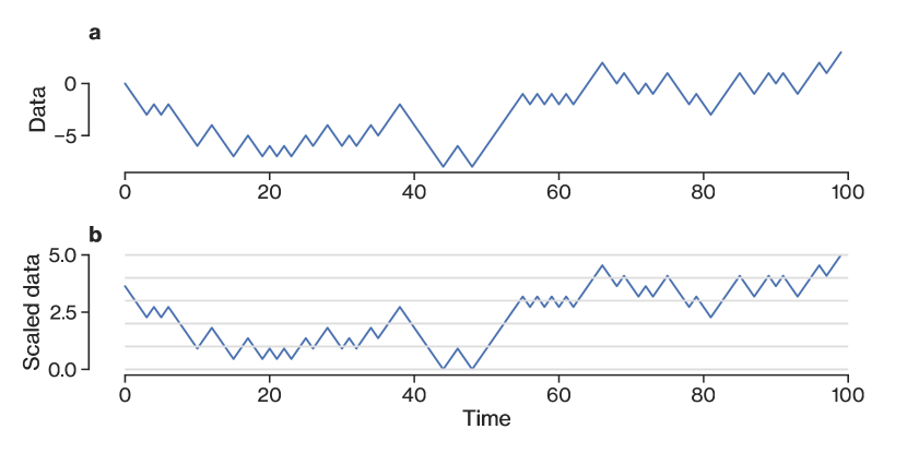
Figure 1: Original data and rounded data. (a) The original data series. (b) The corresponding rounded data series, shifted to fit within evenly spaced intervals according to the number of stripes chosen, with grid lines drawn at stripe boundaries.

Once the data has been rounded to the stripe widths, events are recorded at all times when the data crosses, or intersects, a stripe. To determine whether a crossing occurs at time $t$, MDEA checks two conditions:

$$X_{t}\stackrel{{\scriptstyle?}}{{<}}\mathrm{floor}(X_{t-1}+1),$$ (4)

$$X_{t}\stackrel{{\scriptstyle?}}{{>}}\mathrm{ceil}(X_{t-1}-1).$$ (5)

If either of these conditions is false then a crossing must have occurred at time $t$. If a crossing occurs at time $t$ a 1 is appended to the event array, $E$, at index $t$; if not a 0 is appended. This process is shown in Figure 2.

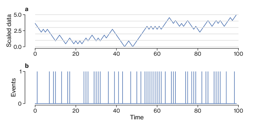
Figure 2: Rounded data and events. (a) The rounded data. (b) Events being recorded at every time index in the rounded data where either Equation 4 or Equation 5 are false. All events have magnitude 1 and are positive (Grigolini et al., 2001).

The next step is to construct a diffusion trajectory, $Y$, from the recorded events. This is done by taking the cumulative sum of the event array, $E$:

$$Y_{n}=\sum_{t=0}^{n}E_{t},$$ (6)

where $n$ starts off at the first index of the array—0 in most programming languages—then increases by 1 until $n$ equals the length of the array. This is depicted in Figure 3.

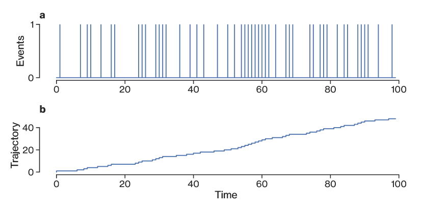
Figure 3: Events and diffusion trajectory. (a) Event array. (b) Diffusion trajectory constructed by taking cumulative sum of the events array.

DEA uses a moving window to examine this diffusion trajectory. The process is similar to some other time-series analysis methods which use moving windows. In particular, the moving window is used similarly to Detrended Fluctuation Analysis (DFA) (Peng et al., 1994). The difference is that DFA uses windows that do not overlap, while DEA uses window positions advancing one time index by one with much overlap. This similarity and the rationale behind this decision is discussed in Grigolini et al. (2001). For this demonstration only one window length, $l=100$, is defined, which is placed at fixed positions (end to end) on the diffusion trajectory. This makes the windows and snapshots easier to visualize. In practice a set of window lengths is defined and each stepped down the trajectory, shifting one index at a time. For this demonstration only one possible window length is used and only a subset of the window positions.

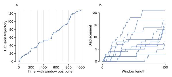
Figure 4: Moving window and trajectory slices. (a) The diffusion trajectory with grid lines drawn at a set of window positions, using $l=100$. (b) The slices of the diffusion trajectory across each of the window positions in (a), laid atop each other and shifted to start from the same origin along the $y$-axis. Here the first 1000 steps in the series are used.

Once these trajectory slices have been computed the next step is to make a histogram of their displacements. For each window length $l$, stepping the window along the trajectory generates many slices, each of which goes some distance from the origin – along the y-axis in Figure 4. These displacements are binned in a histogram, which is then normalized to turn it into a probability distribution, $P(l)$. One such histogram is plotted in Figure 5.

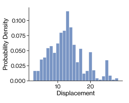
Figure 5: Distribution of diffusion slices. Histogram of the displacements of diffusion trajectory slices; normalized to form a probability distribution, $P(l)$.

Information entropy, or Shannon entropy (Shannon, 1948), is defined:

$$S(Y)=-\sum_{i}P(y_{i})\log(P(y_{i})),$$ (7)

where $S$ is the entropy, $Y$ the random variable, $y_{i}$ the possible values of $Y$, and $P(y_{i})$ the probabilities associated with each value. For DEA, with $Y$ being the value of the diffusion trajectory at $t=l$ and with probability distributions $P_{l}$ corresponding to window length $l$, this goes:

$$S_{l}(Y)=-\sum_{i}P_{l}(y_{i})\ln(P_{l}(y_{i})).$$ (8)

DEA uses many window lengths, constructs probability distributions for each, and calculates the entropy corresponding to each according to Equation 8. Figure 6 illustrates an example of the result.

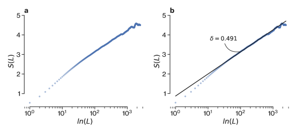
Figure 6: Principal result of MDEA. (a) Shannon entropy $S(l)$ vs. natural log of window lengths $\ln(l)$. The choice of natural log of $l$ for axis scale reveals any extant power-law behavior. (b) The slope of the linear fit, $\delta$, is the scaling of the time-series process. For a random walk such as this data, $\delta=0.5$ is the expected value for MDEA to measure.

The goal of DEA is to extract the scaling of the data series. This is done by using the relation between $S$ and $l$:

$$S(l)=\delta\ln(l)+C,$$ (9)

where $\delta$ is the scaling of the process and $C$ is some constant (Scafetta and Grigolini, 2002). This relation is linear, in log-scale. Therefore, if a linear fit is performed in log-scale, as is shown in Figure 6, the slope is the scaling, $\delta$, of the time-series.

Clauset et al. (2009) show that using least-squares to fit the slope for a line of the form in equation 9 introduces systematic errors. MDEA therefore includes support for using more robust linear fitting: the Siegel (1982) and Theil (1950)-Sen (1968) methods. These methods fit an ensemble of lines between pairs of data points and use the median slope of the ensemble as the slope of the fit line. This makes them much more robust against outliers, and avoids the systematic errors introduced by least-squares.

Discussion

MDEA measures a kind of temporal complexity related to criticality. The scaling, $\delta$, that MDEA outputs provides a measure of the complexity present in the data set. The behavior of $\delta$ and its relation to criticality and complexity parameters is discussed in depth in Grigolini et al. (2001) and Scafetta and Grigolini (2002). For this tutorial it suffices to understand the basic rules for interpreting the results. For a completely non-complex process, such as a random walk, MDEA yields $\delta=0.5$. For a process at criticality, MDEA yields $\delta=1$. Therefore, $\delta$ represents a measure of the complexity present in the process: the closer $\delta$ is to 1 the closer the process is to criticality.

MDEA offers significant advantages over the original DEA. In DEA the original time-series is used as the diffusion trajectory with no pre-processing. As a result several kinds of noise are able to affect the measured scaling. For example, if the time-series is characterized by fractional Brownian motion (FBM) (Mandelbrot and Ness, 1968), DEA will measure a scaling equal to the Hurst index of the FBM. Even in cases where FBM is only a component of the data and not a complete characterization, the scaling measured by DEA is significantly affected by the FBM contribution. MDEA filters out any existing FBM contribution to the scaling, allowing examination and quantification of other complexity sources in the data (Culbreth et al., 2019).

In particular, MDEA improves detection of events that occur at time intervals distributed according to a power law. These events appear in several complex processes, and they are conjectured to be a signature of a complex system undergoing self-organization in time (Bohara et al., 2018).

Future Development

MDEA development is ongoing and several key areas remain where MDEA requires improvement. Most urgent of these is the determination of fitting interval. So far this interval has been chosen on a case-by-case basis by the researcher looking at the plot of $S(l)$ vs. $\ln(l)$ and adjusting the fit to lie along the linear portion. This is not rigorous and quite unsatisfactory. Using the Siegel (1982) and Theil (1950)-Sen (1968) robust linear fitting methods removes the need to set a lower bound for this fitting interval, but still require an upper bound. A rigorous and standardized method of determining the correct fitting interval is urgently needed, perhaps by performing iterated fits and adjusting the fit interval based on the residuals. Alternatively, since equation 9 has a power law form, it may be possible to use maximum likelihood estimation to obtain the scaling (Clauset et al., 2009). Using maximum likelihood estimation would remove the need to set a fit interval at all.

Secondly, the method for determining how many stripes ought to be used requires improvement. So far this is another case-by-case choice on the part of the researcher, usually done by testing several possible values and trying to guess which one is best. The best guidance thus far developed is that the correct number of stripes is usually between 2 and 70. However, there is currently no rigorous method for determining the correct number, or even for judging whether the researcher’s guess is good or bad. Further work is urgently needed to develop a rigorous method for determining how many stripes ought to be used, which should follow the direction established by Allegrini et al. (2002).

Finally, the MDEA code requires further optimization, especially for run-time speed. The MDEA code hosted on GitHub is written in Python and uses NumPy (Harris et al., 2020), which supports using Fortran code modules to speed up computations. Future development should investigate whether this functionality can be implemented into MDEA, or should develop a bespoke integration using modules written in other high-performance languages, such as Rust. Development in this direction would provide substantial runtime improvements.

References

- Allegrini et al. (2002) Allegrini, P., Balocchi, R., Chillemi, S., Grigolini, P., Hamilton, P., Maestri, R., Palatella, L., Raffaelli, G., 2002. Real event detection and the treatment of congestive heart failure: an efficient technique to help cardiologists to make crucial decisions. arXiv preprint cond-mat/0209038 .
- Bohara et al. (2017) Bohara, G., Lambert, D., West, B.J., Grigolini, P., 2017. Crucial events, randomness, and multifractality in heartbeats. Physical Review E 96, 062216.
- Bohara et al. (2018) Bohara, G., West, B.J., Grigolini, P., 2018. Bridging waves and crucial events in the dynamics of the brain. Frontiers in physiology 9, 1174.
- Cai et al. (2006) Cai, S.M., Zhou, P.L., Yang, H.J., Yang, C.X., Wang, B.H., Zhou, T., 2006. Diffusion entropy analysis on the scaling behavior of financial markets. Physica A: Statistical Mechanics and its Applications 367, 337–344.
- Clauset et al. (2009) Clauset, A., Shalizi, C.R., Newman, M.E., 2009. Power-law distributions in empirical data. SIAM review 51, 661–703.
- Culbreth et al. (2019) Culbreth, G., West, B., Grigolini, P., 2019. Entropic approach to the detection of crucial events. Entropy 21, 178. URL: https://doi.org/10.3390/e21020178, doi:10.3390/e21020178.
- Grigolini et al. (2001) Grigolini, P., Palatella, L., Raffelli, G., 2001. Asymmetric anomalous diffusion: an efficient way to detect memory in time series. Fractals 09, 439–449. URL: https://doi.org/10.1142/s0218348x01000865, doi:10.1142/s0218348x01000865.
- Harris et al. (2020) Harris, C.R., Millman, K.J., van der Walt, S.J., Gommers, R., Virtanen, P., Cournapeau, D., Wieser, E., Taylor, J., Berg, S., Smith, N.J., et al., 2020. Array programming with numpy. Nature 585, 357–362.
- Jelinek et al. (2020) Jelinek, H.F., Tuladhar, R., Culbreth, G., Bohara, G., Cornforth, D., West, B.J., Grigolini, P., 2020. Diffusion entropy vs. multiscale and rényi entropy to detect progression of autonomic neuropathy. Frontiers in Physiology 11.
- Mandelbrot and Ness (1968) Mandelbrot, B.B., Ness, J.W.V., 1968. Fractional brownian motions, fractional noises and applications. SIAM Review 10, 422–437. URL: https://doi.org/10.1137/1010093, doi:10.1137/1010093.
- Mega et al. (2003) Mega, M.S., Allegrini, P., Grigolini, P., Latora, V., Palatella, L., Rapisarda, A., Vinciguerra, S., 2003. Power-law time distribution of large earthquakes. Physical Review Letters 90, 188501.
- Peng et al. (1994) Peng, C.K., Buldyrev, S.V., Havlin, S., Simons, M., Stanley, H.E., Goldberger, A.L., 1994. Mosaic organization of dna nucleotides. Physical review e 49, 1685.
- Scafetta and Grigolini (2002) Scafetta, N., Grigolini, P., 2002. Scaling detection in time series: Diffusion entropy analysis. Phys. Rev. E 66, 036130. URL: https://link.aps.org/doi/10.1103/PhysRevE.66.036130, doi:10.1103/PhysRevE.66.036130.
- Sen (1968) Sen, P.K., 1968. Estimates of the regression coefficient based on kendall’s tau. Journal of the American statistical association 63, 1379–1389.
- Shannon (1948) Shannon, C.E., 1948. A mathematical theory of communication. Bell System Technical Journal 27, 379–423. URL: https://doi.org/10.1002/j.1538-7305.1948.tb01338.x, doi:10.1002/j.1538-7305.1948.tb01338.x.
- Siegel (1982) Siegel, A.F., 1982. Robust regression using repeated medians. Biometrika 69, 242–244.
- Theil (1950) Theil, H., 1950. A rank-invariant method of linear and polynomial regression analysis. Indagationes mathematicae 12, 173.
- Tuladhar et al. (2018) Tuladhar, R., Bohara, G., Grigolini, P., West, B.J., 2018. Meditation-induced coherence and crucial events. Frontiers in physiology 9, 626.