Two-step BEC coming from a temperature dependent energy gap

Abstract

We report the effects on the thermodynamic properties of a 3D Bose gas caused by a temperature dependent energy gap $\Delta(T)$ at the lower edge of the energy spectrum of the particles constituting the Bose gas which behaves like an ideal Bose gas when the gap is removed. Explicit formulae are given for the critical temperature, the condensate fraction, the internal energy and the isochoric specific heat, which are calculated for three different gaps that abruptly go to zero at temperature $T_{B}$, as well as for the damped counterparts whose drop to zero we have smoothed. In particular, for the undamped BCS (Bardeen, Cooper and Schrieffer) gap it is observed that the Bose-Einstein condensation (BEC) critical temperature $T_{c}$ is equal to that of the ideal Bose gas $T_{0}$, for all $T_{B}\leq T_{0}$; surprisingly, the condensate fraction presents two different filling rates of the ground state at $T_{c}=T_{0}$ and at $T_{B}<T_{0}$; while the specific heat shows a finite jump at $T_{c}$ as well as a divergence at $T_{B}$. Three-dimensional infinite Bose gas results are recovered when the temperature independent gap is either a constant or equal to zero.

I Introduction

Bose-Einstein condensation (BEC) is a physical phenomenon which has permeated many areas of physics, from condensed matter to cosmology Das . In particular, some superconductivity theories Lee ; Tolmachev consider Cooper pairs as composite bosons, an assumption that becomes more precise the smaller the correlation length of the pairs is, like in cuprates. It is well known from BCS theory that Cooper pairs have a temperature-dependent energy gap between their ground and their first excited state energy, which promotes superconductivity. This gap begins with a value at $T=0$ which decreases as the temperature increases, becoming zero at the superconducting critical temperature. On the other hand, some properties of superfluid helium four, such as its temperature dependent specific heat exponential behavior near $T=0$ was explained by London London , suggesting that helium superfluidity is motivated by a BEC of the helium atoms with an artificial constant gap in their energy dispersion relation London2 ; japoneses . Although the exponential behavior of the isochoric specific heat is reproduced for low temperatures, the BE critical temperature ($T_{c}$) increases beyond the BE critical temperature of an ideal Bose gas of helium atoms as the energy gap magnitude increases. This behavior is contrary to what is observed in helium, where the interaction among atoms reduces the superfluidity critical temperature below the 3D BEC critical temperature of an ideal Bose gas (IBG) when its particle mass and density are that of liquid helium four. Although many theoretical efforts gapjustification have been made to justify the gap as a result of interactions among the bosons, the gap not only has not showed up but there are arguments against its existence HP . It is worth mentioning that even though the critical temperature for a IBG plus a constant gap like that proposed by London, has a BEC critical temperature which encreases proportionally to the gap magnitude. However, when the gap decreases to zero as the temperature increases, we analize two possibilities: a) if the temperature $T_{B}$ at which the gap becomes zero, is less than or equal to $T_{0}$ (IBG critical temperature), the BEC critical temperature $T_{c}$ is equal to $T_{0}$, and otherwise, b) if $T_{B}>T_{0}$ the temperature $T_{c}$ is greater than $T_{0}$ and depends on $T_{B}$ as well as on the gap shape.

In this work we discuss the effects on the thermodynamic properties of a 3D Bose gas caused by a temperature dependent gap $\Delta(T)$ in the energy spectrum of the particles constituting the gas which behaves like an IBG without the gap. Although this problem seems to be an academic problem, there are evidences of Bose gases with this type of dispertion relation like those emanating from imperfections in the networks where the bosons are found juan .

In Sec. II after defining our system, we calculate: a) the critical temperature as a function of gap; b) the condensate fraction and the temperature derivative of the condensate fraction multiplied by temperature and divided by the condensate fraction. In Sec. III we give the following thermodynamic properties: the chemical potential, the internal energy, the isochoric specific heat as functions of temperature and the jump height of the specific heat at $T_{c}$. In Sec. IV we apply the results of Sections II and III to three types of undamped and damped gaps but emphasizing the properties of the Bose gas with a BCS gap. In Sec. V we give our conclusions.

II 3D Bose gas with quadratic dispersion relation plus a temperature dependent gap

Our system is a 3D infinite Bose gas of $N$ particles of mass $m$ whose dispersion relation energy as a function of its momentum magnitude $\hbar k$ is given by

$$\varepsilon_{k}=\left\{\begin{array}[]{c}\varepsilon_{0}{\ \ \ \ \ \ \ \ \quad\ \quad\ \qquad\ \ \ \ \ \ \mbox{if}\ \ \ }k=0\\ \varepsilon_{0}+\Delta(T)+\hbar^{2}k^{2}/2m{\ \ \ \mbox{if}\ \ \ }k>0\end{array}\right.,$$ (1)

where $\Delta(T)$ is the energy gap between the ground state energy $\varepsilon_{0}$ and the first excited state energy $\varepsilon_{0}+\Delta(T)$. From here on we writte $\Delta_{0}\equiv\Delta(T=0)$ and $\Delta\equiv\Delta(T)$.

II.1 BEC critical temperature

For a finite temperature the particle number $N$ is distributed between the energy ground state and the excited states, i.e., $N=N_{0}(T)+N_{e}(T)$ with

$$N_{0}(T)={\frac{1}{e^{\beta[\mathbf{\varepsilon}_{0}-\mu(T)]}-1}}$$ (2)

the particles in the energy ground state and

$$N_{e}=\sum_{\mathbf{k\neq 0}}n_{k}=\sum_{\mathbf{k\neq 0}}{\frac{1}{e^{\beta[\mathbf{\varepsilon}_{k}-\mu(T)]}-1}}$$ (3)

the particles in the excited states, with $\beta\equiv 1/k_{B}T$, and $\mu(T)\leq\varepsilon_{0}$ the chemical potential.

In order to write the expression of $N_{e}$ in the thermodynamic limit, we convert the sum (3) into the integral

$$N_{e}=\frac{1}{(2\pi/L)^{3}}\int_{\mathbf{k\neq 0}}^{\infty}{\frac{4\pi k^{2}dk}{e^{\beta(\varepsilon_{k}-\mu(T))}-1}},$$ (4)

where $\varepsilon_{k}=\varepsilon_{0}+\Delta(T)+\hbar^{2}k^{2}/2m$. Defining $\xi\equiv\beta\hbar^{2}k^{2}/2m$, Eq. (4) becomes

$$N_{e} = \frac{L^{3}(2m/\hbar^{2})^{3/2}}{4\pi^{2}\beta^{3/2}}\int_{0}^{\infty}{\frac{\xi^{1/2}d\xi}{e^{-\beta(\mu-\varepsilon_{0}-\Delta)}\ e^{\xi}-1}}$$ (5)

$${=} \frac{L^{3}(2m/\hbar^{2})^{3/2}}{4\pi^{2}\beta^{3/2}}g_{3/2}(z_{1})\Gamma(3/2)$$

with $z_{1}\equiv\exp[\beta(\mu-\varepsilon_{0}-\Delta)]\leq 1$ and $g_{3/2}(z_{1})$ is the Bose function of order 3/2.

The Bose Einstein critical temperature $T_{c}$ is the smaller temperature for which $N_{0}(T_{c})/N\simeq 0$ and $N_{e}/N\simeq 1$, so as a consequence $\mu(T)=\varepsilon_{0}$ for $T\leq T_{c}$. Therefore at $T_{c}$

$$N=\frac{L^{3}(2m/\hbar^{2})^{3/2}}{4\pi^{2}\beta_{c}^{3/2}}g_{3/2}(z_{1c})\Gamma(3/2)$$ (6)

with $z_{1c}\equiv\exp[-\beta_{c}\Delta(T_{c})]\leq 1.$ For $\Delta_{0}=0$, $z_{1c}=1$ and we recover the critical temperature $T_{0}$ of an IBG via the relation

$$N=\frac{L^{3}(2m/\hbar^{2})^{3/2}}{4\pi^{2}\beta_{0}^{3/2}}\zeta(3/2)\Gamma(3/2),$$ (7)

with $\beta_{0}=1/k_{B}T_{0}$ and $T_{0}$ the BEC critical temperature for an IBG with a number density equal to that of our system. Note that in this case the dispersion relation for the Bose gas starts at $\varepsilon_{0}$ but has no effect on the critical temperature as this is a translation of the starting point of the particle energies.

For $\Delta_{0}\neq 0$, from the ratio between (6) and (7),

$$1 = \frac{\beta_{0}^{3/2}g_{3/2}(z_{1c})}{\beta_{c}^{3/2}\zeta(3/2)}\qquad$$

$${\mbox{and}\qquad}T_{c} = \left(\frac{\zeta(3/2)}{g_{3/2}(z_{1c})}\right)^{2/3}T_{0}$$ (8)

Since $z_{1c}\leq 1$, $g_{3/2}(z_{1c})\leq\zeta(3/2)$ therefore $T_{c}\geq T_{0}$.

II.2 Condensate fraction

For $T<T_{c}$ the number of particles in the ground state $N_{0}(T)$ is comparable with the total number of particles $N$ and the condensate fraction $N_{0}(T)/N$ is

$$\frac{N_{0}(T)}{N}=1-\frac{N_{e}}{N}.$$ (9)

Sustituting (5) and (6) in the last equation we obtain

$$\frac{N_{0}(T)}{N}=1-\frac{T^{3/2}g_{3/2}(z_{1<})}{T_{c}^{3/2}g_{3/2}(z_{1c})}\xrightarrow[\Delta\to 0]{}1-(T/T_{0})^{3/2},$$ (10)

with $z_{1<}\equiv Exp[-\beta\Delta]$. When $T\leq T_{c}$, $z_{1}=z_{1<}$ and $z_{1c}=z_{1}(T_{c})$. For $\Delta(T)=0$ we recover the condensate fraction for an IBG.

Now to analyze how quickly the ground state is populated, we calculate the coefficient $(T/N_{0})dN_{0}(T)/dT$. For $T\leq T_{c}$ we derive $N_{0}$ given in Eq. (10) with respect to the temperature

$$\begin{split}\frac{dN_{0}(T)}{dT}&=-\frac{NT^{1/2}}{T_{c}^{3/2}g_{3/2}(z_{1c})}\times\\ &\left[\frac{3}{2}g_{3/2}(z_{1<})+g_{1/2}(z_{1<})\left(\frac{\Delta}{k_{B}T}-\frac{1}{k_{B}}\frac{d\Delta}{dT}\right)\right]\end{split}$$

and multiplying it by $T/N_{0}$, we obtain

$$\frac{T}{N_{0}}\frac{dN_{0}(T)}{dT}=\frac{\frac{3}{2}g_{3/2}(z_{1<})+g_{1/2}(z_{1<})\left(\frac{\Delta}{k_{B}T}-\frac{1}{k_{B}}\frac{d\Delta}{dT}\right)}{g_{3/2}(z_{1<})-\left(\frac{T_{c}}{T}\right)^{3/2}g_{3/2}(z_{1c})}.$$ (11)

For $T>T_{c}$ we derive Eq. (2)

$$\frac{dN_{0}}{dT}=\frac{e^{\beta[\varepsilon_{0}-\mu(T)]}}{\left[e^{\beta[\varepsilon_{0}-\mu(T)]}-1\right]^{2}}\beta\left[\frac{\varepsilon_{0}-\mu(T)}{T^{2}}+\frac{d\mu(T)}{dT}\right]$$ (12)

which is multiplied by the coefficient $T/N_{0}$ to obtain

$$\frac{T}{N_{0}}\frac{dN_{0}(T)}{dT}=\frac{\frac{\Delta}{k_{B}T}+\frac{3}{2}\frac{g_{3/2}(\exp[\beta(\mu-\varepsilon_{0}-\Delta)])}{g_{1/2}(\exp[\beta(\mu-\varepsilon_{0}-\Delta)])}}{e^{\beta(\mu-\varepsilon_{0})}-1}.$$ (13)

The expression for the derivative of the chemical potential Eq. (16) is given in the next section.

III Thermodynamic properties

III.1 Chemical potential

All the thermodynamic properties of our system are chemical potential dependent.

For $T>T_{c}$ all bosons are in the excited states, i.e., $N=N_{e}$. Equating equations (5) and (7), and after canceling some factors, we obtain

$$\frac{g_{3/2}(z_{1})}{\beta^{3/2}}=\frac{\zeta(3/2)}{\beta_{0}^{3/2}}.$$ (14)

Remembering that $z_{1}=\exp[\beta(\mu-\varepsilon_{0}-\Delta)]$, the last equation can be rewritten as

$$(T/T_{0})^{3/2}g_{3/2}(\exp[\beta(\mu-\varepsilon_{0}-\Delta)])=\zeta(3/2).$$ (15)

This is an implicit equation for the chemical potential as a function of temperature, valid only for $T\geq T_{c}$, since for $T\leq T_{c}$ $\mu=\varepsilon_{0}$.

To calculate the specific heat we need the temperature derivative of the chemical potential, which we obtain differentiating the expression (15)

$$\begin{split}\frac{1}{k_{B}}\frac{d\mu}{dT}=&\frac{1}{k_{B}}\frac{d\Delta}{dT}+\frac{\mu-\mathbf{\varepsilon}_{0}-\Delta}{k_{B}T}\\ &-\frac{3}{2}\frac{g_{3/2}(\exp[\beta(\mu-\varepsilon_{0}-\Delta)])}{g_{1/2}(\exp[\beta(\mu-\varepsilon_{0}-\Delta)])}.\end{split}$$ (16)

III.2 Internal energy

The internal energy $U(L^{d},T)$ is given by the sum of the energies of the particles both in the ground and in the excited states, such that using Eqs. (2) and (3) we get

$$U(L^{d},T)={\frac{\varepsilon_{0}}{e^{\beta[\mathbf{\varepsilon}_{0}-\mu(T)]}-1}}+\sum_{\mathbf{k\neq 0}}{\frac{\varepsilon_{k}}{e^{\beta[\mathbf{\varepsilon}_{k}-\mu(T)]}-1}}\ .$$ (17)

In the thermodynamic limit, using the energy espectrum Eq. (1), we obtain

$$\begin{split}&U(L^{d},T)={\frac{\varepsilon_{0}}{e^{\beta[\varepsilon_{0}-\mu(T)]}-1}}\\ &+\frac{L^{3}4\pi}{(2\pi)^{3}}\int_{0^{+}}^{\infty}\frac{(\varepsilon_{0}+\Delta+\hbar^{2}k^{2}/2m)k^{2}dk}{e^{\beta{[\varepsilon_{0}+\Delta+\hbar^{2}k^{2}/2m-\mu(T)]}}-1}.\end{split}$$ (18)

Defining $\xi\equiv\beta[\hbar^{2}k^{2}/2m]$, $d\xi=(\beta\hbar^{2}/2m)2kdk$ and $\xi^{3/2}=(\beta\hbar^{2}/2m)^{3/2}k^{3}$, last equation becomes

$$\begin{split}U(L^{d},T)&=\mathbf{\varepsilon}_{0}N_{0}+\\ &(\mathbf{\varepsilon}_{0}+\Delta)\frac{L^{3}(2m/\hbar^{2})^{3/2}}{4\pi^{2}\beta^{3/2}}\int_{0}^{\infty}{\frac{\xi^{1/2}d\xi}{z^{-1}\ e^{\xi}-1}}\\ &+\frac{L^{3}}{4\pi^{2}}\frac{(2m/\hbar^{2})^{3/2}}{\beta^{5/2}}\int_{0^{+}}^{\infty}\frac{\xi^{3/2}d\xi}{z_{1}^{-1}e^{\xi}-1}.\end{split}$$ (19)

In the right hand side of the last equation, the second term is the number of excited particles times ($\mathbf{\varepsilon}_{0}+\Delta$) (see Eq. (5)). Then, we rewrite the internal energy as

$$\begin{split}U(L^{d},T)&=\mathbf{\varepsilon}_{0}N+\Delta N_{e}\\ &+\frac{L^{3}}{4\pi^{2}}\frac{(2m/\hbar^{2})^{3/2}}{\beta^{5/2}}\Gamma(5/2)g_{5/2}(z_{1}),\end{split}$$ (20)

where we have replaced the last integral of (19) by its value $\Gamma(5/2)g_{5/2}(z_{1})$ (see Appendix D Pathria ). Dividing it by $Nk_{B}T$, and taking the values of $N_{e}$ and $N$ given in Eqs. (5) and (6) respectively, equation (20) becomes

$$\begin{split}&\frac{U(L^{d},T)}{Nk_{B}T}=\frac{\mathbf{\varepsilon}_{0}}{k_{B}T}\\ &+\left[\frac{\Delta(T)}{k_{B}T}\frac{g_{3/2}(z_{1})}{g_{3/2}(z_{1c})}+\frac{3}{2}\frac{g_{5/2}(z_{1})}{g_{3/2}(z_{1c})}\right]\left(\frac{T}{T_{c}}\right)^{3/2}.\end{split}$$ (21)

III.3 Specific heat

The isochoric specific heat comes from deriving the internal energy (21) with respect to the temperature. For $T\leq T_{c}$ we obtain

$$\frac{C_{V}}{Nk_{B}}=\left[\left(\frac{\Delta^{2}}{(k_{B}T)^{2}}-\frac{\Delta}{k_{B}^{2}T}\frac{d\Delta}{dT}\right)g_{1/2}(z_{1<})+\frac{15}{4}g_{5/2}(z_{1<})\right.$$

$$+\left.\left(3\frac{\Delta}{k_{B}T}-\frac{1}{2k_{B}}\frac{d\Delta}{dT}\right)g_{3/2}(z_{1<})\right]\frac{\left(T/T_{c}\right)^{3/2}}{g_{3/2}(z_{1c})}.$$ (22)

For $T\rightarrow 0$, $z_{1<}\rightarrow 0$, and using the approximation $g_{\sigma}(z_{1<})\approx z_{1<}$ valid for $\sigma=5/2,3/2$ and $1/2$, the last Ec. (22) reduces to

$$\frac{C_{V}}{Nk_{B}}=\left[\frac{\Delta^{2}}{(k_{B}T)^{2}}-\frac{\Delta}{k_{B}^{2}T}\frac{d\Delta}{dT}+\frac{3\Delta}{k_{B}T}-\frac{1}{2k_{B}}\frac{d\Delta}{dT}+\frac{15}{4}\right]$$

$$\times\frac{\mbox{Exp}[-\Delta/k_{B}T]\left(T/T_{c}\right)^{3/2}}{g_{3/2}(z_{1c})}$$ (23)

where we notice that for small temperatures the specific heat has an exponential behavior when we introduce a gap in the dispersion relation. In fact, for a constant gap $\Delta_{0}$,

$$\begin{split}\frac{C_{V}}{Nk_{B}}=\left[\frac{\Delta_{0}^{2}}{(k_{B}T)^{2}}+\frac{3\Delta_{0}}{k_{B}T}+\frac{15}{4}\right]\frac{\exp[-\Delta_{0}/k_{B}T]\left(T/T_{c}\right)^{3/2}}{g_{3/2}(z_{1c})}\end{split}$$ (24)

which decays exponentially as given by expression (28) of Ref. Martinez-Herrera with $s=2$ and $d=3$, and experimentally observed in helium four near absolute zero temperature.

When $\Delta(T)\to 0$ Eq. (23) reduces to

$$\begin{split}\frac{C_{V}}{Nk_{B}}=\frac{15}{4}\frac{\left(T/T_{c}\right)^{3/2}}{\zeta(3/2)}\end{split}$$ (25)

that is, $C_{V}$ is proportional to $T^{3/2}$ as expected for a 3D IBG.

To obtain the specific heat for $T>T_{c}$ we derive the internal energy Eq. (21) from where we obtain

$$\begin{split}\frac{C_{V}}{Nk_{B}}=\frac{d}{dT}\left(\frac{U}{Nk_{B}}\right)=\frac{15}{4}\frac{g_{5/2}(z_{1})}{g_{3/2}(z_{1c})}\left(\frac{T}{T_{c}}\right)^{3/2}\\ +\left[\frac{d\Delta(T)}{k_{B}dT}-\frac{9}{4}\frac{g_{3/2}(z_{1})}{g_{1/2}(z_{1})}\right]\frac{g_{3/2}(z_{1})}{g_{3/2}(z_{1c})}\left(\frac{T}{T_{c}}\right)^{3/2}\end{split}$$ (26)

Note that for all temperature regimes, the specific heat is $\mathbf{\varepsilon}_{0}$ independent.

On the other hand, since we have different expressions for the specific heat below and above $T_{c}$, we expect that for certain cases we obtain two different values for $C_{V}$ at the transition temperature. Let $C_{V}(T^{-}_{c})$ be the specific heat from (22) evaluated at $T_{c}$ and $C_{V}(T^{+}_{c})$ the value obtained by evaluating (26) at $T_{c}$. Thus, the specific heat discontinuity at $T_{c}$ is given by

$$\begin{split}\frac{C_{V}(T^{-}_{c})-C_{V}(T^{+}_{c})}{Nk_{B}}=\left[\frac{\Delta^{2}}{(k_{B}T)^{2}}-\frac{\Delta}{k_{B}^{2}T}\frac{d\Delta}{dT}\right]_{T_{c}}\frac{g_{1/2}(z_{1c})}{g_{3/2}(z_{1c})}\\ +\left[\frac{3\Delta}{k_{B}T_{c}}-\frac{3}{2k_{B}}\frac{d\Delta}{dT}\right]_{T_{c}}+\frac{9}{4}\frac{g_{3/2}(z_{1c})}{g_{1/2}(z_{1c})}\end{split}$$ (27)

when $\Delta=0$ we recover Eq. (14) of Aguilera-Navarro for the case $d=3$ and $s=2$.

Figure 1: Examples of temperature dependent gaps. For these cases $\Delta_{0}=k_{B}T_{0}$ and $T_{B}=1.5T_{0}$.

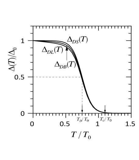
Figure 2: The same gaps of Fig. 1 but now the undamped gaps are multiplied by the damping function $f(T)=1/(\exp[b(T/T_{D}-1)]+1)$. For these cases $\Delta_{0}=k_{B}T_{0}$, $T_{B}=10\,T_{0}$, $b=10$, $T_{D}=0.75\,T_{0}$. In particular for $\Delta_{DB}$ the resulting $T_{c}=1.09\,T_{0}$.

IV Applications

IV.1 Gap Types

Here we calculate some thermodynamic properties with the expressions given above for a Bose gas whose particles have an energy spectrum with one of six different temperature-dependent gaps. We begin by analyzing three gaps which decrese with temperature, becoming zero above the temperature $T_{B}$, i.e.,

$$\Delta(T)=\left\{\begin{array}[]{c}g(T)\ \ \ \ \ \ \ \ {\quad\mbox{if}\ \ \ }T<T_{B}\\ \quad 0\quad\quad{\ \,\,\,\quad\ \ \mbox{if}\ \ \ }T\geq T_{B}\end{array}\right.$$ (28)

where $g(T)=\Delta_{0}(1-T/T_{B})^{1/2}$ (BCS gap), $g(T)=\Delta_{0}(1-T/T_{B})$ (Linear gap) or $g(T)=\Delta_{0}$ (Step gap). In Fig. 1 we show these three gaps for $T_{B}=1.5T_{0}$ and $\Delta_{0}=k_{B}T_{0}$.

Although the BCS Theory suggests an abrupt creation of many Cooper pairs at and below the superconducting critical temperature, it is expected seudogap that at a higher pseudo-gap temperature pairs will begin to form, increasing in number as the system cools until it reaches a critical density to develop superconductivity. To explore the effect of Cooper pairs creation above the superconducting critical temperature on the gap shape, we explore multiplying the BCS gap, as well as the other two gap functions, by the damping function $f(T)=1/(\exp[b(T/T_{D}-1)]+1)$, where $T_{D}$ is a damping temperature whose magnitude indicates the temperature for wich $f(T_{D})=1/2$, and $b$ a large number to assure that when $T<<T_{D}$ we recover the undamped gap function $g(T)$. Then, the expressions for the three damped gaps are

$$\Delta_{\alpha}(T)=\frac{g(T)}{\exp[b(T/T_{D}-1)]+1}$$ (29)

where $\alpha=DB,DL$ and $DS$, which mean damped BCS gap, damped Linear gap and damped Step gap, respectively. These damped gaps are plotted in Fig. 2 where, unlike Fig. 1, gaps have a smooth decay close to $T_{0}$ showing finite values of their derivatives, and going smoothly to zero at $T_{B}$. The parameters for the three damped gaps in Fig. 2 are $\Delta_{0}=k_{B}T_{0}$, $T_{B}=10\,T_{0}$, $b=10$, $T_{D}=0.75\,T_{0}$. For this $T_{D}$ the Bose gas with the gap $\Delta_{DB}$ has a critical temperature $T_{c}=1.09\,T_{0}$ where the gap is different from zero but very small since its value is $0.0088\ \Delta_{0}$. A similar smooth gap decay near $T_{c}$ is reported in Ref. Dougherty for gaps of Nb, Ta, Pb, Hg, Sn, In, Al, Ga, Zn and Cd obtained from a thermodynamic analysis of experimental data.

IV.2 Gap effect on the BEC critical temperature

Figure 3: Bose-Einstein critical temperature $T_{c}/T_{0}$ as function of $T_{B}/T_{0}$ for the three undamped gaps. Dashed line is $T_{c}=T_{B}$.

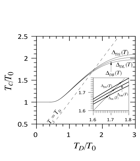
Figure 4: Bose-Einstein critical temperature $T_{c}/T_{0}$ as a function of the damping temperature $T_{D}/T_{0}$ using the tree damped gaps of Eq. (29), where $\Delta_{0}=k_{B}T_{0}$, $T_{B}=10\,T_{0}$, and $b=10$. Dashed line is $T_{c}=T_{D}$. In the inset we show the $T_{D}$ temperatures for which $T_{D}=T_{C}$.

In Fig. 3 we show the critical temperatures as functions of $T_{B}/T_{0}$ using the undamped gaps described by Eq. (28) for the three forms of $g(T)$ (the BCS, the Linear and the Step gap). For all three gaps, regardless of their shapes, we find that when $T_{B}\leq T_{0}$ the BEC critical temperature $T_{c}=T_{0}$. When $T_{B}>T_{0}$ the BEC critical temperature $T_{c}>T_{0}$ and gap shape dependent, except when $T_{B}>>T_{0}$, where the critical temperatures approach that for a constant gap $\Delta_{0}$ for every temperature.

We note that for the three gaps their temperature derivatives at $T_{B}$ have a jump, which becomes infinite for the BCS gap. In order to avoid a sudden drop to zero of the gap, which causes infinities in the thermodynamic properties, we multiply the undamped gaps by a damping function $f(T)$ as defined in Eq. (29).

In Fig. 4 we plot $T_{c}/T_{0}$, now as a function of the damping temperature $T_{D}/T_{0}$ using the gaps $\Delta_{DB}(T)$, $\Delta_{DL}(T)$ and $\Delta_{DS}(T)$ shown in Fig. 2. Although Figs. 3 and 4 have a similar behavior, their main differences are that using the undamped gaps we observe an abrupt change in the slopes of the critical temperature curves in $T_{B}/T_{0}=1$, while when we use the damped gaps the critical temperature curves are smooth for all temperatures $T_{D}/T_{0}$.

For each damped gap there is a temperature for which $T_{D}$ goes from being less than $T_{c}$ to being greater. In the inset of Fig. 4 we show the mentioned temperatures: for the $\Delta_{DL}(T)$ gap, $T_{D}=1.68T_{0}$; for $\Delta_{DB}(T)$, $T_{D}=1.71T_{0}$; and in the case of $\Delta_{DS}(T)$ is $T_{D}=1.75T_{0}$.

IV.3 Gap effect on the condensate fraction

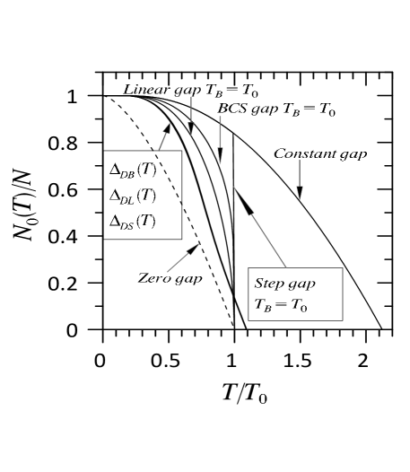
Figure 5: Condensate fractions: the zero gap (IBG) case is in dashed lines; for BCS, step and linear gaps $T_{B}=T_{0}$ was taken; for $\Delta_{DB}(T)$, $\Delta_{DL}(T)$, and $\Delta_{DS}(T)$ gaps the values $T_{B}=10\,T_{0}$, $b=10$, and $T_{D}=0.75\,T_{0}$ were used. For all cases $\Delta_{0}=k_{B}T_{0}$.

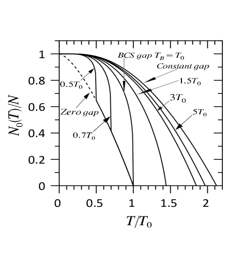
Figure 6: Condensate fraction for BCS gap using $T_{B}=0.5T_{0}$, $T_{B}=0.7T_{0}$, $T_{B}=T_{0}$, $T_{B}=3T_{0}$, and $T_{B}=5T_{0}$ compared to the condensate fraction for zero and constant gap.

In Fig. 5 we show the condensate fractions (CFs) as functions of temperature for the linear, BCS, and step undamped gaps; for all three gaps $\Delta_{0}=k_{B}T_{0}$ and $T_{B}=T_{0}$. We note that from these three gaps, the linear one decreases faster with temperature (see Fig. 1) as well as its CF. These CFs are shown together with that of the zero gap (dashed line)(IBG) and that of the constant gap. Also, in Fig. 5 are shown the CFs for the damped gaps $\Delta_{DB}(T)$, $\Delta_{DL}(T)$, and $\Delta_{DS}(T)$, which merge into one curve from zero to the critical temperature $T_{c}/T_{0}=1.09$, since the three gaps are very similar (see Fig. 2). We note that the CFs do not reach zero with an infinite slope as in the undamped BCS case.

Figure 7: Condensate fraction calculated: with zero gap (dashed line), using $\Delta_{DB}(T)$ gap with $b=10$, $T_{B}=10T_{0}$ and several values of $T_{D}$, from left to right: $T_{D}=0.25T_{0}$, $T_{D}=0.35T_{0}$, $T_{D}=0.50T_{0}$, $T_{D}=0.75T_{0}$, $T_{D}=T_{0}$, $T_{D}=1.50T_{0}$, $T_{D}=2.50T_{0}$. And finally, the condensate fraction calculated with the constant gap $\Delta_{0}=k_{B}T_{0}$.

In Fig. 6 we show the CFs using the BCS undamped gap for several values of $T_{B}$ which we compare with the CFs without gap (IBG) and with a constant gap. For every $T_{B}<T_{0}$, the BEC critical temperature is $T_{0}$, while in the interval of temperatures $T_{B}<T<T_{0}$, the CF curves merge with that of the IBG but for $T\leq T_{B}$ the CF magnitude increases rapidly until it reaches its maximum value $N_{0}/N=1$ at $T=0$, showing a divergent temperature derivative at $T_{B}$ which suggests a second condensation or a two step-condensation Ketterle . Additionally, for $T_{B}>T_{0}$ the BEC critical temperature $T_{c}>T_{0}$, while for $T_{B}>>T_{0}$ the behavior of the CF approaches that of the CF for a constant gap.

In Fig. 7 we plot the CF using the $\Delta_{DB}(T)$ gap for several $T_{D}$ values. For $T_{D}>>T_{0}$ the CF tends to that of a constant gap, while for small values of $T_{D}$ it tends to the case without gap. We note that the discontinuity observed at $T_{B}$ in the derivative for the ungapped BCS case, transforms only into a smooth change of concavity, which avoids touching the CF of the zero gap case. However, for sufficiently small $T_{D}$ the damped-gap curves closely approximate the zero gap curve immediately after the concavity change, as shown by curves $T_{D}=0.25T_{0}$, $0.35T_{0}$ and $0.50T_{0}$. From Fig. 7 we notice that for all the curves the change in concavity shows up at a temperature greater than $T_{D}$ but less than $T_{c}$. Using the damped BCS gap we note that for $T_{D}$ larger than $1.71T_{0}$ we don’t observe a change in concavity as $T_{D}\geq T_{c}$ (see Fig. 4).

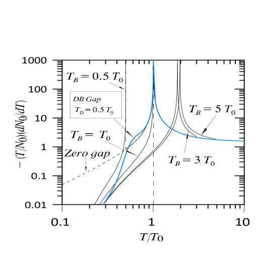
Figure 8: Ratio $-(T/N_{0})dN_{0}(T)/dT$ using the zero gap (short dashed line); the undamped BCS gap for values of $T_{B}/T_{0}=$ 0.5, 1, 3 and 5; and the damped BCS gap for $T_{D}=0.5T_{0}$ (blue line).

Finally, in order to better visualize the divergences in the temperature derivative of the CFs, in Fig. 8 we plot the dimensionless ratio $-(T/N_{0})dN_{0}(T)/dT$ for a Bose gas with zero gap which diverges at the BEC critical temperature $T_{0}$ while for the undamped BCS gaps with $T_{B}\leq T_{0}$ the ratio has two singularities: at $T=T_{B}$ and at $T_{0}$ but, in both cases, for $T>T_{B}$ the ratio returns to the values of the zero gap ones, as is shown for $T_{B}=0.5T_{0}$. When $T_{B}>T_{0}$ the ratio presents only one infinity at its BEC critical temperature $T_{c}>T_{0}$. In the same Fig. 8 we plot a curve for the ratio using a damped BCS gap with $T_{D}=0.5T_{0}$ to show that the infinity observed at $T_{B}$ with the BCS gap, transforms into a simple inflection point at $T_{D}$.

IV.4 Gap effect on the chemical potential

Figure 9: Chemical potential as a function of temperature for BCS, step and linear gaps with different values of $T_{B}$ while for the $\Delta_{DB}(T)$, $\Delta_{DL}(T)$ and $\Delta_{DS}(T)$ gaps, $T_{B}=10T_{0}$.

In Fig. 9 we show the gap effect on the behavior of the chemical potentials as functions of temperature, for all six damped and undamped gaps. For the Bose gas, when $T_{B}=T_{0}$, the chemical potential is the same using any of the undamped BCS, Step, and Linear gaps or using any of the damped $\Delta_{DB}(T)$, $\Delta_{DL}(T)$, and $\Delta_{DS}(T)$ gaps, with $T_{D}=1.5\,T_{0}$. However, using any of the three undamped gaps, when we substitute $T_{B}=3\,T_{0}$ or $5\,T_{0}$ the chemical potential curves merge that of the zero-gap only for temperature $T\geq T_{B}$; at $T_{B}$ the temperture derivative of the chemical potential is infinite.

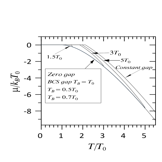
Figure 10: Chemical potential as a function of temperature for BCS gap for several values of $T_{B}$ compared to the zero and constant gap cases.

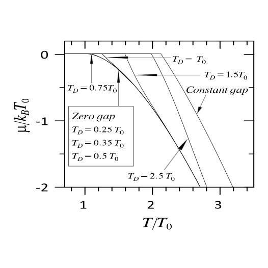
Figure 11: Chemical potential as a function of temperature for $\Delta_{DB}(T)$ gap for several values of $T_{D}$ compared to the zero and constant gap cases.

In Figs. 10 and 11 we show the behavior of the chemical potential as a function of temperature when we use the BCS gap varying the value of $T_{B}$, as well as the $\Delta_{DB}(T)$ gap varying the damping temperature $T_{D}$. For the BCS gap case if $T_{B}\leq T_{0}$ the chemical potential reduces to the gapless case. We do the same for the $\Delta_{DB}(T)$ gap case, but now for $T_{D}$ smaller than $\sim 0.5T_{0}$. If $T_{B}$ or $T_{D}$ take larger values, the chemical potential approaches the constant gap case. Again, the main difference between the BCS and $\Delta_{DB}(T)$ cases is how smoothly their chemical potential curves merge with that for the zero gap.

IV.5 Gap effect on the internal energy

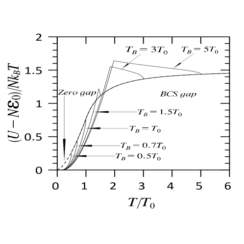
Figure 12: Internal energy divided by $Nk_{B}T$ as a function of temperature for the BCS gap with $T_{B}=0.5\,T_{0},0.7\,T_{0},T_{0},1.5\,T_{0},3\,T_{0}$, and $5\,T_{0}$.

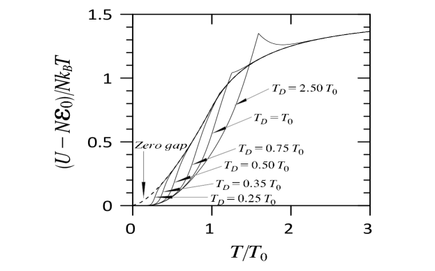
Figure 13: Internal energy divided by $Nk_{B}T$ as a function of temperature using $\Delta_{DB}(T)$ gap with $T_{D}=0.25\,T_{0},0.35\,T_{0},0.50\,T_{0},0.75\,T_{0},T_{0}$, and $2.50\,T_{0}$.

Figure 14: Internal energy using BCS gap with $T_{B}=5T_{0}$. The inset shows a negative infinite slope at $T=T_{B}$.

Figures 12 and 13 show the internal energies divided by $Nk_{B}T$ and referred to the ground state energy $N\varepsilon_{0}$, as functions of temperature for the undamped and damped BCS gaps, respectively. For very large temperatures and every case, the internal energy divided by $k_{B}T$ tends to $3/2$ which is consistent with the energy equipartition principle. In Fig. 12, we show the internal energy divided by $k_{B}T$ using the undamped BCS gap for various values of $T_{B}$ at which there is a discontinuity in its derivative as it merges the zero gap curve, i.e. the derivative is positive infinite for $T_{B}<T_{0}$ and negative infinite for $T_{B}>T_{0}$. In Fig. 14 we plot only the internal energy, i.e. without dividing it by $k_{B}T$, to better visualize its behavior as well as that of its derivative; the inset is a close up of the internal energy curve at $T_{B}$. This strange behavior of the internal energy derivative at $T_{B}$ is not observed using the damped $\Delta_{DB}(T)$ gaps since all curves meet smoothly with the zero gap curve, Fig. 13. We also note that using the undamped gap, for $T_{B}>T_{0}$ the internal energy per particle divided by $k_{B}T$ shows a peak at the corresponding transition temperature from which the internal energy increases more slowly than $k_{B}T$, even though at higher temperatures it grows again. This peak is also observed using the $\Delta_{DB}(T)$ gap, but it gradually disappears as $T_{D}$ decreases.

IV.6 Gap effect on the calculation of the specific heat

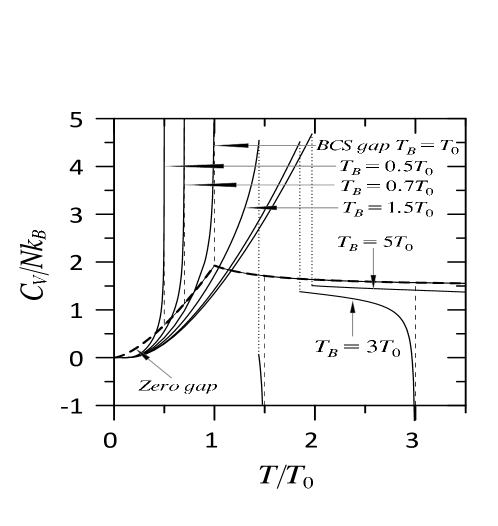
Figure 15: Isochoric specific heat using the BCS gap forh various values of $T_{B}$. As a reference, we also show the specific heat calculated with the zero gap (thick dashed line). Dot lines indicate a jump and thin dashed lines indicate a divergence in the specific heat.

To continue exploring the behavior of thermodynamic properties when the gap has the shape proposed by BCS, we plot the specific heat versus temperature in Fig. 15 for various values of $T_{B}$. For every $T_{B}<T_{0}$, the transition temperature is $T_{0}$ where the specific heat is continuous and shows a peak as well as a positive singularity at $T_{B}$. For $T_{B}>T_{0}$, the specific heat presents a jump at the corresponding transition temperature plus a negative singularity at $T=T_{B}$, which comes from the negative infinite slope of the BCS gap at that temperature.

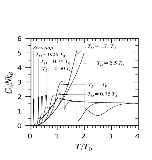
Figure 16: Isochoric specific heat using the $\Delta_{DB}(T)$ gap forh several values of $T_{D}$, besides the gapless case (dashed line). For smaller values of $T_{D}\simeq 0.5T_{0}$ the jump in the specific heat disappears becoming a peak and leaving an additional hump.

To avoid singularities we use the $\Delta_{DB}(T)$ gap instead of the undamped BCS gap, so the infinities observed in Fig. 15 become maximum and minimum values as observed in Fig. 16.

For critical temperature values greater than $T_{0}$ the specific heat has a jump which increases as the critical temperature $T_{c}$ raises until it reaches a maximum at $T_{D}/T_{0}=T_{c}/T_{0}=1.71$. For every $T_{D}\lesssim 0.5T_{0}$, $T_{c}=T_{0}$ and the specific heat has a hump at $T_{D}$ after which it merges the $C_{V}$ curve of the zero gap case.

We note that every $C_{V}$ curve presents an exponential behavior for temperatures near zero, while for much higher temperatures they tend to the 3/2 value.

We observe that although the cases with zero gap and BCS gap with $T_{B}\leq T_{0}$ have the same chemical potential, the behavior of their corresponding $C_{V}$ is very different, i.e., the energy gap has a strong influence on the specific heat behavior, but not on the chemical potential.

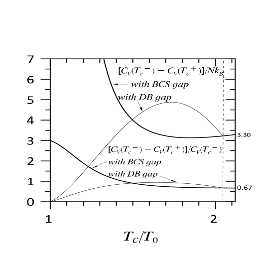
Figure 17: Isochoric heat jump magnitude at the BEC critical temperature $Tc/T_{0}$ as well as its magnitude divided by $C_{V}(T_{c})$, both as functions of $T_{c}/T_{0}$, for the BCS (thick line) and DB gap (thin line) cases.

Finally, Fig. 17 shows the specific heat jump magnitude at the BEC critical temperature $T_{c}/T_{0}$ as well as this magnitude divided by $C_{V}(T^{-}_{c})$, both as functions of $T_{c}/T_{0}$, which were obtained by varying $T_{B}$ for the undamped BCS gap and $T_{D}$ for the DB gap cases. As we increase the values of $T_{B}$ and/or $T_{D}$, the BCS and DB gaps tend to a constant gap $\Delta_{0}$ that corresponds to a BEC critical temperature of 2.12 $T_{0}$ where the values $[C_{V}(T^{-}_{c})-C_{V}(T^{+}_{c})]/Nk_{B}=3.30$ and $[C_{V}(T^{-}_{c})-C_{V}(T^{+}_{c})]/C_{V}(T^{-}_{c})=0.67$. Note that for every $T_{c}\leq T_{0}$, the specific heat shows a zero jump using the damped BCS gap, while using the undamped BCS gap it presents a infinite jump. In adition to this, using the undamped BCS gap the specific heat jump as a function of the BEC critical temperature, decreses untill it arrives to a minimun at $T_{c}/T_{0}=1.85$, for $T_{B}=3\,T_{0}$. While using the damped BCS gap, with $T_{D}=1.75\,T_{0}$ and $T_{B}=10\,T_{0}$, the jump increases from $T_{c}=T_{0}$ till to $T_{c}=1.73\,T_{0}$ where the specific heat jump shows a maximum from where it decreases to reach the value of 3.23 at $T_{c}=2.05\,T_{0}$, which is the maximum critical temperature for $T_{B}=10\,T_{0}$.

V Conclusions

We have given the expressions for the BEC critical temperature, the condensate fraction, the chemical potential, the internal energy and the isochoric specific heat for a 3D Bose gas whose particles have the energy momentum relation $\varepsilon(k)=\varepsilon_{0}+\Delta(T)+\hbar^{2}k^{2}/2m$, i.e., a temperature dependent gap between the ground and the first excited state energies. These expressions are used to calculate the mentioned thermodynamic properties for six gaps: the BCS, Linear and Step gaps, each one in its undamped and damped versions.

To begin with, we confirm that for a temperature independent constant gap: a) All the calculated thermodynamic properties are constant ground state energy $\varepsilon_{0}$ independent, except for the internal energy, which is measured from the reference energy, $N\varepsilon_{0}$, instead of from the zero ground state energy of an IBG, b) A constant gap notoriously increases the magnitude of the BEC critical temperature, where the isochoric specific heat shows a jump, while for $T$ near zero its temperature dependence is exponential rather than proportional to $T^{3/2}$, as for a 3D ideal Bose gas, as already observed in Ref. Martinez-Herrera

The decay of the undamped BCS gap with infinite slope at $T_{B}$ causes abrupt changes in the behavior of the thermodynamic properties of the boson gas as they go through the temperature $T_{B}$. In order to explore the effect of Cooper pairs creation before they reach the BEC critical density we propose a smooth transition from a non-zero gap to an equal to zero one at $T_{B}$, multiplying the undamped BCS gap by an exponential decreasing function of temperature. In this way we prevent the appearence of unwanted infinities in the thermodynamic properties of the Bose gas at $T_{B}$.

For the three types of undamped gaps studied which vanish at $T_{B}\leq T_{0}$, the BEC critical temperature $T_{c}$ is equal to $T_{0}$ and gap shape independent. However, the gap has an important effect on the behavior of the condensate fraction (CF) which, for temperatures $T_{B}<T<T_{0}$, is equal to that of the IBG, while for $0<T<T_{B}<T_{0}$ the rate of accumulation of particles in the ground state shows a sharp increase at $T_{B}$, suggesting a two-step condensation. Also at $T_{B}$ the internal energy shows a peak which turns into a positive infinite divergence in the specific heat. On the other hand, for $T_{D}\lesssim 0.5T_{0}$ the $T_{c}$ equals $T_{0}$ where the CF growths smoothly and remarkably above that of the ideal Bose gas.

The damped gaps become zero at $T_{B}$ which is larger than both $T_{0}$ and $T_{D}$ where the gap magnitude is $\Delta_{0}/2$. For every $T_{D}$ the critical temperature $T_{c}\geq T_{0}$. In addition, the critical temperature as a function of $T_{D}$ is larger than $T_{D}$ untill $T_{D}$ equals $T_{c}$, after which $T_{c}$ becomes smaller than $T_{D}$. The values of $T_{D}$ for which $T_{D}=T_{c}$ depend on the damped gap shape, as shown in the inset of Fig. 4.

Finally, by associating the boson energy gap with a temperature dependence, one can explore how the size of the specific heat discontinuity changes with $T_{c}$.

We thank Dr. P. Salas for her careful reading of the manuscript and her valuable comments. M.A.S. thanks the partial support from grant UNAM-DGAPA-PAPIIT IN114523.

References

- (1) S. Das and S. Sur, Physics of the Dark Universe 42, 101331 (2023); S. Das and R.K. Bhaduri, arXiv:1808.10505v3 [gr-qc] Bose-Einstein condensate in cosmology.
- (2) R. Friedberg and T.D. Lee, Phys. Rev. B 40, 6745 (1989); R. Friedberg, T.D. Lee and H.C. Ren, Phys. Lett. A 152, 417 (1991).
- (3) V.V. Tolmachev, Phys. Lett. A 266, 400 (2000); M. de Llano and V.V. Tolmachev, Physica A 317, 546 (2003).
- (4) F. London, Nature 141, 643 (1938).
- (5) F. London, Superfluids Vol. II (John Wiley & Sons, New York, 1954)p. 53.
- (6) M. Toda, Prog. Theor. Phys. 6, 458 (1951); T. Matsubara, Prog. Theor. Phys. 6, 458 (1951).
- (7) M. Girardeau and R. Arnowitt, Phys. Rev. 113, 755 (1959).
- (8) N. M. Hugenholtz and D. Pines, Phys. Rev. 116, 489 (1959).
- (9) J. García-Nila, M. Sc. (Physics) Thesis, (Universidad Nacional Autónoma de México, Ciudad de México, 2019).
- (10) R. K. Pathria and P. D. Beale, Statistical Mechanics Third Edition (Elsevier, Oxford, 2011), pp. 664-667.
- (11) J.G. Martínez-Herrera, J. García-Nila and M. A. Solís, Phys. Scr. 94, 075002 (2019).
- (12) V. C. Aguilera-Navarro, M. de Llano and M. A. Solís, Eur. J. Phys. 20, 177 (1999).
- (13) N. Doiron-Leyraud, et al., Nature Communications 8, 2044 (2017). DOI: 10.1038/s41467-017-02122-x, www.nature.com/naturecommunications
- (14) R. C. Dougherty, and J. D. Kimel, arXiv-1212.0423-Temperature dependence of the superconductor energy gap.
- (15) W.J. Mullin and A.R. Sakhel, Low Temp. Phys., 166 125 (2012); K. Shiokawa, J. Phys. A: Math. Gen. 33 487 (2000); N.J. van Druten and W. Ketterle, Phys. Rev. Lett. 79, 549 (1997).
- (16) J. S. Kim, B. D. Faeth, and G. R. Stewart, Phys. Rev. B 86, 054509 (2012).
- (17) P. Kapitza, Nature 141, 74 (1938).
- (18) J.F. Allen and A.D. Misener, Nature 141, 75 (1938).
- (19) A. Einstein, Sitzungsberichte der Preussischen Akademie der Wissenschaften 261-267 (1924); A. Einstein, Sitzungsberichte der Preussischen Akademie der Wissenschaften 3-14 (1925).
- (20) W.H. Keesom and H.P. Keesom, Physica 2, 557 (1935).
- (21) R. Kronig and W. G. Penney, Proc. R. Soc. A 130, 499 (1931).
- (22) I. Tamm, Z. Phys. 76, 849 (1932).