Tensor-Aware Energy Accounting

Abstract.

With the rapid growth of Artificial Intelligence (AI) applications supported by deep learning (DL), the energy efficiency of these applications has an increasingly large impact on sustainability. We introduce Smaragdine, a new energy accounting system for tensor-based DL programs implemented with TensorFlow. At the heart of Smaragdine is a novel white-box methodology of energy accounting: Smaragdine is aware of the internal structure of the DL program, which we call tensor-aware energy accounting. With Smaragdine, the energy consumption of a DL program can be broken down into units aligned with its logical hierarchical decomposition structure. We apply Smaragdine for understanding the energy behavior of BERT, one of the most widely used language models. Layer-by-layer and tensor-by-tensor, Smaragdine is capable of identifying the highest energy/power-consuming components of BERT. Furthermore, we conduct two case studies on how Smaragdine supports downstream toolchain building, one on the comparative energy impact of hyperparameter tuning of BERT, the other on the energy behavior evolution when BERT evolves to its next generation, ALBERT.

1. Introduction

Green AI (deep-learning-e-policy, ) is a fundamental challenge with far-reaching implications on the future practice of software engineering, and the sustainability of our society (NSFvmware, ). Deep learning (DL)  (Linnainmaa1976TaylorEO, ; fukushima1980neocognitron, ; bengio2000neural, ; collobert2008unified, ; rumelhart1985learning, ) — the technology that drives the current wave of AI revolution — happens to be excessively energy-hungry. For example, training DL-based large language models is estimated to consume 1,287 megawatt hours of electricity (patterson2021, ). Optimizing the energy consumption of DL systems and applications is a fast-developing direction with intense interest (delight2016, ; neuralpower, ; GARCIAMARTIN201975, ).

The first step toward change is awareness . Underpinning many solutions of energy optimization is the fundamental problem of energy accounting: a deep understanding of energy consumption by breaking it down in (software or hardware) components. This is in contrast with the “monolithic” black-box approach, e.g., measuring the end-to-end energy consumption of a DL training session. Energy accounting is a classic problem, with established solutions (icount, ; currentcy, ; ecosystem, ; chappie, ) focusing on breaking down the energy consumption by hardware components and OS system components. It is not difficult to envision a gray-box approach that retrofits these existing solutions to DL programs, i.e., breaking down the energy consumption of a DL training session by architectural units or OS threads.

Our key insight is that, be it a black-box approach or a gray-box approach, it is a missed opportunity that an energy accounting system ignores the unique abstractions latent in the DL program. After all, a DL program is highly structured, often broken down in modules formed by layers of tensors. Both the black-box approach and the gray-box approach pessimistically treat the DL program just like any other program. How can we leverage the structural information in the DL program for energy accounting? What benefits do we gain with this new flavor of energy accounting?

1.1. Tensor-Aware Energy Accounting

In this paper, we introduce Smaragdine , a novel multi-grained energy accounting system for TensorFlow (tensorflow, )-based DL programs that aligns the decomposition of energy consumption with that of the logical structure of the DL program. At the heart of Smaragdine is a novel white-box methodology of energy accounting: the system is aware of the internal structure of the DL program, and its energy consumption can be broken down following its abstraction boundaries. The output of Smaragdine is a series of nested Energy Distribution Diagrams (EDD) corresponding to the hierarchical decomposition of the DL program. For instance, a top-level EDD shows how the overall energy consumption of a DL program is broken down to modules; the EDDs for sub-modules show how the energy consumption of a particular module is broken down to Deep Neural Network (DNN) layers; and so on. With the hierarchically decomposed EDDs, the atomic unit of energy accounting is a tensor operation in TensorFlow-based implementations.

The white-box approach of Smaragdine has some distinct benefits. First, it complements the active research of explainable AI  (tensorflow, ; sagemaker, ; pace, ) with a perspective on the explainability of non-functional properties such as energy consumption. The hierarchical decomposition structure of EDDs explains how energy consumption is distributed in a layer-by-layer, or even tensor-by-tensor manner. Second, EDDs — with their “logical” nature of energy accounting — may offer insights to downstream designs in energy optimization and energy debugging. With EDDs, it is a trivial task for a downstream designer to zero in on the “energy hotspot” — the highest energy-consuming unit (a module, a layer, or even a tensor) of the DL program. These energy hotspots are likely to be the ideal candidates for optimization or bug fixes due to their proportionally larger impact. Third, the white-box approach of Smaragdine promotes the study of portability in energy accounting. In gray-box approaches, the result of energy consumption is fundamentally platform-specific: the breakdown of energy consumption across hardware components is dependent on what hardware components each platform has. In contrast, Smaragdine breaks down the energy consumption through logical components of a DL program.

The design of Smaragdine must overcome two major challenges. First, there remains a semantic gap between the DL program and the underlying physical system: no ready-made profiler or tool can connect the semantic features of the DL program execution to energy consumption. The solution of Smaragdine is a trace-based alignment algorithm, which conceptually can be viewed as a monitor that simultaneously tracks the DL program runtime events and the energy consumption of the system, and aligns the two to compute the EDD (details in § 3). Second, there are complex interactions at the application-system interface. For example, most TensorFlow applications are multi-threaded running on heterogeneous platforms, i.e. with both CPUs and GPUs. How to account for energy consumption is non-trivial (see § 3 for details).

1.2. Understanding BERT Energy Behavior

To evaluate the effectiveness of tensor-based energy accounting, we apply Smaragdine to BERT (devlin-etal-2019-bert, ), a widely used text analysis model. In the domain of natural language processing (NLP), BERT plays a central role in powering numerous NLP end-user applications. In § 5, we show how the BERT application can be hierarchically decomposed into EDDs. We also show how BERT transformers (transformers, ) — especially its attention modules — dominate the energy consumption in different stages of BERT use, from pre-training to fine-tuning to prediction. Throughout experiments, we find Smaragdine incurs low overhead while retaining high precision and stability.

To further demonstrate the usefulness of Smaragdine in building the downstream toolchain, we use BERT in two case studies. First, we provide a white-box study on the impact of hyperparameter tuning of BERT. We show the energy/power consumption trends with different configurations in the number of layers and the number of hidden embeddings. Second, we conduct an evolutionary study to compare BERT with a newer variant, ALBERT (Lan2020ALBERT:, ). Through Smaragdine, we show how the energy behavior has evolved from BERT to ALBERT.

1.3. Contributions

To the best of our knowledge, Smaragdine is the first white-box energy accounting system for tensor-based DL programs. This paper makes the following contributions:

• the distinct methodology for the energy accounting of DL programs where energy accounting is aware of the internal structure of the DL program, i.e., semantics-aware, illustrated by EDDs (see § 3)

• a trace-based alignment algorithm for bridging the semantic gap of energy accounting while considering complex application-system interactions (see § 3)

• an in-depth evaluation of Smaragdine through BERT, revealing the module-level, layer-level, and tensor-level energy behavior of BERT (see § 5)

• a comparative study on the energy/power impact of hyperparameter tuning in BERT, and the energy/power behavior evolution from BERT to its next generation, ALBERT (see § 6)

Smaragdine is an open-source project. The source code and all raw data of this paper can be found at the anonymous site: https://github.com/project-smaragdine/smaragdine.

2. Background

Deep Learning Programs

A DL program is a dataflow program that composes a number of neural networks (NNs) — and often deep neural networks (DNNs) — together. A neural network (NN) is a collection of neurons wired together, where each neuron serves as a transformation function. Each neuron can be associated with a weight, a potentially adjustable value that indicates the importance of the transformation. DNNs hierarchically organize NNs together, each of which is called a layer. Each DNN layer can be implemented by a tensor (novikov2015tensorizing, ), which generalizes scalar and vector computations over the input/output of the neurons.

Semantically, one may view a DL program as a potentially nested dataflow program. A DL program consists of modules wired together through dataflows, and each module can be implemented either as a tensor, or another (nested) dataflow program. A concretization of this view is to consider a DL program as a “nested DNN,” consisting of layers wired together. Each layer may either be an atomic tensor layer or composite layer, i.e. another DNN. In the rest of the paper, we adopt this view.

DL programs can be trained, i.e., adjusting the neuron weights of its resident NNs to fit a data set. Once trained, a DL program can be used for prediction, i.e., estimating an output from an input. DNNs are trained through backpropagation (Linnainmaa1976TaylorEO, ; rumelhart1985learning, ), where the error of the model’s prediction is used to adjust weights. This requires computation of the network’s gradient – the differential impact of neuron connections – to correctly adjust the weights.

BERT

BERT (devlin-etal-2019-bert, ) is a tunable NLP model relying on DNNs. BERT popularized the idea of splitting training into two stages: pre-training and fine-tuning. BERT is initially pre-trained on a general data set – where all model weights are trained for a long time. BERT can then be fine-tuned on a curated data set – where only a subset of model weights are trained for a shorter time. As a result, BERT can be quickly configured to solve specific kinds of text problems without retraining from scratch (devlin-etal-2019-bert, ; patent-bert, ; bio-bert, ), leading to a break-through in NLP.

For NLP models, two important tasks are embedding and encoding. Embedding represents the input (such as a text) for processing, and encoding addresses the transformation between the input and the output. In design, BERT’s encoding module, called an encoder, is a nested DNN: it stacks together a number of modules (i.e., composite layers) each of which is called a transformer (transformers, ). For our purpose, note that a transformer is a nested dataflow program with NNs inside. A key BERT innovation is one of the NNs nested inside a transformer, called self-attention. This unit enables a (now widely used) form of encoding known as bidirectional representation.

TensorFlow

TensorFlow (tensorflow, ) is a machine learning library that supports complex tensor calculus. TensorFlow programs can be designed using the Keras API, a framework for constructing DL programs. For DL training, computing the gradient by hand is non-trivial. To overcome this, TensorFlow automates this process by using automatic differentiation (Linnainmaa1976TaylorEO, ).

3. Smaragdine Design

3.1. Problem Statement

We use $l\in\mathbb{LN}$ represent layer names, $t\in\mathbb{TN}$ tensor (layer) names, and $c\in\mathbb{CN}$ composite layer names. $\mathbb{LN}=\mathbb{TN}\cup\mathbb{CN}$. We further use $\mathbb{TO}$ to represent the set of tensor operations.

Definition 3.1 (DL Program).

We define a program $P\in\mathbb{P}$ as a directed graph $\langle N;E\rangle$ where $\emph{N}=\emph{C}\cup\emph{T}$, and $\emph{C}:\mathbb{CN}\rightharpoonup\mathbb{P}$ is a bijective partial function for the set of composite layers, $\emph{T}:\mathbb{TN}\rightharpoonup\mathbb{TO}$ is a bijective partial function for the set of tensor layers, and $E:\mathbb{LN}\rightharpoonup\mathbb{LN}$ is a partial mapping denoting the dataflow among layers.

The primary goal of Smaragdine — i.e., tensor-level energy accounting — is to produce an EDD:

Definition 3.2 (Energy Distribution Diagram).

We define an $\emph{EDD}\in\mathbb{EDD}$ as a directed graph $\langle\mathcal{N};E\rangle$ where $\mathcal{N}=\mathcal{C}\cup\mathcal{T}$, and $\mathcal{C}:\mathbb{CN}\rightharpoonup\mathbb{EDD}$ is a partial function for the set of EDDs (indexed by composite layer names), $\mathcal{T}:\mathbb{TN}\rightharpoonup\mathbb{ENERGY}$ is a partial function for the set of energy consumption values (indexed by tensor names).

It is important to observe that the structure of an EDD in Def. 3.2 mirrors that of the DNN program in Def. 3.1. This is intentional: it is the goal of Smaragdine that the output of energy accounting reflects the logical structure of the DNN program.

Most DL programs rely on a very limited set of tensor operations, i.e., the sizes of $\mathbb{TN}$ and $\mathbb{TO}$ are small. For example, BERT is built on top of a limited number of tensor operations, such as vector multiplication (MATMUL) and tangent gradient (TANHGRAD). However, it is important to note that where tensors appear in the DL program makes them semantically different: a vector multiplication used for computing self-attention is different from one using Einstein summation. To effectively support this difference, we introduce qualified tensor name $(q\in\mathbb{QN})$, in the form of $\langle[c_{1},\dots,c_{n}];t\rangle$ for some $n\geq 0$. Intuitively, this refers to a tensor named $t$ that immediately resides in layer $c_{n}$, which is in turn nested in $c_{n-1}$ and so on.

Example 3.3 (Qualified Tensor Name and its ShortHand).

The QTN $\langle\texttt{[bert, encoder, layer\_0, output, dense]};\texttt{ MatMul}\rangle$ refers to tensor MatMul defined in the dense layer, which in turn is nested in the output layer, which is nested in layer_0, and so on. From now on, we use its more mnemonic shorthand form  bert/encoder/layer_0/output/dense/MatMul.

With the QTN, we can now “flatten” the EDD to produce a representation more friendly for tensor-level comparison of energy consumption:

Definition 3.4 (Tensor Energy Footprint).

We define a tensor energy footprint (TEF) $F$ as a function $TEF:\mathbb{QN}\rightharpoonup\mathbb{ENERGY}$.

Given a program $P$, the transformation between EDD and TEF is simple, to be defined in § 3.3.

3.2. Algorithm Overview

Design Challenges

As we discussed in § 1, Smaragdine first must overcome a Semantic Gap challenge: while it is generally known how to perform (gray-box) energy accounting in a per hardware component or per thread manner, how such systems-level energy consumption can be mapped to the structure of the DL program is an open question. Secondly, there is an Application-Systems Interface challenge. A typical DL program is multi-threaded, so addressing concurrency is the rule not the exception; DL programs routinely run in a heterogeneous environment – where there may be multiple devices, such CPUs and GPUs. This complicates accounting further as device reports their consumption separately.

A Solution Overview

To address the Semantic Gap challenge, Smaragdine is designed as a runtime monitor to perform trace-based alignment: it collects two traces of information at time intervals, and align them based on timestamps. The two conceptual traces are (1) a tensor event trace $\tau:\mathbb{TIMESTAMP}\rightharpoonup\mathbb{QTN}$, which temporarily records the tensor activities, where each tensor is identified by its QTN; (2) a power trace: $\pi:\mathbb{TIMESTAMP}\rightharpoonup\mathbb{POWER}$. The core algorithm is conceptually simple: Smaragdine continuously tracks what tensor events have happened, where each event has happened, and how much power the device has when it happens. Now that $\tau$ contains the semantic information, its alignment with $\pi$ bridges the semantic gap between the program runtime and the system runtime. Let us now overview several technical challenges:

• Imperfect Alignment: It should be known that neither $\tau$ nor $\pi$ is surjective; in other words, some timestamps may not have a tensor event or any power reading. In a nutshell, Smaragdine is a recency-based alignment algorithm: we align a tensor event with the most recent power reading in the time line.

• Multiplicity: $\pi$ is not injective; in other words, there might be multiple tensor events that occur at the same timestamp. In Smaragdine, all tensor events that happen at the same time are attributed with an equal share of the energy consumption.

• Durable Events: tensor events happen for a duration. This realistic view is in contrast with our conceptual formulation above, where the $\tau$ mapping appears to indicate that the occurrence of a tensor event happens at an instantaneous timestamp. We resolve this with a conceptual algorithm (in Algorithm 2) and an optimized algorithm (see discussion in § 3.3).

To address the Application-System Interface challenge, Smaragdine behaves as a universal accountant, abstracting the system’s consumption as energy traces. First, Smaragdine is aware of the heterogeneity of the system, where trace alignment is performed in a per device manner. In other words, Smaragdine operate on the device tensor event trace $\theta:\mathbb{DEVICE}\rightharpoonup\tau$, and the device power trace: $\epsilon:\mathbb{DEVICE}\rightharpoonup\pi$. Second, Smaragdine is aware of the concurrency of the system. With Multiplicity, the tensor events that are concurrently executed on different threads residing on one device each will receive an equal share of the energy consumption of that device. Smaragdine also addresses complex systems behavior such as thread migration, where the mapping between threads and devices is updated.

3.3. Algorithm Specification

Key Data Structures

Algorithm 1 Smaragdine Data Types

1typedef  Ts  Int // time stamp

2typedef  Dur  Int // time duration

3$\textbf{typedef}\ \textsc{Device}\ \textbf{enum}\ \{$

4    $\textsc{CPU\_0},\textsc{CPU\_1},...$

5   $\textsc{GPU\_0},\textsc{GPU\_1},...$

6$\}$

7typedef  Op  Int // ID of a tensor operation

8$\textbf{typedef}\ \textsc{Event}\ \textbf{struct}\ \{$

9    $\texttt{ts}:\textsc{Ts}$ // event start time

10   $\texttt{dur}:\textsc{Dur}$ // elapsed time for event

11   $\texttt{device}:\textsc{Device}$ // executing device

12   $\texttt{op}:\textsc{Op}$ // event operation

13$\}$

14$\textbf{typedef}\ \textsc{EventTrace}\ \textsc{List}\langle\textsc{Event}\rangle$

15typedef  Energy  Float // energy in joules

16typedef  Power  Float // power in watts

17$\textbf{typedef}\ \textsc{PowerTrace}\ \textsc{Map}\langle\textsc{Ts},\textsc{Power}\rangle$

18$\textbf{typedef}\ \textsc{DevicePowerTrace}\ \textsc{Map}\langle\textsc{Device},\textsc{PowerTrace}\rangle$

19function Start() // begin accounting

20function Stop() : DevicePowerTrace // stop accounting and obtain traces since start

21function Now(T: Ts, TL : $\textsc{Set}\langle\textsc{Ts}\rangle$) : Ts // retrieves the largest time stamp from a set which is smaller than a given time stamp

22  $\textbf{return}\ \textsc{Max}(\texttt{ts}\in\texttt{TL}\ \textbf{where}\ \texttt{ts}<=T)$

Algorithm 1 presents the key data structures Smaragdine works with at run time. The $\tau$ and $\pi$ traces we discussed in the previous section are represented by EventTrace and PowerTrace respectively. Due to Multiplicity, the EventTrace also records the duration of the tensor event (dur), together with its starting time (dur), as shown in Lines 9-13. The QTN of the tensor operation is kept in the op field. To address the Application-Systems Interface challenge, we also record where in the underlying systems such event is happening, in the device field. Possible values are the CPU/GPU units, as shown in the enum definition for Device. Smaragdine provides Start and Stop methods (Lines 19- 20) to enable an accounting session. Due to the need for Imperfect Alignment, utility function Now returns the last interval timestamp that is still smaller than the given timestamp.

TEF Computation

Algorithm 2 Smaragdine Accounting

1$\textbf{typedef}\ \textsc{DeviceFlatTrace}\ \textsc{Map}\langle\textsc{Device},\textsc{Map}\langle\textsc{Ts},\textsc{Set}\langle\textsc{Op}\rangle\rangle$

2function Flatten(T : EventTrace) : DeviceFlatTrace

3  $\texttt{ft}\leftarrow\textbf{new}\ \textsc{DeviceFlatTrace}$

4  for e  in  T do

5   for $\texttt{t}\ \textbf{in}\ \textsc{Range}(\texttt{e.ts},\texttt{e.ts + e.dur + 1})$ do

6    $\texttt{ft}[\texttt{e.device}][\texttt{t}]\stackrel{{\scriptstyle+}}{{\leftarrow}}\texttt{e.op}$      

7  return  ft

8

9$\textbf{typedef}\ \textsc{TEFootprint}\ \textsc{Map}\langle\textsc{Op},\textsc{Energy}\rangle$

10$\textbf{typedef}\ \textsc{TsFootprint}\ \textsc{Map}\langle\textsc{Ts},\textsc{TEFootprint}\rangle$

11function BuildTEFootprint(OP : $\textsc{Set}\langle\textsc{Op}\rangle$, P : Power) : TEFootprint

12  $\texttt{of}\leftarrow\textbf{new}\ \textsc{OpFootprint}$

13  for op  in  OP do

14   $\texttt{of}[\texttt{op}]\leftarrow\texttt{P}\ /\ \texttt{|ops|}$   

15  return  of

16

17function GenFootprint(T : EventTrace, DPT : DevicePowerTrace) : TsFootprint

18  $\texttt{tf}\leftarrow\textbf{new}\ \textsc{TsFootprint}$

19  $\texttt{ft}\leftarrow\textsc{Flatten}(\texttt{T})$

20  for $\texttt{d}\in\textsc{Dom}(\texttt{t})$ do

21   for $\texttt{ts}\in\textsc{Dom}(\texttt{ft}[\texttt{d}])$ do

22    $\texttt{ops}\leftarrow\texttt{ft}[\texttt{d}][\texttt{ts}]$

23    $\texttt{p}\leftarrow\texttt{DET}[\texttt{d}][\textsc{Now}(\texttt{ts},\textsc{Dom}(\texttt{DPT}[\texttt{d}]))]$

24    $\texttt{tf}[\texttt{ts}]\leftarrow\textsc{BuildTEFootprint}(\texttt{ops},\ \texttt{p})$      

25  return  f

26

27function Aggregate(TF : TsFootprint) : TEFootprint

28  $\texttt{of}\leftarrow\textbf{new}\ \textsc{TEFootprint}$

29  for $\texttt{ts}\ \textbf{in}\ \texttt{x}\in\textsc{Dom}(\texttt{TF})$ do

30   for $\texttt{op}\in\textsc{Dom}(\texttt{TF}[\texttt{ts}])$ do

31    $\texttt{of}[\texttt{op}]\stackrel{{\scriptstyle+}}{{\leftarrow}}\texttt{TF}[\texttt{ts}][\texttt{op}]$      

32  return  f

33

Algorithm 2 specifies the core monitoring algorithm which ultimately produces the TEF. Due to the technical challenge of Durable Events, we flatten the EventTrace, i.e., turning it into a DeviceFlatTrace where the event is repeated for every interval covered by the duration The flatten function iterates through EvenTrace events and add them to a DeviceFlatTrace from the start to the end of the event (Lines 2 - 8). Finally, we account operations by iterating over each device’s DeviceFlatTrace. The tensor operations for each time interval is assigned an equal fraction of the total energy. The TEF, represented in the algorithm as TEFootprint, is Aggregated together by combining all TSFootprint’s.

The algorithm implemented by Smaragdine is an optimized version of Algorithm 2. In practice, if a tensor operation has a long duration, the Flatten process in Algorithm 2 would require insert many entries in DeviceFlattenTrace. Our optimized algorithm keep track of the start/end timestamps of a tensor operation internally without an explicit flattening process. The specification of this optimized algorithm can be found in the repository.

EDD Reconstruction

Given a TEF, it is simple to compute a corresponding EDD. Function $\emph{T2E}(F,P)$ computes the EDD for program $P$, defined as $\langle\mathcal{N};E\rangle$, where $\mathcal{N}$ is the smallest set such that $\mathcal{N}(c_{1})(c_{2})\dots(c_{n})(t)=F(q)$ for any $q\in\emph{domain}(F)$, $q=\langle[c_{1},\dots,c_{n}],t\rangle$, where $P=\langle\emph{N};E\rangle$.

Summarized TEF

Realistic DNN programs have a complex topology. This implies that a typical TEF in the real world contains numerous entries. From the standpoint of program understanding, it would be desirable if we could combine the energy consumption of “similar” tensors together.

For transformer-based DNN programs such as BERT, an opportunity exists: while such programs consist of a large number of transformers, the internals of all transformers are self-similar, i.e., they have indistinguishable topology (HOFMANN2003155, ). This provides us an opportunity to sum up the energy consumption of all tensors that reside in self-similar transformers. In BERT, the boundary of a transformer is identified by module name $\texttt{layer}\_i$, where $i$ is a number that ranges the number of transformers. In other words, we can potentially sum up the following entries in a TEF:

bert/encoder/layer_0/output/dense/MatMul $\mapsto$ 5

bert/encoder/layer_1/output/dense/MatMul $\mapsto$ 3

…

into one entry:

bert/encoder/transformer/output/dense/MatMul $\mapsto$ 8

Definition 3.5 (Summarized Tensor Energy Footprint).

A summarized tensor energy footprint (STEF), represented as $S:\mathbb{SQ}\rightharpoonup\mathbb{ENERGY}$, maps summarized qualified tensor name (SQTN) to energy consumption values. An SQTN $\emph{sq}\in\mathbb{SQ}$ has the structure of $\langle[s_{1},\dots,s_{n}];t\rangle$ where $\{s_{1},\dots,s_{n}\}\subseteq\mathbb{CN}\cup\{\texttt{transformer}\}$.

Computing an STEF from a TEF is simple. Given a TEF $F$, function $\emph{T2A}(F)$ compute $S$ as the smallest set s.t. $S(\emph{sq})={\displaystyle\sum_{\emph{sq}=\diamond(q)}F(q)}$ where $\diamond(q)=q[\texttt{layer}\_1\mapsto\texttt{transformer},\dots,\texttt{layer}\_n\mapsto\texttt{transformer}]$.

In addition, Smaragdine can also produce the power counterpart of STEF, which we call Summarized Tensor Power Footprint (STPF). We elide their verbose definitions in this presentation.

4. Smaragdine Implementation

Decoupled Monitoring

We choose to implement Smaragdine as a separate process co-running with the monitored application. In our implementation, Smaragdine is written in Rust. The monitored TensorFlow applications we evaluate Smaragdine over are Python runtimes. The inter-runtime communication is implemented through grpc , a widely used language-agnostic remote procedure call framework. At the begin and end of the training epochs in TensorFlow, we use SessionRunHook to attach callbacks to asynchronously communicate with Smaragdine. The Start and Stop methods of Smaragdine are called upon receiving the grpc messages. Decoupled monitoring enables a more language-neutral approach toward the monitored application, anticipating the diversity of future ML applications, which may be written in other languages.

Power Sampling

Smaragdine samples the power consumption of all CPU/DRAM/GPU components of the underlying system. The power trace is broken down by device, as described at line 4 Algorithm 2.

Specifically, the CPU and DRAM energy consumption is obtained through Intel’s RAPL interface. RAPL provides Machine-Specific Registers (MSR) to report the accumulative energy consumption of Intel processors, reporting for each domain (i.e., motherboard socket) separately. Within each domain, it further breaks down the report by components, i.e., the CPU cores, the uncore (cache, TLB, etc), and the DRAM regulator. The MSR is read through powercap, a Linux power management module where MSR values are exposed as a psuedo-filesystem.

GPUs energy consumption is obtained through the NVIDIA Management Library (NVML) , an interface for both monitoring and managing NVIDIA devices. The NVML provides high-level querying of GPU devices, including the instantaneous power. Smaragdine samples from the NVML using the nvml-wrapper package , which provides a thin Rust wrapper around the library.

Our power sampling period is set at 4 milliseconds, which is the smallest period that we observe where power data are updated in hardware.

Excluding Energy Consumption by OS and Smaragdine

One practical concern is that the OS maintains a basic level of energy consumption, such as through daemons. In a similar vein, Smaragdine as a co-running process also incurs a small share of energy consumption itself. We need to exclude the energy consumption resulting from the processes outside of our application, including the co-running Smaragdine process. We resort to a prior tool Eflect to accomplish this goal. Eflect was able to virtualize the energy consumption, i.e., separating the fraction of energy consumption due to a specific application from the rest of the system. In other words, for each power sample obtained by Smaragdine at line 19 in Algorithm 1, the sample only consists of the fraction of energy consumption due to the monitored application itself. We do not virtualize the energy consumption of the GPUs. Unlike the CPUs, GPUs only execute the kernel required by our monitored application, without the background OS daemon processes. The Smaragdine process itself does not execute on the GPU.

Event Trace Collection

We obtain the TensorFlow event trace through TensorFlow’s built-in profiler. The profiler monitors the application with callbacks to the start and end of all operations executed. We start the profiler through the ProfilerHook class, an extension of the SessionRunHook. At the end of execution, the profiler produces an event trace using TensorFlow’s timeline API, where events are identified by the tensor’s QTN. Combined with traces from the Smaragdine hook described above, we account the epoch with Algorithm 2.

5. Evaluation

We present an experimental evaluation of Smaragdine with the aim to answer the following questions:

• RQ1: what insights can Smaragdine provide to the designers of DL applications on their energy consumption?

• RQ2: what are the precision, overhead, and scalability characteristics of Smaragdine-based energy accounting?

• RQ3: can Smaragdine help build the downstream toolchain for understanding DL applications?

We answer RQ1 and RQ2 in this section, and RQ3 in § 6.

5.1. Experimental Setup

All experiments are conducted on a server consisting of an Intel Xeon Silver 4300 v3 2.30 GHz CPU with 20 cores, a PNY NVIDIA Quadro P5000 GPU with 2560 CUDA cores, and 64GB DDR4 of RAM. The CPU is configured with hyperthreading enabled. The machine runs with a Debian 11 OS with the default ondemand governor where the P-state is on. All experiments were run with TensorFlow 2.8 on Python 3.8. We use BERT through its experiment repository . Both pre-training and fine-tuning were performed for 500 epochs with the BERT repository’s recommended parameters:

• A max sequence length of 128 words

• A training batch size of 32 records

• A learning rate of $2\times e^{-5}$

BERT is pre-trained with BookCorpus, a collection of free, unpublished novels, and English Wikipedia, which contains annotated entries from a variety of domains. BERT is fine-tuned with the Corpus of Linguistic Acceptability (CoLA) (warstadt2018neural, ) data set. Each experiment described in this paper is repeated 5 times.

5.2. A Bird’s Eye View of BERT’s Energy Consumption

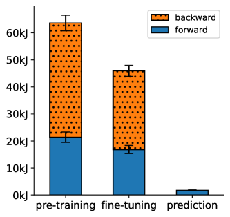
Figure 1. BERT Total Energy Consumption (The forward and backward passes are shown as stacked bars. Throughout the paper, the whiskers show the standard deviation.)

Recall from § 2 that BERT operates in three stages — pre-training, fine-tuning, and prediction. Smaragdine is capable of performing energy accounting for all 3 stages. For pre-training and fine-tuning, we further separate each into the forward and backward passes of the execution, following our discussion in § 2.

Fig. 1 provides a high-level comparison on the energy consumption of the 3 stages. Here, pre-training is shown as the most expensive, consuming over 60 KJs, vs. fine-tuning’s 45KJ consumption. This observation is aligned with our understanding of BERT: pre-training updates more neurons than fine-tuning. Prediction consumes very little energy, around 2KJs. Prediction does not require the machinery of training, such as batching and iterative execution. As a result, we expect prediction to be the cheapest task.

Since pre-training is the largest consumer, as well as the first step in building a model, we will present our results of energy accounting of this stage for the rest of this section. The results for other stages are provided in the public repository (https://github.com/project-smaragdine/smaragdine).

5.3. Multi-Grained Energy Accounting

Smaragdine is able to report energy consumption of a DL program following the logical structure of its hierarchical decomposition:

• (whole) program-level accounting. At the top level, Smaragdine can provide an overview of how the energy consumption of the program is distributed among its top-level layers. For example, Fig. 2 is an EDD that shows the top-level view of BERT energy consumption.

• (composite) layer-level accounting. Smaragdine can show the energy consumption of a composite layer through nested EDDs. For example, Fig. 2 shows the EDD of BERT’s encoder layer. Fig. 4 shows a set of hierarchical views of the first transformer — a composite layer in the encoder — and its components.

• tensor-level accounting. At this fine-grained level, Smaragdine reports the energy consumption of tensors, i.e., the “leaves” in the hierarchical decomposition structure. Fig. 5 shows an STEF that provides a summarized view where the energy consumption of tensors is ranked.

5.3.1. Program-Level and Top-Layer-Level Accounting

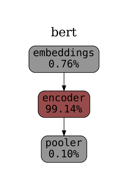
(a) EDD for bert

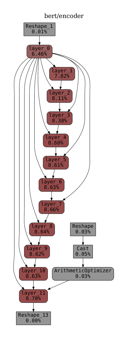
(b) EDD for bert/encoder

Figure 2. Program-Level and Encoder-Level EDDs for BERT’s Forward Pass during Pre-Training (The left figure shows the top-level view, and the right figure shows the encoder layer view. The number in each box is the normalized energy consumption of the boxed unit relative to that of all boxes in the same figure. The relative values of these numbers are also represented by color intensity: a box in a more vibrant color indicates higher energy consumption. A round-edged box represents a composite layer, while a sharp-edged one represents a tensor (layer). Arrows indicate the dataflow.)

In Fig. 2, we first present program-level accounting for BERT, and the accounting for its most energy-consuming top-layer, encoder. Smaragdine is capable of performing accounting separately for its forward pass and its backward pass. The shown EDDs show the forward pass. The results for the backward pass are deferred to our repository, with similar trends as discussed below.

There are two key observations. First, the encoder and its enclosing transformers dominate the energy consumption of BERT. BERT has two main tasks: embedding and encoding. As it turns out, the latter consumes more than 99% of BERT energy consumption. With the encoder, the stacked transformers again dominate the energy consumption. Given the central role that transformers play in language models like BERT, this comes with no surprise. Second, the transformers do not consume energy uniformly. The transformers closer to the input are lower consumers, up to 2% less than the average consumption of 8.25$\pm$0.61%. The consumption rises until plateauing around 8.55% at the fifth transformer. We speculate that this is due to the power state of the executing devices. To confirm this, we investigated the power trace of the underlying system, with results shown in Fig. 3. The TensorFlow runtime appears to schedule the transformer execution in phases, where the first transformer is executed in the earlier timestamps in each training epoch. Interestingly, the CPU/GPU system starts at a lower-power state, and only ramps up when the workload increases. As a result, operations executed in the early phases (such as the first transformer) consumes less energy overall.

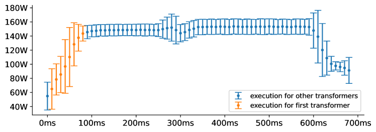
Figure 3. BERT Single-Epoch Power Trace (The X-axis is elapsed time and the Y-axis is the power consumption. Each point in the figure is the average of power consumption of all training epochs at the same elapsed time. The orange data points show the time stamps when the first transformer is executed, while those in blue show the time stamps when other transformers are in execution.)

(a)

(b)

(c)

(d)

Figure 4. Transformer-Level EDDs for the Forward Pass of BERT’s First Transformer (bert/encoder/layer_0) and its Nested Layers.

5.3.2. Energy Accounting for Nested Layers

Based on our earlier discussion, transformers are the largest consumers in BERT. We use Smaragdine to “zoom in” deeper in the hierarchy, to the first transformer (bert/encoder/layer_0). Fig. 4a shows its EDD.

Two observations are noteworthy. First, the attention layer consumes a significant amount of energy; in addition, the attention layer’s energy is primarily consumed in computing self-attention (self). This confirms the important role that the attention mechanism plays in BERT. Second, dense computation dominates the energy consumption. Through the EDDs of the sub-layers in Fig. 4b,  4c, and  4d, we can observe that the dense layers inside intermediate and output dominate the energy consumption. The dense layers are implemented as matrix multiplication, one of the most computationally intensive operations.

The forward pass and the backward pass exhibit similar energy behavior (EDDs in the repository), with one notable exception: the attention layer consumes a noticeably larger share in the backward pass, 48.19%, than the forward pass of 40.68%. This share difference also persists in the self-attention layer: the shares for the backward pass vs. the forward pass are 79.52% vs. 72.51%. In the backward pass, gradient calculation is relatively expensive for attention layers.

5.3.3. Tensor-Level Accounting

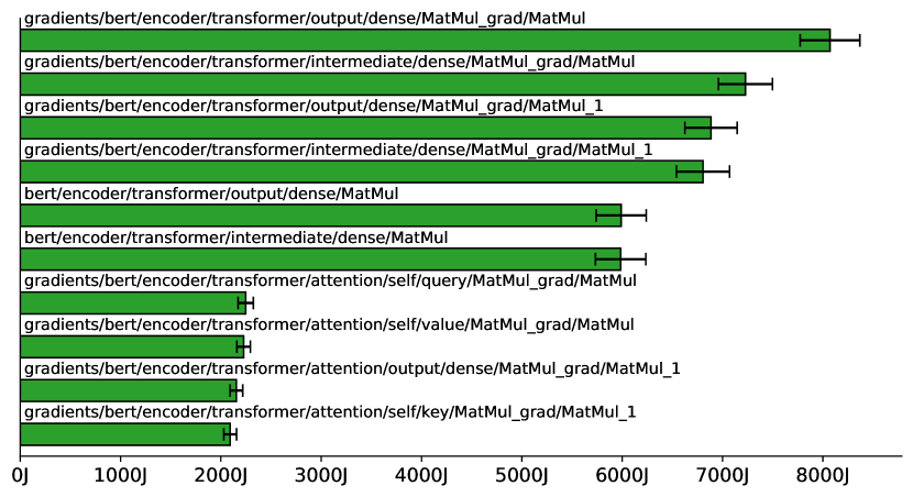
(a) STEF

(b) STPF

Figure 5. Top Energy/Power-Consuming Tensors through STEF and STPF (The QTN is above each bar.)

Fig. 5 presents the top-10 tensors in the form of STEF and STPF. Here, we highlight 2 observations. First, matrix multiplication dominates the energy consumption. All top-10 energy-consuming tensors are vector multiplication across different BERT layers. Second, the backward pass is a much larger consumer than the forward pass. In BERT, all backward passes are included in the top composite layer of gradient. Here, 8 of 10 of the top energy-consuming tensors come from the backward pass. This is consistent with the top-level view we showed in Fig. 1, but the STEF here provides a significantly finer-grained view on which tensors that contribute to the larger energy consumption. Third, the power consumption of different tensors remains stable. Indeed, regardless of the different semantic purposes that different tensor computations serve, all share the nature of matrix multiplication (MatMul). As power consumption is strongly correlated with the nature of the computation itself, the power remains similar for all MatMul tensors.

5.4. Intrinsic Characteristics

5.4.1. Precision

For all sampling-based systems, the precision of the results may be impacted by the sampling design itself, such as how many and how often samples are taken. We evaluate the precision of Smaragdine in two metrics: accounting similarity with sample sparsing (ASSS) and accounting similarity with sample widening (ASSW). Common to the two metrics is the notion of accounting similarity, defined as the Pearson Correlation Coefficient (PCC) of two STEFs resulted from two instances of Smaragdine, indexed by the tensor IDs. We show an example in Fig. 6. Intuitively, a higher value of accounting similarity implies two accounting results demonstrate more similar trends.

	STEF1	STEF2
Input Embedding	21J	15J
Output Embedding	21J	15J
Input Attention	54J	23J
Output Attention	54J	23J
Input Add & Norm 1	118J	59J
Output Add & Norm	118J	59J
Input Feed Forward	184J	92J
Input Add & Norm 2	100J	50J
Output Feed Forward	200J	100J

$\rightarrow$ 0.9958

Figure 6. Accounting Similarity (STEF₂ has half the sampling rate of STEF₁. The PCC of the two STEFs is shown to the right.)

ASSS is built upon the intuition that the ground truth is approached when the sampling rate reaches infinity. Recall in § 4, power consumption is sampled at four milliseconds, and cannot be sampled at a higher rate due to hardware constraints. We circumvent this challenge by computing the accounting similarity when the sampling interval is further lengthened. This counter-intuitive idea is rooted on how discrete systems approximate continuous values: if we view the result when the sampling rate is infinity as the limit, the shape of the trajectory where the limit is approached offers clues on the error of the approximation. The results are shown in Fig. 7a. The similarity oscillates between 0.90 and 0.94. Overall, the curve forms a “plateau”: further increasing the sampling rate would likely offer little benefit in changing the trend exhibited in the STEFs.

(a) ASSS

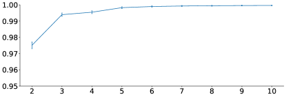
(b) ASSW

Figure 7. ASSS and ASSW (In the left figure, the X-axis is the sampling period and the Y-axis is the ASSS value. In the right subfigure, the X-axis is the number of experiments, and and the Y-axis is ASSW value. The PCC is computed between the STEF of Smaragdine’s default setting, and that of the setting in the X-axis.)

The intuition behind ASSW is that the ground truth of a sampling-based algorithm can be approached when the number of samples reach infinity. Recall that each Smaragdine experiment is repeated in 5 runs (see § 5.1). We now compute ASSW by relating the STEF generated when 2, 3, 4, 5, etc, experiments are conducted, i.e., in 10, 15, 20, 25 runs. The results are shown in Fig. 7b. The similarity is high, between 0.97 and 0.99.

5.4.2. Stability

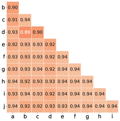
Figure 8. Accounting similarity across Experiments (Each box is the PCC between two experiments indexed by a-i. Each experiment is the default 5-run by Smaragdine. )

In addition to precision, a sampling system must preserve stability: when the same experiment is repeated, a stable sampling system should produce consistent results.

To evaluate this, we can compute the accounting similarity between different experiments, shown in Fig. 8. All pairs of experiments have a high accounting similarity. Generally, a PCC greater than 0.7 is considered to be strong correlation.

5.4.3. Overhead

Finally, we quantify the overhead Smaragdine introduces to the application under energy accounting. We compare the application under Smaragdine’s accounting with the same application without accounting. We report a runtime overhead of $-0.052\pm 0.12\%$ and an energy overhead of $0.47\pm 1.10\%$. The overhead is well within the margin of errors. Smaragdine is a low overhead energy accounting system.

6. Case Studies

In this section, we describe two cases studies that demonstrate the usefulness of Smaragdine for supporting client studies of DL energy consumption. This section is aimed at addressing RQ3.

6.1. A Comparative Study on BERT Variants

As shown by the original developers of BERT (devlin-etal-2019-bert, ), BERT can be configured with different hyperparameter settings. In particular, there are two important ones that impact the model topology: the number of stacked transformer layers (L), and the number of hidden embeddings (H). Our analysis in §. 5 was applied to the largest model described in the original paper, i.e. $\textsc{BERT}{}_{\textsc{BASE}}:$ L=12, H=768.

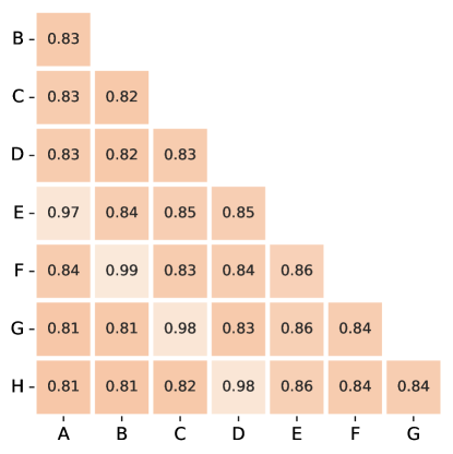
(a) Power PCC

(b) Energy PCC

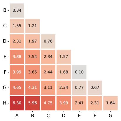
(c) Power MED

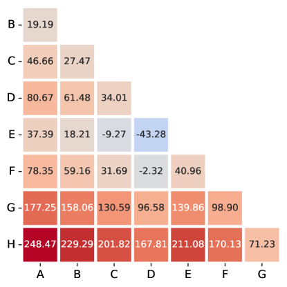
(d) Energy MED

Figure 9. A Comparative Study on BERT Hyperparamter Tuning (In the first/second sub-figures, each box shows the PCC between two STPFs/STEFs produced for two BERT variants by Smaragdine. In the third/fourth sub-figures, each box shows the mean error difference (MED) between two STPFs/STEFs produced for two BERT variants by Smaragdine. For MED, the variant on the Y-axis subtracts the one on the X-axis. For readability, red/blue colors indicate positive/negative numbers, and color intensity indicates the absolute values of the numbers. Each letter corresponds to a specific hyperparameter setting (A: [L=6, H=512], B: [L=8, H=512], C: [L=10, H=512], D: [L=12, H=512], E: [L=6, H=768], F: [L=8, H=768], G: [L=10, H=768], H: [L=12, H=768]).

We use Smaragdine to generate the STEFs and STPFs for BERT under alternative hyperparameter settings, with the comparative results shown in Fig. 9. Specifically, Fig. 9a and  9b show high PCC correlation across all variants in terms of both power and energy. This means that the relative standing of power/energy consumption of different tensors remains stable across different BERT variants. In other words, the top-consuming tensors in one BERT variant are likely the top-consuming tensors in the others too.

Fig. 9c and  9d show the results in mean error difference (MED). According to Fig. 9c, the dominating factor of power consumption is the number of hidden embeddings (H). All BERT variants with H=768 have a higher power consumption than their counterparts where H=512. For different variants with the same number of hidden embeddings, the ones with more layers consume more power.

Fig. 9d shows the energy trend. Interestingly, this figure does not strictly follow the trend exhibited for power consumption. It is true that when the number of layers increases, the energy consumption also increases. However, the number of hidden embeddings is no longer a deciding factor on energy consumption. For example, observe the cell between E and D, which shows the former has less (mean) energy consumption than the latter, but the former has more hidden embeddings than the latter. This is a conscious reminder to future DL program developers who are energy-conscious: both the number of layers and the number of hidden embeddings have impact on energy consumption, where neither factor may dominate.

6.2. From BERT To ALBERT

Finally, we also apply Smaragdine to ALBERT (Lan2020ALBERT:, ), a variation of BERT with a more efficient training method. Our experiments were conducted over the ALBERT . The same hyperparameters are used as those in our default setting of BERT.

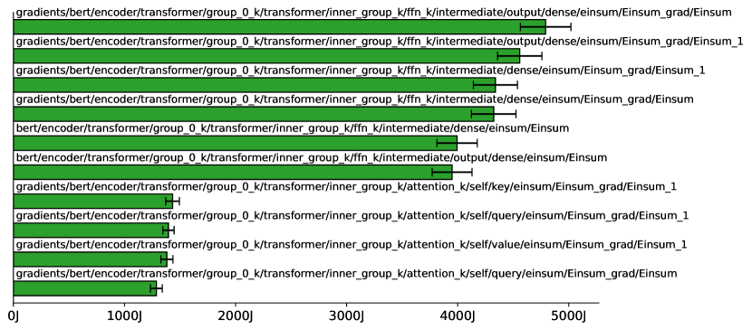
(a) STEF

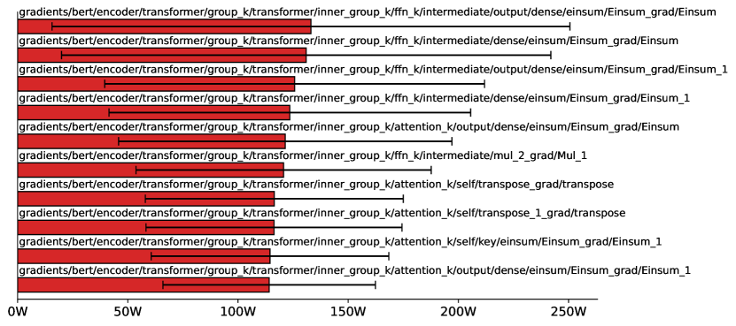
(b) STPF

Figure 10. Top Energy/Power-Consuming Tensors in ALBERT

Fig. 10 presents the STEF and STPF for ALBERT. For all top-10 energy consumers, the EINSUM tensor is used. This refers to Einstein summation, an index-based approach to defining tensor transformations. Indeed, matrix multiplication can also be represented with Einstein summation. From BERT to ALBERT, the transformation has changed from MATMUL to EINSUM, but tensor-based mathematical transformation remains dominant in energy consumption.

ALBERT indeed has some different consumption behavior than BERT. While the distribution of the energy for the STEFs is similar, the values are much smaller, almost half in some cases. In contrast, the STPF of ALBERT shows much higher power consumption — at least 120W — for all of the top-consuming tensors. This indicates that ALBERT is more likely to place GPUs in a higher utilization level. In addition, the standard deviations in power consumption are significantly larger than BERT tensors too. We speculate that it may result from changes in scheduling from BERT to ALBERT. Topologically, BERT chains the transformers in a sequential stack, i.e., the output of the $i^{\tt th}$ transformer is fed into $(i+1)^{\tt th}$ transformer as input. The topology of ALBERT however consists of multiple data pipelines. We think this design change may offer ALBERT more opportunities to execute multiple layers in parallel non-deterministically. This conjecture is also consistent with the fact that GPUs operate at a higher power in ALBERT in BERT.

7. Related Work

Energy Estimation for DL

DeLight (delight2016, ) analytically models the energy cost resulted from forward and backward passes, mathematically captured through the arithmetic operations, activation functions, and propagation errors latent in the DNN. NeuralPower (neuralpower, ) is another analytical approach to estimating the energy consumption of a DNN given its topological details, with a mathematical model to estimate the power consumption and execution time of a DNN inference, together with parameters related to GPU scheduling such as stride size. Energy estimation and energy accounting are fundamentally different problems. While energy estimation offers a priori insight of the DNN energy consumption, energy accounting is conducted a posteriori to answer “what happened.” For energy estimation, a model is assumed, e.g., how propagation and its errors are represented, how computations are kernelized, and how the GPU scheduler sets the stride size. Smaragdine is model-less.

Garcia-Martin et al. (GARCIAMARTIN201975, ) surveyed the energy estimation approaches for ML applications, with a focus on non-DL systems.

Energy Optimization of DL

A direction that received significant interest is the energy optimization of DNNs. Domain-specific architectures and accelerators (tpus, ; lnpu, ) often deliver better energy efficiency. As a well-known example, Tensor Processing Units (TPUs) enable more performance- and energy-efficient executions for applications like TensorFlow. On the algorithm level, there is a long tradition in designing neutral networks with better energy efficiency. For example, SqueezeNext (squeezenext, ) and ChamNet (chamnet, ) considers energy efficiency as a key design constraint. Model compression techniques can often lead to increased energy efficiency, including quantization (jegou2011, ; gong2014, ; Gupta2015DeepLW, ), pruning (LeCun1989OptimalBD, ; han2015deep, ), and distillation (hinton2015distilling, ; huang2017like, ).

Black-box systems-level approaches such as GPOEO (gpoeo, ) and Zeus (zeus285082, ) provide tools to optimize energy consumption on GPUs. For example, Zeus adaptively conducts the training of DNNs with different combinations of batch sizes and GPU power limits, and selects the more energy-optimal configurations on the Pareto curve.

Energy optimization and energy accounting go hand in hand. Smaragdine can complement existing approaches by providing a white-box view on the impact of their energy optimization, describing it in a per-layer or per-tensor manner. § 6 serves as examples to demonstrate how Smaragdine can help designers gain insight on energy optimization, i.e., what has really happened inside a DL program when its energy consumption is reduced/changed.

Modular DL

BERT and ALBERT adopt a modular approach for model construction, whose hierarchical decomposition structure is leveraged by Smaragdine for accounting. DNN modularization is common. For example, Inception (inception1, ; inception2, ) evolves by replacing high-dimension convolutions with a sequence of small ones. Montavon et al.  (montavon2017explaining, ) uses Taylor decomposition of subnetworks to improve network understandability. In addition, there is emerging work in applying modularization to search for sub-networks that were not part of the design specifications  (pan:dnndecomposition, ; kingetsu2021neural, ).

Understanding/Profiling/Debugging DL Programs

TensorFlow has released TensorBoard (tensorflow, ), an API which collects and visualizes key metrics from a DL program runtime. Amazon similarly created the Amazon SageMaker Debugger (sagemaker, ) for real-time monitoring of DL applications. Both of these tools allow designers to compare training and performance metrics. PACE (pace, ) performs accuracy estimation over both the data set and model to identify potential issues before performing full training. Debugging DL programs (mode2018, ; deeplocalize2021, ; autotrainer2021, ; umlaut2021, ; deepfd2022, ) is an important direction in software engineering.

Non-DL Energy Accounting, Profiling, and Modeling

For non-DL applications, energy accounting can be conducted at the levels of hardware (e.g., (icount, )), OS (e.g.,  (currentcy, )), and applications (e.g., (chappie, )). Energy profiling (eprof, ; eandroid, ) and energy modeling (zamani, ; bircher, ; mccullough, ) are established directions in software engineering and computer systems. Their benefits in program understanding and debugging are well known.

8. Threats to Validity

First, our experiments are constructed on systems only with CPUs and GPUs; no additional accelerators are available. Hardware acceleration for DL programs is a rapidly developing field (tpus, ). Our algorithm can be extended to support additional hardware, through extending the energy domains, i.e, the Device construct at Line 6 in Algorithm 1. Second, we rely on RAPL for monitoring CPU power consumption, available primarily on Intel architectures, and on Nvidia-specific interface for monitoring GPU power consumption. This limitation can be overcome through external meters or power modeling (zamani, ; bircher, ). Third, the TensorFlow runtime we currently support is in Python. While this is in sync with the majority of TensorFlow applications (BERT and ALBERT are both developed in Python), we do not have experimental evidence on the effectiveness of TensorFlow energy accounting in other language runtimes. In § 4, we discussed decoupled monitoring, which may facilitate prototyping of our designs for other languages.

9. Conclusion

Tensor-aware energy accounting is a novel methodology where the accounting of energy consumption is aligned with the hierarchical decomposition structure of nested deep neural networks defined in TensorFlow-based deep learning programs. Through energy distribution diagrams and tensor energy footprints, our energy accounting system, Smaragdine is capable of revealing insights on the white-box energy behavior of two widely used natural language models, BERT and ALBERT.

References

- (1) Abadi, M., Barham, P., Chen, J., Chen, Z., Davis, A., Dean, J., Devin, M., Ghemawat, S., Irving, G., Isard, M., Kudlur, M., Levenberg, J., Monga, R., Moore, S., Murray, D. G., Steiner, B., Tucker, P., Vasudevan, V., Warden, P., Wicke, M., Yu, Y., and Zheng, X. Tensorflow: A system for large-scale machine learning. In 12th USENIX Symposium on Operating Systems Design and Implementation (OSDI 16) (Savannah, GA, Nov. 2016), USENIX Association, pp. 265–283.
- (2) Babakol, T., Canino, A., Mahmoud, K., Saxena, R., and Liu, Y. D. Calm energy accounting for multi-threaded java applications. In Proceedings of the 2020 ACM Joint Meeting on European Software Engineering Conference and Symposium on the Foundations of Software Engineering, ESEC/SIGSOFT FSE 2020, Sacramento, CA, USA, November 08-13, 2020.
- (3) Bengio, Y., Ducharme, R., and Vincent, P. A neural probabilistic language model. Advances in neural information processing systems 13 (2000).
- (4) Bircher, W. L., and John, L. K. Complete system power estimation using processor performance events. IEEE Transactions on Computers 61, 4 (2012), 563–577.
- (5) Cai, E., Juan, D.-C., Stamoulis, D., and Marculescu, D. Neuralpower: Predict and deploy energy-efficient convolutional neural networks. 9th Asian Conference on Machine Learning (10 2017).
- (6) Cao, J., Li, M., Chen, X., Wen, M., Tian, Y., Wu, B., and Cheung, S.-C. DeepFD: Automated Fault Diagnosis and Localization for Deep Learning Programs. Association for Computing Machinery, New York, NY, USA, 2022, p. 573–585.
- (7) Chen, J., Wu, Z., Wang, Z., You, H., Zhang, L., and Yan, M. Practical accuracy estimation for efficient deep neural network testing. ACM Trans. Softw. Eng. Methodol. 29, 4 (oct 2020).
- (8) Collobert, R., and Weston, J. A unified architecture for natural language processing: Deep neural networks with multitask learning. In Proceedings of the 25th international conference on Machine learning (2008), pp. 160–167.
- (9) Dai, X., Jia, Y., Vajda, P., Uyttendaele, M., Jha, N. K., Zhang, P., Wu, B., Yin, H., Sun, F., Wang, Y., Dukhan, M., Hu, Y., and Wu, Y. Chamnet: Towards efficient network design through platform-aware model adaptation. In 2019 IEEE/CVF Conference on Computer Vision and Pattern Recognition (CVPR) (Los Alamitos, CA, USA, jun 2019), IEEE Computer Society, pp. 11390–11399.
- (10) Devlin, J., Chang, M.-W., Lee, K., and Toutanova, K. BERT: Pre-training of deep bidirectional transformers for language understanding. In Proceedings of the 2019 Conference of the North American Chapter of the Association for Computational Linguistics: Human Language Technologies, Volume 1 (Long and Short Papers) (Minneapolis, Minnesota, June 2019), Association for Computational Linguistics, pp. 4171–4186.
- (11) Dutta, P., Feldmeier, M., Paradiso, J., and Culler, D. Energy metering for free: Augmenting switching regulators for real-time monitoring. In 2008 International Conference on Information Processing in Sensor Networks (ipsn 2008) (April 2008), pp. 283–294.
- (12) Fukushima, K. Neocognitron: A self-organizing neural network model for a mechanism of pattern recognition unaffected by shift in position. Biological cybernetics 36, 4 (1980), 193–202.
- (13) Gao, X., Liu, D., Liu, D., Wang, H., and Stavrou, A. E-android: A new energy profiling tool for smartphones. In 2017 IEEE 37th International Conference on Distributed Computing Systems (ICDCS) (June 2017), pp. 492–502.
- (14) García-Martín, E., Rodrigues, C. F., Riley, G., and Grahn, H. Estimation of energy consumption in machine learning. Journal of Parallel and Distributed Computing 134 (2019), 75–88.
- (15) Gholami, A., Kwon, K., Wu, B., Tai, Z., Yue, X., Jin, P., Zhao, S., and Keutzer, K. Squeezenext: Hardware-aware neural network design. In Proceedings of the IEEE Conference on Computer Vision and Pattern Recognition (CVPR) Workshops (June 2018).
- (16) Gong, Y., Liu, L., Yang, M., and Bourdev, L. Compressing deep convolutional networks using vector quantization, 12 2014.
- (17) Gupta, S., Agrawal, A., Gopalakrishnan, K., and Narayanan, P. Deep learning with limited numerical precision. In International Conference on Machine Learning (2015).
- (18) Han, S., Mao, H., and Dally, W. J. Deep compression: Compressing deep neural networks with pruning, trained quantization and huffman coding. arXiv preprint arXiv:1510.00149 (2015).
- (19) Hinton, G., Vinyals, O., and Dean, J. Distilling the knowledge in a neural network. arXiv preprint arXiv:1503.02531 (2015).
- (20) Hofmann, K. H. d-1 - the low separation axioms t0 and t1. In Encyclopedia of General Topology, K. P. Hart, J. iti Nagata, J. E. Vaughan, V. V. Fedorchuk, G. Gruenhage, H. J. Junnila, K. M. Kuperberg, J. van Mill, T. Nogura, H. Ohta, A. Okuyama, R. Pol, and S. Watson, Eds. Elsevier, Amsterdam, 2003, pp. 155–157.
- (21) Huang, Z., and Wang, N. Like what you like: Knowledge distill via neuron selectivity transfer. arXiv preprint arXiv:1707.01219 (2017).
- (22) Jouppi, N. P., Young, C., Patil, N., Patterson, D., Agrawal, G., Bajwa, R., Bates, S., Bhatia, S., Boden, N., Borchers, A., Boyle, R., Cantin, P.-l., Chao, C., Clark, C., Coriell, J., Daley, M., Dau, M., Dean, J., Gelb, B., Ghaemmaghami, T. V., Gottipati, R., Gulland, W., Hagmann, R., Ho, C. R., Hogberg, D., Hu, J., Hundt, R., Hurt, D., Ibarz, J., Jaffey, A., Jaworski, A., Kaplan, A., Khaitan, H., Killebrew, D., Koch, A., Kumar, N., Lacy, S., Laudon, J., Law, J., Le, D., Leary, C., Liu, Z., Lucke, K., Lundin, A., MacKean, G., Maggiore, A., Mahony, M., Miller, K., Nagarajan, R., Narayanaswami, R., Ni, R., Nix, K., Norrie, T., Omernick, M., Penukonda, N., Phelps, A., Ross, J., Ross, M., Salek, A., Samadiani, E., Severn, C., Sizikov, G., Snelham, M., Souter, J., Steinberg, D., Swing, A., Tan, M., Thorson, G., Tian, B., Toma, H., Tuttle, E., Vasudevan, V., Walter, R., Wang, W., Wilcox, E., and Yoon, D. H. In-datacenter performance analysis of a tensor processing unit. In Proceedings of the 44th Annual International Symposium on Computer Architecture (New York, NY, USA, 2017), ISCA ’17, Association for Computing Machinery, p. 1–12.
- (23) Jégou, H., Douze, M., and Schmid, C. Product quantization for nearest neighbor search. IEEE Transactions on Pattern Analysis and Machine Intelligence 33, 1 (2011), 117–128.
- (24) Kingetsu, H., Kobayashi, K., and Suzuki, T. Neural network module decomposition and recomposition, 2021.
- (25) Lan, Z., Chen, M., Goodman, S., Gimpel, K., Sharma, P., and Soricut, R. Albert: A lite bert for self-supervised learning of language representations. In International Conference on Learning Representations (2020).
- (26) LeCun, Y., Denker, J. S., and Solla, S. A. Optimal brain damage. In NIPS (1989).
- (27) Lee, J., Lee, J., Han, D., Lee, J., Park, G., and Yoo, H.-J. 7.7 lnpu: A 25.3tflops/w sparse deep-neural-network learning processor with fine-grained mixed precision of fp8-fp16. pp. 142–144.
- (28) Lee, J., Yoon, W., Kim, S., Kim, D., Kim, S., So, C. H., and Kang, J. BioBERT: a pre-trained biomedical language representation model for biomedical text mining. Bioinformatics 36, 4 (09 2019), 1234–1240.
- (29) Linnainmaa, S. Taylor expansion of the accumulated rounding error. BIT Numerical Mathematics 16 (1976), 146–160.
- (30) Ma, S., Liu, Y., Lee, W.-C., Zhang, X., and Grama, A. Mode: Automated neural network model debugging via state differential analysis and input selection. In Proceedings of the 2018 26th ACM Joint Meeting on European Software Engineering Conference and Symposium on the Foundations of Software Engineering (New York, NY, USA, 2018), ESEC/FSE 2018, Association for Computing Machinery, p. 175–186.
- (31) McCullough, J. C., and Agarwal, Y. Evaluating the effectiveness of Model-Based power characterization. In 2011 USENIX Annual Technical Conference (USENIX ATC 11) (Portland, OR, June 2011), USENIX Association.
- (32) Montavon, G., Lapuschkin, S., Binder, A., Samek, W., and Müller, K.-R. Explaining nonlinear classification decisions with deep taylor decomposition. Pattern recognition 65 (2017), 211–222.
- (33) Novikov, A., Podoprikhin, D., Osokin, A., and Vetrov, D. P. Tensorizing neural networks. Advances in neural information processing systems 28 (2015).
- (34) Pan, R., and Rajan, H. On decomposing a deep neural network into modules. In Proceedings of the 28th ACM Joint Meeting on European Software Engineering Conference and Symposium on the Foundations of Software Engineering (New York, NY, USA, 2020), ESEC/FSE 2020, Association for Computing Machinery, p. 889–900.
- (35) Pathak, A., Hu, Y. C., and Zhang, M. Where is the energy spent inside my app?: Fine grained energy accounting on smartphones with eprof. In Proceedings of the 7th ACM European Conference on Computer Systems (2012), EuroSys ’12, pp. 29–42.
- (36) Patterson, D., Gonzalez, J., Le, Q., Liang, C., Munguía, L.-M., Rothchild, D., So, D., Texier, M., and Dean, J. Carbon emissions and large neural network training, 04 2021.
- (37) Rauschmayr, N., Kumar, V., Huilgol, R., Olgiati, A., Bhattacharjee, S., Harish, N., Kannan, V., Lele, A., Acharya, A., Nielsen, J., Ramakrishnan, L., Chandy, I., Bhatt, I., Li, Z., Chia, K., Dodda, N., Gu, J., Choi, M., Nagarajan, B., Geevarghes, J., Davydenko, D., Li, S., Huang, L., Kim, E., Hill, T., and Kenthapadi, K. Amazon sagemaker debugger: A system for real-time insights into machine learning model training. In MLSys 2021 (2021).
- (38) Rob Srebrovic, J. Y. Leveraging the bert algorithm for patents with tensorflow and bigquery. Tech. rep., Global Patents, Google.
- (39) Rouhani, B. D., Mirhoseini, A., and Koushanfar, F. Delight: Adding energy dimension to deep neural networks. In Proceedings of the 2016 International Symposium on Low Power Electronics and Design (New York, NY, USA, 2016), ISLPED ’16, Association for Computing Machinery, p. 112–117.
- (40) Rumelhart, D. E., Hinton, G. E., Williams, R. J., et al. Learning internal representations by error propagation, 1985.
- (41) Schoop, E., Huang, F., and Hartmann, B. Umlaut: Debugging deep learning programs using program structure and model behavior. In Proceedings of the 2021 CHI Conference on Human Factors in Computing Systems (New York, NY, USA, 2021), CHI ’21, Association for Computing Machinery.
- (42) Strubell, E., Ganesh, A., and McCallum, A. Energy and policy considerations for deep learning in NLP. CoRR abs/1906.02243 (2019).
- (43) Szegedy, C., Liu, W., Jia, Y., Sermanet, P., Reed, S., Anguelov, D., Erhan, D., Vanhoucke, V., and Rabinovich, A. Going deeper with convolutions. In Computer Vision and Pattern Recognition (CVPR) (2015).
- (44) Szegedy, C., Vanhoucke, V., Ioffe, S., Shlens, J., and Wojna, Z. Rethinking the inception architecture for computer vision. In 2016 IEEE Conference on Computer Vision and Pattern Recognition (CVPR) (2016), pp. 2818–2826.
- (45) US-NSF. National science foundation and vmware partnership on the next generation of sustainable digital infrastructure (ngsdi), nsf 20-594, 2020.
- (46) Vaswani, A., Shazeer, N., Parmar, N., Uszkoreit, J., Jones, L., Gomez, A. N., Kaiser, L., and Polosukhin, I. Attention is all you need. In Proceedings of the 31st International Conference on Neural Information Processing Systems (Red Hook, NY, USA, 2017), NIPS’17, Curran Associates Inc., p. 6000–6010.
- (47) Wang, F., Zhang, W., Lai, S., Hao, M., and Wang, Z. Dynamic gpu energy optimization for machine learning training workloads. IEEE Transactions on Parallel I& Distributed Systems 33, 11 (nov 2022), 2943–2954.
- (48) Wardat, M., Le, W., and Rajan, H. Deeplocalize: Fault localization for deep neural networks. In Proceedings of the 43rd International Conference on Software Engineering (2021), ICSE ’21, IEEE Press, p. 251–262.
- (49) Warstadt, A., Singh, A., and Bowman, S. R. Neural network acceptability judgments. arXiv preprint arXiv:1805.12471 (2018).
- (50) You, J., Chung, J.-W., and Chowdhury, M. Zeus: Understanding and optimizing GPU energy consumption of DNN training. In 20th USENIX Symposium on Networked Systems Design and Implementation (NSDI 23) (Boston, MA, Apr. 2023), USENIX Association, pp. 119–139.
- (51) Zamani, R., and Afsahi, A. A study of hardware performance monitoring counter selection in power modeling of computing systems. In 2012 International Green Computing Conference (IGCC) (2012), pp. 1–10.
- (52) Zeng, H., Ellis, C. S., Lebeck, A. R., and Vahdat, A. Ecosystem: managing energy as a first class operating system resource. In ASPLOS-X: Proceedings of the 10th international conference on Architectural support for programming languages and operating systems (2002), pp. 123–132.
- (53) Zeng, H., Ellis, C. S., Lebeck, A. R., and Vahdat, A. Currentcy: A unifying abstraction for expressing energy management policies. In In Proceedings of the USENIX Annual Technical Conference (2003), pp. 43–56.
- (54) Zhang, X., Zhai, J., Ma, S., and Shen, C. Autotrainer: An automatic dnn training problem detection and repair system. In 2021 IEEE/ACM 43rd International Conference on Software Engineering (ICSE) (2021), pp. 359–371.