Precision at the indistinguishability threshold: a method for evaluating classification algorithms

Abstract

There exist a wide range of single number metrics for assessing performance of classification algorithms, including AUC and the F1-score (Wikipedia lists 17 such metrics, with 27 different names). In this article, I propose a new metric to answer the following question: when an algorithm is tuned so that it can no longer distinguish labelled cats from real cats, how often does a randomly chosen image that has been labelled as containing a cat actually contain a cat? The steps to construct this metric are as follows. First, we set a threshold score such that when the algorithm is shown two randomly-chosen images — one that has a score greater than the threshold (i.e. a picture labelled as containing a cat) and another from those pictures that really does contain a cat— the probability that the image with the highest score is the one chosen from the set of real cat images is 50%. At this decision threshold, the set of positively labelled images are indistinguishable from the set of images which are positive. Then, as a second step, we measure performance by asking how often a randomly chosen picture from those labelled as containing a cat actually contains a cat. This metric can be thought of as precision at the indistinguishability threshold. While this new metric doesn’t address the tradeoff between precision and recall inherent to all such metrics, I do show why this method avoids pitfalls that can occur when using, for example AUC, and it is better motivated than, for example, the F1-score.

1 Introduction

Imagine you have created an algorithm (a machine learning model) that assigns a score, predicting whether an entity belongs to one of two classes (positive and negative). For example, the input might be a picture and the output whether or not the picture contains a cat. The scores are larger if your algorithm evaluates the object as more likely to belong to the positive class (i.e if it labels the image as more likely to contain a cat). Such a scoring system explicitly underlies, for example, logistic regression, the output of a neural network and discriminant analysis [1]. Other, non-parametric machine learning methods, such as $k$-nearest neighbours [2], don’t have an explicit score, but often have a parameter (e.g. $k$) which can be tuned in a way that mimics a threshold.

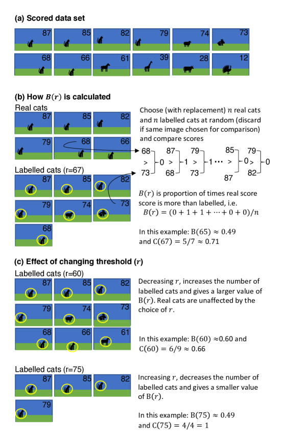
Figure 1: Illustration of the method described in this paper

The method I suggest for evaluating performance in this article is as follows. We start, in figure 1a, with a data set in which every image is assigned a score. We first investigate what happens when we set a threshold score, $r$, above which we label the image as containing a cat (positive), below which we label the image as not containing a cat (negative). For any given threshold we compare those images which we label as cats (given the threshold) with those containing real cats. Specifically, we choose (with replacement) $n$ real cats and $n$ labelled cats at random and compare scores (figure 1b). In cases where we happen to pick the same two images, we pick two new images for that particular comparison. This gives a measure $B(r)$: the probability a real cat scores more than a labelled cat for threshold $r$.

We then identify a specific threshold score, $r_{b}$, such that if we were to choose one image that the algorithm classifies as containing a cat and a second image that really does contain a cat, then the probability that the score of the image containing the cat is the largest of the two scores is 50%. We define this as $r_{b}$, where $B(r_{b})\approx 0.5$. In the example, in figure 1b $r_{b}=67$. A smaller threshold gives $B(r_{b})>0.5$ and a larger threshold gives $B(r_{b})<0.5$ (figure 1c). We call $r_{b}$ the indistinguishability threshold: because the set comprised of false positives (FP) and true positives (TP) is indistinguishable from the set of TPs and true negatives (TN). When $r=r_{b}$, if we pick (at random) two images from our data set, one which is labelled as a cat and the other that is known to contain a cat, then the probability that the algorithm will score assign the image with the cat the highest score is one half.

To measure the performance of your algorithm, simply calculate the proportion of images the algorithm classifies as containing a cat do actually contain a cat. I denote this measure $C(r_{b})$ and call it precision at the indistinguishability threshold.

There already exist a number of ways of evaluating classification algorithms. Wikipedia lists a somewhat bewildering array of 17 tests, with a total of 27 different names, for such problems. The most commonly used method is the area under the Receiver-Operator Curve, commonly referred to as AUC [3, 4, 5]. Another popular choice is the F1-score [6], which seeks to avoid a problem inherent in AUC when applied to unbalanced data [1]. In this paper, I argue that $C(r_{b})$ provides an easy to understand alternative to F1-score, which avoids many of the problems inherent to AUC.

2 Data set

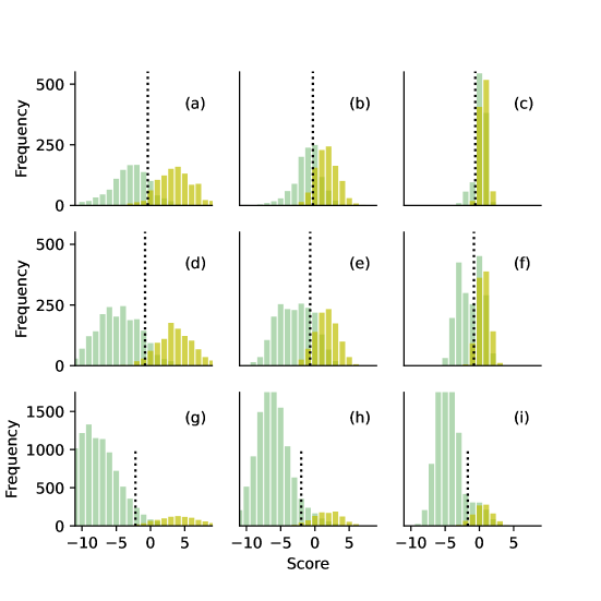
Figure 2: The score distributions for the nine example data sets we look at here. Green are members of the negative class, yellow members of the positive class. The dotted line shows $r_{b}$, the solution $B(r)=1/2$ (see equation 6)

I use nine artificial data sets, as shown in figure 2. The positive class ($Y_{i}=1$) is created by first generating 1000 input values, $X_{i}$, with a mean $m_{p}=10$ and standard deviation $\sigma_{p}=2$. Similarly, the negative class ($Y_{i}=-1$) consists of 1000 ‘difficult’ data points with values, $X_{i}$, which have mean scores (a,d,g) $m_{n}=5$; (b,e,h) $m_{n}=7$; (c,f,i) $m_{n}=9$ and (in all cases) standard deviation $\sigma_{n}=2$, along with (a,b,c) 10000; (d,e,f) 1000; (d,e,f) 100 ‘easy’ data points, $X_{i}$, with mean 2 and standard deviation 2. I then performed logistic regression on $X_{i}$ to predict $Y_{i}$ and calculated the log-likelihood for every individual point. These log-likelihoods are taken to be the scores, $S_{i}$, output by the model and are plotted in figure 2.

The choice of these data sets is to give a range of difficulty levels. The data in the left column correspond to relatively easy classification tasks. The overlap between the green (negative) and yellow (positive) is small. The data in the right column is much more difficult, with a large overlap in scores for negative and positive. The datasets at the bottom include a large number of ‘easy’ to classify negative values, but the size of the overlap is only slightly increased over the datasets at the top. The data generation method and the code are available at: https://github.com/soccermatics/ABC.git.

3 Results

3.1 Area under the curve

Let’s start by asking the following question about our data: how often does a member of the positive class score higher than a member of the negative class?

To measure this we pick one member of the positive class at random and one member of the negative class at random and we will look to see which of them has the highest score. As a concrete example, imagine an algorithm is shown two images, one which contains a cat, another which does not. The task is to pick the image containing the cat. We call this probability

$$A=P(S_{P}>S_{N})$$

where $S_{P}$ is the score of a randomly chosen positive member and $S_{N}$ is the score of a randomly chosen negative member. The value of $A$ can be measured directly, simply by randomly picking pairs of members of negative and positive classes and testing which scores higher. The test outcome is then the proportion of cases in which the positive member receives a higher value than the negative member.

We can also measure the paired comparison test over all our scores. Let $F_{P}(r)$ be the cumulative distribution of scores of the positive class, i.e.

$$F_{P}(r)=P(S_{P}<r)=\int_{s=-\infty}^{r}f_{P}(s)ds$$ (1)

where $f_{P}(r)$ is thus the probability density function of $S_{P}$. Likewise, we let $F_{N}(r)$ to be the cumulative distribution of scores the negative class, i.e.

$$F_{N}(r)=P(S_{N}<r)=\int_{s=-\infty}^{r}f_{N}(s)ds$$ (2)

The value $A=P(S_{P}>S_{N})$, can be written as the conditional probability distribution

$$A=\int_{r=-\infty}^{\infty}\int_{s=r}^{\infty}f_{N}(r)\cdot f_{P}(s)dsdr$$ (3)

which is equivalent to

$$A=\int_{r=-\infty}^{\infty}f_{N}(r)\int_{s=r}^{\infty}f_{P}(s)dsdr=\int_{r=-\infty}^{\infty}f_{N}(r)\cdot\left(1-F_{P}(r)\right)dr$$ (4)

We can use this equation to calculate $A$ by numerical integration.

More importantly, we can also use this formulation to note an equivalence between the $A$ test above and another commonly used measure of accuracy, namely, AUC (the area under the ROC/receiver operator curve). ROC curves plot the false positive rate against the true positive rate, as parametrised curves of $r$. Note that the true positive rate for a given threshold $r$ is given by $v(r)=1-F_{P}(r)$ and that the false positive rate for a given threshold $r$, is given by $u(r)=1-F_{N}(r)$. Then we see that

$$A=\int_{r=-\infty}^{\infty}v(r)f_{N}(r)dr$$

which by change of variable gives

$$A=\int_{u=0}^{1}v\left(u^{-1}(r)\right)du$$ (5)

where $u^{-1}(r)$ denotes the inverse of $u(r)$. Thus $A$ is also the area under the ROC curve (which is defined by the right hand side of equation 5).

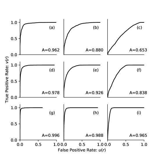
Figure 3: The area under the curve for each of the scores in figure 2

The ROC curves are shown in figure 3 for our nine data sets. The area under these curves (i.e. $A$) is shown as text within the figure. The value of $A$ is close to one when either the scores for the negative and positive class are typically different (e.g. for the score distributions shown in figure 2 a, d and g) or there are a large proportion of ’easy’ to score negative members (e.g. for the score distributions shown in figure 2 h and i).

These examples illustrate both the power and the limitation of $A$ as a measure. In the cases a, d and g – where the score accurately distinguishes class members – $A$ reflects the fact it is more likely that the algorithm picks out the positive cases correctly. But in the cases where there is an overlap between the positive and ’difficult’ negative class (e.g. cases c, h and i) we see that as we add more ’easy’ cases (i.e. go from c through f to i) the accuracy of the model appears to increase, despite the fact that the difficult cases are equally difficult in all three data sets. We could see this as giving a possibility for ‘cheating’: by adding more easier cases to our data set we can appear to be improving accuracy, as measured by $A$, while no such improvement is actually occurring.

This is why we need to be very clear about what the AUC test tells us: it tells us that if we pick one member of the positive class at random it has probability $A$ of having a higher score than one member of the negative class chosen at random. When there are a lot more ’easy’ to classify members of the negative class then a high value of $A$ is not surprising: most of the time we will randomly pick one of those members. Thus in figure 3i an $A$ close to one tells us very little about how well our algorithm can distinguish more difficult cases.

3.2 Indistinguishability threshold

We now look at how often a member of the positive class scored higher than a member that has been labelled positive. To do this, we pick a random member of the positive class and we compare its score to the score of a random individual that has been labelled (predicted) positive. For example, in the cat labelling problem, we first pick randomly from all images containing cats and denote the score of this image as $S_{P}$. Then, for a given threshold $r$, we choose randomly from all the images with that score or above, irrespective of whether or not they contain a cat. We denote this score of this image as $S_{R}$. We then calculate the probability

$$B(r)=P(S_{P}>S_{R}|S_{R}>r)$$

or, in words, the probability that a random member of the positive class scores higher than a random member of the class we have labelled as positive (i.e. has a score greater than $r$).

Unlike the paired comparison of negatives and positives we made in the previous section, it is not immediately clear how this test will help us construct a performance metric. To gain some more intuition, let’s think about what happens as we change the threshold $r$. When $r$ is very large then the positively labelled set will contain more positives than negatives, but very few members of either class. As a result $P(S_{P}>S_{R}|S_{R}>r)$ will go towards $0$. When $r$ is small (or negative), most images are labelled positive. Nearly all members of the positive class will be included in the positively labelled set, but so too will most members of the negative class. Neither of these two situations is desirable. In the former, we will have a lot of false positive errors and very low precision (or sensitivity): a high proportion of those labelled positive will actually be negative. In the latter case, we will have a large proportion of false negatives but very high precision: most of those which are labelled positive are actually positive.

I suggest choosing $r_{b}$ such that

$$B(r_{b})=P(S_{P}>S_{R}|S_{R}>r_{b})=1/2$$ (6)

because this particular value of $r_{b}$ has a rather desirable property. It means that, as far as the classifier is concerned the images in the positive class are indistinguishable from those which we have labelled positive. If we pick a random member of the images we have classified as positive and a random member of the positives, these two images are equally likely to be classified as positive. We can thus think of $r_{b}$ as being the threshold value at which the model cannot distinguish between true positives and labelled positives. The algorithm cannot distinguish reality from its own labelling. We thus refer to $r_{b}$ as the indistinguishability threshold.

To understand why this is desirable, think about a situation where we have two separate test sets of images, $Y_{1}$ and $Y_{2}$, and we want to check whether or not they have a similar distribution of scores. A solution to this problem might be to pick members from both $Y_{1}$ and $Y_{2}$ at random and compare their scores. If roughly half of the time members of $Y_{1}$ scored higher than members of $Y_{2}$ we might say that the two groups are indistinguishable. In the same way, by setting $r_{b}$ using equation 6, we are finding a threshold so that the positive class is indistinguishable from the set that is labelled positive. The vertical dotted lines in figure 2 shows the value of $r_{b}$ for our nine example score distribution sets. For all nine distributions the lines give a reasonable separation between the scores, lying roughly halfway between the ‘difficult’ negative cases and the positive cases.

A common (but misguided) alternative to choosing $r=r_{b}$ is to instead choose $r$ such that

$$P(S_{P}=r)=1-P(S_{P}=r)$$ (7)

or, equivalently,

$$P(S_{P}=r)=1/2$$ (8)

where we define an underlying model which converts scores in to probabilities. For example, when the scores have been estimated by logistic regression then a natural choice is the logistic function

$$P(S_{P}=r)=\frac{1}{1+\exp(r)}=1/2$$

which gives $r=0$ as the threshold. Looking again at the distribution of scores in figure 2 we see that the size of the negative class shifts the distribution of the scores generated by the logistic regression to the right. This is undesirable, because it means that the algorithm will make more errors when easy to categorise cases are added to the data set.

The limitations of using equation 8 to set a threshold are known, but often they are referred to as being “caused by an unbalanced data set”. The implication is that too many members in the negative class have somehow misled us in to choosing a poor value of $r$. In my experience, students and even experienced practitioners, when confronted with this problem, either start to prune their data, removing ‘easy’ members of the negative class, or oversample from the positive class in order to compensate. They might also draw an ROC curve and a Precision-Recall curve (see below) and try to justify, in an ad-hoc fashion, choosing a different value of the threshold $r$ on the basis of what they see in these curves.

It is not the data set that is imbalanced. It is rather our way of looking at it that is wrong! Specifically, it is the arbitrary choice of $r=0$ that is imbalanced.

While both of the two measures — $A$ and $B(r)$ — that we have looked at so far have sensible, method independent interpretations that give us a measure performance, this is not the case for equation 7, which is simply the score for which the probability of receiving a positive label equals that of receiving a negative label. In logistic regression, the model is adjusting to account for the fact that negative cases are more likely than positive cases: negative cases are the more likely outcome and it requires more evidence to persuade us otherwise. But in an application where, for example, we are scanning for a medical condition, the number of negatives (be it 90% or 99.99999% of the population) should not influence how we decide that a case is likely to be positive.

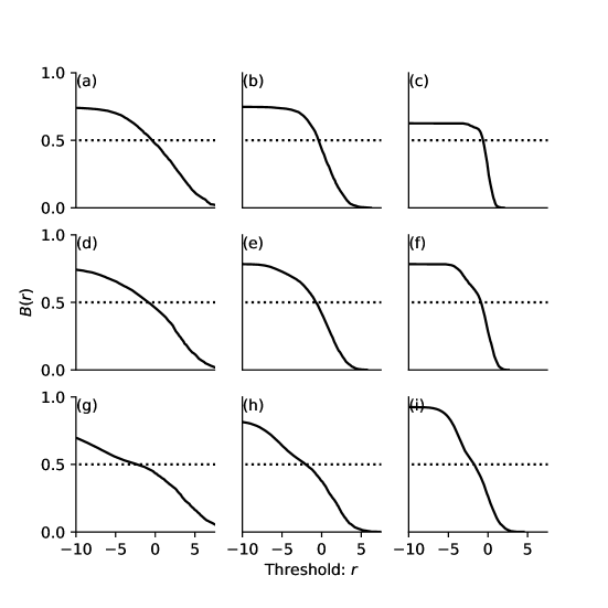
Figure 4: Plot of $B(r)$ for our 9 example data sets. The dotted line is at $1/2$ indicates the value at which the model is balanced.

Neither $r_{b}$ nor $B(r)$ provide a measure of model performance, like $A$ does. Instead they are both measurements around which we can organise a rigorous evaluation of our model. We will look at how $B(r)$ can be used to construct such a measure in section 3.4. In this next section, which can be skipped by readers who just want to know about the performance measure, we look at some properties of $B(r)$.

3.3 Properties and implementation of $B(r)$

As with $A$ the pairwise nature of the test means it is straightforward to implement a randomised version of $B(r)$. For each value of $r$ we sample, with or without replacement, $n$ members of the positive class. Then we sample $n$ members from the set labelled positive when the threshold is greater than $r$. Pairwise comparison of the scores of these two sets gives $B(r)$ . This method becomes less reliable for large values of $r$, since the size of the positive labelled class becomes small and all the comparisons will be made to a small number of positively labelled images.

Another way to calculate $B(r)$, following the AUC approach to estimating $A$, is by integration over the true positive rate, $y(r)$, and the false positive rate, $x(r)$. We now derive the appropriate integral. First, let $S_{R}$ be the score of a randomly chosen positive member. The probability the members has a score less than a randomly chosen member of the positive class with a score greater than $r$ is then written as $P(S_{R}<S_{P}|S_{R}>r)$. It is this probability we call $B(r)$.

Our approach to finding an expression for $B(r)$ is to look separately at the case where $S_{R}$ is from a negative member and a positive member. We can use the law of total probability to give

$$B(r) = P(S_{R}<S_{P}|S_{R}>r)$$ (9)

$$= P(S_{R}<S_{P}|S_{R}>r,R=+)\cdot P(R=+|S_{R}>r)$$

$$+P(S_{R}<S_{P}|S_{R}>r,R=-)\cdot P(R=-|S_{R}>r)$$

where $+$ and $-$ are respectively the events that the chosen individuals are in the positive and negative classes. If an individual is chosen at random then

$$P(R=+|S_{R}>r)=\frac{Pv(r)}{Nv(r)+Pu(r)}\mbox{ and }P(R=-|S_{R}>r)=\frac{Nu(r)}{Nv(r)+Pu(r)}$$ (10)

Furthermore,

$$P(S_{R}<S_{P}|S_{R}>r,R=+) = \frac{P(S_{R}<S_{P}\cap S_{R}>r,R=+)}{P(S_{R}>r,R=+)}$$ (11)

$$= \frac{\int_{t=r}^{\infty}\int_{s=t}^{\infty}f_{P}(t)f_{P}(s)dt}{\int_{t=r}^{\infty}f_{P}(t)dsdt}$$

$$= \frac{\int_{t=r}^{\infty}f_{P}(t)v(t)dt}{v(r)}$$

Since the derivative of $v(r)$ is equal to $-f_{P}(t)$ we can change variable to $v$ in the integral in the numerator to get

$$\int_{t=r}^{\infty}f_{P}(t)v(t)dt=\int_{t=r}^{\infty}v(t)\left(-v^{\prime}(t)\right)dt=\int_{v(r)}^{\infty}v(t)dv=\frac{v(r)^{2}}{2}$$ (12)

and thus simplify to get

$$P(S_{R}<S_{P}|S_{R}>r,R=+)=\frac{v(r)}{2}$$ (13)

We can follow similar steps for the case that $R$ is negative to get,

$$P(S_{R}<S_{P}|S_{R}>r,R=-)=\frac{\int_{t=r}^{\infty}f_{N}(t)u(t)dt}{u(r)}$$ (14)

Substituting 10, 13 and 14 in to equation 9 gives

$$B(r)=\frac{Pv(r)^{2}/2+N\int_{t=r}^{\infty}f_{N}(t)u(t)dt}{Nv(r)+Pu(r)}$$ (15)

This equation is plotted as the black line in figure 4. We see that it goes towards a maximum when $r\rightarrow-\infty$, taking the value

$$B(-\infty)=\frac{P/2+NA}{N+P}$$

and decreases to zero as $r$ increases, so that $B(\infty)=0$. The value $r_{b}$, the solution $B(r_{b})=1/2$, is identified as the point in figure 4 where $B(r)$ crosses the dotted line at $1/2$. This is also the value of $r_{b}$ plotted as the dotted line in figure 4. We will look in more detail at the function $B(r)$ in more detail in section 3.6 and compare it to other measures.

3.4 Precision at the indistinguishability threshold

How often is our positive labelling correct when reality and labelling are indistinguishable? To answer this question, we define $C(r)$ to be the precision: the probability that an individual with a score greater than $r$ is in the positive class, i.e. $P(R=+|S_{R}>r)$ , or the probability that a positive labelling is made correctly. Using Bayes law, we can rewrite precision in terms of false positive rate and true positive rate. Specifically,

$$C(r) = P(R=+|S_{R}>r)$$

$$= \frac{P(S_{+}>r|R=+)P(C=+)}{P(S_{+}>r|R=+)P(R=+)+P(S_{-}>r|R=-)P(R=-)}$$

In this case, $P(R=+)=P/(P+N)$ is the proportion of individuals in the positive class and $P(R=-)=N/(P+N)$ is proportion in the negative class. Substituting $v(r)=P(S_{+}>r|R=+)$ (true positive rate) and $u(r)=P(S_{-}>r|R=-)$ (false positive rate) gives

$$C(r)=\frac{Pv(r)}{Pv(r)+Nu(r)}$$ (16)

When $N$ is much larger than $P$ then $v(r)$ has to be significantly larger than $u(r)$ for precision to have a large value. It is the ratio of true positives, $v(r)$, to all positives, $v(r)$ and $u(r)$, weighted by the frequency at which individuals are, respectively, positive and negative.

I propose measuring precision specifically with a value of $r=r_{b}$, i.e. for a threshold whereby data classified as positive cannot be distinguished from data which truly is positive, i.e. we calculate $C(r_{b})$. Evaluating this for the data in figure 2 (a), (d) and (g) we get $C(r_{b})\approx 0.85$. This could be considered a reasonably good performance: 85% of the pictures the algorithm says are cats are in fact cats. For figure 2 (b), (e) and (h) we get $C(r_{b})\approx 0.69$. This is not a great performance, but could be useable in certain applications: 69% of the pictures the algorithm says are cats are in fact cats. Finally, for the data in figure 2 5 (c), (f) and (i) we get $C(r_{b})\approx 0.50$. This is poor performance, and is probably not very useful in most applications: only 50% of the pictures the algorithm says are cats are in fact cats.

We can now see why $C(r_{b})$ is preferable measure of performance over $A$. When we calculated $A$, the value was highly dependent on the number of ‘easy’ cases. This is not the case with $C(r_{b})$. By evaluating precision when the algorithm cannot distinguish reality from its own labelling, we obtain a measure of performance that doesn’t depend on the number of ‘easy’ cases. The choice of $r_{b}$ is theoretically motivated (in the previous section) and gives reasonable results. In section 3.6 we will compare $C(r_{b})$ to other known metrics for measuring performance, but before we do this, we look at how we might be flexible about our choice of $r$.

3.5 Tuning false positive and true positive rates

There are two further questions we might ask.

1. How often is a member of the positive class detected by the test? This is the true positive rate, $v(r)$.

2. How often is a member of the negative class labelled positive by the test? This is the false positive rate, $u(r)$.

Typically, one of these rates will be more important than another. For example, we might, in a medical screening task, accept a higher false positive rate in order to make sure all those who are positive for a condition are identified. In this case we set $r$ to be a smaller value so as to get a high true positive rate, but also (possibly) a high false positive rate. In a targeted advertising task, where people who might be interested in a product should be identified, we might concentrate on having a lower false positive rate and accept a lower true positive rate, identifying only individuals who are very likely to be interested in the advertised product. In this case we set $r$ to a larger value. In general, there is no escaping from the fact that the measure of performance, and thus the choice of $r$, is informed by the application area.

An alternative here is to set an acceptable range for having a threshold which does not preserve the property that reality is indistinguishable from labelling. A rule of thumb is 40/60. If, for example, we want to ensure a high level of true positives, we find $r_{60}$ by solving $B(r_{60})=0.6$, so that the probability a member classified as positive has a lower score than a truly positive member is 60%. This is shown as the dotted lines in figure 5 to the right of the solid line (at which $B(r_{b})=1/2$). Similarly, we can find $r_{40}$ by solving $B(r_{40})=0.4$, which is given to the left. Note that, while $B(r_{60})>B(r_{b})>B(r_{40})$, the thresholds have the relationship $r_{60}<r_{b}<r_{40}$. A lower threshold leads to more true positives and more false positives.

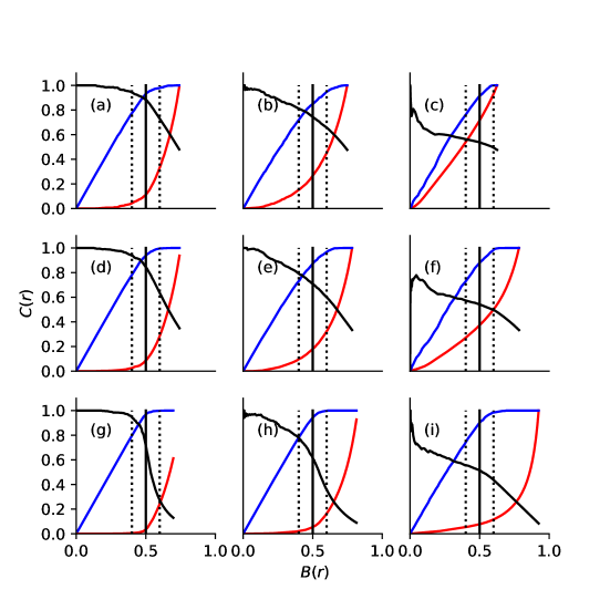
Figure 5: Plot of $B(r)$ against the precision $C(r)$ (black line), true positive rate $v(r)$ (blue) and false positive rate $u(r)$ (red) for our 9 example data sets. These curves are parameterised by $r$.

Figure 5 shows $C(r)$ (black line) plotted against $r$ for our nine test data sets. Again, the way we built $B(r)$ allows us to explain in words what we are doing here. We can, for example, write about figure 5(e) that, "accepting a 60/40 imbalance in favour of positives our algorithm’s predictions in favour of the positive class gave us a precision of $C(r_{60})=0.59$, compared to $C(r_{b})=0.72$ at 50/50 balanced predictions."

3.6 Similarity to F1 score

This section is a few notes about how $B(r)$ relates to some other measures of performance. To do this, I first break equation $B(r)$ in to two components,

$$B(r)=B_{+}(r)+B_{-}(r)$$ (17)

such that

$$B_{+}(r)=\frac{Pv(r)^{2}/2}{Nv(r)+Pu(r)}=\frac{1}{2}v(r)C(r)$$ (18)

and

$$B_{-}(r)=\frac{N\int_{t=r}^{\infty}f_{N}(t)u(t)dt}{Nv(r)+Pu(r)}$$ (19)

These terms are plotted in figure 6. We now look at these two terms individually.

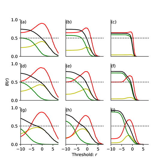
Figure 6: Plot of $B(r)$ for our 9 example data sets. The black line is $B(r)$. The dotted line at $1/2$ indicates the value at which the model is balanced. The yellow line is the component $B_{+}(r)$ (equation 18) and the green line is $B_{-}(r)$ (equation 19). The red line is the $F_{1}(r)$ score (equation 20).

Equation $B_{+}(r)$ is the recall multiplied by the true positive rate, divided by two. This is related to the the F1-score which is defined as,

$$F_{1}(r)=\frac{2C(r)v(r)}{C(r)+v(r)}$$ (20)

In figure 6 we see that $F_{1}$ reaches a maximum at roughly the same point as which $B_{+}(r)$ is maximized. Figure 6 shows that (with the exception of 6 g) the F1 score reaches a maximum at roughly the same point that $B(r)=1/2$. I have not derived the exact form of this relationship and it would be interesting to look at this in more detail, since F1 is seen as a standard test of model performance.

The measure $B_{-}(r)$ is similar to the integral which gives the area under the Precision-Recall curve, which is

$$\int_{s=-\infty}^{\infty}C(t)f_{N}(t)dt\int_{s=-\infty}^{\infty}\frac{Pv(t)}{Pv(t)+Nu(t)}f_{N}(t)dt$$

The difference to $B_{-}(r)$, is that the integral includes the denominator. The term for $B_{-}(r)$ can also be thought of as a sort of $A(r)$, an AUC for those values with scores greater than $r$. Again, this needs to be looked at in more detail.

4 Conclusions

The first test in this article, $A$, —how often is a randomly chosen member of the positive class scored higher than randomly chosen member of the negative class?—is equivalent to calculating the AUC. In many applications, discerning between pairs of negative and positive cases might not be the most important challenge. Clinicians, for example, aren’t usually presented with two people, one of whom they know is sick and one who is healthy, and asked to find the sick individual! Emphasising that $A$ answers a specific question about paired comparison makes its limitation clear: knowing $A$ tells us about paired comparisons between scores. It does not answer all questions we might have about the accuracy of our approach.

The second test, $B(r)$, doesn’t, by itself, tell us about algorithm performance. It instead provides a principled way of deciding on the threshold, $r_{b}$ such that $B(r_{b})=1/2$, to choose for a decision. We tune our threshold, so that the set of pictures the algorithm labels as containing cats is indistinguishable from those which really do contain cats. In addition to laying the basis for our next test, one potentially useful application of this idea would be in boosting [7]. If we fit a model first on all images, then we fit a new model on precisely the images with scores greater than $r_{b}$ then we may be able to iteratively improve the model fit.

The third test, $C(r_{b})$, is the one I recommend for performance. We look at how often the positive labelling is correct when reality and labelling by the algorithm are indistinguishable. All tests of performance have a degree of arbitrariness, but the advantage of this one is that the threshold for the model is that the threshold is set on a single principle: that of indistinguishability. In our examples, this method avoided the limitations of $A$, where the addition of too many ’easy’ cases inflated the area under the curve. Test $C(r_{b})$ answers the following question: when the algorithm is tuned so that it can no longer distinguish labelled cats from real cats, how often is a randomly chosen member that is labelled positive actually a member of the positive class? A more technical short hand for this might be, precision at the indistinguishability threshold.

A valid critique of the method outlined here is that there is no such thing as a single metric for measuring model performance. This point has been recognised since Neyman and Pearson’s showed that for tests of statistical hypotheses there is always a trade-off between two possible error types (false positives and false negatives) [8, 9]. The necessity of this tradeoff means that any single metric (including AUC, F1 and precision at the indistinguishability threshold) cannot claim generality. This limitation has the potential to lead to problems, especially in medical applications [3], where costs and benefits should be assigned to the two error types and the algorithm should be assessed in light of this choice [10, 11].

That said, the development of many machine learning algorithms occurs in a way that is decoupled from particular applications and, as such, the tradeoffs between error types has not yet been specified. This article has argued that, in such situations, precision at the indistinguishability threshold combines the respective advantages of AUC – that it can be explained simply in words – and F1– it does not inflate performance for unbalanced data sets – in a single metric. I would thus encourage researchers to use $C(r_{b}$ instead of just reporting AUC or F1 in settings where error type trade-offs have yet to be specified.

5 Acknowledgements

Thanks to Daniel Gedon and Andre Teixeira for feedback.

References

- [1] A. Lindholm, N. Wahlström, F. Lindsten, and T. B. Schön, Machine Learning - A First Course for Engineers and Scientists. Cambridge University Press, 2022.
- [2] E. Fix and J. L. Hodges, “Discriminatory analysis. nonparametric discrimination: Consistency properties,” International Statistical Review/Revue Internationale de Statistique, vol. 57, no. 3, pp. 238–247, 1989.
- [3] N. A. Obuchowski and J. A. Bullen, “Receiver operating characteristic (roc) curves: review of methods with applications in diagnostic medicine,” Physics in Medicine & Biology, vol. 63, no. 7, p. 07TR01, 2018.
- [4] S. Vanderlooy and E. Hüllermeier, “A critical analysis of variants of the auc,” Machine Learning, vol. 72, pp. 247–262, 2008.
- [5] M. Majnik and Z. Bosnić, “Roc analysis of classifiers in machine learning: A survey,” Intelligent data analysis, vol. 17, no. 3, pp. 531–558, 2013.
- [6] Y. Sasaki et al., “The truth of the f-measure,” Teach tutor mater, vol. 1, no. 5, pp. 1–5, 2007.
- [7] R. E. Schapire, “The boosting approach to machine learning: An overview,” Nonlinear estimation and classification, pp. 149–171, 2003.
- [8] J. Neyman and E. S. Pearson, “Ix. on the problem of the most efficient tests of statistical hypotheses,” Philosophical Transactions of the Royal Society of London. Series A, Containing Papers of a Mathematical or Physical Character, vol. 231, no. 694-706, pp. 289–337, 1933.
- [9] C. Scott, “Performance measures for neyman–pearson classification,” IEEE Transactions on Information Theory, vol. 53, no. 8, pp. 2852–2863, 2007.
- [10] K. Chu, “An introduction to sensitivity, specificity, predictive values and likelihood ratios,” Emergency Medicine, vol. 11, no. 3, pp. 175–181, 1999.
- [11] A. Care, F. A. Ramponi, and M. C. Campi, “A new classification algorithm with guaranteed sensitivity and specificity for medical applications,” IEEE Control Systems Letters, vol. 2, no. 3, pp. 393–398, 2018.