Massive spin-flip excitations in a $\nu\!=\!2$ quantum Hall ferromagnet

Abstract

Excitation with a massive spin reversal of the individual skyrmion/antiskyrmion type is theoretically studied in a quantum Hall ferromagnet, where the zero and first Landau levels are completely occupied only by electrons with spins aligned strictly in the direction determined by the magnetic field. The Wigner-Seitz parameter is not necessarily considered to be small. The microscopic model in use is based on a reduced basic set of quantum states [the so-called “single-mode (single-exciton) approximation”], which allows proper account to be taken for mixing of Landau levels, and substantiating the equations of the classical $O(3)$ nonlinear $\sigma$ model. The calculated ‘spin stiffness’ determines the exchange gap for creating a pair of skyrmion and antiskyrmion. This gap is significantly smaller than the doubled cyclotron energy and the characteristic electron-electron correlation energy. Besides, the skyrmion–antiskyrmion creation gap is much smaller than the energy of creation of a separated electron–exchange-hole pair calculated in the limit case of a spin magnetoexciton corresponding to an infinitely large 2D momentum. At a certain magnetic field (related to the 2D electron density in the case of fixed filling factor $\nu$), the gap vanishes, which presumably points to a Stoner transition of the quantum Hall ferromagnet to a paramagnetic phase.

I Introduction

Interest in massive spin excitations in quantum-Hall (QH) ferromagnets, where change of total spin, $\delta S$, is large ($|\delta S|\!>\!1$) was triggered by the pioneering theoretical work of Sondhi et al;so93 and intensified after the experimental discovery of a massive spin flip near the ground state of a QH ferromagnet.ba95 This interest is also due to the fact that, with increase in the number of inverted spins, the excitation energy, being of exchange origin, decreases.pa96 So, according to the theory, at the $\nu\!=\!1$ filling factor and in the ideally strict two-dimensional (2D) case, the energy gap of creation of a skyrmion-antiskyrmion pair (where $|\delta S|\!\gg\!1$) is approximately by half less than the gap for an electron–exchange-hole pair (where $|\delta S|\!=\!1$),so93 provided the Zeeman energy is neglected. Thus, the study of excitations with a massive spin flip turns out to be closely related to the problem of the size of the activation gap in QH transport.

The present paper is devoted to the QH ferromagnet, where equally spin-polarized electrons occupy both zeroth and first lower Landau levels, and, due to the peculiarities of the real $\nu\!=2$ ferromagnet,ma14 the Wigner-Seitz parameter of the system is not necessarily considered to be small. In this introductory section, we present some reasons for the model in question.

It is well known that the interparticle correlations in a multi electronic ensemble are responsible for the most interesting properties of quantum Hall systems (QHSs). The interaction is usually characterized by the Wigner-Seitz parameter $r_{s}$ that in QHSs with fixed filling factor $\nu\!\sim\!1$, is in fact the ratio of the characteristic Coulomb energy, ${\mathscr{E}}_{\rm C}\!=\!(e^{2}/\kappa)\sqrt{n_{\rm s}}$, to the cyclotron one, $\hbar\omega_{c}$. (Here $n_{\rm s}$ is the 2D electron density related to the magnetic field by equation $n_{s}\approx 2.4\times 10^{10}\cdot\nu\cdot B[T]/$cm²; $\kappa$ is the dielectric constant). Experimental and theoretical studies in the field of QHS physics are distinguished by a completely different relation to the $r_{s}$ magnitude. On the one hand, experiments investigating clean QH systems with a large $r_{s}$ value, such as, for example, ZnO/MgZnO structures,ma14 ; va17 demonstrate quite spectacular results and allow, in addition to ‘classical’ quantum Hall phenomena (e.g., the features of the $\nu$-fractional transport), to discover even new effects. The latter include, for instance, Stoner magnetic transitions.ma14 ; va17 ; di20 On the other hand, theory, due to impossibility to use some perturbative technique based on the $r_{s}$ smallness (cf. works in Ref. by81, ), hardly ‘copes’ with the study of QH systems with large $r_{s}$. In this situation, there are two different theoretical approaches. The first is presented by numerical calculations (numerical experiments), where a fairly limited number of interacting electrons is considered. It also involves controversial assumptions about a certain decrease in the effective Coulomb constant.lu16 The other approach is represented by the well-known studies that use conceptually new semi-fenomenological models to, at least indirectly, account for strong correlation in the electronic continuum (see, for example, the milestone works la84, ). The Landau level mixing is, however, ignored even in these fairly successful studies, despite the fact that the experimental value of $r_{s}$ is not very small ($r_{s}\!\simeq\!0.3-0.7$ in GaAs/AlGaAs structures).

At large $r_{s}$ (e.g., when $1\!\lesssim\!r_{s}\!\lesssim\,$10) we can assume that the electron distribution is effectively smeared across a dozen Landau levels. There are, however, reasons to believe that such a notion is wrong. Indeed, a smearing distribution over Landau levels can hardly be compatible with well observed (even at large $r_{s}$) sharply non-monotonic dependencies of the transport and optical properties on the value of the filling factor $\nu$. On the contrary, there are many signs indicating that the Fermi-liquid paradigm is valid also for the system studied. That is, the strong interaction retains the same classification of energy levels as in the ideal Fermi gas, yet, leads to a renormalization, presenting interacting particles/electrons as quasiparticles with definite momenta.llv9 The distribution of quasiparticles over momenta at $T\!\to\!0$ is the step-function, $\theta(p_{F}\!-p)$, where the 2D Fermi momentum, $p_{F}$, is defined in terms of the total density of particles (or, what is the same, quasiparticles) by the usual expression: $p_{F}/\hbar\!=\!(2\pi n_{\rm s})^{1/2}$. As for the distribution of true particles over momenta, it is certainly not represented by the strict step-function above, yet, at any number $r_{s}$ has also a discontinuity at $p\!=\!p_{F}$ (the so-called Migdal jump llv9 ; mi57 ) and the interaction results only in some tails in the distribution at $p\!>\!p_{F}$ (electrons) and at $p\!<\!p_{F}$ (‘holes’). Thus, in a QHS there should be no very smooth distribution of electrons over the Landau levels in the vicinity of the Fermi energy. The Fermi-liquid picture for describing the 2D electronic system is supported, for instance, by the results of the recent study that has been carried out in zero and weak magnetic fields at temperatures $T\!\simeq\!25\,$mK.ku22 Typical Fermi-liquid features (in particular, observation of the Migdal jump), were found under the conditions corresponding to values $r_{s}\!=\!{\mathscr{E}}_{\rm C}/E_{F}\!\simeq\!4.5$ (the Fermi energy is $E_{F}\!=\!p_{F}^{2}\!/2m_{e}^{*}$).

Our goal is to find the excitation energy from the ground state, which we will model using a step function, regardless of the value of parameter $r_{s}$. So, the QH ferromagnet at $\nu\!=$2 is considered as a system where the states with spins ‘pointing up’ at the zero and first Landau levels are fully occupied, and all other states are completely empty. Of course, this picture can be interpreted as a renormalization, i.e. a transition to the concept of Fermi-liquid quasiparticles. However, if we assume that the cyclotron gap is larger than the lengths of the energy ‘tails’ in the distribution of real electrons, we may not actually make a difference between the Fermi-liquid quasiparticles and the electrons.

Besides, our presumably extensive (spatially smooth) spin excitation makes it possible to use a perturbative approach based on the smallness of the spatial derivatives of the spin-rotation matrix components. (The part of the Schrödinger operator responsible for the interaction is invariant to spin-rotation, so such derivatives appear only due to the action of the single-particle Schrödinger operator on the spin-rotation matrix.) The smooth rotation enables us to consider the multi electronic Schrödinger equation separately on two different spatial scales: on the scale of the spatial change of the local spin, and that of the change of the electron wave function. The former is determined by the spatial size (core) of the skyrmion, which is determined by the small Zeeman$/\!$exchange energy ratio (see, e.g., Ref. by98, ); the latter is the magnetic length, $l_{B}$. When considering a domain with a dimension much less than the skyrmion size but larger than $l_{B}$, one can study a ‘local’ QHS represented by a domain perturbed by a weak gauge field, homogeneous within the chosen domain, which is added to the vector potential.io99 ; di02 In particular, some ‘fake’ magnetic field arises, slightly renormalizing the cyclotron energy and magnetic length. Calculating the correction to the energy of this ferromagnetic domain, we use a model of the reduced basic-set describing the QHS states. This is so-called single-mode ma85 or, in other words, a single-exciton approximation (see, e.g., Ref. di20, ). Owing to the homogeneity of the perturbating field, the relevant single-exciton basic set contains only states that do not violate the translation symmetry of the system, i.e. represent only ‘vertical’ mixing of the Landau levels. The basis set consists of certain combinations of electron promotions from one Landau level to another occurring with or without a spin flip.

It is clear that the energy determined by rotation of the spins in the space is vanishing in the case of a zero Zeeman gap and zero spin stiffness (i.e. at zero exchange energy associated with a spin flip). Indeed, then any spin rotation actually becomes single-electronic, and at a zero Zeeman gap it is certainly gapless. Zero spin stiffness occurs when, at fixed filling factor $\nu$, the $r_{s}$ parameter goes to zero (formally, this can be achieved if the dielectric constant of the lattice goes to infinity, $\kappa\!\to\!\infty$).

Second, interestingly, in the opposite extreme case, when the stiffness is infinitely large (for fixed $\nu$, it means that $r_{s}\!\to\!\infty$), the exchange corrections to the energy found for a small domain can be also predicted to be vanishing. Indeed, these represent the second-order corrections calculated perturbatively in terms of a weak magnitude of the additional field proportional to the small gradients of the spin-rotation matrix components. They are of two kinds: occurring due to mixing of the ground state with zero-momentum magnetoplasma modes without any spin change; or appearing as a result of mixing with zero-momentum cyclotron–spin-flip modes. The latter contribute only to the second-order correction, determined by the terms with denominators containing large exchange energies of the order of ${\mathscr{E}}_{\rm C}\!\gg\!\omega_{c}$. These terms are vanishing if $r_{s}\!\to\!\infty$, and the main contribution to the excitation energy is due to mixing with soft spinless magnetoplasma states. Thus, the transport gap actually becomes of the order of cyclotron energy $\omega_{c}$, being much smaller than ${\mathscr{E}}_{\rm C}$. At a fixed total number of electrons, the gap corresponds to the excitation of a pair consisting of an individual skyrmion and an anti-skyrmion.

II Energy of massive spin excitation

II.1 Smooth rotation in the spin space

We use the approach similar to that described in previous studies  io99 ; di02 . The rotation of the electron spins in the 3D space is determined by the rotation matrix ${\hat{U}}(\mbox{{\boldmath$R$}})\,$ ll91 parametrized by three Eulerian angles $\alpha(\mbox{{\boldmath$R$}})$, $\beta(\mbox{{\boldmath$R$}})$, and $\gamma(\mbox{{\boldmath$R$}})$ (see also Appendix B below) smoothly depending on the 2D spatial coordinate $\mbox{{\boldmath$R$}}\!=\!(X,Y)$. Only two of the angles, $\alpha$ and $\beta$, are sufficient to fully determine the local direction of the spin described by the unit vector of $\vec{\,n}(\mbox{{\boldmath$R$}})$. Operator ${\hat{U}}$ represents a $2\times 2$ matrix transforming the spinor $\vec{\,\psi}(\mbox{{\boldmath$R$}})$ given in the spatially fixed system $\{{\hat{x}},{\hat{y}},{\hat{z}}\}$ to a ‘local’ spinor $\vec{\,\chi}(\mbox{{\boldmath$R$}})$, given in the ‘local’ coordinate system $\{{\hat{x}}^{\prime},{\hat{y}}^{\prime},{\hat{z}}^{\prime}\}$, and thus accompanying the spatial spin-rotation [so that, for instance, we always have $\langle\vec{\,\chi}\rangle\propto{1\choose 0}$, where brackets $\langle...\rangle$ mean averaging over a small domain in the vicinity of the $R$ coordinate]. That is,

$$\vec{\,\psi}(\mbox{{\boldmath$R$}})\!=\!{\hat{U}}(\mbox{{\boldmath$R$}})\vec{\,\chi}(\mbox{{\boldmath$R$}}).\vspace{-1.mm}$$ (1)

It is convenient to choose ${\hat{z}}$ as the Zeeman axis, i.e. to consider the magnetic field parallel to ${\hat{z}}$ in the fixed coordinate system, but oppositely directed (assuming for certainty the Landé factor to be positive, that is $\vec{B}\cdot{\hat{z}}=-B$). In the case of a tilted magnetic field, the Zeeman axis ${\hat{z}}$ is inclined by a constant angle $\theta$ with respect to the quantization axis ${\hat{Z}}$, where ${\hat{Z}}$ is perpendicular to the $\{{\hat{X}},{\hat{Y}}\}$ plane. (The coordinate systems $\{{\hat{x}},{\hat{y}},{\hat{z}}\}$ and $\{{\hat{x}}^{\prime},{\hat{y}}^{\prime},{\hat{z}}^{\prime}\}$, used for description of the spin-orientation, should not be confused with the coordinate system $\{{\hat{X}},{\hat{Y}}\!,{\hat{Z}}\}$ in the real space, in which the 2D radius-vector $R$ indicates the coordinates on the plane $\{{\hat{X}},{\hat{Y}}\}$.)

We will be looking for the $U(\mbox{{\boldmath$R$}})$ matrix that satisfies certain conditions, namely, the unit vector

$${\vec{\,n}}(\mbox{{\boldmath$R$}})\propto\,\langle{\!\vec{{}\,\psi}}\,{}^{\dagger}\!(\mbox{{\boldmath$R$}})\widehat{\mbox{{\boldmath$S$}}}{{\vec{{}\,\psi}}(\mbox{{\boldmath$R$}})}\rangle\vspace{-2.mm}$$ (2)

($\widehat{\mbox{{\boldmath$S$}}}$ stands for the operator of the total spin), specified in the $\{{\hat{x}},{\hat{y}},{\hat{z}}\}$ space and indicating the local spin orientation, should not have any singularities at any $R$, and should have a fixed $z$-orientation in the core (i.e. at $\mbox{{\boldmath$R$}}\!=\!0$) and on the periphery (at $|\mbox{{\boldmath$R$}}|\!\to\infty$). This means that $\beta(0)\!=\!\pi$ and $\left.\beta(\mbox{{\boldmath$R$}})\right|_{R\!\to\infty}\!\!=\!0$ regardless of the azimuth given by value $\alpha(\mbox{{\boldmath$R$}})|_{R\!\to\infty}$. Substituting $\langle\vec{\chi}\rangle\!=\!{1\choose 0}$ into Eq. 1, and taking into account Eq. 2, we obtain expressions of the components of the unit vector in terms of the Euler angles $\alpha(\mbox{{\boldmath$R$}})$ and $\beta(\mbox{{\boldmath$R$}})$,

$$n_{x}\!=\sin{\!\beta}\cos{\alpha},\,\,n_{y}=\sin{\!\beta}\sin{\alpha},\,\,n_{z}\!=\cos{\!\beta}.\vspace{-1.mm}$$ (3)

Rotation of each spin around the Zeeman axis at the same angle leaves unchanged energy and other quantities that have a physical meaning. That is, there is invariance with respect to transition

$$\alpha(\mbox{{\boldmath$R$}})\to\alpha(\mbox{{\boldmath$R$}})+\phi,\vspace{-1.5mm}$$ (4)

where $\phi$ is a constant independent of $R$. In particular, in the fixed coordinate system $\{{\hat{x}},{\hat{y}},{\hat{z}}\}$ the value $\phi\!=\!0$ corresponds to a ‘radial’ rotation of vector $\vec{\,n}(\mbox{{\boldmath$R$}})$ (a Neel-type skyrmion), whereas, e.g., $\phi\!=\!\pi/2$ means a ‘tangential’ rotation (a Bloch-type skyrmion).

The ${\hat{y}}$ axis of the coordinate system $\{{\hat{x}},{\hat{y}},{\hat{z}}\}$ and the ${\hat{Y}}$ axis of $\{{\hat{X}},{\hat{Y}}\!,{\hat{Z}}\}$ can be always chosen to coincide with the line of intersection of the planes $\{{\hat{x}},{\hat{y}}\}$ and $\{{\hat{X}},{\hat{Y}}\}$. Hence, both coordinate systems are combined by turning of the $\{{\hat{x}},{\hat{y}},{\hat{z}}\}$ system at angle $\theta\!=\!\widehat{({\hat{z}},{\hat{Z}})}$ around ${\hat{Y}}$. As a result, the unit vector ${\vec{\,n}}=(n_{x},n_{y},n_{z})$ in the system $\{{\hat{X}},{\hat{Y}}\!,{\hat{Z}}\}$ is presented by components

$${}\!{}\!{}\!\begin{array}[]{l}{}\!{}\!n_{X}\!\!=\!n_{x}\!\cos{\theta}\!+\!n_{z}\sin{\theta},\;\;n_{Z}\!\!=\!n_{z}\!\cos{\theta}\!-\!\!n_{x}\sin{\theta},\vspace{0.0mm}\\ {}\!{}\!n_{Y}=n_{y}.\end{array}\vspace{-1.mm}$$ (5)

Macroscopically, the magnet energy of the 3D unit vector 3 is described in the framework of an $O(3)$ nonlinear $\sigma$ (NL$\sigma$) model (see Appendix A), whose equations can be substantiated microscopically in the case of a quantum Hall ferromagnet.

II.2 Microscopic approach; Hamiltonian

Before describing our system microscopically, we draw attention to the hierarchy of distance scales. The scale of the wave function is determined by the magnetic length, which is assumed to be much smaller than the spatial scale of the spin change (let the latter be designated as $\Lambda$, that is, $l_{B}\!\ll\!\Lambda$ where $\Lambda$ is the size of the “skyrmion core”, see the next section and Appendix A). We study a single excitation, therefore, $\Lambda$ is considered to be much smaller than the mean distance between excitations in the system in question. In addition, if the excitation is charged, the parameter $\Lambda$ characterizes the spatial change in the charge density.

In the following, for every coordinate $R$ we use the substitution:

$$\mbox{{\boldmath$R$}}\to\mbox{{\boldmath$R$}}+\mbox{{\boldmath$r$}},\vspace{-2.mm}$$ (6)

where $r$ belongs to a small domain ${G}$${}\!\!{}_{\tiny{\mbox{\boldmath$R$}}}$ in the vicinity of point $R$. The domain area, $\Delta^{2}\!\mbox{{\boldmath$R$}}\!=\!\Delta X\Delta Y$, is considered to be much smaller than $\Lambda^{2}$ (i.e. always $r\ll\Lambda$), however, let it be still considered much larger than $l_{B}^{2}$. So, the integration over $R$ can be presented as summation over small domains $\Delta^{2}\!\mbox{{\boldmath$R$}}_{i}$ :

$$\int...\,\,d^{2}\!\mbox{{\boldmath$R$}}\to\sum_{i}...\,\Delta^{2}\!\mbox{{\boldmath$R$}}_{i}\equiv\sum_{i}\!\!\!\!\!\!\!\!\!\!\int\limits_{\qquad\mbox{\scriptsize over\>}G\!{}_{\tiny{\mbox{\boldmath$R$}}_{i}}}\!\!\!\!\!\!\!\!\!\!\!...\,d^{2}\!\mbox{{\boldmath$r$}}.\vspace{-1.mm}$$ (7)

We will present the entire area of our system as consisting of $\textstyle{G}\!$${}_{\tiny{\mbox{\boldmath$R$}}_{i}}$ domains whose areas obey the condition: $l_{B}^{2}\!\ll\,\mbox{area-of-}G$$\!{}_{\footnotesize{\mbox{\boldmath$R$}}_{i}}\ll$$\,\Lambda^{2}$; so that integration of a function $F(\mbox{{\boldmath$R$}})$ over the 2D space becomes summation over the domains covering the total area of the system.foot2

We start from the QHS Hamiltonian

$${\hat{H}}_{\rm tot}={\hat{H}}_{\rm Z}+{\hat{H}}_{1}+{\hat{H}}_{\rm int},$$ (8)

where

$${\hat{H}}_{\rm Z}=-\epsilon_{\rm Z}\!\int\!\!d^{2}\!\!\mbox{{\boldmath$R$}}{\vec{{}\,\psi}}\,{}^{\dagger}\!(\mbox{{\boldmath$R$}})\,\hat{S}_{z}\vec{{}\,\psi}(\mbox{{\boldmath$R$}})\vspace{-2.mm}$$ (9)

stands for the Zeeman energy ($\epsilon_{\rm Z}\!=\!|g\mu_{B}\vec{B}|$ is the Zeeman gap, $\vec{{}\,\psi}$ is the Schrödinger operator now); ${\hat{H}}_{1}$ represents the 2D ‘kinetic energy’ term:

$${\hat{H}}_{1}=\frac{1}{2m_{e}^{*}}\int\!d^{2}\!\!\mbox{{\boldmath$R$}}\,{\vec{\,\psi}}{}^{\dagger}\!(\mbox{{\boldmath$R$}})\left(-i\mbox{{\boldmath$\nabla$}}+\mbox{{\boldmath$A$}}\right)^{2}\!\!{\vec{\,\psi}}(\mbox{{\boldmath$R$}})$$ (10)

[$\mbox{{\boldmath$A$}}(\mbox{{\boldmath$R$}})$ is the vector potential, for instance: $A_{Y}\!=\!XB_{\perp}\!\equiv\!XB\cos\theta,\,\,A_{x}\!\!=\!A_{z}\!\equiv 0$; besides, we use units where $\hbar=e/c=1$, so that the cyclotron energy is $\omega_{c}=B_{\perp}\!/m_{e}^{*}$]; and the electron interaction term is

$\large{\hat{H}_{\mbox{\scriptsize int}}}$

$${}\!\!\!{}\!{}\!{}{}\!{}\!{}=\!\!\displaystyle{\!\int\!\!\!\!\int\!\!\frac{d^{2}\!\!\mbox{{\boldmath$R$}}\,d^{2}\!\!\mbox{{\boldmath$R$}}^{\prime}}{2}\!\vec{\,\psi}{}^{\dagger}\!(\!\mbox{{\boldmath$R$}})\!\vec{\,\psi}{}^{\dagger}\!(\!\mbox{{\boldmath$R$}}^{\prime})V\!(|\!\mbox{{\boldmath$R$}}\!-\!\!\mbox{{\boldmath$R$}}^{\prime}|)\!\vec{\,\psi}(\!\mbox{{\boldmath$R$}}^{\prime}\!)\!\vec{\,\psi}(\!\mbox{{\boldmath$R$}})}\vspace{-1.5mm}$$ (11)

[$V(R)$ is the Coulomb interaction vertex; as usual, it is appropriately renormalized by taking into account nonideal two-dimensionality of the electron system].

First, we focus on integration over the $\textstyle{G}\!$${}_{\tiny{\mbox{\boldmath$R$}}}$ domain in the vicinity of fixed point $R$. Substituting ${\hat{S}}_{z}\!=\!{\hat{\sigma}}_{z}\!/2$ and Eq. 1 into Eq. 9, and remembering that by definition we have $\vec{\,\chi}|0\rangle\propto{1\choose 0}\,|0\rangle$ (where $|0\rangle$ is the ground state of the domain in the vicinity of $R$), we obtain the contribution of the $\textstyle{G}\!$${}_{\tiny{\mbox{\boldmath$R$}}}$ domain to the Zeeman energy:

$${}\!{}\!{}\!{}\!\displaystyle{\langle\hat{\cal H}_{\rm Z}(\mbox{\boldmath$R$})\rangle\!=\!-\!\frac{\epsilon_{\rm Z}}{2}\cos{[\beta(\mbox{\boldmath$R$})]}\!\!\int\limits_{G\!{}_{\tiny{\mbox{\boldmath$R$}}}}\!\langle\!\vec{\,\chi}\,{}^{\dagger}\!\!\!{}_{\!\tiny{\mbox{\boldmath$R$}}}(\mbox{\boldmath$r$})\vec{\,\chi}\!{}_{\tiny{\mbox{\boldmath$R$}}}(\mbox{\boldmath$r$}\,)\rangle d^{2}\!\!\mbox{\boldmath$r$}}.\vspace{-3.mm}$$ (12)

The ‘kinetic energy’ term takes the form  io99 ; di02

$$\!\begin{array}[]{l}\displaystyle{\hat{\cal H}_{1}\!(\mbox{\boldmath$R$})\!=\!\frac{1}{2m_{e}^{*}}\!\int\limits_{G\!{}_{{\tiny\mbox{\boldmath$R$}}}}\!\!d^{2}\mbox{\boldmath$r$}\,\vec{\,\chi}\,{}^{\dagger}\!\!\!{}_{\!\tiny{\mbox{\boldmath$R$}}}(\mbox{\boldmath$r$})\!\left[-i\mbox{\boldmath$\nabla$}\!{}_{{\scriptsize\mbox{\boldmath$r$}}}\!+\vphantom{{\vec{\Omega}}{}^{(l)}\!(\mbox{\boldmath$R$})}{\mbox{\boldmath$A$}}_{\!\tiny{\mbox{\boldmath$R$}}}(\mbox{\boldmath$r$})\right.\vspace{-3.mm}}\\ \qquad\qquad\qquad\qquad\displaystyle{\left.\!+\,{\textstyle\sum_{\,l}}\vec{\,\Omega}_{\!\tiny{\mbox{\boldmath$R$}}}\!\!\!{}^{(l)}\!(\mbox{\boldmath$r$})\,\hat{\sigma}_{l}\right]^{2}\!\!\vec{\,\chi}\!{}_{\tiny{\mbox{\boldmath$R$}}}(\mbox{\boldmath$r$})}.\end{array}\vspace{-1.mm}$$ (13)

We make denotation corresponding to the replacement: $\mbox{{\boldmath$A$}}\left(\mbox{{\boldmath$R$}}+\mbox{{\boldmath$r$}}\right)\to$ ${\mbox{\boldmath$A$}}_{\!\tiny{\mbox{\boldmath$R$}}}\left(\mbox{{\boldmath$r$}}\right)$, and the same for $\vec{\,\chi}(\mbox{{\boldmath$R$}}+\mbox{{\boldmath$r$}})\,$ and $\vec{\,\Omega}{}^{(l)}(\!\mbox{{\boldmath$R$}}+\mbox{{\boldmath$r$}})$. Here $\;l=x,\,y,\,z\,$; $\,\;{\hat{\sigma}}_{l}$ stands for Pauli matrices. The 2D vectors $\vec{\,\Omega}$${}_{\tiny{\mbox{\boldmath$R$}}}$${}\!\!\!{}^{(l)}$ ${}\!\!\!(\mbox{{\boldmath$r$}})$ with components $\!\vphantom{\Omega^{(l)}}\Omega^{(l)}$${}_{\!\!\!\!\!\tiny{\!\mbox{\boldmath$R$}},\mbox{\scriptsize$x$}}$ and $\Omega^{(l)}{}_{\!\!\!\!\!\!\!\!\tiny{\mbox{\boldmath$R$}},y}\!\vphantom{\Omega^{(l)}\!}\,$ are proportional to the small spatial derivatives of the rotation-matrix components io99 [see Eq. 50 in Appendix B]. In fact, only the values $\vec{\,\Omega}$${}\!{}_{{}\tiny{\mbox{\boldmath$R$}}}$$\vphantom{\vec{\,\Omega}^{(l)}}\!\!{}^{(l)}$${}\!(0)$, and $\partial_{{}\mu}\!\!\!\left.\vec{\,\Omega}^{(l)}_{\!\tiny{\mbox{\boldmath$R$}}}(\mbox{{\boldmath$r$}})\!\right|$${\vphantom{\left.\vec{\,\Omega}^{(l)}_{\!\tiny{\mbox{\boldmath$R$}}}\!\!(\mbox{{\boldmath$r$}})\!\right|{}}}_{\mbox{\small{\boldmath$r$}}\to 0}\!{}$ independent of $r$ are essential within our approach (here $\partial_{{}\mu}\!\!\equiv\!\nabla_{{}\!\!\mu}$, where $\mu\!=x$ or $y$).

Finally, the form of interaction term 11 is simply invariant with respect to the rotational transformation. By substituting Eq. 1 into 11, for the $\textstyle{G}$${}\!{}_{\tiny{\mbox{\boldmath$R$}}}$ domain: we find

$\hat{\cal H}_{\mbox{\scriptsize int}}(\mbox{\boldmath$R$})\qquad\qquad\qquad\qquad\qquad\qquad$

$${}\!\!\!\!{}\!{}=\!\!\!\!{}\!{}\!{}\!\displaystyle{\!\!{}\!\iint\limits_{\quad\,\mbox{\scriptsize{\boldmath$r$}},\mbox{\scriptsize{\boldmath$r$}}^{\prime}\in\,G\!{}_{\scriptsize{\mbox{\boldmath$R$}}}}\!\!\!\!\!{}\!{}\!{}\!{}\!{}\frac{d^{2}\!\mbox{{\boldmath$r$}}d^{2}\!\mbox{{\boldmath$r$}}^{\prime}}{2}\!\vec{\,\chi}{}^{\dagger}\!\!\!{}_{\!\tiny{\mbox{\boldmath$R$}}}(\mbox{{\boldmath$r$}}\!)\!\vec{\,\chi}{}^{\dagger}\!\!\!{}_{\!\tiny{\mbox{\boldmath$R$}}}(\mbox{{\boldmath$r$}}^{\prime})V\!(|\mbox{{\boldmath$r$}}\!-\!\mbox{{\boldmath$r$}}^{\prime}|\!)\!\vec{\,\chi}\!{}_{\tiny{\mbox{\boldmath$R$}}}(\mbox{{\boldmath$r$}}^{\prime}\!)\!\vec{\,\chi}\!{}_{\tiny{\mbox{\boldmath$R$}}}(\mbox{{\boldmath$r$}})}.\vspace{-1.mm}$$ (14)

So, if not considering the Zeeman energy, then the ‘$\vec{\,\Omega}^{(l)}\!\!{\hat{\sigma}}_{l}$’-terms in Eq. 13 represent the only thing that essentially distinguishes our Hamiltonian describing the electrons of the $\textstyle{G}\!$${}_{\tiny{\mbox{\boldmath$R$}}}$ domain from the Hamiltonian that characterizes the system without any spin rotation. If we consider that actually by definition we get $\langle\!\vec{\,\chi}^{\dagger}{\hat{\sigma}}_{l}\vec{\,\chi}\rangle\!=\!\delta_{l,z}$ and $\langle\!\vec{\,\chi}^{\dagger}{\hat{\sigma}}_{l}{\hat{\sigma}}_{l^{\prime}}\!\vec{\,\chi}\rangle\!=\!\delta_{l,z}\delta_{l^{\prime}\!\!,z}$ (here and further $\delta_{...}$ is the Kronecker delta), then these terms lead to appearance of additional gauge field $\delta$$A$=$\!\vec{\,\Omega}_{\!\tiny{\mbox{\boldmath$R$}}}\!\!{}^{(l)}(\!\mbox{\boldmath$r$})$, which for its part determines an artificial correction to the quantizing magnetic field,

$$\delta{B}\!{}_{\perp}\!(\mbox{\boldmath$R$})=\!\mbox{\boldmath$\nabla$}\!{}_{{\scriptsize\mbox{\boldmath$r$}}}{}\!\!\times\!\!\vec{\,\Omega}{}_{\tiny{\!\mbox{\boldmath$R$}}}\!\!\!{}^{(z)}(\mbox{\boldmath$r$}){}\!\left.\right|_{\mbox{\small{\boldmath$r$}}\to 0}\equiv{}\!\!\operatorname{rot}\!{\vec{\,\Omega}}{}_{\!\tiny{\mbox{\boldmath$R$}}}\!\!\!{}^{(z)},\vspace{-2.mm}$$ (15)

directed also perpendicular to the $\{{\hat{X}},{\hat{Y}}\}$ plane. The adjusted magnetic length becomes ${{\tilde{l}}_{B}}^{-1}\!=l_{B}^{-1}+{}l_{B}$${}\operatorname{rot}\!\!\vec{\,\Omega}\!$${}_{\tiny{\mbox{\boldmath$R$}}}$${}\!{}^{\!(z)}{}\!\!/2$, which influences the “compactness” of the one-electron wave function and, hence, the number of magnetic flux quanta per domain. The latter is changed by $\Delta\!{}^{2}\!\mbox{\boldmath$R$}\cdot\delta B\!{}_{\perp}\!/2\pi$, where $\Delta\!{}^{2}\!\mbox{\boldmath$R$}\!\equiv\!\Delta X\Delta Y\equiv\int_{{\mbox{\scriptsize{\boldmath$r$}}\in\,G\!{}_{\tiny{\mbox{\boldmath$R$}}}}}\!d{}^{2}\!\mbox{\boldmath$r$}$ is the domain area. Now by using a perturbation approach, we calculate the ground-state energy of the $\textstyle{G}\!$${}_{\tiny{\mbox{\boldmath$R$}}}$ domain in the perpendicular quantizing field

$${\widetilde{B}}\!=\!B_{\perp}\!+\delta B_{\perp}\,,\vspace{-2.mm}$$ (16)

by counting this energy from the appropriate value corresponding to the same domain in the same field ${\widetilde{B}}$, where, however, the ‘$\vec{\,\Omega}^{(l)}\!\!{\hat{\sigma}}_{l}$’-terms in the Hamiltonian are set equal to zero. Certainly, with the perturbation approach, we have to hold equal the electron numbers in the perturbed and unperturbed systems. In the ‘global ground state’, i.e. in the absence of any spin rotation, the number of electrons within the $\textstyle{G}\!$${}_{\tiny{\mbox{\boldmath$R$}}}$ domain is equal to ${\cal N}$${}\!{}_{\scriptsize{\mbox{\boldmath$R$}}}$${=\nu\cdot\Delta\!{}^{2}\!\mbox{\boldmath$R$}}\cdot B_{\perp}\!/2\pi$, where $\nu$ is the factor equal to 1 or 2 depending on the type of quantum Hall ferromagnet considered. In the state with spin rotation this number is changed by value

$$\delta\widetilde{q}={\nu\Delta\!{}^{2}\!\mbox{\boldmath$R$}}\cdot{}\operatorname{rot}\!\vec{\Omega}{}_{{}\!\tiny{\mbox{\boldmath$R$}}}^{(z)}\!/2\pi.\vspace{-1.5mm}$$ (17)

The change of the cyclotron energy compared to the ‘global ground state’ is

$$\delta E_{c}^{(0,\nu)}=\displaystyle{\omega_{c}\frac{3\nu\!-2}{4\pi}}\,\Delta\!{}^{2}\!\mbox{\boldmath$R$}\,\operatorname{rot}\!\!\vec{\,\Omega}{}_{\!\tiny{\mbox{\boldmath$R$}}}\!\!{}^{(z)},\vspace{-2.mm}$$ (18)

where $\nu\!=\!1,$ or $\!2$. The contribution of the Coulomb interaction to the global ground-state energy is estimated as $E^{(0,\nu)}_{\rm int}$$\sim$$\,{\mathscr{E}}_{\rm C}{\cal N}$${}\!\!{}_{\scriptsize{\mbox{\boldmath$R$}}}$. Then the corrected value, ${\widetilde{E}}^{(0,\nu)}_{\rm int}$ is proportional to $1/{\tilde{l}}_{B}^{3}$, thus being changed by

$${\delta E}^{(0,\nu)}_{\rm int}(\!\mbox{\boldmath$R$})\!=3E^{(0,\nu)}_{\rm int}(\!\mbox{\boldmath$R$})l_{B}^{2}{}\operatorname{rot}\!\!\vec{\,\Omega}{}_{\!\tiny{\mbox{\boldmath$R$}}}\!\!\!{}^{(z)}\!/2,\vspace{-1.mm}$$ (19)

as compared to the $E^{(0,\nu)}_{\rm int}(\!\mbox{\boldmath$R$})$ value. The estimation of the $E^{(0,\nu)}_{\rm int}$ energy can be performed using the Hartree-Fock formula,foot3

$$E^{(0,\nu)}_{\rm int}\!(\!\mbox{\boldmath$R$})={}_{\mbox{\tiny\boldmath$R$}}\!\langle\nu,0|\hat{\cal H}_{\mbox{\scriptsize int}}(\mbox{\boldmath$R$})|0,\nu\rangle\!{}_{\mbox{\tiny\boldmath$R$}}.\vspace{-1.mm}$$ (20)

See Ref. foot3, for details. $|0,\nu\rangle\!{}_{\mbox{\tiny\boldmath$R$}}$ in Eq. 20 means the ‘global’ ground state of the $\textstyle{G}\!$${}_{\tiny{\mbox{\boldmath$R$}}}$ domain of the $\nu=1,\,2$ quantum Hall ferromagnet.

II.3 Perturbation theory results

We have obtained corrections 18 and 19 associated only with the renormalization of the effective magnitude of the quantizing magnetic field 16. Now we calculate corrections to the ground state energy of the $\textstyle{G}\!$${}_{\tiny{\mbox{\boldmath$R$}}}$ domain determined directly by the action of the perturbation operator

$$\widehat{V}_{\Omega}(\mbox{\boldmath$R$})\!=\!\displaystyle{\frac{1}{2m_{e}^{*}}\int\limits_{G\!{}_{\tiny{\mbox{\boldmath$R$}}}}\!\!\!d^{2}\!\mbox{\boldmath$r$}\vec{\,\chi}\,{}^{\dagger}\!\!\!{}_{\!\tiny{\mbox{\boldmath$R$}}}(\mbox{\boldmath$r$})\!\left\{\,\vphantom{\sum_{l}[\vec{\,\Omega}_{\!\tiny{\mbox{\boldmath$R$}}}\!\!{}^{(l)}]^{2}\!(\mbox{\boldmath$r$})}\left[\vphantom{{\sum[\vec{\,\Omega}_{\!\tiny{\mbox{\boldmath$R$}}}\!\!{}^{(l)}]^{2}\!(\mbox{\boldmath$r$})}}-i\mbox{\boldmath$\nabla$}\!{}_{{\scriptsize\mbox{\boldmath$r$}}}\!+\!{\mbox{\boldmath$A$}}_{\!\tiny{\mbox{\boldmath$R$}}}(\mbox{\boldmath$r$}\!)\qquad\qquad{}\right.\right.}{}\vspace{-8.mm}$$

$$+\!\!\!{\sum_{l=x,y,z}}\!\!\!\vec{\,\Omega}_{\!\tiny{\mbox{\boldmath$R$}}}\!\!{}^{(l)}\!(\mbox{\boldmath$r$}\!)\hat{\sigma}_{l}\left.\vphantom{\sum[\vec{\,\Omega}_{\!\tiny{\mbox{\boldmath$R$}}}\!\!{}^{(l)}]^{2}\!(\mbox{\boldmath$r$})}\!\right]^{2}\!\!\!-\!\left[\vphantom{\sum[\vec{\,\Omega}_{\!\tiny{\mbox{\boldmath$R$}}}\!\!{}^{(l)}]^{2}\!(\mbox{\boldmath$r$})}\!-i\mbox{\boldmath$\nabla$}\!{}_{{\scriptsize\mbox{\boldmath$r$}}}\!+\!\!{\mbox{\boldmath$A$}}_{\!\tiny{\mbox{\boldmath$R$}}}(\mbox{\boldmath$r$}\!)\right]^{2}\!\left.\vphantom{\sum_{l}[\vec{\,\Omega}_{\!\tiny{\mbox{\boldmath$R$}}}\!\!{}^{(l)}]^{2}\!(\mbox{\boldmath$r$})}\!\right\}\!\vec{\,\chi}\!{}_{\tiny{\mbox{\boldmath$R$}}}(\mbox{\boldmath$r$})\!\!\!\!{}\vspace{-2.5mm}$$ (21)

on the ground state $|0,\nu\rangle\!{}_{\mbox{\tiny\boldmath$R$}}$. Opening the square brackets in this expression and using ordinary manipulations, we arrive at

$${\widehat{V}}_{\Omega}\approx{\widehat{\cal U}}+{\widehat{\cal W}}\,\vspace{-2.mm}$$ (22)

(see Ref. di02, ), where operator ${\widehat{\cal U}}$ is spinless, whereas ${\widehat{\cal W}}$ leads to a spin flip (i.e. to changes $S_{z}\to S_{z}\!-\!1$ and $S\to S\!-\!1$). Let ${\hat{c}}_{np}$ and ${\hat{c}}_{\overline{n}p}$ be operators annihilating electrons on the $n$-th Landau level in the spin ‘up’ and ‘down’ states respectively ($p$ is the notation for orbital quantum states within a Landau level). Then

$$\begin{array}[]{l}\displaystyle{{\widehat{\cal U}}\!=\!\frac{l_{B}^{2}{\omega}_{c}}{2}\!}\left[\sum_{l=x,y,z}\!\left({\vec{\Omega}}^{(l)}\right)^{2}\right.\!{\hat{\cal N}\vspace{-1.mm}}\\ \quad\displaystyle{+\operatorname{rot}\!{\vec{\Omega}}^{(z)}}\!\!\sum_{n}\!\displaystyle{\left.\vphantom{\sum_{l}\!\left({\vec{\Omega}}^{(l)}\right)^{2}\!\sum_{n}{\hat{N}}_{n}}\!\left(2n+1\right){\hat{N}}_{n}\right]}\!+l_{B}\omega_{c}\Omega_{-}^{(z)}{\hat{K}}^{\dagger}\end{array}\vspace{-4.mm}$$ (23)

and

$${}\!{}\!{}\!{}{\widehat{\cal W}}\!\!=\!l_{B}{\omega}_{c}\!\sum_{n}\!\sqrt{n+1}\!\left(\!\Omega_{+}^{+}{\hat{\cal Q}}^{\dagger}_{n+1\,\overline{n}}\!+\!\Omega_{-}^{+}{\hat{\cal Q}}^{\dagger}_{n\,\overline{n+1}}\right)\!,\vspace{-2.5mm}$$ (24)

where

$${}\!{}\!{}\!{}\!{}\Omega^{(l)}_{\pm}\!\!=\!\mp\!\frac{i}{\sqrt{2}}\left[\Omega_{x}^{(l)}\!\pm i\Omega^{(l)}_{y}\right]\!,\,\Omega_{\mu}^{\pm}\!\!=\!\left[\Omega^{(x)}_{\mu}\!\!\pm\!i\Omega^{(y)}_{\mu}\right]\!;\vspace{-5.mm}$$ (25)

$$\begin{array}[]{l}{{\hat{N}}_{n}=\sum_{p}\left({\hat{c}}^{\dagger}_{np}{\hat{c}}_{np}\!+{\hat{c}}^{\dagger}_{\overline{n}p}{\hat{c}}_{\overline{n}p}\right)\,,\qquad\hat{\cal N}\!=\!\sum_{n}{\hat{N}}_{n}}\,,\vspace{2.mm}\\ \!{{\hat{K}}^{\dagger}\!\!=\!\sum_{np}\!\sqrt{n+1}{\hat{c}}^{\dagger}_{{n\!+\!1}p}{\hat{c}}_{np}\,,}\>\>\mbox{and}\>\>\,{{\hat{\cal Q}}^{\dagger}_{n\overline{m}}\!=\!\sum_{p}{\hat{c}}^{\dagger}_{\overline{m}p}{\hat{c}}_{np}}\,.\vspace{0.mm}\end{array}$$

In Eqs. 23 and 24 we keep only the operators that give a nonzero result when acting on fully spin-polarized ground state $|0,\nu\rangle\!{}_{\mbox{\tiny\boldmath$R$}}$. We omit also subscript …${}_{\mbox{\scriptsize\boldmath$R$}}$ in these equations and everywhere further, not forgeting that Eqs. 23 and 24 apply only to the $\textstyle{G}\!$${}_{\tiny{\mbox{\boldmath$R$}}}$ domain. The sign of the approximate equality in Eq. 22 means that we omitted the terms leading to corrections to energy of a higher order than the second one in the terms of the gradients of the Euler rotation angles.

The operator of the total number of particles $\hat{\cal N}$ is certainly diagonal for our system with a fixed number of electrons. $\hat{K}^{\dagger}$ is the raising ladder operator,ko61 and, when acting on any eigen state of our system, it always results in an eigen state with energy higher by cyclotron one $\omega_{c}$. This property of the operator $\hat{K}^{\dagger}$, as well as the diagonality of the operator $\hat{\cal N}$, are general and hold irrespective of the chosen model. $\hat{K}^{\dagger}$ is contributing to the second order. Operator $\hat{N}_{n}$ (corresponding to the number of electrons on the Landau level $n$), acting on our fully polarized ground state $|0,\nu\rangle$, gives $N_{\phi}|0,\nu\rangle\delta_{n,0}$ if $\nu\!=\!1$, or $N_{\phi}|0,\nu\rangle\left(\delta_{n,0}+\delta_{n,1}\right)$ if $\nu\!=\!2$; where

$$N_{\phi}=\!\Delta\!{}^{2}\!\mbox{\boldmath$R$}/2\pi l_{B}^{2}\vspace{-2mm}$$ (26)

is the number of the maganetic flux quanta in the $\textstyle{G}\!$${}_{\tiny{\mbox{\boldmath$R$}}}$ domain. As a result, we obtain the perturbation theory correction determined by operator 23 at filling factors $\nu=1$ or $2\,$:

$${}\!{}\!{}\!\delta E\!{}^{(\!\nu\!)}_{\cal U}\!\!=\!\omega_{c}N_{\phi}l_{B}^{2}\!\!\left[\!\frac{\nu}{2}\!\!\!\sum_{{}\,\,l=x,y}\!\!\!\left(\!{\vec{\Omega}}^{(l)}\!\right)\!\!{\vphantom{\left({\vec{\Omega}}^{(l)}\!\right)}}^{2}\!\!\!+\!\left(\!\frac{3\nu}{2}\!-\!1\!\right)\operatorname{rot}{{}\!\vec{\Omega}}^{(z)}\!{}\!\right]\!\!.\!\!{}\vspace{-2.mm}$$ (27)

The perturbative correction to the ground-state energy determined by spin-cyclotron operator 24, appears only in the second order. This operator, unlike ${\hat{K}}^{\dagger}$, does not commute with interaction Hamiltonian 14, and, hence, leads to a significant mixing of Landau levels. Generally, to find the desired correction, we should consider as a basic set all kinds of spin-flip–orbital excitations mixing various Landau levels. Virtual transitions from the ground state to these excitations determine the denominators in the formula for the ${\cal W}$-correction. If $r_{s}\gtrsim 1$, the denominators are of the order of ${\mathscr{E}}_{\rm C}$, and thus the ${\cal W}$-corrections vanish at $r_{s}\gg 1$.

Among all the possible modes of various collective spin-flip states that could form a complete basic set for calculating the ${\cal W}$-correction, there are certainly single-mode (single-exciton) states. Excitations in QH systems can be studied within the framework of this single-exciton basis, and sometimes at integer filling factors such an approach even yields an asymptotically exact result to the first order in small $r_{s}$.by81 ; pi92 Now, studying a system with an arbitrary value of $r_{s}$, we, as in Ref. di20, , use the single-exciton basis as a model to describe spin-flip states that are relevant for calculating the ${\cal W}$-correction. Then the basic set consists only of orthogonal single-‘excitonic’ states with the ${\vec{q}}\!=\!0$ wave vectors:

$$|n\overline{m},\nu\rangle\!=\!N_{\phi}^{-1/2}{\hat{Q}}^{\dagger}_{n\overline{m}}|0,\nu\rangle,\vspace{-1.5mm}$$

where $n=0\,\,\mbox{or}\,\,1$ and $m\!\neq\!n$. Specifically, in the $\nu\!=\!1$ case, the single-mode basis relevant for calculating the ${\cal W}$-correction is presented by the only state $|0\overline{1},1\rangle$, since in this case the quantum mixing appearing due to the Coulomb correlation between state $\widehat{\cal W}|0,1\rangle$ and spin-flip states $|n\overline{m},1\rangle$ (i.e. $\propto\langle 1,\overline{m}n|\hat{\cal H}_{\rm int}|\widehat{\cal W}|0,1\rangle$), does not vanish only if $n\!=\!0$ and $m\!=\!1$. The energy of this excitation, counted from the level of the ground state, is $\;\omega_{c}\!+\epsilon_{\rm Z}\!+{\cal E}_{0\overline{1}}\,,\,$ where ​​​

$${}\!{\cal E}_{0\overline{1}}=\!\langle 1,\!\overline{1}0|\hat{\cal H}_{\rm int}|0\overline{1},\!1\rangle\displaystyle{=\!\!{}\!\int_{0}^{\infty}\!\!\!\!\!dp(p^{3}\!/2){\tilde{V}}(p)e^{{}\!-p^{2}\!/2}}\!\vspace{-2.mm}$$ (28)

(see Ref. di20, ), where

$${\tilde{V}}(p)\!\equiv\!\int\!V(\mbox{\boldmath{$r$}})e^{-i{\mbox{\small\boldmath{$p$}}\mbox{\small\boldmath{$r$}}\!/\mbox{\small$l_{B}$}}}d^{2}\!\mbox{\boldmath{$r$}}\!/2\pi l_{B}^{2}.\vspace{-2.mm}$$ (29)

It corresponds to the found $0\!\to\!\overline{1}$ spin-flip excitation with a zero wave vector. So, the ${\cal W}$-correction, $\delta E\!{}^{(\!\nu\!)}_{\cal W}$, is obtained in the framework of the single-exciton basic set at $\nu\!=\!1\,$:

$$\delta E\!{}^{(1)}_{\cal W}\approx-N_{\phi}(l_{B}\omega_{c})^{2}\Omega_{+}^{-}\Omega_{-}^{+}\!/(\omega_{c}\!+\!{\cal E}_{0\overline{1}})\vspace{-2.mm}$$ (30)

(the value of $\epsilon_{\rm Z}$ is neglected compared to $\omega_{c}\!+\!{\cal E}_{0\overline{1}}$). The final results describing the skyrmion/antiskyrmion excitations at the $\nu\!=\!1$ filling factor, obtained by means of the present approach, are given in Ref. di02, .

The spin-flip eigen-states in a $\nu\!=\!2$ quantum Hall ferromagnet, within the framework of the single-exciton set $|n\,\overline{m},2\rangle$, were studied in the study of Ref. di20, . The ${\cal W}$-correction to the ground state $|0,2\rangle$ is found from the relevant basic set consisting of three states:

$$\!{}|1\overline{0},2\rangle\quad\mbox{and}\quad|\pm,2\rangle=\displaystyle{\frac{A_{\pm}|0\overline{1},2\rangle+B_{\pm}|1\overline{2},2\rangle}{({1+A_{+}^{2}})^{1\!/2}}}.\vspace{-2.5mm}$$

The notations used are:

$A_{+}\!=\!B_{-}\equiv(a\!-\!b)/d{+\sqrt{(a\!-\!b)^{2}\!/h^{2}+1}},\vspace{.5mm}\,$

and $A_{-}\!=\!-B_{+}\!=1$, where

$${}\!\!\!{}\!{}a=\!\displaystyle{\int_{0}^{\infty}\!\!\!\tilde{V}(p)e^{-p^{2}\!/2}p^{3}dp}\,,\qquad\qquad\qquad\qquad\vspace{-5.mm}$$ (31)

$$b=\!\!{}\displaystyle{\int_{0}^{\infty}\!\!\!{\tilde{V}}(p)e^{-p^{2}\!/2}\left(1+{p^{4}}\!/{16}-3{p^{2}}\!/{8}\right)p^{3}dp}\,,\vspace{-2.mm}$$ (32)

and

$${}\!\!\!{}\!{}\!h\!=\!\displaystyle{\frac{1}{\sqrt{2}}\left|\int_{0}^{\infty}\!\!\!{\tilde{V}}(p)e^{-p^{2}\!/2}\left(2-p^{2}\!/2\right)p^{3}dp\right|\,.}\vspace{-1.mm}$$ (33)

The energies of these excitations are equal to $\epsilon_{\rm Z}-\omega_{c}\!+{\cal E}_{1\overline{0}}\,$ and $\epsilon_{\rm Z}+\omega_{c}+{\cal E}_{\pm}\,$ respectively, where

$${}\!{}\!{}\begin{array}[]{l}{\cal E}_{1\overline{0}}=\displaystyle{\int_{0}^{\infty}\!\!{\tilde{V}}(p)e^{-p^{2}\!/2}p^{5}dp/4}\quad\mbox{and}\vspace{1.mm}\\ \displaystyle{{\cal E}_{\pm}=\left({a+b\pm\sqrt{{(a-b)^{2}}+h^{2}}}\right)\!/2}\,.\end{array}\vspace{-2.mm}$$ (34)

Thus we obtain the correction determined by operator 24:

$${}\!{}\begin{array}[]{l}\delta E\!{}^{(2)}_{\cal W}\!\approx\!N_{\phi}(l_{B}\omega_{c})^{2}\displaystyle{\left\{\frac{\Omega_{+}^{+}\Omega_{-}^{-}}{\omega_{c}\!-\!{\cal E}_{1\overline{0}}}\right.\vspace{1.mm}}\\ \displaystyle{-\frac{\Omega_{+}^{-}\Omega_{-}^{+}}{1\!+\!A_{+}^{2}}\left.\!\!\left[\!\frac{(A_{+}\!-\!\sqrt{2})^{2}}{\omega_{c}\!+\!{\cal E}_{+}}+\frac{(1\!+\!\sqrt{2}A_{+})^{2}}{\omega_{c}\!+\!{\cal E}_{-}}\!\right]\right\}},\vspace{-2.mm}\end{array}$$ (35)

again neglecting the $\epsilon_{\rm Z}$ value compared to $\mathop{\rm max}\nolimits{\!(\omega_{c},\,{\mathscr{E}}_{\rm C})}$.

II.4 Energy of the skyrmion-antiskyrmion pair excitation

The meaning of formulae 15, and 17 – 19 is revealed by a very important feature of the value $\operatorname{rot}\!\vec{\,\Omega}$${}{}_{\!\tiny{\mbox{\boldmath$R$}}}$${}\!\!\!{}^{(\!z)}$. Specifically, if we use the expression for ${\vec{\Omega}}^{(z)}$ through Euler angles $\alpha(\mbox{\boldmath$R$})$ and $\beta(\mbox{\boldmath$R$})$ [see Refs. io99, and di02, , and Eqs. 44 and 51 in Appendices below], it turns out that

$$\operatorname{rot}\Omega{}_{\tiny{\mbox{\boldmath$R$}}}\!\!\!\!{}^{(\!z)}\equiv-2\pi\rho_{\mbox{\tiny T}}(\mbox{\boldmath$R$}),\vspace{-1.mm}$$ (36)

where the topological density is given by equation 44. According to Eq. 17, the electron density at point $R$ is changed by

$$\delta\rho_{s}=-\nu\rho_{\mbox{\tiny T}}(\mbox{\boldmath$R$}).$$ (37)

That is, the actual electric charge attributed to the studied state is topological charge $q_{\mbox{\tiny T}}\!=\!\int\rho_{\mbox{\tiny T}}(\mbox{\boldmath$R$})d^{2}\mbox{\boldmath$R$}$, multiplied by integer factor $\nu$. In the case of the $\nu\!=\!2$ ferromagnet, the skyrmion ($q_{\mbox{\tiny T}}\!=\!-1$) and antiskyrmion ($q_{\mbox{\tiny T}}\!=\!1$) have respectively negative and positive electric charges equal in magnitude to two elementary charges.

The meaning of the correction given by Eq. 18 becomes trivial: after summing over all domains $\textstyle{G}\!$${}_{\tiny{\mbox{\boldmath$R$}}}$ [see Eq. 7], this represents a change in the single-particle orbital energy due to the resulting electron excess or deficiency in the system in question. In fact, at a fixed total number of particles in the system, the excess and deficiency cancel each other, and the total correction to the cyclotron energy determined by Eq. 18 vanishes. At the same time, the energy gap for neutral spin excitation acquires a clear physical meaning. In our problem, this is excitation of a skyrmion-antiskirmion pair with oppositely charged components separated by a large distance, so that the interaction among them can be neglected. When performing summation/integration over $R$ [see Eq. 7] of various contributions 19, 27, 30 and 35 to the total skyrmion-antiskirmion energy, we simply omit the terms proportional to $\operatorname{rot}\!\!\vec{\,\Omega}\!$${}_{\tiny{\mbox{\boldmath$R$}}}$${}\!\!{}^{\!(\!z)}$, as canceling each other.

Along with Eq. 36, there are other identities relating the $\vec{\,\Omega}\!$${}_{\tiny{\mbox{\boldmath$R$}}}$${}\!\!{}^{\!(\!z)}$ components with the field ${\vec{n}}(\mbox{\boldmath$R$})$ (see Appendix B), and thus allowing presentation of the results in terms of spatial derivatives of vector ${\vec{n}}$. At the $\nu\!=\!2$ filling factor (the case considered in details) and, in Eqs.27, and 35 keeping only the terms that do not contain $\operatorname{rot}\!\!\vec{\,\Omega}\!$${}_{\tiny{\mbox{\boldmath$R$}}}$${}\!{}^{\!\!(\!z)}$, via summing/integrating over $R$, we obtain the contribution to the gap of creation of the skyrmion-antiskyrmion pair:

$$\begin{array}[]{l}{}\displaystyle{{}\>D=2\sum_{{\mbox{\scriptsize\boldmath$R$}}}\!\left[\delta E^{(2)}_{U}+\!\delta E^{(2)}_{W}\right]\vspace{-1.mm}}\\ \qquad\qquad\quad\displaystyle{=\frac{J}{2}\!\int\!\!\left[\left(\partial_{X}\!{\vec{\,n}}\right)^{2}\!+\!\left(\partial_{Y}\!{\vec{\,n}}\right)^{2}\right]\!d^{2}\!\mbox{\boldmath$R$}},\end{array}\vspace{-4.mm}$$ (38)

where

$$\begin{array}[]{l}J\!=\!\displaystyle{\frac{\omega_{c}^{2}}{4\pi}\!\left[\vphantom{\displaystyle{-\frac{(A_{+}\!-\!\sqrt{2}\!)^{2}}{(1\!+\!B_{+}^{2})(\omega_{c}\!+\!\!{\cal E}_{+})}\!-\!\left.\frac{(A_{+}\!-\!\sqrt{2}\!)^{2}}{(1\!+\!B_{+}^{2})(\omega_{c}\!+\!{\cal E}_{-})}\!\right]}}\frac{2}{\omega_{c}}\!+\!\frac{1}{\omega_{c}\!-\!{\cal E}_{1\overline{0}}}\right.\vspace{1.mm}}\\ \displaystyle{\;-\frac{(A_{+}\!-\!\sqrt{2})^{2}}{(1\!+\!A_{+}^{2})(\omega_{c}\!+\!\!{\cal E}_{+})}-\left.\frac{(1\!+\!\sqrt{2}A_{+})^{2}}{(1\!+\!A_{+}^{2})(\omega_{c}\!+\!{\cal E}_{-})}\!\right]}\!\!\end{array}\vspace{-1.mm}$$ (39)

[see Eqs. 27 and 35, and identities 51- 53 in Appendix B]. According to the main result of the NL$\sigma$ model [see Eq. 45 in Appendix A], the lowest non-trivial (not equal to zero) minimum of this value is achieved when the integral in Eq. 38 is equal to $8\pi$, i.e. when the topological charge is $|q_{\mbox{\tiny T}}|=1$.

Note that the calculated gap,

$$D\!=\!4\pi J,\vspace{-1.mm}$$ (40)

appears only owing to the electron-electron correlations. It vanishes if we equate to zero the values ${\cal E}_{1\overline{0}}$ and ${\cal E}_{\pm}$ proportional to the Coulomb vertex.

When $r_{s}\!\gg\!1$, we obtain, as predicted above, $D$ approaching $2\omega_{c}$, and thus weakly depending on the interaction. (At unit filling $\nu$, we have the $r_{s}\!\gg\!1$ value twice smaller: $D\approx\omega_{c}$.di02 ) This result is valid at the zero value of the Zeeman gap and, therefore, in the absence of anything that somehow limits the $\Lambda$ scale. However, some dependence on the interaction appears with finite $\epsilon_{\rm Z}$, which determines the real value of $\Lambda$ (large compared to $l_{B}$, yet finite). The situation is similar to that of cyclotron resonance frequency, for which there is no dependence on the electron-electron interaction in a translationally invariant system,ko61 although it appears as soon as this invariance is broken.

III Discussion of the results

So, the calculated value $D$ [Exs. 38-40] represents the exchange contribution and an essential part of the Coulomb contribution to the transport gap. Both constitute a comprehensive result for the transport gap in the asymptotic limit $\epsilon_{\rm Z}\!/\!{\mathscr{E}}_{\rm C}\to 0$ (condition that determines the limit $\Lambda\!\to\!\infty$.by98 At fixed filing factor $\nu\!=\!2$, the dependence of $D$ on the magnetic field is shown in Fig. 1. The calculation was performed for a specific material parameter corresponding to a ZnO/MgZnO heterostructure ($m_{e}^{*}=0.3m_{e}$ and $\kappa=8.5$). Besides, the renormalized $e$-$e$ interaction vertex is chosen in the form ${\tilde{V}}(p)=e^{2}/\kappa l_{B}p(1\!+\!dp)$, which was used earlier.di20 The figure shows also transport gap $\Delta_{1}$ related to another type of excitation in a $\nu\!=\!2$ QH ferromagnet, namely, excitation of an electron–exchange-hole pair.foot It is seen that: (i) the $D(B)$ value is appreciably smaller than the electron–exchange-hole gap $\Delta_{1}$ calculated within the same approach; (ii) $D(B)$ represents the non-monotonic function of $B$, and has a maximum at $B\gtrsim 5\,$T; and (iii) at some $B>8\,$T, depending on the effective quantum well width $d$ (presented in $l_{B}$ units), the calculated $D(B)$ vanishes, which, in fact, points to the feasibility of a Stoner transition to the paramagnetic phase.

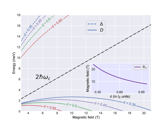
Figure 1: Solid lines: the calculated skyrmion-antiskyrmion excitation gap $D(B)$ [Eqs. 39 and 40; material parameters are $m_{e}^{*}=0.3m_{e}$ and $\kappa=8.5$] at different quantum well effective width $d$ parametrizing the 2D Fourier component ${\tilde{V}}(p)$ of the Coulomb vertex [see equation (2.29) and the specific expression for ${\tilde{V}}$ given in the text of section III]. Value $d$ is given in units of the magnetic length. Dash lines: the electron-exchange-hole gap $\Delta$ (see Ref. foot, ) calculated in the framework of the same approach/model. On the inset: the critical magnetic field $B_{cr}$, where $D$ vanishes [$D(B_{cr})=0$], is shown as function of parameter $d$.

We emphasize that the study presented is purely theoretical. However, it is worth noting that the actual situation is as follows: The conditions under which the $D$ value gives the main contribution to the creation energy of the skyrmion-antiskyrmion pair, and thereby to the transport gap, are hardly met in the QHSs currently investigated in experiments.ma14 ; va17 Indeed, in order to ignore the change of the Zeeman energy,

$$\delta E_{\rm Z}=\frac{\nu\,\epsilon_{\rm Z}}{2}\!\int\!\!d^{2}\!\mbox{{\boldmath$R$}}\,\left[1-n_{z}(\!\mbox{{\boldmath$R$}})\right],\vspace{-1.5mm}$$ (41)

and to neglect the Coulomb (Hartree) interaction between different charged domains ${G}$$\!{}_{\footnotesize{\mbox{\boldmath$R$}}_{i}}$ (determined only by the inter-domain repulsion at distances $|\mbox{\boldmath$R$}_{i}-\mbox{\boldmath$R$}_{j}|\gg l_{B}$),

$$V_{\rm H}=\displaystyle{\!\frac{\nu^{2}e^{2}}{2\kappa}\!\int\!\!\!\int\!\!\frac{d^{2}\!\!\mbox{{\boldmath$R$}}\,d^{2}\!\!\mbox{{\boldmath$R$}}^{\prime}}{|\!\mbox{{\boldmath$R$}}\!-\!\!\mbox{{\boldmath$R$}}^{\prime}|}\rho_{\mbox{\tiny T}}\!(\!\mbox{{\boldmath$R$}})\rho_{\mbox{\tiny T}}\!(\!\mbox{{\boldmath$R$}}^{\prime})}\vspace{-1.mm}$$ (42)

[see Eqs. 11 and 14, and also cf., e.g., Refs. so93, and by98, ], it is necessary that the ratio $\epsilon_{\rm Z}/(e^{2}/\kappa l_{B})$ be not simply small, but its smallness must be such that the logarithm $\ln{\!(e^{2}\!/\kappa l_{B}\epsilon_{\rm Z})}$ is large.by98 (See also Appendix A below.) An estimate, that is easy to make in the same way as it was done earlier in the works devoted to the $\nu\!=\!1$ ferromagnet,by98 leads to the conclusion: ‘classical’ corrections, given by Eqs. 41 and 42, become essentially smaller than the value 39–40 only in the situation where $\epsilon_{\rm Z}/(e^{2}\!/\kappa l_{B})\!<\!0.001$. (So then $\Lambda$ turns out to be well larger than $l_{B}$, indeed.) Whereas, even for GaAs/AlGaAs 2D structures the characteristic value is $\epsilon_{\rm Z}/(e^{2}\!/\kappa l_{B})\!\backsimeq\!0.01$, and for ZnO/MgZnO quantum wells we get it $\gtrsim\!0.03$.

Apparently, there are certain techniques that can reduce the value of $\epsilon_{\rm Z}$ experimentally; that is, to reduce effectively the Land$\acute{\mbox{e}}$ factor $g$ in actual experiments (see, for instance, Ref. ma96, ). Then the calculated value $D$ can correspond to the energy gap of creation of charge carriers, skyrmions and antiskyrmions, responsible for Ohmic transport in ZnO/MgZnO quantum heterostructures. More probable (even without artificial suppression of the Land$\acute{\mbox{e}}$ factor) is appearance of a spin-charge texture in the $\nu\!=\!2$ QH ferromagnet ground state near the critical field $B_{\rm cr}$, corresponding to the Stoner transition. This texture should be characterized by a local spin change with amplitude $\delta S\!>\!1$ and the correlation length $\Lambda\!>\!l_{B}$.

In conclusion, we note that only the 39–40 result, of microscopic calculation, where the exchange interaction is appropriately taken into account, can predict the Stoner transition to a paramagnet phase. Neither the Zeeman energy 41 nor the Hartree energy 42 (both smoothly growing with the magnetic field) give any grounds for the possibility of such a phase transformation.

The authors are grateful to A.V. Shchepetilnikov and A.B. Van’kov for useful discussion, and the Russian Science Foundation (Grant No. 22-12-00257) for support.

Appendix A The $O(3)$ nonlinear sigma model

For convenience, we review some relevant results of the classical field theory. In the framework of the nonlinear sigma (NL$\sigma$) model be75 ; ra89 , the density of ‘gradient’ energy $e(\mbox{{\boldmath$R$}})$ and topological density $\rho_{\mbox{\tiny T}}(\mbox{{\boldmath$R$}})$ are given by expressions

$$\begin{array}[]{l}\displaystyle{e(\mbox{{\boldmath$R$}})\!=\!\frac{J}{2}\left[\left(\partial_{X}\!{\vec{\,n}}\right)^{2}\!+\!\left(\partial_{Y}\!{\vec{\,n}}\right)^{2}\right]\vspace{.5mm}}\\ \qquad\qquad\qquad\displaystyle{\equiv\frac{J}{2}\!\!\left[\left(\!\!\mbox{ {\boldmath$\nabla$}}{\beta}\right)^{2}\!\!+\!\sin^{2}\!\!{\beta}\left(\!\mbox{{\boldmath$\nabla$}}{\alpha}\right)^{2}\right]}\,;\end{array}\vspace{-2.mm}$$ (43)

and

$${}\!\!\begin{array}[]{l}\displaystyle{\rho_{\mbox{\tiny T}}(\mbox{{\boldmath$R$}})=(4\pi)^{-1}{\vec{\,n}}\cdot\left(\partial_{X}\!{\vec{\,n}}\right)\times\left(\partial_{Y}\!{\vec{\,n}}\right)\vspace{.5mm}}\\ \displaystyle{\quad\equiv\,(4\pi)^{-1}\sin\!\beta\cdot\left(\partial_{X}\beta\cdot\partial_{Y}\alpha-\partial_{Y}\beta\cdot\partial_{X}\alpha\right)},\end{array}\vspace{-1.mm}$$ (44)

where ${\vec{n}}$ is the 3D unit vector 3, $\mbox{{\boldmath$\nabla$}}\equiv(\partial_{X},\partial_{Y})$, and $J$ is the spin stiffness – parameter undefined in the framework of the NL$\sigma$ model, which, however can be found microscopically (see Sec. III). Both values, $e(\mbox{{\boldmath$R$}})$ and $\rho_{\mbox{\tiny T}}(\mbox{{\boldmath$R$}})$, are also invariant with respect to substitution 4.

With the help of Eqs. 5 we find that $e(\mbox{{\boldmath$R$}})$ and $\rho_{\mbox{\tiny T}}(\mbox{{\boldmath$R$}})$ are expressed in terms of $(n_{X},n_{Y}\!,n_{Z})$ as well as in terms of $(n_{x},n_{y},n_{z})$ above, i.e. the equations of the NL$\sigma$ model are invariant with respect to rotation by a constant angle $\theta$. However, the limit values of $\vec{\,n}$ at $\mbox{{\boldmath$R$}}\!=\!0$ and $R\!=\!\infty$ are transformed into $n_{X}|_{R=0}\!=\!-\sin\theta,\>n_{Y}|_{R=0}\!=\!0,\>n_{Z}|_{R=0}\!=\!-\cos\theta$ and $n_{X}|_{R=\infty}\!=\!\sin\theta,\>n_{Y}|_{R=\infty}\!=\!0,\>n_{Z}|_{R=\infty}\!=\!\cos\theta$, respectively.

The main features of the NL$\sigma$ model are as follows:be75 (i) since the continuous, suitably behaved, function $\vec{\,n}(\mbox{{\boldmath$R$}})$ implements the mapping of the $\{{\hat{X}},{\hat{Y}}\}$ plane onto a unit sphere parametrized by angles $\alpha$ and $\beta$, the topological charge $q_{\mbox{\tiny T}}[\vec{\,n}]\!=\!\int\!\rho_{\mbox{\tiny T}}(\mbox{{\boldmath$R$}})d^{2}\!\mbox{{\boldmath$R$}}$ takes only integer-number values, either positive or negative, depending on the function $\beta(\mbox{{\boldmath$R$}})$, running through values from $\left.\beta(\mbox{{\boldmath$R$}})\right|_{R\!\to\infty}\!\!=\!0$ to $\beta(\mbox{{\boldmath$0$}})=m\pi$, where $m=\pm 1,\pm 2,...;\,$ (ii) the minima of the energy $E[\vec{\,n}]\!=\!\int\!e(\mbox{{\boldmath$R$}})d^{2}\!\mbox{{\boldmath$R$}}\,$, considered as a function of $\vec{\,n}(\mbox{{\boldmath$R$}})$, are determined by the $q_{\mbox{\tiny T}}$ values,

$$\mathop{\rm min}\nolimits{E[\vec{\,n}]}=4\pi J|q_{\mbox{\tiny T}}|\,.$$ (45)

It is known that $w=\!\cot{\!(\beta\!/\!2)}e^{i\alpha}$ represents an analytical functions of the variable ${\mathscr{Z}}=X+iY$.be75 This property and conditions of the physically appropriate behavior of the ${\vec{n}}(\alpha,\beta)$ vector considered as a function of $R$ enable to find an analytical form of $w({\mathscr{Z}})$. In particular, if ${\vec{n}}(\mbox{{\boldmath$R$}})$ has no singularities at finite $R$, then in the simplest but non-trivial case (i.e. when $w$ is not equal to a constant) the unit topological charge, $q_{\mbox{\tiny T}}\!=\!\pm\!1$, corresponds to a field where  be75

$$w={\mathscr{Z}}/\Lambda.\vspace{-1.mm}$$ (46)

Within the framework of the macroscopic approach used, the parameter $\Lambda$ controlling the size scale remains undetermined within the NL$\sigma$. model. From Eq. 46 it follows that in this case

$$\cos{\beta}=\frac{R^{2}-\Lambda^{2}}{R^{2}+\Lambda^{2}}\,,\quad\sin{\beta}=\pm\frac{2R\Lambda}{R^{2}+\Lambda^{2}}\,,\vspace{-3.mm}$$ (47)

$$\sin{\alpha}=\frac{Y}{R}\,,\quad\mbox{and}\quad\cos{\alpha}=\frac{X}{R}\,;$$ (48)

and the topological density 44 is

$$\rho_{\mbox{\tiny T}}=\pm\frac{\Lambda^{2}}{\pi(R^{2}+\Lambda^{2})^{2}}\,.\vspace{-2.mm}$$ (49)

Substituting expressions 47 and 49 into formulas 41 and 42 leads to the fact that integral 42 converges and is well defined for any finite value of $\Lambda$, whereas integral 41, at any nonzero $\epsilon_{\rm Z}$, diverges logarithmically for any finite $\Lambda$. The study by98 shows that actually the skyrmion should be characterized by two length scales: $\Lambda$ – the scale controlling the skyrmion ‘core’, and some value $l_{\rm sk}\sim(e^{2}/l_{B}\kappa\epsilon_{\rm Z})^{1/2}$ as a scale characterizing the decrease in density $\rho_{\mbox{\tiny T}}(R)$ on the ‘tail’ – at $R\gg\Lambda$. The divergent integral is cut off at length $l_{\rm sk}$ considered to be much larger than $\Lambda$, so that the subsequent minimization procedure by using $\Lambda$ as a variational parameter, gives the Zeeman 41 and Hartree 42 energies to logarithmic accuracy.by98

Appendix B Equivalences for the spatial derivatives of the spin-rotation matrix components

The spinor rotation matrix is  ll91

$${\hat{U}}(\mbox{\boldmath$R$})=\begin{pmatrix}\vspace{1.mm}\cos\!\frac{\beta}{2}\,e^{i(\alpha+\gamma)\!/2}&\sin\!\frac{\beta}{2}\,e^{-i(\alpha-\gamma)\!/2}\,\vspace{1.5mm}\\ -\sin\!\frac{\beta}{2}\,e^{i(\alpha-\gamma)\!/2}&\cos\!\frac{\beta}{2}\,e^{-i(\alpha+\gamma)\!/2}\,\end{pmatrix}.$$

The choice of functions $\alpha(\mbox{\boldmath$R$})$, $\beta(\mbox{\boldmath$R$})$ and $\gamma(\mbox{\boldmath$R$})$ is determined by our goal to find the lowest energy spin excitation. In particular, the dependence of angle $\gamma$ on coordinate $R$ cannot be ignored (i.e., for example, if considering it to be constant), even despite formal non-participation of $\gamma$ in determining the direction of the 3D unit vector [see. Eqs. 2 and 3].

Indeed, the additional ‘$\vec{\,\Omega}^{(l)}\!\!{\hat{\sigma}}_{l}$’ terms in Eq. 13, appearing due to the noncommutativity of the $\nabla$ and ${\hat{U}}\!(\mbox{\boldmath$R$})$ operators, are equal to $\displaystyle{-i{\hat{U}}^{\dagger}\mbox{\boldmath$\nabla$}{\hat{U}}\!\equiv\!\!\!\sum_{\,l=x,y,z}\!\!\!\mbox{\boldmath$\Gamma$}{}^{(l)}\!(\mbox{\boldmath$R$})\,\hat{\sigma}_{l}}$, where $\qquad\begin{array}[]{r}\;{}\;{}\qquad\displaystyle{\mbox{\boldmath$\Gamma$}{}^{(x)}\!=\left(-\sin{\alpha}\,\mbox{\small\boldmath$\nabla$}\beta+{\sin{\beta}\cos{\alpha}}\mbox{\small\boldmath$\nabla$}\gamma\right)\!/2},\vspace{1.mm}\\ {}\;{}\,\,\;\qquad\displaystyle{\!\mbox{\boldmath$\Gamma$}{}^{(y)}=\left(\cos{\alpha}\,\mbox{\small\boldmath$\nabla$}\beta+\sin{\beta}\sin{\alpha}\mbox{\small\boldmath$\nabla$}\gamma\right)\!/2},{}{}{}\end{array}$

and

$\begin{array}[]{r}\qquad\displaystyle{\!\mbox{\boldmath$\Gamma$}{}^{(z)}\!=(\vphantom{\mbox{\boldmath$\Gamma$}{}^{(z)}}\mbox{\small\boldmath$\nabla$}\alpha+\cos{\beta}\cdot\mbox{\small\boldmath$\nabla$}\gamma)\!/2\,}.\vspace{-0.mm}{}{}\end{array}$

If we suppose $\gamma\!=\,$const, then $\operatorname{rot}\!\mbox{\boldmath$\Gamma$}{}^{(z)}\!\equiv 0$ wherever $\alpha(\mbox{\boldmath$R$})$ is regular, which is considered to occur at any $\mbox{\boldmath$R$}\neq 0$). This leads only to a trivial case with zero topological density 44, i.e.to the ground state. At the same time, if assuming $\gamma=\alpha(\mbox{\boldmath$R$})$, we find out that: first, the non-physical singularity of $\mbox{\boldmath$\Gamma$}{}^{(z)}(\mbox{\boldmath$0$})$ (emerging due to uncertainty of the $\alpha$ value at the point $\mbox{\boldmath$R$}=0$, where $\cos{\beta(\mbox{\boldmath$0$})}=-1$) is canceled; second, the combination $\sum_{l}\!\left[\mbox{\boldmath$\Gamma$}{}^{(l)}\right]^{2}$ represents exactly the energy density defined in the framework of the $O(3)$ NL$\sigma$ model 43 (the latter is presumably suitable for a macroscopic description of extensive large-scale spin excitations); third, the functions $\alpha(\mbox{\boldmath$R$})$ and $\beta(\mbox{\boldmath$R$})$ may be chosen regular at any finite $R$, see below Eqs. 53. So replacing ${\vec{\Omega}}$${}_{\tiny{\mbox{\boldmath$R$}}}^{(l)}=\left.\mbox{\boldmath$\Gamma$}{}^{(l)}\right|_{\gamma=\alpha}$, we obtain

$${}\!{}\!{}\!\begin{array}[]{l}\displaystyle{\Omega_{\mbox{\tiny{\boldmath$R$}},\mu}^{(z)}}\!=\!\frac{1}{2}\left(\vphantom{{\Omega}_{\mu}^{(z)}}1+\cos{\!\mbox{$\beta$}}\right)\partial_{\mu}\mbox{$\alpha$}\,,\quad\mbox{and}\vspace{.5mm}\\ \displaystyle{\Omega_{\mbox{\tiny{\boldmath$R$}},\mu}^{(x)}}\!=\!-{\frac{1}{2}\sin{\mbox{$\alpha$}}{\vphantom{{\Omega}_{\mu}^{(z)}}}}\,\partial_{\mu}\mbox{$\beta$}+\!\displaystyle{\frac{\sin{\!\beta}}{2}{\vphantom{{\Omega}_{\mu}^{(z)}}}\!\cos{\mbox{$\alpha$}}\,\partial_{\mu}\mbox{$\alpha$}},\vspace{1.mm}\\ \displaystyle{\Omega_{\mbox{\tiny{\boldmath$R$}},\mu}^{(y)}}\!=\!{\frac{1}{2}\cos{\mbox{$\alpha$}}{\vphantom{{\Omega}_{\mu}^{(z)}}}}\,\partial_{\mu}\mbox{$\beta$}+\displaystyle{\frac{\sin{\!\beta}}{2}{\vphantom{{\Omega}_{\mu}^{(z)}}}\!\sin{\!\mbox{$\alpha$}}\,\partial_{\mu}\mbox{$\alpha$}},\vspace{-1.5mm}\end{array}$$ (50)

where $\mu=X$ or $Y$. The following identities take place for these values and their combinations determined by formulae 25:

$$\begin{array}[]{l}\operatorname{rot}{\vec{\Omega}}^{(z)}\!\equiv\!2\Omega_{X}^{(x)}\Omega_{Y}^{(y)}-2\Omega_{X}^{(y)}\Omega_{Y}^{(x)}\vspace{1.5mm}\\ \qquad\quad\,\,\equiv\displaystyle{\sin\!\beta\cdot\left(\partial_{X}\beta\cdot\partial_{Y}\alpha-\partial_{Y}\beta\cdot\partial_{X}\alpha\right)}\end{array}\vspace{-2.mm}$$ (51)

and

$$\Omega_{\pm}^{-}\Omega_{\mp}^{+}\equiv\frac{1}{2}\left[\sum_{\mu=X,Y\atop l=x,y}\!\!\!\left(\!{\Omega}^{(l)}_{\mu}\!\right)\!\!{\vphantom{\left({\vec{\Omega}}^{(l)}\pm\frac{1}{2}\!\operatorname{rot}{\vec{\Omega}}^{(z)}\right)}}^{2}\right]\pm\frac{1}{2}\operatorname{rot}{\vec{\Omega}}^{(z)}\vspace{-2.mm}$$ (52)

(the subscript …${}_{\mbox{\scriptsize\boldmath$R$}}$ is omitted). Using Eq. 43 we also find that

$$\sum_{\mu=X,Y\atop l=x,y}\!\!\!\left(\!{\Omega}^{(l)}_{\mu}\!\right)\!\!{\vphantom{\left({\vec{\Omega}}^{(l)}\pm\frac{1}{4}\!\operatorname{rot}{\vec{\Omega}}^{(z)}\right)}}^{2}\equiv\displaystyle{\frac{1}{4}\left[\left(\partial_{X}\!{\vec{\,n}}\right)^{2}\!+\!\left(\partial_{Y}\!{\vec{\,n}}\right)^{2}\right]},\vspace{-2.mm}$$ (53)

where $\vec{\,n}$ is the 3D unit vector presented by Eqs. 3 or 5.

References

• (1) S.L. Sondhi, A. Karlhede, S.A. Kivelson, and E.H. Rezayi, Phys. Rev. B 47, 16419 (1993).
• (2) S.E. Barret, G. Dabbagh, L.N. Pfeifer, K.W. West, and R. Tycko, Phys. Rev. Lett. 74, 5112 (1995); A. Schmeller, J.P. Eisenstein, L.N. Pfeiffer, and K.W. West, ibid  75, 4290 (1995); V. Bayot, E. Grivei, S. Melinte, M.B. Santos, and M. Shayegan, ibid  76, 4584 (1996).
• (3) See, e.g., J.J. Palacios, D. Yoshioka, and A.H. MacDonald, Phys. Rev. B 54, R2296 (1996).
• (4) D. Maryenko, J. Falson, Y. Kozuka, A. Tsukazaki, and M. Kawasaki, Phys. Rev. B 90, 245303 (2014); J. Falson, D.Maryenko, B. Friess, D. Zhang, and Y. Kozuka, Nat. Phys. 11, 347 (2015); A. B. Vankov, B. D. Kaysin, and I. V. Kukushkin, JETP Lett. 107, 106 (2018).
• (5) A.B. Vankov, B.D. Kaysin, and I.V. Kukushkin, Phys. Rev. B 96, 235401 (2017); ibid 98, 121412(R) (2018).
• (6) S. Dickmann and B.D. Kaysin Phys. Rev. B 101, 235317 (2020).
• (7) Yu.A. Bychkov, S.V. Iordanskii, and G.M. Eliashberg, JETP Lett. 33, 143 (1981); C. Kallin and B.I. Halperin, Phys. Rev. B 30, 5655 (1984).
• (8) See, e.g., W. Luo and R. Cote, Phys. Rev. B 88, 115417 (2013); W. Luo and T. Chakraborty, ibid 93, 161103(R) (2016).
• (9) R.B. Laughlin, Phys. Rev. Lett. 50, 1395 (1983); S.M. Girvin, A.H. MacDonald, and P.M. Platzman, Phys. Rev. B 33, 2481 (1986); J.K. Jain, Composite Fermions. Cambridge: Cambridge Univercity Press (2007).
• (10) E.M. Lifshitz and L.P. Pitaevskii, LANDAU AND LIFSHITZ: COURSE OF THEORETICAL PHYSICS, V 9; Statistical Physics, Theory of the Condensed State (Pt 2). (Butterworth-Heinemann, Oxford, 1991).
• (11) A.B. Migdal, Sov. Phys. JETP 5, 333 (1957).
• (12) I.V. Kukushkin, JETP 135, 448 (2022).
• (13) See Yu.A. Bychkov, A.V. Kolesnikov, T. Maniv, and I.D. Vagner, J. Phys.: Condens. Matter 10, 2029 (1998), and publications cited therein.
• (14) S.V. Iordanskii, S.G. Plyasunov, and V.I. Fal’ko, JETP 88, 392 (1999).
• (15) S. Dickmann. Phys. Rev. B 65, 195310 (2002).
• (16) A.H. MacDonald, H.C.A. Oji, and S.M. Girvin, Phys. Rev. Lett. 55, 2208 (1985); J.P. Longo and C. Kallin, Phys. Rev. B 47, 4429 (1993).
• (17) L.D. Landau and E.M. Lifschitz, Quantum Mechanics (Butterworth-Heinemann, Oxford, 1991).
• (18) This statement is true if function $F$ does not depend on the interaction of electrons belonging to different domains.
• (19) The calculation in Eq. 20 can be performed using, for instance, the excitonic representation for interaction operator 14.di20 After subsequent subtraction of the positive background energy, the result is
$$\!{}\!\begin{array}[]{l}E^{(0,\nu)}_{\rm int}\!(\!\mbox{\boldmath$R$})=\!{-\pi\!\sum_{\mbox{\scriptsize\boldmath$q$}}\!{\tilde{V}}(ql_{B})\left[\delta_{\nu,1}\vphantom{+\,l_{B}^{2}q^{2}\!/2}+\delta_{\nu,2}\left(\,2\right.\right.\vspace{0.mm}}\\ \quad\qquad\qquad\qquad\qquad\quad\left.\left.+\,l_{B}^{2}q^{2}\!/2\right)\right]e^{-q^{2}\l_{B}^{2}\!/2}.\end{array}\vspace{-3.mm}$$
${\tilde{V}}(p)$ is defined by equation 29 in the text. The summation is transformed by the integration: ${\small\sum}_{\mbox{\scriptsize\boldmath$q$}}...\!\to\!(N_{\phi}/2\pi)\!\int\!...\,l_{B}^{2}d^{2}\!\mbox{\boldmath$q$}\,$ [$N_{\phi}$ is given by Eq. 26]. In case parameter rsβˆΌβ„°C/Ο‰csimilar-tosubscriptπ‘Ÿπ‘ subscriptβ„°Csubscriptπœ”π‘r_{s}\!\sim\!{\mathscr{E}}_{\rm C}\!/\omega_{c}\, is considered to be small, then the result $E^{(0,\nu)}_{\rm int}$ above is asymptotically exact to the first order in rssubscriptπ‘Ÿπ‘ r_{s}.
• (20) W. Kohn, Phys. Rev. 123, 1242 (1961).
• (21) A. Pinczuk, B.S. Dennis, D. Heiman, C. Kallin, L. Brey, C. Tejedor, S. Schmitt-Rink, L.N. Pfeiffer, and K.W. West, Phys. Rev. Lett. 68, 3623 (1992).
• (22) This state is represented in the limit case of the lowest-energy spin-flip ($\delta S\!=\!-1$) magnetoexciton corresponding to the infinitely large 2D momentum. Its energy, under the $\epsilon_{\rm Z}\!=\!0$ condition, is given by equation: di20
$${}\!{}\Delta\!=\!{\int_{0}^{\infty}\!\tilde{V}(p)e^{-p^{2}\!/2}\left(1\!-\!\frac{p^{2}}{2}\!+\!\frac{p^{4}}{4}\right)p\,dp}\vspace{-2.mm}$$
(see the energy of the state designated as 𝒬1​1Β―β€‹βˆžβ€ β€‹|0⟩superscriptsubscript𝒬1Β―1†ket0{\cal Q}_{1\overline{1}{\bf\infty}}^{\dagger}|0\rangle in the publication cited).
• (23) D.K. Maude, M. Potemski, J.C. Portal, M. Heinini, L. Eaves, G. Hill, and M.A. Pate, Phys. Rev. Lett. 77, 4604 (1996).
• (24) A.A. Belavin and A. M. Polyakov, JETP Lett. 22, 245 (1975)].
• (25) For a review see R. Rajaraman, Solitons and Instantons (North-Holland, Amsterdam, 1989).