Neural Quantum Embedding:
Pushing the Limits of Quantum Supervised Learning

Abstract

Quantum embedding is indispensable for applying quantum machine learning techniques to classical data, and has substantial impacts on performance outcomes. In this study, we present Neural Quantum Embedding (NQE), a method that efficiently optimizes quantum embedding by leveraging classical deep learning techniques. NQE enhances the lower bound of the empirical risk, leading to substantial improvements in classification performance. Moreover, NQE improves robustness against noise. To validate the effectiveness of NQE, we conduct experiments on IBM quantum devices for image data classification, resulting in a remarkable accuracy enhancement from 0.52 to 0.96. Numerical analysis of the local effective dimension highlights that NQE improves the trainability and generalization performance of quantum neural networks. Furthermore, NQE achieves improved generalization in the quantum kernel method, as evidenced by a reduction in the upper bound of the expected risk.

I Introduction

Machine learning (ML) is ubiquitous in modern society, owing to its capability to identify patterns from data. For well-behaved data, simple learning algorithms such as linear regression and support vector machines are often sufficient to capture the underlying data distribution. In contrast, intricate and high-dimensional data require advanced learning algorithms, substantial computational power, and extensive training data. The overarching objective of machine learning is to construct models that can effectively learn the underlying distributions of complex real-world data. However, achieving this objective presents a substantial challenge.

Recent advances in quantum computing (QC) have led to the development of quantum machine learning (QML). QML aims to efficiently process complex data distributions by leveraging the computational benefits of quantum algorithms [1, 2, 3, 4, 5]. One potential benefit of QC relevant to ML is its ability to efficiently sample from certain probability distributions that are exponentially difficult for classical counterparts [6, 7, 8], as validated in several experiments [9, 10, 11]. Quantum sampling algorithms typically impose lower requirements on physical implementations, making them an attractive pathway for demonstrating the quantum advantage using Noisy Intermediate-Scale Quantum (NISQ) devices [12]. One of the primary rationales underpinning the potential of QML is as follows: if a quantum computer can efficiently sample from a computationally hard probability distribution, it is plausible that quantum computers can efficiently learn from data drawn from such distributions. This implies a potential quantum advantage, especially for data distributions that are computationally infeasible for classical models but easily tractable for quantum models.

While quantum data is naturally suited for QML tasks [5], most contemporary data science challenges involve classical data. Consequently, exploring the effectiveness of QML algorithms in learning from classical data constitutes a critical research focus. Notable examples of QML models tailored for classical data include Quantum Neural Network (QNN) and Quantum Kernel Method (QKM), both of which are specialized for supervised learning problems. QNN utilizes parameterized quantum circuit where the parameters are optimized through variational method [13, 14, 15, 16]. In contrast, QKM utilizes quantum kernel function to effectively capture the correlations within the data [17, 18].

In QML tasks involving classical data, an essential initial step is quantum embedding, which maps classical data into quantum states that a quantum computer can process. Quantum embedding is of paramount importance because it can significantly impact the performance of the learning model, including aspects such as expressibility [19], generalization capability [20], and trainability [21]. Therefore, selecting an appropriate quantum embedding circuit is crucial for the successful learning of the data with quantum models. To achieve a quantum advantage in machine learning, prevailing research emphasizes on designing quantum embedding circuits that are computationally challenging to simulate classically [17, 22]. In this work, we redirect attention to the data separability of embedded quantum states, utilizing trace distance, a tool in quantum information theory used to measure the distinguishability between quantum states [23, 24], as a figure of merit. Subsequent sections will show that the choice of a quantum embedding circuit inherently dictates a lower bound of empirical risk, independent of any succeeding trainable quantum circuits. Specifically, in the context of binary classification employing a linear loss function, the empirical risk is bounded from below by the trace distance between two ensembles of data-embedded quantum states representing different classes. Therefore, opting for a quantum embedding that maximizes trace distance—and thus, enhances distinguishability of states—facilitates improved training performance. Furthermore, a larger trace distance enhances resilience to noise, as the data-embedded quantum states reside farther from the decision boundary.

Conventional quantum embedding schemes are generally data-agnostic and do not guarantee high levels of data separability for a given dataset. To achieve a large trace distance, the use of trainable quantum embeddings is essential. Some efforts have explored trainable quantum embeddings by employing parameterized quantum circuits in both QNN [25] and QKM [26] frameworks. However, incorporating these quantum circuits increases the quantum circuit depth and the number of gates, making it less compatible with NISQ devices. Furthermore, the inclusion of trainable quantum gates during the quantum embedding phase increases the model’s susceptibility to barren plateaus [27], thereby adversely affecting the efficient training.

Given these considerations, we present Neural Quantum Embedding (NQE), an efficient method that leverages the power of classical neural networks to learn the optimal quantum embedding for a given problem. NQE can enhance the quantum data separability beyond the capabilities of quantum channels, thereby extending the fundamental limits of quantum supervised learning. Our approach avoids the critical issues present in existing methods, such as the increased number of gates and quantum circuit depth and the exposure to the risk of barren plateaus. Numerical simulations and experiment with IBM quantum devices confirm the effectiveness of NQE in enhancing QML performance in several key metrics in machine learning. These improvements extend to training accuracy, generalization capability, trainability, and robustness against noise, surpassing the capabilities of existing quantum embedding methods.

II Results

II.1 Lower Bound of Empirical Risk in Quantum Binary Classification

In supervised learning, the primary objective is to identify a prediction function $f$ that minimizes the true (expected) risk $R(f)=\mathbb{E}[l(f(X),Y)]$ with respect to some loss function $l$, where $X$ and $Y$ are drawn from an unknown distribution $D$. Given a collection of $N$ sample data $\{(x_{i},y_{i})\}$, the goal of learning algorithms is to find the optimal function $f^{*}$ that minimizes the empirical risk $R_{N}(f)=(1/N)\sum_{i=1}^{N}l(f(x_{i}),y_{i})$ among a fixed function class $F$, i.e., $f^{*}=\arg\min_{f\in F}R_{N}(f)$. Quantum supervised learning algorithms aim to efficiently find prediction functions with improved performance by exploiting the computational power of the quantum device.

A QNN is a widely used method for quantum supervised learning. In QNN, a classical input data $x$ is first embedded into a quantum state by applying a quantum embedding circuit to an initial ground state, resulting in $\ket{x}=\Phi(x)\ket{0}^{\otimes n}$. Next, a parameterized unitary operator, denoted as $U(\theta)$, is applied to transform the embedded quantum states, and the state is measured with an observable $O$. The measurement outcome serves as a prediction function for supervised learning algorithms, expressed as $f(x;\theta)=\bra{x}U^{\dagger}(\theta)OU(\theta)\ket{x}$ . Subsequently, using gradient descent or one of its variants, we search for the optimal parameter $\theta^{*}$ that minimizes the empirical risk. For a binary classification task with input data $x\in\mathbb{R}^{m}$ and its associated label $y\in\{-1,1\}$, we can predict the label of the new data $x_{\text{new}}$ using the rule $y_{\text{new}}=\text{sign}[f(x_{\text{new}};\theta^{*})]$.

Alternatively, we can consider this procedure as a quantum state discrimination problem involving two parameterized POVMs, denoted as $E_{\pm}(\theta)=(I\pm U^{\dagger}(\theta)OU(\theta))/2$. With these POVMs, the probabilities of obtaining measurement outcomes $\pm 1$ given an input data $x$ are computed as $P(E_{\pm}(\theta)|x)=\bra{x}E_{\pm}(\theta)\ket{x}$. Subsequently, the decision rule for the new data is determined as $y_{\text{new}}=\text{sign}[P(E_{+}(\theta)|x_{\text{new}})-P(E_{-}(\theta)|x_{\text{new}})]$. In such a scenario, a natural loss function is the probability of misclassification, which can be expressed as $l(f(x;\theta),y)=P(E_{\neg y}(\theta)|x)$. Considering a dataset of $N$ samples $S=\{x_{i}^{-},-1\}_{i=1}^{N^{-}}\cup\{x_{i}^{+},1\}_{i=1}^{N^{+}}$, the empirical risk becomes

$$L_{s} =\frac{1}{N}\bigg{[}\sum_{i=1}^{N^{-}}P(E_{+}(\theta)|x^{-}_{i})+\sum_{i=1}^{N^{+}}P(E_{-}(\theta)|x^{+}_{i})\bigg{]}$$

$$\geq\frac{1}{2}-D_{\text{tr}}(p^{-}\rho^{-},p^{+}\rho^{+}),$$ (1)

where $\rho^{\pm}=\sum\ket{x_{i}^{\pm}}\bra{x_{i}^{\pm}}/N^{\pm}$, $p^{\pm}=N^{\pm}/N$, and $D_{\text{tr}}(\cdot\;,\cdot)$ denotes the trace distance [28]. It is important to note the contractive property of the trace distance given by

$$D_{\text{tr}}(\Lambda(\rho_{0}),\Lambda(\rho_{1}))\leq D_{\text{tr}}(\rho_{0},\rho_{1}),$$ (2)

for any positive and trace-preserving (PTP) map $\Lambda$ [29]. Based on the above, we now emphasize two crucial points.

1. The empirical risk is lower bounded by the trace distance between two data ensembles $p^{-}\rho^{-}$ and $p^{+}\rho^{+}$. This bound is completely determined by the initial quantum embedding circuit, regardless of the structure of the parameterized unitary gates $U(\theta)$ applied afterwards.

2. The minimum loss is achieved when $\{E_{-}(\theta),E_{+}(\theta)\}$ is a Helstrom measurement. Therefore, the training of a quantum neural network can be viewed as a process of finding the Helstrom measurement that optimally discriminates between the two data ensembles.

Designing a quantum embedding that maximizes the trace distance is of paramount importance since it minimizes the lower bound of the empirical risk. This becomes especially important in NISQ applications, as non-unitary quantum operations, such as noise, strictly reduce the trace distance between two quantum states [23, 24]. Therefore, there is a clear need for a trainable, data-dependent embedding that can maximize the trace distance.

Several works have proposed combining a set of parameterized quantum gates and a conventional quantum embedding circuit as a means to create a trainable unitary embedding [25, 30, 31]. However, the use of parameterized quantum gates comes with several drawbacks. Firstly, it results in an increase in the number of gates and the depth of the quantum circuit. This not only increases computational costs but also makes the quantum embedding more susceptible to noise. Furthermore, the method is prone to encountering barren plateaus, which pose a fundamental obstacle to scalability [27, 21]. Secondly, the trainable unitary embedding is highly restricted in enhancing the maximum trace distance of embedded quantum states (see Supplementary Information). It is crucial to note that none of the existing quantum embeddings can guarantee the effective separation of two data ensembles in the Hilbert space with a large distance.

II.2 Neural Quantum Embedding

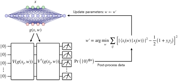
Figure 1: Overview of the NQE training. The unitary transformation that maps $x_{i}$ to the quantum feature space is determined by the output of a classical neural network denoted by $g(x_{i},w)$, where $w$ represents trainable parameters. The resulting quantum state is $|x_{i}(w)\rangle=V(g(x_{i},w))|0\rangle^{\otimes n}$. The goal of the training is to produce mapping functions that can separate the two classes of data into two orthogonal subspaces. Efficient calculation of the fidelity between the two quantum states produced by the feature map is performed using a quantum computer.

Neural Quantum Embedding utilizes a classical neural network to maximize the trace distance between two ensembles $D_{\text{tr}}(p^{-}\rho^{-},p^{+}\rho^{+})$. It can be expressed as $\Phi_{\mathrm{NQE}}:x\rightarrow\ket{x}=V(g(x,w))\ket{0}^{\otimes n}$,

where $V$ is a general quantum embedding circuit and $g:\mathbb{R}^{m}\times\mathbb{R}^{r}\rightarrow\mathbb{R}^{m^{\prime}}$ is a classical neural network that transforms the input data $x$ using $r$ trainable parameters.

By choosing $m^{\prime}<m$, we can bypass additional classical feature reduction methods, such as principal component analysis (PCA) or autoencoders, typically employed prior to quantum embedding due to the current limitations on the number of reliably controllable qubits in quantum devices. Ideally, the loss function should directly contain the trace distance. However, calculating it is computationally expensive even with the quantum computer. Therefore, we used an implicit loss function derived from a fidelity measure, which is expressed as

$$l_{\text{fid}}((x_{i},y_{i}),(x_{j},y_{j}))=\left[\left|\innerproduct{x_{i}}{x_{j}}\right|^{2}-\frac{1}{2}\left(1+y_{i}y_{j}\right)\right]^{2}.$$ (3)

This fidelity loss can be efficiently computed using the swap test [32] or directly measuring the state overlap (see Figure 1).

While NQE is not restricted by the choice of the quantum embedding circuit, we specifically focus on improving the ZZ feature embedding [17], which is constructed by repeating an Instantaneous quantum polynomial (IQP) circuit [33] $L>1$ times. The unitary operator corresponding to this embedding is expressed as

$$V(\phi(x))=\bigg{[}\exp\bigg{(}i\sum_{i}\phi_{i}(x)Z_{i}+i\sum_{i,j}\phi_{i,j}(x)Z_{i}Z_{j}\bigg{)}H^{\otimes n}\bigg{]}^{L}.$$ (4)

The use of this embedding is prevalent due to the conjectured intractability of its classical simulation. It has been extensively explored in the field of quantum machine learning, including theoretical investigations [15, 34, 35] as well as practical applications in areas like drug discovery [36, 37], high energy physics [38, 39], and finance [40, 41]. The most commonly used functions for $\phi$ are $\phi_{i}(x)=x_{i}$ and $\phi_{i,j}(x)=(\pi-x_{i})(\pi-x_{j})/2$ [17, 15], but these choices are made without justifications. Although Ref. [42] numerically illustrates that the choice of $\phi$ can significantly impact the performance of QML algorithms, it does not provide guidelines for selecting an appropriate $\phi$ for the problem at hand. NQE effectively solves this limitation by replacing mapping functions with a trainable classical neural network.

While optimizing the ZZ feature embedding through NQE requires the use of a quantum computer due to the computational hardness of the loss function, there are certain embeddings that can be optimized solely on a classical computer. An instance of this is the amplitude encoding [43, 44, 45, 46, 47], where the corresponding loss function for NQE can be computed by taking the dot product of two vectors.

II.3 Experimental Results

Figure 2: (a) Schematic representation of the quantum circuit used in the experiments. The green section indicates the Neural Quantum Embedding (NQE), which transforms classical data $x_{i}$ into quantum state $|x_{i}\rangle$. The blue section represents the Quantum Convolutional Neural Network (QCNN) architecture. (b) Plot depicting the evolution of the trace distance between two ensembles of quantum states embedded by the NQE models during training on the ibmq_toronto device, compared to the trace distance from conventional quantum embedding without NQE. (c) Noiseless QCNN simulation results. (d) The results from QCNN experiments conducted on IBM quantum devices. In (c) and (d), the blue solid, red dashed green dash-dotted lines represent the mean training loss histories for conventional ZZ feature embedding, PCA-NQE, and NQE, respectively. The shaded regions in the figure represent one standard deviation from the mean. These values are acquired from five repetitions of each QCNN training with random initialization of parameters. The thicker versions of these lines indicate the theoretical lower bounds for each method.

This section presents experimental results that demonstrate the effectiveness of NQE in enhancing QML algorithms. To this end, we employed a four-qubit Quantum Convolutional Neural Network (QCNN) for the task of classifying the digits 0 and 1 within the MNIST dataset [48], a well-established repository of handwritten digits. We conducted experiments using both noiseless simulations and quantum devices accessible through the IBM cloud service. The experiment unfolds in three main phases: the application of NQE, the training of the QCNN with and without NQE models, and the assessment of classification accuracies for the trained QCNN with and without NQE models.

We compared NQE against the conventional ZZ feature embedding with the aforementioned function $\phi_{i}(x)=x_{i}$ and $\phi_{i,j}(x)=(\pi-x_{i})(\pi-x_{j})/2$. Due to the limited number of qubits that can be manipulated reliably in current quantum devices, it is often necessary to reduce the number of features in the original data before embedding it as a quantum state. To address this issue, we tested two different NQE structures for incorporating dimensionality reduction. In the first approach, which we refer to as PCA-NQE, we applied PCA to reduce the number of features before passing them to the neural network. In the second approach, which we simply refer to as NQE, dimensionality reduction was directly handled within the neural network by adjusting the number of input and output nodes accordingly. For both PCA-NQE and NQE, classical neural networks produce eight dimensional vectors, which are then used as rotational angles for the four-qubit ZZ feature embedding. These two methods differ in their input requirements: PCA-NQE takes four-dimensional vectors as input, requiring classical feature reduction, while NQE accepts the original 28-by-28 image data, bypassing the need for additional classical preprocessing. Further details on the structure of the ZZ feature embedding circuit and the classical neural networks used for NQE methods are provided in the Methods section.

The goal of NQE training is to maximize the trace distance between the two sets of data ensembles, thereby minimizing the lower bound of the empirical risk. Figure 2(b) displays the trace distance as a function of NQE training iterations, acquired from ibmq_toronto. It is evident that both PCA-NQE and NQE effectively separate the embedded data ensembles and enhance the distinguishability of quantum state representing different classes, even in the presence of noise in the real quantum hardware. After optimization, PCA-NQE and NQE yield trace distances of 0.840 and 0.792, respectively, which are significantly improved compared to the conventional ZZ feature embedding with a distance of 0.273. Consequently, the lower bound of the empirical risk is significantly reduced to 0.08 and 0.104, respectively, from the original value of 0.364.

The training of the QCNN circuit provides additional evidence supporting the effectiveness of NQE in QML. Figure 2(c) presents the results of noiseless QCNN simulations. In this figure, the blue solid, red dashed, green dash-dotted lines represent the mean training loss histories for conventional ZZ feature embedding, PCA-NQE, and NQE, respectively. The thicker versions of these lines indicate the theoretical lower bounds for each method. The mean values are calculated from five repetitions of each QCNN training with random initialization of parameters. The shaded regions in the figure illustrate one standard deviation from the mean. The empirical risks for all models converge toward their respective theoretical minima, affirming that the trained QCNN adequately approximates optimal Helstrom measurements. Classification accuracies achieved on the test dataset are shown in the table within the figure. NQE methods led to significant enhancements, as demonstrated by reduced empirical risks and improved classification accuracies. Note that in some instances, the training loss falls below the theoretical lower bound of empirical risk. This occurs because the training loss is computed from a randomly sampled mini-batch of data in each iteration.

Figure 2(d) presents the mean QCNN training loss histories obtained using IBM quantum devices. The mean values are calculated from three independent trials on ibmq_jakarta, ibmq_perth, and ibmq_toronto devices with random initialization of parameters. The shaded regions in the figure illustrate one standard deviation from the mean. The presence of noise and imperfections in the quantum devices prevents the empirical risks from reaching their theoretical lower bounds. Nonetheless, the training performance is significantly improved by NQE. Notably, for both NQE methods, the empirical risk rapidly approaches or even falls below the theoretical limit of the conventional method. This result underscores that, even on the current noisy quantum devices, our method can outperform the theoretical optimum of the ZZ feature map without any additional quantum error mitigation. Moreover, a substantial improvement in classification accuracy was recorded, reaching 96% (PCA-NQE) and 90% (NQE), whereas the conventional method achieved only 52%. These findings demonstrate that NQE enhances the noise resilience of QML models, improving the utility of NISQ devices. Comprehensive details of these experiments are provided in Methods.

II.4 Effective Dimension

As demonstrated thus far, NQE has proven to be an efficient method for reducing the lower bound of empirical risk. While this advancement enhances the ability to learn from data, another essential measure of successful machine learning is the generalization performance, that is, the ability to make accurate predictions on unseen data based on what has been learned. The simulation and experimental results presented in the previous section already indicate an improvement in prediction accuracy on test data with the implementation of NQE. In this section, we provide additional evidence of improved generalization performance by analyzing the effective dimension (ED) [49, 15, 50] of a QML model constructed with and without NQE. Intuitively, ED quantifies the number of parameters that active in the sense that they influence the outcome of its statistical model.

To investigate this further, we focus on the local effective dimension (LED) introduced in Ref. [50], as it takes into account the data and learning algorithm dependencies and is computationally more convenient. Importantly, the LED exhibits a positive correlation with the generalization error, allowing for straightforward interpretation of the results: a smaller LED corresponds to a smaller generalization error, and vice versa. Our numerical investigation employs a four-qubit QNN (see Methods), and the results are presented in Fig. 3. In the figure, the green solid and purple dashed lines represent the mean local effective dimension of the tested QML model with and without NQE, respectively. The mean values are computed from 200 trials, where each trial consists of ten artificial datasets, and for each dataset, the experiment is repeated 20 times with random initialization of parameters. The shaded areas in the figure represent one standard deviation. The simulation results unequivocally demonstrate that NQE consistently reduces the LED in all 200 instances tested and across a wide range of training data sizes, signifying an improvement in generalization performance.

Figure 3: The local effective dimension for the circuit with (solid green) and without (dashed blue) NQE. These results are based on ten sets of experiments, each on a distinct artificial dataset with 20 repetitions with random initialization of parameters. The reported values represent the average across all 200 experiments.

The effective dimension can also be interpreted as a measure of the volume of the solution space that a specific model class can encompass. A smaller effective dimension in a QML model implies a reduced volume of the solution space. This observation is particularly relevant as it suggests that models with smaller effective dimensions are less prone to encountering barren plateaus [51]. Consequently, the simulation results further indicate that NQE not only enhances generalization performance but also improves the trainability of the model. Further evidence substantiating this improvement for both QNN and QKM will be presented in a later section.

II.5 Generalization in Quantum Kernel Method

Up to this point, the investigation of NQE has primarily focused on its application within the context of quantum neural networks. In this section, we extend the analysis to demonstrate that NQE also enhances the performance of the quantum kernel method. Given a quantum embedding, the kernel function can be defined as

$$k^{Q}(x_{i},x_{j})=\left|\innerproduct{x_{i}}{x_{j}}\right|^{2},$$ (5)

which can be computed efficiently on a quantum computer. The quantum kernel method refers to an approach that uses the kernel matrix $K^{Q}$, of which each entry is the kernel of the corresponding data points, in a method like a classical support vector machine [17, 34]. The potential quantum advantage of such approach is based on the hardness to compute certain quantum kernel functions classically [17, 33, 18].

The quantum kernel method attempts to determine the function $f(x;W)=\text{Tr}(W|x\rangle\langle x|)$ to predict the true underlying function $h(x)$ for unseen data $x$. The optimal parameters $W^{*}$ are obtained by minimizing the cost function

$$W^{*}=\operatorname*{arg\,min}_{W\in\mathbb{C}^{2^{n}\times 2^{n}}}\left(f(x;W)-h(x)\right)^{2}-\lambda||W||_{\text{F}}^{2},$$ (6)

where $||\cdot||_{\text{F}}$ is the Frobenius norm. The second term is the regularization term with a hyperparameter $\lambda$. The purpose of including the regularization term is to reduce the generalization error at the expense of the training error. Specifically, considering the true error $R(W)=\mathbb{E}_{x}|f(x;W)-h(x)|$, and the training error $R_{N}(W)=\sum_{i=1}^{N}|f(x_{i};W)-h(x_{i})|/N$, the generalization error is upper-bounded as

$$\left|R(W)-R_{N}(W)\right|\leq\mathcal{O}\left(\frac{||W||_{\text{F}}}{\sqrt{N}}\right).$$ (7)

The optimal $W^{*}$ can be expressed as $W^{*}=\sum_{i=1}^{N}\sum_{j=1}^{N}h(x_{i})(K^{Q}+\lambda I)^{-1}_{i,j}|x_{j}\rangle\langle x_{j}|$. Here, the employment of NQE affects $W^{*}$ as both $K^{Q}$ and $|x_{j}\rangle$ vary with the quantum embedding. We performed empirical evaluations to assess the effectiveness of NQE in reducing $G=||W||_{\text{F}}/\sqrt{N}$ and thereby improving the upper bound of the generalization error. For these evaluations, we utilized both PCA-NQE and NQE optimized on ibmq_toronto quantum hardware, as discussed earlier. Subsequently, we computed the quantum kernel matrices $K^{Q}$ with and without NQE models through numerical simulations. Figure 4 shows the generalization error bound $G$ obtained under the ZZ feature embedding with and without NQE across various regularization parameters $\lambda$. The results clearly demonstrate that NQE effectively reduces the upper bound of the generalization error in quantum kernel methods.

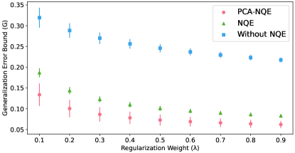
Figure 4: A comparative analysis of the generalization error bound $G$ with varying regularization weights $\lambda$. This plot illustrates the performance enhancement – lower generalization error bound – when employing NQE (green triangles) and PCA-NQE (red circles) over conventional methods without NQE (blue squares) in quantum kernel methods. PCA-NQE and NQE were optimized on the ibmq_toronto quantum hardware. The error bound G was determined based on five independent numerical simulations, presenting both the mean and one standard deviation of G.

II.6 Expressibility and Trainability

In both QNN and QKM, there exists a trade-off between expressibility and trainability. In the QNN framework, highly expressive quantum circuits often leads to barren plateaus, characterized by exponentially vanishing gradients, which severely hinders the trainability of the model [27, 51]. In the QKM framework, highly expressive embedding induces a quantum kernel matrix whose elements exhibit an exponential concentration [21]. Specifically, the concentration of quantum kernel element $K^{Q}_{i,j}=k^{Q}(x_{i},x_{j})$ can be expressed by Chebyshev’s inequality,

$$\mathrm{Pr}\left[\left|K^{Q}_{i,j}-\mathbb{E}\left[K^{Q}_{i,j}\right]\right|\geq\delta\right]\leq\frac{\mathrm{Var}\left[K^{Q}_{i,j}\right]}{\delta^{2}}$$ (8)

for any $\delta>0$. The quantum kernel element $K^{Q}_{i,j}$ arising from highly expressive quantum embedding displays an exponentially reduction in variance as the number of qubits increases. Consequently, an exponentially large number of quantum circuit executions is necessary to accurately approximate the quantum kernel matrix $K^{Q}$. This poses a significant challenge in the efficient implementation of QKM.

NQE addresses this challenge by constraining quantum embedding to ensure large distinguishability. NQE strategically limits the expressibility of the embedded quantum states, thereby enhancing the trainability of QML models. This improvement is achieved by exploiting the prior knowledge that a quantum embedding with large distinguishability can effectively approximate the true underlying function.

Figure 5(a) shows comparisons of the expressibility of embedded quantum states induced from PCA-NQE, NQE, and quantum embedding without NQE. Figure 5(b) shows comparisons of the variance of quantum kernel elements, arising from PCA-NQE, NQE, and quantum embedding without NQE. Here, PCA-NQE and NQE are optimized with ibmq_toronto as described in the earlier subsection. We observe a notable decrease in the expressibility and an increase in the variance of quantum kernel elements when NQE models are employed. These results underscores the effectiveness of NQE in enhancing the trainability of QML models within both QNN and QKM frameworks.

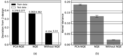
Figure 5: (a) A comparative analysis of expressibility with and without NQE models. The deviation from unitary 2-design is depicted, where a smaller deviation indicates higher expressibility. The deviation is derived from 12,665 (2,115) MNIST training (test) data results. (b) A comparative analysis of the variance of quantum kernel elements with and without NQE models. The variance was computed from the off-diagonal elements of the quantum kernel matrix $K^{Q}$, constructed from 1,000 samples of MNIST datasets. The mean and one standard deviation from five independent iterations are shown. For both (a) and (b), NQE models are optimized using the ibmq_toronto quantum device.

III Discussion

In this study, we investigated the crucial role of quantum embedding, an essential step in applying quantum machine learning to classical data. In particular, we highlighted how quantum data separability, namely the distinguishability of quantum states representing different classes, determines the lower bound of training error and affects the noise resilience of quantum supervised learning algorithms. Motivated by these results, we introduced Neural Quantum Embedding (NQE), which utilizes the power of classical neural network and deep learning to enhance data separability in the quantum feature space, thereby pushing the limits of quantum supervised learning. NQE is versatile in the sense that it can be integrated into all existing quantum data embedding methods, such as amplitude encoding, angle encoding, and Hamiltonian encoding. The training performance achieved by NQE is guaranteed to be at least as good as those that do not use it and rely on a fixed embedding function. This is because if the fixed embedding function happens to be the optimal one for the given data, NQE will learn to use it. Experimental results on IBM quantum hardware demonstrate that NQE significantly enhances quantum data separability, as quantified by increased trace distance between two ensembles of quantum states. Utilizing NQE led to a significant reduction in training loss and an improvement in accuracy and noise resilience in the MNIST data classification tasks. Notably, the experimental results achieved by NQE-enabled QML models outperformed the theoretical optimal of the conventional ZZ feature embedding that does not employ NQE.

A significant portion of current research in QML focuses on the trade-off between the expressibility and trainability of variational circuits within quantum neural networks. For a QML model to be effective, it must possess a high degree of expressibility, which ensures that it can approximate the desired solution with considerable accuracy. Concurrently, the model should be trainable, enabling optimization via a gradient descent algorithm or its variants. However, expressibility and trainability present a trade-off: high expressibility typically leads to reduced trainability  [51, 21, 27]. This trade-off constitutes a significant challenge in advancing QML. To address this challenge, a strategic approach is to utilize problem-specific prior knowledge. For example, Refs. [52, 53] deliberately construct variational circuits with limited expressibility, yet ensures the inclusion of the desired solution, by harnessing data symmetry. However, such method is not universally applicable to general datasets that do not presents any symmetry or group structure. NQE offers an effective solution to this challenge by optimizing the quantum data embedding process. As elucidated in the Results section, a good approximation of the true underlying function can only be achieved with quantum embeddings that ensure high distinguishability of the data. By using this prior knowledge, NQE constrain the quantum embedding to those that allows large distinguishability between quantum states that present the data. Consequently, the embedded quantum states from NQE are less expressive, resulting in an improvement in trainability.

The ultimate goal of machine learning is to construct a model that not only classifies the training data accurately (optimization) but also generalizes well to unseen data. In conventional machine learning, a trade-off typically exists between optimization and generalization [54]. However, our experimental results indicate that the incorporation of NQE markedly enhances both optimization and generalization metrics. This improvement is evidenced by reduced training error, reduced test error, diminished local effective dimension, and a reduced rank of the kernel matrix. Consequently, NQE presents a robust methodology for optimizing learning performance while preserving strong generalization capabilities.

Further research is necessary to explore the impact of the type or architecture of neural networks on the performance of NQE, and its optimization for specific types of target data. For instance, investigating the applicability of Recurrent Neural Networks (RNNs) for handling sequential data and Convolutional Neural Networks (CNNs) for image data remains an interesting avenue for future work. The incorporation of structure learning introduced in Ref. [55] with NQE is noteworthy as it can further improve the embedding. However, one must consider the trade-off between performance and the computational overhead introduced by the structure learning. As an alternative to NQE, enhancing quantum data separability can be achieved by implementing a probabilistic non-TP embedding [56]. Comparing this approach with NQE or exploring their combination for potential enhancements represents a valuable direction for future investigation.

Methods

NQE structures and training

The PCA-NQE method employs Principal Component Analysis (PCA) to extract four features from the original data. It then passes these features to a fully connected neural network with two hidden layers, each containing 16 nodes. The neural network has eight output nodes, corresponding to eight numerical values used as quantum gate parameters for the embedding. The rectified linear unit (ReLU) function serves as the non-linear activation. In contrast, NQE (without PCA) utilizes a 2-dimensional convolutional neural networks (CNN) which takes original data as an input. After each convolutional layer, we used 2D max pooling to reduce the dimension of the data. The dimension of the nodes in each layer are 28 by 28, 14 by 14, 7 by 7, and 8, respectively.

The classical neural networks of the NQE models are optimized by minimizing the implicit loss function $l_{\mathrm{fid}}((x_{i},y_{i}),(x_{j},y_{j}))$ given in Eq. (3), where $i$ and $j$ are the indices of the randomly selected training data. For the four-qubit real device experiments, the NQE models were trained for 50 iterations using the stochastic gradient descent with a learning rate of 0.1 and a batch size of 10. The loss function was evaluated on ibmq_toronto with the selection of four qubits based on the highest CNOT fidelities. For the ZZ feature embedding circuits, we configured the total number of layer ($L$) to 1 and applied two qubit gates only on the nearest neighboring qubits to avoid an excessive number of CNOT gates.

Classification with QCNN

In the noiseless simulation setting, we utilized QCNN circuits featuring a general SU(4) convolutional ansatz (refer to Fig. 2 (i) in Ref. [57]). The optimization of circuit parameters was performed over 1,000 iterations using the Nesterov momentum algorithm with a learning rate of 0.01 and a batch size of 128. Each simulation was repeated five times with random parameter initialization.

For experiments on IBM quantum hardware, QCNN circuits were configured with a basic convolutional ansatz comprising two $R_{y}(\theta)$ gates, where $R_{i}(\theta)$ represent a single-qubit rotation around the $i$-axis of the Bloch sphere by an angle $\theta$, and a CNOT gate (refer to Fig. 2 (a) in Ref. [57]). To minimize circuit depth, pooling gates were omitted. Moreover, the QCNN architecture was designed to allow only nearest-neighbor qubit interactions, eliminating the need for qubit swapping.

The training on quantum hardware consisted of 50 optimization iterations, using Nesterov momentum gradient descent with a learning rate of 0.1 and a batch size of 10. Experiments were conducted on three distinct quantum devices: ibmq_jakarta, ibmq_toronto, and ibmq_perth.

Performance evaluation was carried out by assessing the classification accuracy of the trained QCNN models on a separate test set comprising 500 data points. This assessment was executed across three different quantum devices: ibmq_lagos, ibmq_kolkata, and ibmq_jakarta.

Effective Dimension

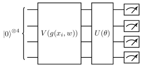
Figure 6: Quantum circuit used for evaluating the local effective dimension. The feature map, denoted by $V(g(x_{i},w))$, acts on the initial state $\ket{0}^{\otimes 4}$ to encode the input vector $x_{i}$. Subsequently, a parameterized unitary transformation $U(\theta)$ is applied to evolve the state, with the parameters $\theta$ chosen to minimize a specific loss function.

The analysis of the effective dimension utilizes the QNN architecture depicted in Fig. 6. The ZZ feature map, as explained in Eq. 4 and depicted in Fig. 7, is used for mapping classical data to quantum states. When NQE is not used, $g_{j}=x_{ij}$, which is the $j$th component of the input vector $x_{i}$, and the quantum embedding becomes equivalent to Eq. (4) with $L=1$. When NQE is turned on, $g_{j}=g_{j}(x_{i},w)$, which is the $j$th component of the output vector generated by a three-layer neural network. This output vector can be expressed as $g(x_{i},w)=\sigma(w^{(1)}{\sigma(w^{(0)}x_{i}+b^{(0)})}+b^{(1)})$. In this equation, $w^{(0)}\in\mathbb{R}^{12\times 4}$, $w^{(1)}\in\mathbb{R}^{4\times 12}$, $b^{(0)}\in\mathbb{R}^{12}$ and $b^{(1)}\in\mathbb{R}^{4}$ are the trainable parameters of the network, and $\sigma$ stands for the ReLU activation function.

The parameterized unitary operator of the QNN used in this analysis, represented as $U(\theta)$ Fig. 6, is shown in Fig. 8. This circuit design is attractive for several reasons. First, it offers a high degree of expressibility and entangling capability while maintaining a relatively small number of gates and parameters [58]. In addition, this design is hardware-efficient [59, 16], as it relies solely on single-qubit rotations and CNOT operations between adjacent qubits.

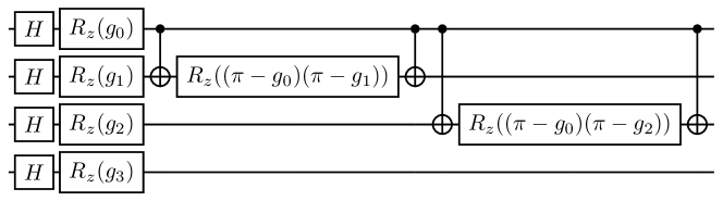
(a)

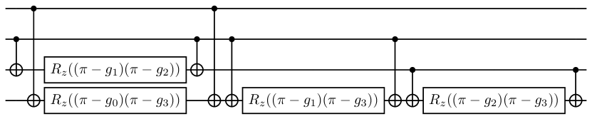
(b)

Figure 7: Quantum circuit diagram for the trainable ZZ feature map $V(g(x_{i},w))$. It uses mapping functions $g_{j}\in g(x_{i},w)$ to encode the input vector $x_{i}$.

The analysis encompassed ten artificial binary datasets, each containing 400 samples. These datasets, characterized by four features and four clusters per class, were generated through the make_classification function from the Scikit-Learn library [60]. The NQE model was trained for 100 iterations using the Adam optimizer [61] with a batch size of 25.

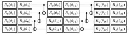
Figure 8: Parameterized quantum circuit layout for the QNN, which is represented as $U(\theta)$ in Fig. 6.

The local effective dimension [50] was determined using the get_effective_dimension function from the LocalEffectiveDimension class in Qiskit [62].

Generalization in Quantum Kernel Method

The analysis of generalization error in quantum kernel method was conducted in three steps: loading of the dataset, computation of the quantum kernel matrix with and without NQE, and calculation of generalization error bound with and without NQE. The experiments tested both PCA-NQE and NQE, and the neural network parameters were optimized on the ibmq_toronto processor, as detailed in the previous sections.

During the dataset loading phase, binary datasets containing $N=1,000$ samples from classes {0,1} were constructed from the MNIST dataset. For both PCA-NQE and the conventional quantum embedding without NQE, dimensionality reduction was performed on each dataset, reducing it to four features using PCA. In contrast, the NQE utilized the original 28x28 image datasets.

Next, the quantum kernel matrix $K^{Q}$ was constructed, where each element captured the fidelity overlap between pairs of data-embedded quantum states. This fidelity overlap was computed using Pennylane [63] numerical simulation. Since different quantum embedding techniques yield different state overlaps, we obtained three distinct quantum kernel matrices: one without NQE, one with PCA-NQE, and one with NQE.

Finally, for each of the quantum kernel matrices, the corresponding upper bound of the generalization error $G=\sqrt{||W^{*}||^{2}_{\text{F}}/N}$ was calculated. Here, $||W^{*}||^{2}_{\text{F}}$ can be expressed as $||W^{*}||^{2}_{\text{F}}=\sum_{i}\sum_{j}\left[(K^{Q}+\lambda I)^{-1}K^{Q}(K^{Q}+\lambda I)^{-1}\right]_{i,j}y_{i}y_{j}$, where $y_{i}$ represents the label associated with the data $x_{i}$.

The experimental procedure was repeated five times with different 1,000 samples of data. The mean and one standard deviation of the outcome generalization error bound is plotted in Figure 4.

Expressibility and Trainability

The expressibility were quantified as the Hilbert-Schmidt norm of the deviation from unitary 2-design [58, 51]. More specifically, the deviation is given as,

$$A=\int_{\textbf{Haar}}(|\psi\rangle\langle\psi|)^{\otimes 2}d\psi-\int_{\mathcal{E}}(|\phi\rangle\langle\phi|)^{\otimes 2}d\phi,$$ (9)

where the first integral is taken over the Haar measure, and the second integral is taken over ensemble of data embedded quantum states, $\mathcal{E}$. We then define the deviation norm, $\epsilon=\sqrt{\text{Tr}(A^{\dagger}A)}$, where a small $\epsilon$ indicates a highly expressive quantum embedding and vice versa. During the experiment, NQE and PCA-NQE are optimized utilizing the ibmq_toronto hardware. The value of $\epsilon$ was numerically computed for ensembles of training and test datasets of classes {0,1} from MNIST data, utilizing 12,665 instances for training data and 2,115 for test data. The results are shown in Figure 5(a).

To determine the variance of the quantum kernel elements, we initially computed quantum kernel matrix $K^{Q}$ using PCA-NQE, NQE, and quantum embedding without NQE, following the procedures outlined in the previous subsection. The variance was calculated using the off-diagonal elements of $K^{Q}$. These experiments were repeated five times, each with different 1,000 samples of data. The resulting mean and one-standard deviation of these measurements are depicted in Figure 5(b).

Data availability

The data that support the findings of this study are available upon request from the authors.

Supplementary Information

S1 Relation between linear and MSE loss

The main text focuses on a maximizing the trace distance, which sets the optimal lower bound for the linear loss. However, many conventional quantum machine learning (QML) routines employ mean squared error (MSE) loss. Here, we provide some relationship between linear loss and MSE loss. Consider the data $\{x_{i},y_{i}\}_{i=1}^{N}$ and the vectors $Y=(y_{1},y_{2}\ldots y_{N})$ and $f(X)=(f(x_{1}),f(x_{2})\ldots f(x_{N}))$. The linear and MSE loss are expressed as,

$$L_{\mathrm{linear}} =||Y-f(X)||_{1}$$ (S1)

$$L_{\mathrm{MSE}} =||Y-f(X)||_{2}^{2}$$ (S2)

By the vector norm inequalities, we can both upper bound and lower bound the MSE loss with linear loss,

$$\frac{1}{N}L_{\mathrm{linear}}^{2}\leq L_{\mathrm{MSE}} \leq L_{\mathrm{linear}}^{2}.$$ (S3)

Reducing the lower bound of empirical linear loss by maximizing trace distance, reduces both the upper and lower bound of the empirical MSE loss. Hence, we can expect neural quantum embedding (NQE) to work favorably for MSE loss as well.

S2 Relation between implicit loss function and trace distance

During the NQE training, we optimize the classical neural network to maximize the trace distance between two data embedded ensembles. Although using trace distance directly as a loss function is ideal, we utilized an implicit loss function due to the computational hardness of the trace distance calculation. The implicit loss function is delineated in equation 3.

When $y_{i}=y_{j}$, the loss function directs NQE to maximize the fidelity between $|x_{i}\rangle$ and $|x_{j}\rangle$ as much as possible. Due to the contractive property of the trace distance, $D(\rho^{-},\rho^{+})\leq D(|\psi^{-}\rangle,|\psi^{+}\rangle)$, where, $|\psi^{-}\rangle,|\psi^{+}\rangle$ are purification of $\rho^{-},\rho^{+}$, respectively. The equality holds when the two data ensembles are pure states. The purity of $\rho^{\pm}$ is

$$\text{Tr}\left(\left(\rho^{\pm}\right)^{2}\right)=\frac{1}{\left(N^{\pm}\right)^{2}}\sum_{i,j=1}^{N^{\pm}}\left|\innerproduct{x_{i}^{\pm}}{x_{j}^{\pm}}\right|^{2}.$$

Therefore, maximizing the fidelity when $y_{i}=y_{j}$ increases the purity of $\rho^{\pm}$, allowing the trace distance to achieve its upper bound.

Conversely, when $y_{i}\neq y_{j}$, the loss function directs NQE to minimize the fidelity between $|x_{i}\rangle$ and $|x_{j}\rangle$ as much as possible. For simplicity, let’s consider a balanced set of data $N^{+}=N^{-}=N$. Due to strong convexity of the trace distance,

$$D\left(\frac{1}{N}\sum_{i=1}^{N}|x_{i}^{-}\rangle\langle x_{i}^{-}|,\frac{1}{N}\sum_{i=1}^{N}|x_{i}^{+}\rangle\langle x_{i}^{+}|\right)\leq\frac{1}{N}\sum_{i=1}^{N}\sqrt{1-\left|\innerproduct{x_{i}^{+}}{x_{i}^{-}}\right|^{2}}$$ (S4)

Hence, minimizing the fidelity when $y_{i}\neq y_{j}$ increases the upper bound of the trace distance. Therefore, it is evident that minimizing the implicit loss function contributes positively to maximizing the trace distance.

S3 NQE versus Trainable Unitary Embedding

Trainable unitary embedding utilizes trainable unitary $U_{\mathrm{tra}}(\theta)$ to find the quantum embedding that separates the data well. More specifically, we have trainable unitary embedding $\Phi(x;\theta)$,

$$\Phi(x;\theta):|0\rangle^{\otimes n}\rightarrow|x;\theta\rangle=U_{\mathrm{emb}}(x)U_{\mathrm{tra}}(\theta)|0\rangle^{\otimes n}$$ (S5)

In this case, the data embedded ensembles are expressed as,

$$\rho^{\pm}(\theta) =\frac{1}{N^{\pm}}\sum_{i}U_{\mathrm{emb}}(x^{\pm}_{i})U_{\mathrm{tra}}(\theta)|0\rangle\langle 0|^{\otimes n}U_{\mathrm{tra}}^{\dagger}(\theta)U_{\mathrm{emb}}^{\dagger}(x_{i}^{\pm})$$

$$=\mathcal{E}^{\pm}(|\psi(\theta)\rangle\langle\psi(\theta)|),$$ (S6)

where $|\psi(\theta)\rangle=U_{\mathrm{tra}}(\theta)|0\rangle$ and $\mathcal{E}^{\pm}(\cdot)$ are quantum channels that maps $\rho\rightarrow\sum_{i}K^{\pm}_{i}\rho K_{i}^{\pm\dagger}$ with $K^{\pm}_{i}=U_{\mathrm{emb}}(x_{i}^{\pm})/N^{\pm}$. Now the maximum trace distance between two data ensembles is upper bounded by the diamond distance between two quantum embedding channels $\mathcal{E}^{+},\mathcal{E}^{-}$.

$$d_{\mathrm{max}}(\rho^{+},\rho^{-}) =\max_{\theta}\|\mathcal{E}^{+}(|\psi(\theta)\rangle\langle\psi(\theta)|)-\mathcal{E}^{-}(|\psi(\theta)\rangle\langle\psi(\theta)|)\|_{1}$$

$$\leq d_{\diamond}(\mathcal{E}^{+},\mathcal{E}^{-}).$$ (S7)

This presents a significant limitation since $\mathcal{E}^{\pm}$ are entirely predetermined by the choice of quantum embedding circuit $U_{\text{emb}}(\cdot)$, without any guarantee that the diamond distance will be large. The trainable unitary $U_{\mathrm{tra}}(\theta)$ does not contribute to improving the upper bound of the maximum trace distance.

To further increase the trace distance by utilizing the trainable unitary embedding, the data re-uploading technique is required, where the trainable unitary and quantum embedding circuit are repeatedly applied multiple times:

$$\Phi(x;\theta):|0\rangle^{\otimes n}\rightarrow|x;\theta\rangle=\prod_{l=1}^{L}U_{\text{emb}}(x)U_{\text{tra}}(\theta_{l})|0\rangle^{\otimes n}.$$ (S8)

However, Ref [64] demonstrates data-reuploading quantum embedding can be exactly transformed into a form where all the trainable unitaries follow the quantum embedding circuits by introducing ancilla qubits. Consequently, the maximum trace distance is once again determined by the choice of quantum embedding circuit $U_{\text{emb}}(\cdot)$, which, in turn constrains the data distinguishability. Furthermore, employing multiple layers of trainable unitary and quantum embedding circuit increases the total circuit depth significantly, making it not only unsuitable for NISQ applications but also vulnerable to the barren plateaus problem.

S4 Additional Analysis on Expressibility and Trainability

Let $N$ be the number of samples drawn from a data distribution $\mathcal{D}$, and let $d=\mathrm{dim}(\mathrm{span}\{|x_{i}\rangle\}_{i=1,\ldots,N})\leq N$ represents the dimension of the subspace spanned by the quantum state representation of training data, determined by quantum embedding [34]. The dimension $d$ serves as an indicator of the expressibility of the given quantum embedding and the complexity of the machine learning (ML) model necessary for learning from the quantum-embedded data. This relationship can be rigorously demonstrated in the context of the quantum kernel method (QKM) as follows. The QKM can be employed to learn a quantum model defined by $f(x)=\Tr(OU\rho(x)U^{\dagger})$, where $\rho(x)$ is the density matrix representation of the data encoded as a quantum state, from $N$ samples drawn from a data distribution $\mathcal{D}$. The expected risk (i.e. prediction error) of the prediction model $h(x)$ constructed from the learning procedure is bounded as

$$\mathbb{E}_{x\in\mathcal{D}}|h(x)-f(x)|\leq c\sqrt{\frac{\min(d,\Tr(O^{2}))}{N}},$$ (S9)

where $c>0$ is a constant. The quantity of interest here is $d$, because it is affected by NQE and $\Tr(O^{2})$ grows exponentially with the number of qubits in many cases (e.g. Pauli observables). This equation implies that the hardness of the learning problem depends on the quantum embedding that represents the set of $N$ training data.

		$d$
Dataset		Untrained	NQE (5 runs)
Classes	Input Size		1	2	3	4	5
0 and 1	4	175	15	14	19	15	13
	8	800	14	16	17	20	20
3 and 8	4	175	38	38	40	31	27
	8	800	55	54	87	50	127

Table S1: The rank of the quantum kernel matrix ($d$) evaluated with and without NQE. Four different binary datasets, each containing 800 samples, were generated from two pairs of MNIST classes. For each pair of datasets, two PCA configurations were used to reduce the number of features to 4 and 8, respectively.

We conducted numerical experiments to assess the effectiveness of NQE in reducing the dimension $d$. To evaluate this, we employed a binary classification task involving the discrimination of digits 0 and 1 or 3 and 8 from the MNIST dataset. We computed the rank of the quantum kernel matrix both with and without NQE, and the dimension $d$ was determined as $d=\mathrm{rank}(K^{Q})$. The results, presented in Table S1, clearly demonstrate that NQE effectively reduces $d$. As $d$ represents the effective dimension of the quantum training data used for model training, its reduction indicates that simpler ML models with NQE can achieve comparable performance to more complex models applied to the original data without NQE. The findings suggest that, by using NQE, we can constrain quantum embedding to those that allow for large data separability. This reduction in the expressibility of quantum embedding, conversely, improves the trainability of the model.

References

- [1] Patrick Rebentrost, Adrian Steffens, Iman Marvian, and Seth Lloyd. Quantum singular-value decomposition of nonsparse low-rank matrices. Physical Review A, 97(1), 2018.
- [2] Patrick Rebentrost, Masoud Mohseni, and Seth Lloyd. Quantum support vector machine for big data classification. Phys. Rev. Lett., 113:130503, Sep 2014.
- [3] Seth Lloyd, Masoud Mohseni, and Patrick Rebentrost. Quantum algorithms for supervised and unsupervised machine learning. arXiv preprint arXiv:1307.0411, 2013.
- [4] Jacob Biamonte, Peter Wittek, Nicola Pancotti, Patrick Rebentrost, Nathan Wiebe, and Seth Lloyd. Quantum machine learning. Nature, 549:195 EP –, 09 2017.
- [5] M. Cerezo, Guillaume Verdon, Hsin-Yuan Huang, Lukasz Cincio, and Patrick J. Coles. Challenges and opportunities in quantum machine learning. Nature Computational Science, pages 1–10, 2022.
- [6] Scott Aaronson and Alex Arkhipov. The computational complexity of linear optics. In Proceedings of the forty-third annual ACM symposium on Theory of computing, pages 333–342, 2011.
- [7] A. P. Lund, Michael J. Bremner, and T. C. Ralph. Quantum sampling problems, bosonsampling and quantum supremacy. npj Quantum Information, 3(1):15, 2017.
- [8] Aram W. Harrow and Ashley Montanaro. Quantum computational supremacy. Nature, 549(7671):203–209, 2017.
- [9] Frank Arute, Kunal Arya, Ryan Babbush, Dave Bacon, Joseph C Bardin, Rami Barends, Rupak Biswas, Sergio Boixo, Fernando GSL Brandao, David A Buell, et al. Quantum supremacy using a programmable superconducting processor. Nature, 574(7779):505–510, 2019.
- [10] Han-Sen Zhong, Hui Wang, Yu-Hao Deng, Ming-Cheng Chen, Li-Chao Peng, Yi-Han Luo, Jian Qin, Dian Wu, Xing Ding, Yi Hu, et al. Quantum computational advantage using photons. Science, 370(6523):1460–1463, 2020.
- [11] Lars S Madsen, Fabian Laudenbach, Mohsen Falamarzi Askarani, Fabien Rortais, Trevor Vincent, Jacob FF Bulmer, Filippo M Miatto, Leonhard Neuhaus, Lukas G Helt, Matthew J Collins, et al. Quantum computational advantage with a programmable photonic processor. Nature, 606(7912):75–81, 2022.
- [12] John Preskill. Quantum Computing in the NISQ era and beyond. Quantum, 2:79, August 2018.
- [13] Iris Cong, Soonwon Choi, and Mikhail D. Lukin. Quantum convolutional neural networks. Nature Physics, 15(12):1273–1278, December 2019.
- [14] Marcello Benedetti, Erika Lloyd, Stefan Sack, and Mattia Fiorentini. Parameterized quantum circuits as machine learning models. Quantum Science and Technology, 2019.
- [15] Amira Abbas, David Sutter, Christa Zoufal, Aurelien Lucchi, Alessio Figalli, and Stefan Woerner. The power of quantum neural networks. Nature Computational Science, 1(6):403–409, 2021.
- [16] M. Cerezo, Andrew Arrasmith, Ryan Babbush, Simon C. Benjamin, Suguru Endo, Keisuke Fujii, Jarrod R. McClean, Kosuke Mitarai, Xiao Yuan, Lukasz Cincio, and Patrick J. Coles. Variational quantum algorithms. Nature Reviews Physics, 3(9):625–644, 2021.
- [17] Vojtech Havlícek, Antonio D. Córcoles, Kristan Temme, Aram W. Harrow, Abhinav Kandala, Jerry M. Chow, and Jay M. Gambetta. Supervised learning with quantum-enhanced feature spaces. Nature, 567(7747):209–212, 2019.
- [18] Yunchao Liu, Srinivasan Arunachalam, and Kristan Temme. A rigorous and robust quantum speed-up in supervised machine learning. Nature Physics, 17(9):1013–1017, 2021.
- [19] Maria Schuld, Ryan Sweke, and Johannes Jakob Meyer. Effect of data encoding on the expressive power of variational quantum-machine-learning models. Physical Review A, 103(3):032430, 2021.
- [20] Matthias C Caro, Elies Gil-Fuster, Johannes Jakob Meyer, Jens Eisert, and Ryan Sweke. Encoding-dependent generalization bounds for parametrized quantum circuits. Quantum, 5:582, 2021.
- [21] Supanut Thanasilp, Samson Wang, Marco Cerezo, and Zoë Holmes. Exponential concentration and untrainability in quantum kernel methods. arXiv preprint arXiv:2208.11060, 2022.
- [22] Maria Schuld and Nathan Killoran. Quantum machine learning in feature hilbert spaces. Physical review letters, 122(4):040504, 2019.
- [23] Michael A. Nielsen and Isaac L. Chuang. Quantum Computation and Quantum Information: 10th Anniversary Edition. Cambridge University Press, New York, NY, USA, 10th edition, 2011.
- [24] Mark M. Wilde. Quantum Information Theory. Cambridge University Press, 2013.
- [25] Seth Lloyd, Maria Schuld, Aroosa Ijaz, Josh Izaac, and Nathan Killoran. Quantum embeddings for machine learning. arXiv preprint arXiv:2001.03622, 2020.
- [26] Thomas Hubregtsen, David Wierichs, Elies Gil-Fuster, Peter-Jan HS Derks, Paul K Faehrmann, and Johannes Jakob Meyer. Training quantum embedding kernels on near-term quantum computers. Physical Review A, 106(4):042431, 2022.
- [27] Jarrod R. McClean, Sergio Boixo, Vadim N. Smelyanskiy, Ryan Babbush, and Hartmut Neven. Barren plateaus in quantum neural network training landscapes. Nature Communications, 9(1):4812, 2018.
- [28] Joonwoo Bae and Leong-Chuan Kwek. Quantum state discrimination and its applications. Journal of Physics A: Mathematical and Theoretical, 48(8):083001, jan 2015.
- [29] Katarzyna Siudzińska, Sagnik Chakraborty, and Dariusz Chruściński. Interpolating between positive and completely positive maps: A new hierarchy of entangled states. Entropy, 23(5), 2021.
- [30] Jennifer R Glick, Tanvi P Gujarati, Antonio D Corcoles, Youngseok Kim, Abhinav Kandala, Jay M Gambetta, and Kristan Temme. Covariant quantum kernels for data with group structure. arXiv preprint arXiv:2105.03406, 2021.
- [31] Thomas Hubregtsen, David Wierichs, Elies Gil-Fuster, Peter-Jan H. S. Derks, Paul K. Faehrmann, and Johannes Jakob Meyer. Training quantum embedding kernels on near-term quantum computers. Phys. Rev. A, 106:042431, Oct 2022.
- [32] Harry Buhrman, Richard Cleve, John Watrous, and Ronald de Wolf. Quantum fingerprinting. Phys. Rev. Lett., 87:167902, Sep 2001.
- [33] Michael J. Bremner, Ashley Montanaro, and Dan J. Shepherd. Average-case complexity versus approximate simulation of commuting quantum computations. Phys. Rev. Lett., 117:080501, Aug 2016.
- [34] Hsin-Yuan Huang, Michael Broughton, Masoud Mohseni, Ryan Babbush, Sergio Boixo, Hartmut Neven, and Jarrod R. McClean. Power of data in quantum machine learning. Nature Communications, 12(1):2631, 2021.
- [35] Siheon Park, Daniel K. Park, and June-Koo Kevin Rhee. Variational quantum approximate support vector machine with inference transfer. Scientific Reports, 13(1):3288, 2023.
- [36] Kushal Batra, Kimberley M. Zorn, Daniel H. Foil, Eni Minerali, Victor O. Gawriljuk, Thomas R. Lane, and Sean Ekins. Quantum machine learning algorithms for drug discovery applications. Journal of Chemical Information and Modeling, 61(6):2641–2647, 2021. PMID: 34032436.
- [37] Stefano Mensa, Emre Sahin, Francesco Tacchino, Panagiotis Kl Barkoutsos, and Ivano Tavernelli. Quantum machine learning framework for virtual screening in drug discovery: a prospective quantum advantage. Machine Learning: Science and Technology, 4(1):015023, feb 2023.
- [38] Sau Lan Wu, Shaojun Sun, Wen Guan, Chen Zhou, Jay Chan, Chi Lung Cheng, Tuan Pham, Yan Qian, Alex Zeng Wang, Rui Zhang, Miron Livny, Jennifer Glick, Panagiotis Kl. Barkoutsos, Stefan Woerner, Ivano Tavernelli, Federico Carminati, Alberto Di Meglio, Andy C. Y. Li, Joseph Lykken, Panagiotis Spentzouris, Samuel Yen-Chi Chen, Shinjae Yoo, and Tzu-Chieh Wei. Application of quantum machine learning using the quantum kernel algorithm on high energy physics analysis at the lhc. Phys. Rev. Res., 3:033221, Sep 2021.
- [39] Teng Li, Zhipeng Yao, Xingtao Huang, Jiaheng Zou, Tao Lin, and Weidong Li. Application of the quantum kernel algorithm on the particle identification at the besiii experiment. Journal of Physics: Conference Series, 2438(1):012071, feb 2023.
- [40] Marco Pistoia, Syed Farhan Ahmad, Akshay Ajagekar, Alexander Buts, Shouvanik Chakrabarti, Dylan Herman, Shaohan Hu, Andrew Jena, Pierre Minssen, Pradeep Niroula, Arthur Rattew, Yue Sun, and Romina Yalovetzky. Quantum machine learning for finance iccad special session paper. In 2021 IEEE/ACM International Conference On Computer Aided Design (ICCAD), pages 1–9, 2021.
- [41] Michele Grossi, Noelle Ibrahim, Voica Radescu, Robert Loredo, Kirsten Voigt, Constantin von Altrock, and Andreas Rudnik. Mixed quantum–classical method for fraud detection with quantum feature selection. IEEE Transactions on Quantum Engineering, 3:1–12, 2022.
- [42] Yudai Suzuki, Hiroshi Yano, Qi Gao, Shumpei Uno, Tomoki Tanaka, Manato Akiyama, and Naoki Yamamoto. Analysis and synthesis of feature map for kernel-based quantum classifier. Quantum Machine Intelligence, 2(1):9, July 2020.
- [43] Ryan LaRose and Brian Coyle. Robust data encodings for quantum classifiers. Phys. Rev. A, 102:032420, Sep 2020.
- [44] Maria Schuld, Alex Bocharov, Krysta M. Svore, and Nathan Wiebe. Circuit-centric quantum classifiers. Phys. Rev. A, 101:032308, Mar 2020.
- [45] T. M. L. Veras, I. C. S. De Araujo, K. D. Park, and A. J. da Silva. Circuit-based quantum random access memory for classical data with continuous amplitudes. IEEE Transactions on Computers, pages 1–1, 2020.
- [46] Israel F. Araujo, Daniel K. Park, Francesco Petruccione, and Adenilton J. da Silva. A divide-and-conquer algorithm for quantum state preparation. Scientific Reports, 11(1):6329, March 2021.
- [47] Israel F. Araujo, Daniel K. Park, Teresa B. Ludermir, Wilson R. Oliveira, Francesco Petruccione, and Adenilton J. Da Silva. Configurable sublinear circuits for quantum state preparation. Quantum Information Processing, 22(2):123, 2023.
- [48] Yann LeCun, Corinna Cortes, and CJ Burges. Mnist handwritten digit database. ATT Labs [Online]. Available: http://yann.lecun.com/exdb/mnist, 2, 2010.
- [49] Oksana Berezniuk, Alessio Figalli, Raffaele Ghigliazza, and Kharen Musaelian. A scale-dependent notion of effective dimension. arXiv preprint arXiv:2001.10872, 2020.
- [50] Amira Abbas, David Sutter, Alessio Figalli, and Stefan Woerner. Effective dimension of machine learning models. arXiv, 2021.
- [51] Zoë Holmes, Kunal Sharma, M. Cerezo, and Patrick J. Coles. Connecting Ansatz Expressibility to Gradient Magnitudes and Barren Plateaus. PRX Quantum, 3(1):010313, 2022.
- [52] Martín Larocca, Frédéric Sauvage, Faris M Sbahi, Guillaume Verdon, Patrick J Coles, and Marco Cerezo. Group-invariant quantum machine learning. PRX Quantum, 3(3):030341, 2022.
- [53] Johannes Jakob Meyer, Marian Mularski, Elies Gil-Fuster, Antonio Anna Mele, Francesco Arzani, Alissa Wilms, and Jens Eisert. Exploiting symmetry in variational quantum machine learning. PRX Quantum, 4(1):010328, 2023.
- [54] Vladimir Vapnik. The nature of statistical learning theory. Springer science & business media, 1999.
- [55] Massimiliano Incudini, Francesco Martini, and Alessandra Di Pierro. Structure learning of quantum embeddings. arXiv preprint arXiv:2209.11144, 2022.
- [56] Hyeokjea Kwon, Hojun Lee, and Joonwoo Bae. Feature map for quantum data: Probabilistic manipulation. arXiv preprint arXiv:2303.15665, 2023.
- [57] Tak Hur, Leeseok Kim, and Daniel K Park. Quantum convolutional neural network for classical data classification. Quantum Machine Intelligence, 4(1):3, 2022.
- [58] Sukin Sim, Peter D. Johnson, and Alán Aspuru-Guzik. Expressibility and entangling capability of parameterized quantum circuits for hybrid quantum-classical algorithms. Advanced Quantum Technologies, 2(12):1900070, 2019.
- [59] Abhinav Kandala, Antonio Mezzacapo, Kristan Temme, Maika Takita, Markus Brink, Jerry M. Chow, and Jay M. Gambetta. Hardware-efficient variational quantum eigensolver for small molecules and quantum magnets. Nature, 549(7671):242–246, September 2017.
- [60] F. Pedregosa, G. Varoquaux, A. Gramfort, V. Michel, B. Thirion, O. Grisel, M. Blondel, P. Prettenhofer, R. Weiss, V. Dubourg, J. Vanderplas, A. Passos, D. Cournapeau, M. Brucher, M. Perrot, and E. Duchesnay. Scikit-learn: Machine learning in Python. Journal of Machine Learning Research, 12:2825–2830, 2011.
- [61] Diederik P Kingma and Jimmy Ba. Adam: A method for stochastic optimization. arXiv preprint arXiv:1412.6980, 2017.
- [62] Qiskit contributors. Qiskit: An open-source framework for quantum computing, 2023.
- [63] Ville Bergholm, Josh Izaac, Maria Schuld, Christian Gogolin, M. Sohaib Alam, Shahnawaz Ahmed, Juan Miguel Arrazola, Carsten Blank, Alain Delgado, Soran Jahangiri, Keri McKiernan, Johannes Jakob Meyer, Zeyue Niu, Antal Száva, and Nathan Killoran. Pennylane: Automatic differentiation of hybrid quantum-classical computations. arXiv preprint arXiv:1811.04968, 2020.
- [64] Sofiene Jerbi, Lukas J. Fiderer, Hendrik Poulsen Nautrup, Jonas M. Kübler, Hans J. Briegel, and Vedran Dunjko. Quantum machine learning beyond kernel methods. Nature Communications, 14(1):517, January 2023.