On a metric view of the polynomial shift locus

Abstract.

We relate generic points in the shift locus $\mathcal{S}_{D}$ of degree $D\geq 2$ polynomials to metric graphs. Using thermodynamic metrics on the space of metric graphs, we obtain a distance function $\rho_{D}$ on $\mathcal{S}_{D}$. We study the (in)completeness of the metric space $(\mathcal{S}_{D},\rho_{D})$. We prove that when $D\geq 3$, the space $(\mathcal{S}_{D},\rho_{D})$ is incomplete and its metric completion contains a subset homeomorphic to the space $\mathbb{P}\mathcal{ST}_{D}^{*}$ introduced by DeMarco and Pilgrim. This provides a new way to understand the space $\mathbb{P}\mathcal{ST}_{D}^{*}$.

1. Introduction

Fix an integer $D\geq 2$. Let $\mathcal{M}_{D}$ be the space of complex affine conjugacy classes of polynomials in $\mathbb{C}[z]$ of degree $D$, which has the structure of a complex orbifold of dimension $D-1$. The shift locus $\mathcal{S}_{D}$ is a subset of $\mathcal{M}_{D}$ consisting of elements with only escaping critical points. The dynamics on the Julia set of every element in $\mathcal{S}_{D}$ is conjugate to the one-sided full shift on $D$ symbols. When $D=2$, the shift locus $\mathcal{S}_{2}$ is the complement of the Mandelbrot set in the complex plane. Due to the connectivity of the Mandelbrot set (see [16]), the set $\mathcal{S}_{2}$ is homotopic to a circle. When $D\geq 3$, however, the topology of $\mathcal{S}_{D}$ becomes complicated and hard to analyze; see [2, 3, 4, 7, 8, 9, 11, 12, 14, 13, 15, 17, 21]. On the other hand, one can define dynamically meaningful metrics on $\mathcal{S}_{D}$ and study the geometry of $\mathcal{S}_{D}$ with respect to such metrics.

In this paper, we introduce such a metric on $\mathcal{S}_{D}$ and investigate the (in)completeness of the resulting metric space. More importantly, when $D\geq 3$, we naturally identify a subset in the metric completion with the space $\mathbb{P}\mathcal{ST}^{*}_{D}$ constructed in [11]. This offers a new perspective to the space $\mathbb{P}\mathcal{ST}^{*}_{D}$, in addition to a topological interpretation in [12], a combinatorial description in [14], and a computational study in [15].

Our metric is obtained by constructing a Weil-Petersson type non-degenerate symmetric bilinear form $\langle\cdot,\cdot\rangle_{\mathcal{S}_{D}}$ on the tangent space $T_{[f]}\mathcal{S}_{D}$ at any generic point $[f]\in\mathcal{S}_{D}$ (for genericity, see Definition 2.2). Given two paths representing two tangent vectors $\vec{v}_{1},\vec{v}_{2}\in T_{[f]}\mathcal{S}_{D}$, using appropriate information (height and twisting) of the critical points, we obtain two smooth paths in the space of metric rose graphs with $2D-2$ petals. We then define $\langle\vec{v}_{1},\vec{v}_{2}\rangle_{\mathcal{S}_{D}}$ by the inner product (a Weil-Petersson type metric), constructed in [1, 23], of the corresponding tangent vectors in the space of metric graphs with unit entropy, see Section 4.1.

A smooth curve in $\mathcal{S}_{D}$ is generic if every interior point is generic; and is piecewise generic if it is a finite union of generic curves.

Proposition 1.1.

The function $\rho_{D}:\mathcal{S}_{D}\times\mathcal{S}_{D}\to\mathbb{R}$ defined by

$$\rho_{D}([f_{1}],[f_{2}])\mathrel{\vbox{\hbox{\scriptsize.}\hbox{\scriptsize.}}}=\inf_{\gamma=\cup_{j=1}^{m}\gamma_{j}}\sum_{j=1}^{m}\int_{a_{j}}^{a_{j+1}}\langle\dot{\gamma_{j}}(t),\dot{\gamma_{j}}(t)\rangle_{\mathcal{S}_{D}}^{1/2}dt$$

is a distance function, where the infimum is taken over piecewise generic curves $\gamma:[0,1]\to\mathcal{S}_{D}$ connecting $[f_{1}]$ and $[f_{2}]$ with generic pieces $\gamma_{j}:[a_{j},a_{j+1}]\to\mathcal{S}_{D}$.

Figure 1. In $\mathcal{S}_{2}$, the level set (white curve) of a small (left) or large (right) escaping rate of the critical point $0$ has short $\rho_{2}$-length.

We now focus on the (in)completeness of $(\mathcal{S}_{D},\rho_{D})$. Let us first introduce the intermediate space $\mathcal{T}_{D}^{\ast}$, constructed in [11], in the monotone-light factorization of the critical heights map. Consider the set $\mathcal{H}_{D}$ of $(D-1)$-tuples of nonnegative real numbers, ordered nonincreasingly. The escaping rates of the critical points induce a map

$$\mathcal{G}:\mathcal{M}_{D}\to\mathcal{H}_{D},$$

sending $[f]\in\mathcal{M}_{D}$ to the (ordered) escaping rates of critical points of $f$, see Section 2.1.1. For brevity, we write $h_{j}(f)$ the $j$-th coordinate of $\mathcal{G}([f])$. Denote by $\mathcal{T}^{\ast}_{D}$ the quotient space of $\mathcal{M}_{D}$ obtained by collapsing connected components of fibers of $\mathcal{G}$ to points. Then $\mathcal{G}$ factors as

$$\mathcal{M}_{D}\to\mathcal{T}^{\ast}_{D}\to\mathcal{H}_{D}.$$

The first map $\mathcal{M}_{D}\to\mathcal{T}^{\ast}_{D}$ is monotone (i.e., the fibers are connected) and the second map $\mathcal{T}^{\ast}_{D}\to\mathcal{H}_{D}$ is light (i.e., the fibers are totally disconnected), see [11, Theorem 1.3 and Corollary 1.4].

The stretching defines continuous $\mathbb{R}_{+}$-actions on $\mathcal{T}^{\ast}_{D}$ and $\mathcal{H}_{D}$, which induces cone structures on $\mathcal{T}_{D}^{*}$ and $\mathcal{H}_{D}$, see [11, Theorem 1.5 and Lemma 5.1]. Denote by $O$ the origin of $\mathcal{T}_{D}^{*}$, corresponding to the quotient of the connectedness locus. Passing to quotients by stretching gives the following maps on among the projective spaces

$$\mathbb{P}\mathcal{M}_{D}\to\mathbb{P}\mathcal{T}^{\ast}_{D}\to\mathbb{P}\mathcal{H}_{D}.$$

Restricting to $\mathcal{S}_{D}$ yields the factorization

$$\mathcal{S}_{D}\to\mathcal{ST}^{\ast}_{D}\to\mathcal{SH}_{D},$$

and the corresponding factorization among the projective spaces

$$\mathbb{P}\mathcal{S}_{D}\to\mathbb{P}\mathcal{ST}^{\ast}_{D}\to\mathbb{P}\mathcal{SH}_{D}.$$

Let $\widehat{\mathcal{S}}_{D}$ denote the metric completion of the space $(\mathcal{S}_{D},\rho_{D})$; that is, $\widehat{\mathcal{S}}_{D}$ is the set of equivalence classes of Cauchy sequences $\{[f_{k}]\}_{k\geq 0}$ in $(\mathcal{S}_{D},\rho_{D})$. We say that a sequence $\{[f_{k}]\}_{k\geq 0}$ in $\mathcal{S}_{D}$ is degenerating if the fastest escaping rate of critical points tends to $\infty$ as $k\to\infty$. We denote by $\mathcal{Y}\subset\widehat{\mathcal{S}}_{D}$ the subset of equivalence classes of degenerating Cauchy sequences in $(\mathcal{S}_{D},\rho_{D})$. Let $\mathcal{X}\subset\mathcal{Y}$ be the subset of equivalence classes with representatives $\{[f_{k}]\}_{k\geq 0}$ having convergent $h_{j}(f_{k})/h_{1}(f_{k})$ in $\mathbb{R}_{>0}$, as $k\to\infty$, for each $2\leq j\leq D-1$. Denote by $\pi:\mathbb{P}\mathcal{T}^{\ast}_{D}\to\mathbb{P}\mathcal{H}_{D}$ the map in the above factorizations.

Theorem 1.2.

Fix the notations as above. Then the following hold:

1. The metric space $(\mathcal{S}_{D},\rho_{D})$ is complete if and only if $D=2$.

2. For $D\geq 3$, there exists a continuous and surjective map $\phi:\widehat{\mathcal{S}}_{D}\setminus\mathcal{S}_{D}\to\mathbb{P}\mathcal{T}^{\ast}_{D}\setminus\{\mathit{O}\}$ such that

   1. $\pi(\phi(\mathcal{Y}))$ is the proper subset of $\mathbb{P}\mathcal{H}_{D}$ consisting of elements with either 0 or at least $2$ zero entries, in particular, $\mathbb{P}\mathcal{ST}^{\ast}_{D}\subseteq\phi(\mathcal{Y})$; and

   2. $\phi|_{\mathcal{X}}$ is a homeomorphism onto $\mathbb{P}\mathcal{ST}^{\ast}_{D}$ and $\phi|_{\mathcal{Y}}^{-1}(\mathbb{P}\mathcal{ST}^{\ast}_{D})=\mathcal{X}$.

The above result provides a new way of understanding the space $\mathbb{P}\mathcal{ST}^{\ast}_{D}$. Its proof contains a detailed study of degenerating Cauchy sequences in $(\mathcal{S}_{D},\rho_{D})$, see Section 5.4. It is worth mentioning that $(\mathcal{S}_{D},\rho_{D})$ has infinite diameter, see Section 5.2.

The space $\mathcal{M}_{D}$ has a natural compactification $\overline{\mathcal{M}}_{D}$ via the moduli space $\mathcal{T}_{D}$ of metrized polynomial-like trees, see [10]. We denote by $\overline{\mathcal{S}}_{D}\subset\overline{\mathcal{M}}_{D}$ the compactification of $\mathcal{S}_{D}\subset\mathcal{M}_{D}$. Our next result characterizes degenerating sequences $\{[f_{k}]\}_{k\geq 0}$ in $\mathcal{S}_{D}$ with limit in $\overline{\mathcal{S}}_{D}\setminus\mathcal{S}_{D}$ that are not Cauchy. This gives a comparison between $\overline{\mathcal{S}}_{D}$ and $\widehat{\mathcal{S}}_{D}$.

Theorem 1.3.

Let $\{[f_{k}]\}_{k\geq 0}\subset\mathcal{S}_{D}$ be a sequence converging in $\overline{\mathcal{S}}_{D}$ with $h_{1}(f_{k})\to\infty$, as $k\to\infty$. Then the following hold:

1. If $D=2$, then $\rho_{D}([f_{0}],[f_{k}])\to\infty$.

2. If $D\geq 3$, then $\rho_{D}([f_{0}],[f_{k}])\to\infty$ if and only if $h_{D-1}(f_{k})/h_{D-2}(f_{k})\to 0$.

We cannot deduce Theorem 1.3 (2) from Theorem 1.2 (2), since the cardinality of the fibers of the map $\mathbb{P}\mathcal{T}^{\ast}_{D}\to\mathbb{P}\mathcal{T}_{D}$ does not have a uniform upper bound. Instead, we show that for a given set of critical heights, the distance between two twist deformation components in the fiber has an upper bound which depends only on the critical heights, see Proposition 6.1.

We end this introduction by summarizing related works about Weil-Petersson type metrics on hyperbolic components. McMullen [22] constructed a pressure metric on the space $\mathcal{B}_{D}$ of expanding Blaschke products of degree $D$ at least $2$. Since via Bers embedding, the space $\mathcal{B}_{D}$ can be identified with the hyperbolic component $\mathcal{H}\subset\mathcal{M}_{D}$ containing $[z^{D}]$, McMullen’s metric provides a Weil-Petersson type metric on $\mathcal{H}$. Ivrii [19] studied the metric property of McMullen’s metric on $\mathcal{B}_{2}$, where he proved that the metric is incomplete and gave a partial completion of the space. In our previous work [18], inspired by [5] and [6], we constructed a Weil-Petersson type metric on hyperbolic components of the moduli space of degree $D$ rational maps satisfying a condition on repelling multipliers with the aid of Hausdorff dimension of Julia sets and Lyapunov exponents of invariant measures. Although our previous metric in [18] induces a distance function on $\mathcal{S}_{D}$, it seems difficult to understand the (in)completeness of the resulting metric space.

Outline

The paper is organized as follows. In Section 2, we give background in polynomial dynamics and metric graphs. In Section 3, we state results concerning length functions on the $n$-petal rose graph. In Section 4, we relate generic points in $\mathcal{S}_{D}$ to length functions on $(2D-2)$-petal rose graph and show Proposition 1.1. In Section 5, we discuss Cauchy sequences in $\mathcal{S}_{D}$ and establish Theorem 1.2. We then prove Theorem 1.3 in Section 6. Finally, we illustrate our results for the cubic shift locus $\mathcal{S}_{3}$ in Section 7.

Acknowledgments

The authors would like to thank Kevin Pilgrim for helpful comments.

Notations

For brevity, we will use the following notations. We denote by $\widehat{\mathbb{R}}_{\geq 0}:=\mathbb{R}_{\geq 0}\cup\{\infty\}$ and $\widehat{\mathbb{R}}_{>0}:=\mathbb{R}_{>0}\cup\{\infty\}$. For two sequences $\{a_{k}\}_{k\geq 0}$ and $\{b_{k}\}_{k\geq 0}$ of positive numbers, we write $a_{k}=o(b_{k})$ if $a_{k}/b_{k}\to 0$ as $k\to\infty$, write $a_{k}=O(b_{k})$ if there exists $C>0$ such that $a_{k}/b_{k}<C$ for all sufficiently large $k$, and write $a_{k}\asymp b_{k}$ if there exist positive numbers $C_{1},C_{2}>0$ such that $C_{1}<a_{k}/b_{k}<C_{2}$ for all sufficiently large $k$. We denote by $\dot{g}(f(t))$ the derivative $\frac{d(g\circ f(t))}{dt}$ and by $\dot{g}(f(t_{0}))$ the derivative $\frac{d(g\circ f(t))}{dt}\big{|}_{t=t_{0}}$. Moreover, for a set $S$, we denote by $|S|$ the cardinality of $S$; and for $n\geq 1$, we denote by $I_{n}$ the $n\times n$ identity matrix.

2. Preliminaries

In this section we provide backgrounds on polynomials dynamics and thermodynamic metrics on the space of metric graphs.

2.1. Polynomial dynamics

In this subsection, we discuss the critical heights map and its factorization following [11].

2.1.1. Critical heights map

We denote by $\mathrm{Poly}_{D}$ the space of monic and centered polynomials of degree $D\geq 2$ in $\mathbb{C}[z]$; that is, $f\in\mathrm{Poly}_{D}$ is of the form

$$f(z)=z^{D}+a_{D-2}z^{D-2}+\cdots+a_{0}$$

where the coefficients $a_{j}\in\mathbb{C}$ for $0\leq j\leq D-2$. Pick $f\in\mathrm{Poly}_{D}$. The basin of infinity of $f$ is defined by $\Omega_{f}\mathrel{\vbox{\hbox{\scriptsize.}\hbox{\scriptsize.}}}=\{z\in\mathbb{C}:f^{n}(z)\to\infty\text{ as }n\to\infty\}$, where $f^{n}$ denotes the $n$-th iterate of $f$. For $z\in\mathbb{C}$, the escaping rate function is

$$G_{f}(z)\mathrel{\vbox{\hbox{\scriptsize.}\hbox{\scriptsize.}}}=\lim\limits_{n\to\infty}\frac{1}{D^{n}}\log\max\{|f^{n}(z)|,1\}.$$

It is continuous in $\mathbb{C}$, harmonic on $\Omega_{f}$ and satisfies $G_{f}(f(z))=D\cdot G_{f}(z)$ for $z\in\mathbb{C}$. A basic observation is that $G_{f}(z)>0$ if and only if $z\in\Omega_{f}$. The function $G_{f}(z)$ induces a holomorphic $1$-form $\omega_{f}\mathrel{\vbox{\hbox{\scriptsize.}\hbox{\scriptsize.}}}=2\partial G_{f}$ on $\Omega_{f}$. The zeros of the conformal metric $|\omega_{f}|$ are the critical points of $f$ in $\Omega_{f}$ and their iterated preimages. Away from its zeros, $|\omega_{f}|$ is a locally Euclidean metric on $\Omega_{f}$. Moreover, since $G_{f}(f(z))=D\cdot G_{f}(z)$, we have $f^{\ast}\omega_{f}=D\cdot\omega_{f}$, which implies that $f$ is locally a homothety with expansion factor $D$ with respect to the metric $|\omega_{f}|$ away from its zeros.

A point $c\in\mathbb{C}$ is a critical point of $f$ if $f^{\prime}(c)=0$. Denote by $\mathrm{Crit}_{f}$ the multiset of the critical points of $f$; each element repeated according to its multiplicity. Then $\mathrm{Crit}_{f}$ contains $D-1$ points. For $1\leq i\leq D-1$, let $h_{i}(f)$ be the $i$-th largest value in the set $\{G_{f}(c):c\in\mathrm{Crit}_{f}\}$. Define

$$\mathcal{H}_{D}\mathrel{\vbox{\hbox{\scriptsize.}\hbox{\scriptsize.}}}=\{(h_{1},\ldots,h_{D-1}):0\leq h_{D-1}\leq\ldots\leq h_{1}<\infty\},$$

One obtains the map $\mathrm{Poly}_{D}\to\mathcal{H}_{D}$, sending $f\in\mathrm{Poly}_{D}$ to $(h_{1}(f),\ldots,h_{D-1}(f))\in\mathcal{H}_{D}$.

Denote by $\mathcal{M}_{D}$ the moduli space of degree $D$ polynomials in $\mathbb{C}[z]$; that is, $\mathcal{M}_{D}$ is the quotient space of $\mathrm{Poly}_{D}$, modulo the conjugation of rotations of order $D-1$. Since $G_{f}(z)=G_{M\circ f\circ M^{-1}}(M(z))$ for all complex affine maps $M$, there is a well-defined map, known as the critical heights map,

$$\mathcal{G}:\mathcal{M}_{D}\ \ \ \to\ \ \ \ \mathcal{H}_{D}$$

$$[f]\ \ \ \mapsto(h_{1}(f),\ldots,h_{D-1}(f)).$$

Proposition 2.1 ([11, Theorem 1.1]).

The map $\mathcal{G}$ is continuous, proper and surjective.

We will use the following definition for genericity.

Definition 2.2.

We say that a point in $\mathcal{H}_{D}$ is generic if every entry is positive and the ratio of any two entries is not a power of $D$. Moreover, we say that an element $[f]\in\mathcal{M}_{D}$ is generic if $\mathcal{G}([f])$ is generic in $\mathcal{H}_{D}$.

2.1.2. Deformation of polynomials

Let $\mathbb{H}\mathrel{\vbox{\hbox{\scriptsize.}\hbox{\scriptsize.}}}=\{w=\theta+is:\theta\in\mathbb{R},s>0\}$ be the upper half plane. A point $w=\theta+is\in\mathbb{H}$ acts on the complex plane $\mathbb{C}$ by the linear map via $w\cdot(x+iy)=(x+\theta y)+isy$ for $x+iy\in\mathbb{C}$; equivalently, the point $w$ acts on $\mathbb{C}$ as the matrix

$$\left({\begin{array}[]{cc}1&\theta\\ 0&s\\ \end{array}}\right)\in\mathrm{GL}_{2}(\mathbb{R}).$$

Observe that the parabolic subgroup $\{\theta+is\in\mathbb{H}:s=1\}$ acts by horizontal shears, and the hyperbolic subgroup $\{\theta+is\in\mathbb{H}:\theta=0\}$ acts by vertical stretches.

The above action of $\mathbb{H}$ on $\mathbb{C}$ induces an action of $\mathbb{H}$ on $\mathrm{Poly}_{D}$. Pick $f\in\mathrm{Poly}_{D}$. If $\Omega_{f}\cap\mathrm{Crit}_{f}\not=\emptyset$, that is $h_{1}(f)>0$, consider the fundamental annulus of $f$

$$A(f)\mathrel{\vbox{\hbox{\scriptsize.}\hbox{\scriptsize.}}}=\{h_{1}(f)<G_{f}(z)<Dh_{1}(f)\}.$$

With respect to the holomorphic $1$-form $\omega_{f}=2\partial G_{f}$ on $\Omega_{f}$, the annulus $A(f)$ is a rectangle of width $2\pi$ and height $(D-1)h_{1}(f)$ with vertical edges identified. Then the action of $\mathbb{H}$ on $\mathbb{C}$ induces an action of $\mathbb{H}$ on $A(f)$ which is transported by $f$ throughout $\Omega_{f}$. If $\Omega_{f}\cap\mathrm{Crit}_{f}=\emptyset$, then the action is trivial. Such an action is analytic on $\mathbb{H}$.

The above action $\mathbb{H}\times\mathrm{Poly}_{D}\to\mathrm{Poly}_{D}$ descends to an action $\mathbb{H}\times\mathcal{M}_{D}\to\mathcal{M}_{D}$, known as the Branner-Hubbard wringing motion [3, 4]. The action of the parabolic subgroup of $\mathbb{H}$ on $\mathcal{M}_{D}$ is called turning, which preserves critical heights; and the action of the hyperbolic subgroup of $\mathbb{H}$ on $\mathcal{M}_{D}$ is called stretching.

For a polynomial $f\in\mathrm{Poly}_{D}$ with $\Omega_{f}\cap\mathrm{Crit}_{f}\not=\emptyset$, the foliated equivalence class of $c\in\Omega_{f}\cap\mathrm{Crit}_{f}$ is the closure in $\Omega_{f}$ of its grand orbit $\{z\in\Omega_{f}:f^{n}(z)=f^{m}(c)\text{ for some }n,m\in\mathbb{Z}\}$. Let $N\geq 1$ be the number of distinct foliated equivalence classes of $f$. The foliated equivalence classes of points in $\Omega_{f}\cap\mathrm{Crit}_{f}$ divide the fundamental annulus $A(f)$ into $N$ fundamental subannuli $A_{1}(f),\dots,A_{N}(f)$, which are ordered by increasing height. The wringing motion can be defined on each subannulus $A_{i}(f)$ independently so that the resulting deformation of $\Omega_{f}$ is well-defined and continuous.

Denote by $\mathcal{M}_{D}^{N}$ the subset of $\mathcal{M}_{D}$ consisting of elements with exactly $N$ foliated equivalence classes of critical points. The wringing motion on each fundamental subannulus gives an action

$$\mathbb{H}^{N}\times\mathcal{M}^{N}_{D}\to\mathcal{M}^{N}_{D}.$$ (2.1)

The wringing by $w=\theta+is\in\mathbb{H}$ applied to $[f]\in\mathcal{M}_{D}^{N}$ is the action of

$$\left(\frac{2\pi m_{1}\theta}{(d-1)h_{1}(f)}+is,\ldots,\frac{2\pi m_{N}\theta}{(d-1)h_{1}(f)}+is\right)\in\mathbb{H}^{N},$$ (2.2)

where $m_{j}$ is the modulus of the subannulus $A_{j}(f)$ for each $1\leq j\leq N$. The action of the parabolic subgroup of $\mathbb{H}^{N}$ in each factor is called twisting, which preserves critical heights; and the action of the hyperbolic subgroup of $\mathbb{H}^{N}$ in each factor is called multistretching.

Lemma 2.3 ([11, Lemma 5.2]).

Restricted to the space $\mathcal{S}_{D}^{N}\mathrel{\vbox{\hbox{\scriptsize.}\hbox{\scriptsize.}}}=\mathcal{M}_{D}^{N}\cap\mathcal{S}_{D},N\geq 1$, the action (2.1) defines a continuous action

$$\mathbb{H}^{N}\times\mathcal{S}^{N}_{D}\to\mathcal{S}^{N}_{D}.$$

Moreover, for each $[f]\in\mathcal{S}^{N}_{D}$, the orbit map $\mathbb{H}^{N}\times\{[f]\}\to\mathcal{S}^{N}_{D}$ is analytic, and the stabilizer of $[f]$ is a lattice of translations in $\mathbb{R}^{N}$.

From the proof of [11, Lemma 5.2], the stabilizer of $[f]\in\mathcal{S}_{D}^{N}$ contains the lattice in $\mathbb{R}^{N}$ generated by

$$(0,\dots,0,d_{j}/m_{j},0,\dots,0)$$ (2.3)

with $1\leq j\leq N$, where $m_{j}\mathrel{\vbox{\hbox{\scriptsize.}\hbox{\scriptsize.}}}=m_{j}(f)>0$ is the modulus of the subannulus $A_{j}(f)$ of $f$ and $1\leq d_{j}\mathrel{\vbox{\hbox{\scriptsize.}\hbox{\scriptsize.}}}=d_{j}(f)<+\infty$ is the least common multiple, taken over all $n\geq 1$ and all the connected components $\widetilde{A}_{j}(f)$ of the $n$-th preimages of $A_{j}(f)$, of the degree of the map $f^{n}:\widetilde{A}_{j}(f)\to A_{j}(f)$.

Proposition 2.4 ([11, Theorem 1.2]).

The fiber of $\mathcal{G}$ at any generic point in $\mathcal{H}_{D}$ is a finite and disjoint union of smooth real $(D-1)$-dimensional tori, each component of which coincides with a twist-deformation orbit.

Remark 2.5.

Let $[f]$ be a generic point in $\mathcal{S}_{D}$. Proposition 2.4 suggests that the tangent space $T_{[f]}\mathcal{S}_{D}$ admits a height-twist parametrization; namely,

$$T_{[f]}\mathcal{S}_{D}=\mathfrak{H}_{[f]}\oplus\mathfrak{T}_{[f]}$$

where $\mathfrak{H}_{[f]}$ is the real $(D-1)$-dimensional subspace of $T_{[f]}\mathcal{S}_{D}$ spanned by the height directions.and $\mathfrak{T}_{[f]}$ is the real $(D-1)$-dimensional subspace of$T_{[f]}\mathcal{S}_{D}$ spanned by the twist directions.Then for any $\vec{v}\in T_{[f]}\mathcal{S}_{D}$, a sufficiently small segment $[f_{t}]\mathrel{\vbox{\hbox{\scriptsize.}\hbox{\scriptsize.}}}=[f]+t\vec{v},t\in(-\epsilon,\epsilon)$ either is contained in the twist-deformation orbit of $[f]$, in which case the critical heights $\mathcal{G}([f_{t}])$ are constant in $t$, or changes its critical heights $\mathcal{G}([f_{t}])$ in $t$.

2.1.3. Factorization of $\mathcal{G}$

Let $\mathcal{T}_{D}^{\ast}$ be the quotient of $\mathcal{M}_{D}$ obtained by collapsing connected components of the fibers of the map $\mathcal{G}:\mathcal{M}_{D}\to\mathcal{H}_{D}$ to points. Then $\mathcal{G}$ factors uniquely as $\mathcal{M}_{D}\to\mathcal{T}_{D}^{\ast}\to\mathcal{H}_{D}$ such that $\mathcal{M}_{D}\to\mathcal{T}_{D}^{\ast}$ is monotone and $\mathcal{T}_{D}^{\ast}\to\mathcal{H}_{D}$ is light, see [11, Corollary 1.4].

Denote by the moduli space $\mathcal{T}_{D}$ of isometry classes of metrized polynomial-like trees, see [10] for more details. The space $\mathcal{T}_{D}$ carries the geometric topology defined by convergence of finite subtrees. Including the unique trivial tree associated to polynomials with connected Julia sets into $\mathcal{T}_{D}$, there is a natural critical heights map $\mathcal{T}_{D}\to\mathcal{H}_{D}$ whose fibers are totally disconnected, see [11, Lemma 4.1]. Therefore $\mathcal{G}$ can factor as the following sequence of continuous, proper and surjective maps

$$\mathcal{M}_{D}\to\mathcal{T}_{D}^{\ast}\to\mathcal{T}_{D}\to\mathcal{H}_{D}.$$

The fibers of the map $\mathcal{T}_{D}^{\ast}\to\mathcal{T}_{D}$ are totally disconnected and finite over the shift locus in $\mathcal{T}_{D}$; see [11, Theorem 1.3].

The stretching defines a continuous $\mathbb{R}_{+}$-action on each of $\mathcal{T}_{D}^{\ast}$, $\mathcal{T}_{D}$ and $\mathcal{H}_{D}$, which is free and proper on the complement of the connectedness locus, see [11, Lemma 5.1]. Moreover, the $\mathbb{R}_{+}$-actions are equivariant with respect to all the above projection maps. The stretching operation induces a cone structure on each of the spaces $\mathcal{T}_{D}^{\ast}$, $\mathcal{T}_{D}$ and $\mathcal{H}_{D}$ with origin at the quotient of the connectedness locus, see [11, Theorem 1.5]. Thus there are natural projectivizations $\mathbb{P}\mathcal{T}_{D}^{\ast}$ of $\mathcal{T}_{D}^{\ast}$, $\mathbb{P}\mathcal{T}_{D}$ of $\mathcal{T}_{D}$ and $\mathbb{P}\mathcal{H}_{D}$ of $\mathcal{H}_{D}$, identified with the corresponding slice with maximal critical height $1$. Both $\mathbb{P}\mathcal{T}_{D}$ and $\mathbb{P}\mathcal{T}_{D}^{\ast}$ are compact and contractible, see [10, Theorem 1.3] and [11, Theorem 1.6]. Moreover, the space $\mathcal{M}_{D}$ can be compactified with $\mathbb{P}\mathcal{T}_{D}$ in the following sense.

Proposition 2.6 ([10, Theorem 1.5]).

The moduli space $\mathcal{M}_{D}$ admits a natural compactification $\overline{\mathcal{M}}_{D}=\mathcal{M}_{D}\cup\mathbb{P}\mathcal{T}_{D}$ such that $\mathcal{M}_{D}$ is dense in $\overline{\mathcal{M}}_{D}$.

Quotienting out by stretching gives a sequence of continuous, proper and surjective maps

$$\mathbb{P}\mathcal{M}_{D}\to\mathbb{P}\mathcal{T}^{\ast}_{D}\to\mathbb{P}\mathcal{T}_{D}\to\mathbb{P}\mathcal{H}_{D}.$$

Restricted to $\mathcal{S}_{D}$, the above process yields a sequence of continuous, proper and surjective maps

$$\mathbb{P}\mathcal{S}_{D}\to\mathbb{P}\mathcal{ST}^{\ast}_{D}\to\mathbb{P}\mathcal{ST}_{D}\to\mathbb{P}\mathcal{SH}_{D}.$$

The spaces $\mathbb{P}\mathcal{ST}^{\ast}_{D}$, $\mathbb{P}\mathcal{ST}_{D}$ and $\mathbb{P}\mathcal{SH}_{D}$ carry a canonical, locally finite simplicial structure, and the projections $\mathbb{P}\mathcal{ST}^{\ast}_{D}\to\mathbb{P}\mathcal{ST}_{D}\to\mathbb{P}\mathcal{SH}_{D}$ are simplicial, see [11, Theorem 1.7].

2.2. Metric graphs

In this subsection, we state results concerning thermodynamic metrics on the space of metric graphs following [1].

2.2.1. Graphs and length functions

A graph is a tuple $\Gamma=(V,E,\mathfrak{o},\mathfrak{t},\bar{}\ )$ where $V$ is the set of vertices, $E$ is the set of directed edges, $\mathfrak{o},\mathfrak{t}:E\to V$ are functions that specify the originating and terminating vertices of an edge, and $\bar{}:E\to E$ is a fixed point free involution such that $\mathfrak{o}(e)=\mathfrak{t}(\bar{e})$ for $e\in E$. We fix an orientation on $\Gamma$, that is, a subset $E_{+}\subset E$ that contains exactly one edge from each pair $\{e,\bar{e}\}$. Then $E=E_{+}\sqcup\bar{E}_{+}$ and the number of edges of $\Gamma$ is $|E_{+}|=|E|/2$. For each $v\in V$, the valance of $v$ is the number of edges from $e\in E_{+}$ with $\mathfrak{o}(e)=v$ or with $\mathfrak{t}(e)=v$. An edge $e\in E_{+}$ for which $\mathfrak{o}(e)=\mathfrak{t}(e)=v$ contributes $2$ to the valance of $v$.

A length function on $\Gamma$ is a function $\ell:E_{+}\to\mathbb{R}_{>0}$ that assigns to each edge a positive real number. It extends to a function $\ell:E\to\mathbb{R}_{>0}$ by $\ell(e)=\ell(\bar{e})$ if $e\in\bar{E}_{+}$ and then to a function on edge paths $\gamma$ by

$$\ell(\gamma)\mathrel{\vbox{\hbox{\scriptsize.}\hbox{\scriptsize.}}}=\sum_{i=1}^{n}\ell(e_{i})$$

where $\gamma=(e_{1},\dots,e_{n})$ is a sequence of edges in $E$ such that $\mathfrak{t}(e_{i})=\mathfrak{o}(e_{i+1})$ for $1\leq i\leq n-1$. The space of length functions on $\Gamma$ is

$$\mathfrak{M}_{\Gamma}\mathrel{\vbox{\hbox{\scriptsize.}\hbox{\scriptsize.}}}=\{\ell:E_{+}\to\mathbb{R}_{>0}\},$$

which is regarded as a subset of $\mathbb{R}^{|E_{+}|}$. Any $\ell\in\mathfrak{M}_{\Gamma}$ endows a natural metric structure on $\Gamma$. The pair $(\Gamma,\ell)$ is called a metric graph.

2.2.2. Entropy and pressure

Consider a finite connected graph $\Gamma=(V,E,\mathfrak{o},\mathfrak{t},\bar{}\ )$. An edge path $(e_{1},\dots,e_{n})$ in $\Gamma$ is reduced if $e_{i}\not=\bar{e}_{i+1}$ for $i=1,\dots,n-1$, and is a circuit if in addition $\mathfrak{t}(e_{n})=\mathfrak{o}(e_{1})$ and $e_{n}\not=\bar{e}_{1}$. Denote by $\mathfrak{C}_{\Gamma}$ the set of all circuits in $\Gamma$. Given a length function $\ell\in\mathfrak{M}_{\Gamma}$ and a real number $T\geq 0$, denote by $\mathfrak{C}_{\Gamma,\ell}(T)$ the set of all circuits in $\Gamma$ having lengths at most $T$, i.e.,

$$\mathfrak{C}_{\Gamma,\ell}(T):=\{\gamma\in\mathfrak{C}_{\Gamma}:\ell(\gamma)\leq T\}.$$

The entropy $\mathfrak{h}_{\Gamma}(\ell)$ of $\ell\in\mathfrak{M}_{\Gamma}$ is defined by

$$\mathfrak{h}_{\Gamma}(\ell):=\lim_{T\to\infty}\frac{1}{T}\log|\mathfrak{C}_{\Gamma,\ell}(T)|.$$

Lemma 2.7 ([1, Lemma 3.4]).

Let $\Gamma$ be a finite connected graph and let $\ell\in\mathfrak{M}_{\Gamma}$. Then $\mathfrak{h}_{\Gamma}(a\cdot\ell)=a^{-1}\mathfrak{h}_{\Gamma}(\ell)$ for any $a\in\mathbb{R}_{>0}$. In particular,

$$\mathfrak{h}_{\Gamma}(\mathfrak{h}_{\Gamma}(\ell)\cdot\ell)=1.$$

We assume that that $\Gamma$ has no vertices with valence equal to $1$ or $2$ and that the Euler characteristic of $\Gamma$ is less than $0$, that is, $\chi(\Gamma)\mathrel{\vbox{\hbox{\scriptsize.}\hbox{\scriptsize.}}}=|V|-|E_{+}|<0$. Let $A_{\Gamma}\mathrel{\vbox{\hbox{\scriptsize.}\hbox{\scriptsize.}}}=(A_{\Gamma}(e,e^{\prime}))_{|E|\times|E|}$ be the matrix defined by

$$A_{\Gamma}(e,e^{\prime})\mathrel{\vbox{\hbox{\scriptsize.}\hbox{\scriptsize.}}}=\begin{cases}1\text{ if $\mathfrak{t}(e)=\mathfrak{o}(e^{\prime})$ and $\bar{e}\not=e^{\prime}$}\\ 0\text{ otherwise}\end{cases}.$$

Given a function $\phi:E\to\mathbb{R}$, conider the matrix $A_{\Gamma,\phi}:=(A_{\Gamma,\phi}(e,e^{\prime}))_{|E|\times|E|}$ with

$$A_{\Gamma,\phi}(e,e^{\prime})=A_{\Gamma}(e,e^{\prime})\exp(-\phi(e)).$$ (2.4)

The pressure $\mathfrak{P}_{\Gamma}(\phi)$ of $\phi$ is defined by

$$\mathfrak{P}_{\Gamma}(\phi):=\log\mathrm{spec}(A_{\Gamma,-\phi}),$$

where $\mathrm{spec}(A_{\Gamma,-\phi})$ is the spectral radius of $A_{\Gamma,-\phi}$.

The following result characterizes $\mathfrak{h}_{\Gamma}(\ell)$ as a zero of the function $t\mapsto\mathfrak{P}_{\Gamma}(-t\ell)$.

Proposition 2.8 ([23, Lemma 3.1 (2)] and [1, Theorem 3.7]).

Fix $\Gamma$ as above. Then for any $\ell\in\mathfrak{M}_{\Gamma}$,

$$\mathfrak{P}_{\Gamma}(-\mathfrak{h}_{\Gamma}(\ell)\ell)=0.$$

In particular, $\mathfrak{P}_{\Gamma}(-\ell)=0$ if and only if $\mathfrak{h}_{\Gamma}(\ell)=1$.

Moreover, the entropy and the pressure of a length function satisfy the following properties.

Proposition 2.9 ([1, Theorem 3.7 (2) (3), Lemmas 3.8 and 3.9]).

Fix $\Gamma$ as above. Then the following hold:

1. The pressure function $\mathfrak{P}_{\Gamma}:\mathfrak{M}_{\Gamma}\to\mathbb{R}$ is real analytic and convex.

2. The entropy function $\mathfrak{h}_{\Gamma}:\mathfrak{M}_{\Gamma}\to\mathbb{R}$ is real analytic and strictly convex.

2.2.3. Thermodynamic metrics

Let $\mathfrak{M}_{\Gamma}^{1}$ be the set of length functions on $\Gamma$ with unit entropy, i.e.,

$$\mathfrak{M}_{\Gamma}^{1}:=\{\ell\in\mathfrak{M}_{\Gamma}:\mathfrak{h}_{\Gamma}(\ell)=1\}.$$

As for the set $\mathfrak{M}_{\Gamma}$, we regard $\mathfrak{M}_{\Gamma}^{1}$ as a subset of $\mathbb{R}^{|E_{+}|}$. Denote by $\langle\cdot,\cdot\rangle$ the standard Euclidean inner product on $\mathbb{R}^{|E_{+}|}$. The tangent space $T_{\ell}\mathfrak{M}_{\Gamma}^{1}$ at the length function $\hat{\ell}\in\mathfrak{M}_{\Gamma}^{1}$ is the space of vectors $\vec{v}\in\mathbb{R}^{|E_{+}|}$ such that $\langle\vec{v},\nabla\mathfrak{h}_{\Gamma}(\hat{\ell})\rangle=0$. The tangent bundle $T\mathfrak{M}_{\Gamma}^{1}$ is the subspace of $\mathfrak{M}_{\Gamma}^{1}\times\mathbb{R}^{|E_{+}|}$ consisting of pairs $(\hat{\ell},\vec{v})$ where $\hat{\ell}\in\mathfrak{M}_{\Gamma}^{1}$ and $\vec{v}\in T_{\hat{\ell}}\mathfrak{M}_{\Gamma}^{1}$.

Given a length function $\hat{\ell}\in\mathfrak{M}_{\Gamma}^{1}$ and tangent vectors $\vec{v}_{1},\vec{v}_{2}\in T_{\hat{\ell}}\mathfrak{M}_{\Gamma}^{1}$, following [1], the entropy metric is

$$\langle\vec{v}_{1},\vec{v}_{2}\rangle_{\mathfrak{h},\Gamma}:=\langle\vec{v}_{1},\mathbf{H}[\mathfrak{h}_{\Gamma}(\hat{\ell})]\vec{v}_{2}\rangle,$$

where $\mathbf{H}[f(x)]$ is the Hessian of a smooth function $f:\mathbb{R}^{n}\to\mathbb{R}$. The associated norm on $T\mathfrak{M}_{\Gamma}^{1}$ is

$$||(\hat{\ell},\vec{v})||^{2}_{\mathfrak{h},\Gamma}:=\langle\vec{v},\mathbf{H}[\mathfrak{h}_{\Gamma}(\hat{\ell})]\vec{v}\rangle.$$

The following lemma is a consequence of the strictly convexity of $\mathfrak{h}_{\Gamma}$ (see Proposition 2.9 (2)).

Lemma 2.10.

The entropy metric is positive-definite.

Remark 2.11.

Aougab-Clay-Rieck [1] also defined a pressure metric on $\mathfrak{M}_{\Gamma}^{1}$ as follows. For any $\hat{\ell}\in\mathfrak{M}_{\Gamma}^{1}$ and $\vec{v}_{1},\vec{v}_{2}\in T_{\hat{\ell}}\mathfrak{M}_{\Gamma}^{1}$, the pressure metric is

$$\langle\vec{v}_{1},\vec{v}_{2}\rangle_{\mathfrak{P},\Gamma}:=\langle\vec{v}_{1},\mathbf{H}[\mathfrak{P}_{\Gamma}(-\hat{\ell})]\vec{v}_{2}\rangle$$

and has the associated norm

$$||(\hat{\ell},\vec{v})||^{2}_{\mathfrak{P},\Gamma}:=\langle\vec{v},\mathbf{H}[\mathfrak{P}_{\Gamma}(-\hat{\ell})]\vec{v}\rangle.$$

The two metrics are related by the following equation

$$\langle\vec{v}_{1},\vec{v}_{2}\rangle_{\mathfrak{h},\Gamma}=\frac{\langle\vec{v}_{1},\vec{v}_{2}\rangle_{\mathfrak{P},\Gamma}}{\langle\ell,\nabla\mathfrak{P}_{\Gamma}(-\hat{\ell})\rangle}.$$

We use the terminologies entropy metric and pressure metric following [1]; while other authors name such metrics differently. Pollicott and Sharp [23] used the term Weil-Petersson metric for $||\cdot||_{\mathfrak{P},\Gamma}$. Kao [20] used the term Weil-Petersson metric for $||\cdot||_{\mathfrak{h},\Gamma}$ and the term pressure metric for $||\cdot||_{\mathfrak{P},\Gamma}$. Xu [24] used the term pressure metric for $||\cdot||_{\mathfrak{h},\Gamma}$.

Since $\mathfrak{M}_{\Gamma}^{1}$ is connected ([1, Corollary 4.5]), the entropy metric $\langle\cdot\ ,\cdot\rangle_{\mathfrak{h},\Gamma}$ defines the entropy length of a piecewise smooth path $\gamma:[0,1]\to\mathfrak{M}_{\Gamma}^{1}$ by

$$\mathfrak{L}_{\mathfrak{h},\Gamma}(\gamma):=\int_{0}^{1}||(\gamma,\dot{\gamma})||_{\mathfrak{h},\Gamma}dt.$$

It induces a distance function $\rho_{\mathfrak{h},\Gamma}:\mathfrak{M}_{\Gamma}^{1}\times\mathfrak{M}_{\Gamma}^{1}\to\mathbb{R}$ by

$$\rho_{\mathfrak{h},\Gamma}(\hat{\ell}_{0},\hat{\ell}_{1}):=\inf\{\mathfrak{L}_{\mathfrak{h},\Gamma}(\gamma):\gamma:[0,1]\to\mathfrak{M}_{\Gamma}^{1}\text{ piecewise smooth},\gamma(0)=\hat{\ell}_{0},\gamma(1)=\hat{\ell}_{1}\}.$$ (2.5)

The next two lemmas provide formulae for the term $||(\gamma,\dot{\gamma})||_{\mathfrak{h},\Gamma}$, which will be useful for computing the entropy length $\mathfrak{L}_{\mathfrak{h},\Gamma}(\gamma)$. Recall the matrix $A_{\Gamma,\ell}$ for $\ell\in\mathfrak{M}_{\Gamma}$ in (2.4), and define

$$F_{\Gamma}(\ell):=\mathrm{det}(I_{|E|}-A_{\Gamma,\ell}).$$

Lemma 2.12 ([1, Proposition 4.6]).

If $\gamma:(-1,1)\to\mathfrak{M}_{\Gamma}^{1}$ is a smooth path, then

$$||(\gamma,\dot{\gamma})||_{\mathfrak{h},\Gamma}^{2}=\frac{-\langle\dot{\gamma},\mathbf{H}[F_{\Gamma}(\gamma)]\dot{\gamma}\rangle}{\langle\gamma,\nabla F_{\Gamma}(\gamma)\rangle}=\frac{\langle\ddot{\gamma},\nabla F_{\Gamma}(\gamma)\rangle}{\langle\gamma,\nabla F_{\Gamma}(\gamma)\rangle}.$$

Let $D_{\Gamma}$ be the directed graph with adjacency matrix $A_{\Gamma}$; that is, the vertex set of $D_{\Gamma}$ is the edge set $E$ of $\Gamma$ and there is an edge from $e\in E$ to $e^{\prime}\in E$ if $A_{\Gamma}(e,e^{\prime})=1$. Denote by $\mathcal{C}_{\Gamma}$ the cycle complex of $D_{\Gamma}$. The cycle complex is the abstract simplicial complex with an $n$-simplex for each collection $\Delta=\{z_{1},\ldots,z_{n+1}\}$ of pairwise disjoint simple cycles, i.e., embedded loops in $D_{\Gamma}$.

Let $\Delta\in\mathcal{C}_{\Gamma}$. For $e\in E_{+}$, set $\Delta(e)\in\{0,1,2\}$ to be the cardinality of the intersection $\{e,\bar{e}\}\cap\Delta$. For $\ell\in\mathfrak{M}_{\Gamma}$, set

$$\ell(\Delta):=\sum_{e\in E_{+}}\Delta(e)\ell(e)$$

and for a vector $\vec{v}\in\mathbb{R}^{|E_{+}|}$, set

$$\vec{v}(\Delta):=\sum_{e\in E_{+}}\Delta(e)\vec{v}(e).$$

Lemma 2.13 ([1, Theorem 4.2, Lemmas 4.7 and 4.8]).

Let $\Gamma$ be a finite connected graph. The following hold:

1. For $(\ell,\vec{v})\in T\mathfrak{M}_{\Gamma}$,

   $$F_{\Gamma}(\ell)=-\sum_{\Delta\in\mathcal{C}_{\Gamma}}(-1)^{|\Delta|}\exp(-\ell(\Delta)).$$

2. For $(\hat{\ell},\vec{v})\in T\mathfrak{M}_{\Gamma}^{1}$,

   $$\langle\vec{v},\mathbf{H}[F_{\Gamma}(\hat{\ell})]\vec{v}\rangle=\sum_{\Delta\in\mathcal{C}_{\Gamma}}(-1)^{|\Delta|}\vec{v}(\Delta)^{2}\exp(-\hat{\ell}(\Delta)).$$

3. For $\ell\in T\mathfrak{M}_{\Gamma}$,

   $$\langle\ell,\nabla F_{\Gamma}(\ell)\rangle=-\sum_{\Delta\in\mathcal{C}_{\Gamma}}(-1)^{|\Delta|}\ell(\Delta)\exp(-\ell(\Delta)).$$

Thus, if $\gamma:(-1,1)\to\mathfrak{M}_{\Gamma}^{1}$ is a smooth path, then by Lemmas 2.12 and 2.13, we have

$$||(\gamma,\dot{\gamma})||_{\mathfrak{h},\Gamma}^{2}=\frac{\sum_{\Delta\in\mathcal{C}_{\Gamma}}(-1)^{|\Delta|}\dot{\gamma}(\Delta)^{2}\exp(-\gamma(\Delta))}{\sum_{\Delta\in\mathcal{C}_{\Gamma}}(-1)^{|\Delta|}\gamma(\Delta)\exp(-\gamma(\Delta))}.$$ (2.6)

3. Metric rose graphs

Fix $n\geq 2$. We say that an undirected graph $\mathfrak{R}_{n}$ is the $n$-petal rose graph $\mathfrak{R}_{n}$ if it has only $1$ vertex and $n$ edges $e_{1},\dots,e_{n}$. See Figure 2 for examples. In this section, we provide results concerning the entropy of length functions on $\mathfrak{R}_{n}$ and the completion of the metric space $(\mathfrak{M}_{\mathfrak{R}_{n}}^{1},||\cdot||_{\mathfrak{h},\mathfrak{R}_{n}})$. We will relate the shift locus $\mathcal{S}_{D}$ to the space $\mathfrak{M}_{\mathfrak{R}_{2D-2}}^{1}$ in the next section.

Figure 2. The $2$-petal rose $\mathfrak{R}_{2}$ (left) and the $3$-petal rose $\mathfrak{R}_{3}$ (right).

3.1. Entropy on $\mathfrak{R}_{n}$

Consider the matrix $\overline{A}_{\mathfrak{R}_{n},\ell}=(a_{\ell}(i,j))_{1\leq i,j\leq n}$ with

$$a_{\ell}(i,j):=(2-\delta_{i,j})\exp(-\ell(e_{i}))\ \ \text{where}\ \ \delta_{i,j}=\begin{cases}1\ \ &\text{if}\ \ 1\leq i=j\leq n\\ 0\ \ &\text{if}\ \ 1\leq i\not=j\leq n.\end{cases}$$

Define the function $\overline{F}_{n}:\mathfrak{M}_{\mathfrak{R}_{n}}\to\mathbb{R}$ by

$$\overline{F}_{n}(\ell):=\det(I_{n}-\overline{A}_{\mathfrak{R}_{n},\ell}),$$ (3.1)

and for $h\in\mathbb{R}_{>0}$, set

$$\overline{F}_{n,h}(\ell):=\overline{F}_{n}(h\cdot\ell).$$

Given a length function $\ell\in\mathfrak{M}_{\mathfrak{R}_{n}}$ and a (possibly empty) subset $S$ of $\{1,\ldots,n\}$, we write

$$\ell(S):=\sum_{j\in S}\ell(e_{j}).$$

Lemma 3.1 ([23, Lemma 5.1] and [1, Proposition 7.3]).

For any $n\geq 2$ and any $\ell\in\mathfrak{M}_{\mathfrak{R}_{n}}$, we have $\overline{F}_{n,h}(\ell)=0$ if $h=\mathfrak{h}_{\mathfrak{R}_{n}}(\ell)$. More precisely, the entropy $\mathfrak{h}_{\mathfrak{R}_{n}}(\ell)$ of $\ell$ satisfies

$$1=\sum_{\emptyset\not=S\subseteq\{1,\ldots,n\}}(2\cdot|S|-1)\exp({-\mathfrak{h}_{\mathfrak{R}_{n}}(\ell)\ell(S)}).$$ (3.2)

In what follows, we will consider sequences and smooth families of elements in $\mathfrak{M}_{\mathfrak{R}_{n}}$ and establish several results concerning the entropy and its derivative based on (3.2). We begin with definitions.

Definition 3.2.

For any $n\geq 2$, let $\{\ell_{k}\}_{k\geq 0}$ be a sequence in $\mathfrak{M}_{\mathfrak{R}_{n}}$.

1. We say that $\{\ell_{k}\}$ is divergent in $\mathfrak{M}_{\mathfrak{R}_{n}}$ if there exists $i\in\{1,\ldots,n\}$ such that $\ell_{k}(e_{i})$ has an accumulation point in $\{0,\infty\}$.

2. We say that $\{\ell_{k}\}$ is uniformly divergent in $\mathfrak{M}_{\mathfrak{R}_{n}}$ if it is divergent and $\ell_{k}(e_{i})$ converges in $\mathbb{R}_{\geq 0}\cup\{\infty\}$ for any $i\in\{1,\ldots,n\}$.

Lemma 3.3.

For any $n\geq 2$, let $\{\ell_{k}\}_{k\geq 0}\subset\mathfrak{M}_{\mathfrak{R}_{n}}$ be any uniformly divergent sequence. Then the entropy $\mathfrak{h}_{\mathfrak{R}_{n}}(\ell_{k})$ converges in $\widehat{\mathbb{R}}_{\geq 0}$ as $k\to\infty$.

Proof.

The conclusion immediately follows from the definition of uniform divergence and (3.2). ∎

To further estimate the entropy, we define the following index set.

Definition 3.4.

For any $n\geq 2$ and any uniformly divergent sequence $\{\ell_{k}\}_{k\geq 0}\subset\mathfrak{M}_{\mathfrak{R}_{n}}$, we define a subset $\mathbf{I}=\mathbf{I}(\{\ell_{k}\})$ of $\{1,\ldots,n\}$ as follows:

1. If $\ell_{k}(e_{i})\to\infty$ for all $1\leq i\leq n$, define $\mathbf{I}:=\emptyset$.

2. If $\ell_{k}(e_{i})\asymp\ell_{k}(e_{j})$ and $\ell_{k}(e_{i})\to 0$ for any $1\leq i<j\leq n$, define $\mathbf{I}\mathrel{\vbox{\hbox{\scriptsize.}\hbox{\scriptsize.}}}=\{1,\ldots,n\}$.

3. In all other cases, define $\mathbf{I}$ to be the unique subset satisfying $\ell_{k}(e_{i})=o(\ell_{k}(e_{j}))$ for any $i\in\mathbf{I}$ and any $j\not\in\mathbf{I}$.

The set $\mathbf{I}(\{\ell_{k}\})$ determines the asymptotic behavior of the entropy of $\{\ell_{k}\}$.

Proposition 3.5.

Fix $n\geq 2$. Let $\{\ell_{k}\}_{k\geq 0}\subset\mathfrak{M}_{\mathfrak{R}_{n}}$ be a uniformly divergent sequence and write $\mathbf{I}\mathrel{\vbox{\hbox{\scriptsize.}\hbox{\scriptsize.}}}=\mathbf{I}(\{\ell_{k}\})$. Then the following hold:

1. If $|\mathbf{I}|\geq 2$, then $\mathfrak{h}_{\mathfrak{R}_{n}}(\ell_{k})\asymp 1/\ell_{k}(e_{i})$ for any $i\in\mathbf{I}$.

2. If $|\mathbf{I}|=1$, then $\mathfrak{h}_{\mathfrak{R}_{n}}(\ell_{k})=o(1/\ell_{k}(e_{i}))$ for $i\in\mathbf{I}$ and $1/\ell_{k}(e_{j})=o(\mathfrak{h}_{\mathfrak{R}_{n}}(\ell_{k}))$ for any $j\not\in\mathbf{I}$.

Proof.

Set $m:=|\mathbf{I}|$ and then we have $\mathbf{I}=\{i_{1},\ldots,i_{m}\}$ for some $1\leq i_{j}\leq n$ with $1\leq j\leq m$. If $m\geq 2$, consider the $m$-petal rose graph $\mathfrak{R}_{m}$ with length functions $s_{k}(e_{j})=\ell_{k}(e_{i_{j}})$ for $1\leq j\leq m$ and $k\geq 0$. By (3.2), we have that $\mathfrak{h}_{\mathfrak{R}_{n}}(\ell_{k})\asymp\mathfrak{h}_{\mathfrak{R}_{m}}(s_{k})$ and that $\mathfrak{h}_{\mathfrak{R}_{m}}(s_{k})\asymp 1/\ell_{k}(e_{i})$ for any $i\in\mathbf{I}$.

If $m=1$, then $\mathbf{I}=\{i\}$ for some $1\leq i\leq n$. By (3.2), we conclude that

$$\exp(-\mathfrak{h}_{\mathfrak{R}_{n}}(\ell_{k})\ell_{k}(e_{i}))=1+o(1)$$

and $\mathfrak{h}_{\mathfrak{R}_{n}}(\ell_{k})\ell_{k}(e_{j})\to\infty$ for any $1\leq j\not=i\leq n$. Then the conclusion follows. ∎

Corollary 3.6.

For any $n\geq 2$, let $\{\ell_{k}\}_{k\geq 0}\subset\mathfrak{M}_{\mathfrak{R}_{n}}$ be any uniformly divergent sequence. Then the entropy $\mathfrak{h}_{\mathfrak{R}_{n}}(\ell_{k})\to\infty$ if and only if $\ell_{k}(e_{i})\to 0$, as $k\to\infty$, for all $i\in\mathbf{I}(\{\ell_{k}\})$.

Proof.

If $|\mathbf{I}|\geq 1$, the conclusion follows immediately from Proposition 3.5. If $|\mathbf{I}|=0$, then by (3.2), we have that $\mathfrak{h}_{\mathfrak{R}_{n}}(\ell_{k})\to 0$. Thus the conclusion follows. ∎

We now consider the derivative of entropy for smooth families of length functions. For this purpose, we define non-singular sequences.

Definition 3.7.

For any $n\geq 2$ and any uniformly divergent sequence $\{\ell_{k}\}_{k\geq 0}\subset\mathfrak{M}_{\mathfrak{R}_{n}}$, we say that $\{\ell_{k}\}$ is non-singular if $|\mathbf{I}(\{\ell_{k}\})|\geq 2$; and otherwise, we say that $\{\ell_{k}\}$ is singular.

By Proposition 3.5, the entropy of any non-singular uniformly divergent sequence in $\mathfrak{M}_{\mathfrak{R}_{n}}$ has a limit in $\widehat{\mathbb{R}}_{>0}$.

Proposition 3.8.

Fix $n\geq 2$ and let $\{\ell_{k}\}_{k\geq 0}\subset\mathfrak{M}_{\mathfrak{R}_{n}}\subset\mathbb{R}^{n}$ be a non-singular uniformly divergent sequence. For each $k\geq 0$, consider a smooth curve $\gamma_{k}:(-1,1)\to\mathfrak{M}_{\mathfrak{R}_{n}}$ with $\gamma_{k}(0)=\ell_{k}$. Assume that $\{\gamma_{k}\}_{k\geq 0}$ satisfies the following:

1. the set $\mathbf{I}:=\mathbf{I}(\{\gamma_{k}(t_{k})\})\not=\emptyset$ is the same for any sequence $\{t_{k}\}_{k\geq 0}\subset(-1,1)$;

2. for every $i\in\mathbf{I}$, as $k\to\infty$, we have

   $$\sup_{t}\frac{\dot{\gamma}_{k}(t)(e_{i})}{\gamma_{k}(t)(e_{i})}\to 0.$$

Then, as $k\to\infty$, we have

$$\sup_{t}\frac{\dot{\mathfrak{h}}(\gamma_{k}(t))}{\mathfrak{h}(\gamma_{k}(t))}\to 0.$$

Proof.

Suppose on the contrary that the conclusion fails. Then there exist a sequence $\{t_{k}\}_{k\geq 0}$ and $\epsilon>0$ such that

$$\dot{\mathfrak{h}}(\gamma_{k}(t_{k}))/\mathfrak{h}(\gamma_{k}(t_{k}))>\epsilon$$

for large $k$. Differentiating (3.2), we obtain that for each $k\geq 0$ and any $t\in(-\epsilon,\epsilon)$,

$$0=\sum_{\emptyset\not=S\subseteq\{1,\ldots,n\}}(2\cdot|S|-1)(\dot{\mathfrak{h}}(\gamma_{k}(t))\gamma_{k}(t)(S)+\mathfrak{h}(\gamma_{k}(t))\dot{\gamma}_{k}(t)(S))\exp({-\mathfrak{h}(\gamma_{k}(t))\gamma_{k}(t)(S)}).$$

It follows that

$$\sum_{\emptyset\not=S\subseteq\{1,\ldots,n\}}(2\cdot|S|-1)\dot{\mathfrak{h}}(\gamma_{k}(t_{k}))\gamma_{k}(t_{k})(S)\exp({-\mathfrak{h}(\gamma_{k}(t_{k}))\gamma_{k}(t_{k})(S)})=o(1).$$

By assumption (1) and Proposition 3.5, passing to a subsequence if necessary, we can assume that, as $k\to\infty$, the entropy $\mathfrak{h}(\gamma_{k}(t_{k}))$ has a limit in $\widehat{\mathbb{R}}_{>0}$. We proceed the argument in two cases depending on whether $\mathfrak{h}(\gamma_{k}(t_{k}))\to\infty$.

If $\mathfrak{h}(\gamma_{k}(t_{k}))$ converges to a number in $\mathbb{R}_{>0}$, by Corollary 3.6, we have that no entries of $\gamma_{k}(t_{k})$ go to 0. It follows that

$$\sum_{\begin{subarray}{c}\emptyset\not=S\subseteq\{1,\ldots,n\}\\ \gamma_{k}(t_{k})(S)\not\to\infty\end{subarray}}(2\cdot|S|-1)\dot{\mathfrak{h}}(t_{k})\gamma_{k}(t_{k})(S)\exp({-\mathfrak{h}(\gamma_{k}(t_{k}))\gamma_{k}(t_{k})(S)})=o(1).$$

Hence $\dot{\mathfrak{h}}(\gamma_{k}(t_{k}))\to 0$, which implies that $\dot{\mathfrak{h}}(\gamma_{k}(t_{k}))/\mathfrak{h}(\gamma_{k}(t_{k}))\to 0$. This is a contradiction.

We now consider the case that $\mathfrak{h}(\gamma_{k}(t_{k}))$ converges to $\infty$. First by assumption (2), we note that the sequence $\{\gamma_{k}(t_{k})\}_{k\geq 0}$ is non-singular since $\{\ell_{k}\}_{k\geq 0}$ is non-singular. Then by Proposition 3.5 and Corollary 3.6, there exist (at least) two edges $e_{i_{1}},e_{i_{2}}$ such that $\mathfrak{h}(\gamma_{k}(t_{k}))\gamma_{k}(t_{k})(e_{i_{j}})$ converges to a constant for each $j\in\{1,2\}$. As in the previous case, we conclude that $\dot{\mathfrak{h}}(\gamma_{k}(t_{k}))\gamma_{k}(t_{k})(e_{i_{j}})\to 0$ and hence $\dot{\mathfrak{h}}(\gamma_{k}(t_{k}))/\mathfrak{h}(\gamma_{k}(t_{k}))\to 0$, which is a contradiction. ∎

Proposition 3.9.

Fix $n\geq 2$ and let $\{\ell_{k}\}_{k\geq 0}\subset\mathfrak{M}_{\mathfrak{R}_{n}}\subset\mathbb{R}^{n}$ be a non-singular uniformly divergent sequence. For each $k\geq 0$, consider a smooth curve $\gamma_{k}:(-1,1)\to\mathfrak{M}_{\mathfrak{R}_{n}}$ with $\gamma_{k}(0)=\ell_{k}$. If $\sup_{t}\dot{\mathfrak{h}}(\gamma_{k}(t))/\mathfrak{h}(\gamma_{k}(t))\to 0$, as $k\to\infty$, then

$$\sup_{t}||(\gamma_{k}(t),\dot{\gamma}_{k}(t))||_{\mathfrak{h},\mathfrak{R}_{n}}\to 0.$$

Hence, in this case, $\rho_{\mathfrak{h},\mathfrak{R}_{n}}(\gamma_{k})\to 0$ as $k\to\infty$.

Proof.

Set $\hat{\gamma}_{k}(t)\mathrel{\vbox{\hbox{\scriptsize.}\hbox{\scriptsize.}}}=\mathfrak{h}(\gamma_{k}(t))\gamma_{k}(t)$. Then $\hat{\gamma}_{k}(t)\in\mathfrak{M}^{1}_{\mathfrak{R}_{n}}$. Using $\sup_{t}\dot{\mathfrak{h}}(\gamma_{k}(t))/\mathfrak{h}(\gamma_{k}(t))\to 0$, we now estimate (2.6) for $(\hat{\gamma},\dot{\hat{\gamma}})$. For the numerator of $||(\hat{\gamma},\dot{\hat{\gamma}})||_{\mathfrak{h},\mathfrak{R}_{n}}^{2}$, we have

$$\sup_{t}\sum_{\Delta\in\mathcal{C}_{\mathfrak{R}_{n}}}(-1)^{|\Delta|}\dot{\hat{\gamma}}_{k}(t)(\Delta)^{2}\exp(-{\hat{\gamma}_{k}(t)}(\Delta))\to 0.$$

For the denominator, we consider the subgraph $\mathfrak{R}^{\prime}_{n}$ of $\mathfrak{R}_{n}$ with edges $e_{j}$ for all $j\in\mathbf{I}$. By the continuity of $\langle{\hat{\gamma}_{k}(t)},\nabla F_{\mathfrak{R}_{n}}({\hat{\gamma}_{k}(t)})\rangle$ (see Lemma 2.13 (3)), there exists $C>0$ such that

$$\sup_{t}\sum_{\Delta\in\mathcal{C}_{\mathfrak{R}_{n}}}(-1)^{|\Delta|}{\hat{\gamma}_{k}(t)}(\Delta)\exp(-{\hat{\gamma}_{k}(t)}(\Delta))=\sup_{t}\sum_{\Delta^{\ast}\in\mathcal{C}_{\mathfrak{R}^{\prime}_{n}}}(-1)^{|\Delta^{\ast}|}{\hat{\gamma}_{k}(t)}(\Delta^{\ast})\exp(-{\hat{\gamma}_{k}(t)}(\Delta^{\ast}))+o(1)>C,$$

where $\Delta^{\ast}$ is a simplex in the cycle complex $\mathcal{C}_{\mathfrak{R}^{\prime}_{n}}$. Thus the conclusion follows. ∎

3.2. Metric completion

In this subsection, we summarize results in [1, Section 9] regarding the metric completion of $(\mathfrak{M}_{\mathfrak{R}_{n}}^{1},||\cdot||_{\mathfrak{h},\mathfrak{R}_{n}})$.

We begin with the following result which gives a way to find points in $\mathfrak{M}^{1}_{\mathfrak{R}_{n}}$ having large distances.

Proposition 3.10 ([1, Proposition 7.14]).

Fix $n\geq 2$. Then for any $M>0$, there exists $\epsilon>0$ such that for any $\hat{\ell}\in\mathfrak{M}^{1}_{\mathfrak{R}_{n}}$ with $\min\left\{\hat{\ell}(e_{j}),j\in\{1,\ldots,n\}\right\}\leq\epsilon$, we have

$$\rho_{\mathfrak{h},\mathfrak{R}_{n}}(\hat{\ell},\hat{\ell}_{0})\geq M$$

where $\hat{\ell}_{0}\in\mathfrak{M}^{1}_{\mathfrak{R}_{n}}$ is such that $\hat{\ell}_{0}(e_{j})=\log(2n-1)$ for all $j=1,\ldots,n$.

Now label the edges of $\mathfrak{R}_{n}$ by $1,2,\ldots,n$. Given a subset $S\subseteq\{1,2,\ldots,n\}$, denote by $\mathfrak{M}_{S}$ the set of (generalized) length functions $\ell$ which assign infinity to edges with label $i$ that are not in the set $S$; namely,

$$\mathfrak{M}_{S}\mathrel{\vbox{\hbox{\scriptsize.}\hbox{\scriptsize.}}}=\{\ell\in(0,\infty]^{n}:\ell_{i}<\infty\text{ if }i\in S\text{ and }\ell_{i}=\infty\text{ if }i\notin S\}.$$

Suppose that $S\subseteq\{1,2,\ldots,n\}$ with cardinality $|S|>1$. Let $\iota_{S}:S\to\{1,2,\ldots,|S|\}$ be the order preserving bijection. Consider the embedding $\varepsilon_{S}:[0,\infty]^{|S|}\to[0,\infty]^{n}$ given by

$$\varepsilon_{S}(\ell_{1},\ldots,\ell_{|S|})_{i}=\begin{cases}\ell_{\iota_{S}(i)}&\text{ if }i\in S\\ \infty&\text{ otherwise}.\end{cases}$$

It follows that $\varepsilon_{S}(\mathfrak{M}_{\mathfrak{R}_{|S|}})=\mathfrak{M}_{S}.$

Lemma 3.11 ([1, Lemma 9.1]).

Let $n\geq 2$ and let $S\subseteq\{1,2,...,n\}$ be a set with $|S|>1$. Then the following hold:

1. If $\ell\in\mathfrak{M}_{\mathfrak{R}_{|S|}}$, then the entropy $\mathfrak{h}(\varepsilon_{S}(\ell))$ equals the entropy $\mathfrak{h}(\ell)$.

2. $\varepsilon_{S}$ restrcits to a homeomorphism $\mathfrak{M}^{1}_{\mathfrak{R}_{|S|}}\to\mathfrak{M}^{1}_{S}.$

Set

$$\widehat{\mathfrak{M}}_{\mathfrak{R}_{n}}:=\bigcup_{S\subseteq\{1,\ldots,n\}}\mathfrak{M}_{S}=(0,\infty]^{n}$$

and

$$\widehat{\mathfrak{M}}^{1}_{\mathfrak{R}_{n}}:=\{\ell\in\widehat{\mathfrak{M}}_{\mathfrak{R}_{n}}:\mathfrak{h}(\ell)=1\}.$$

The tangent bundle $T\widehat{\mathfrak{M}}^{1}_{\mathfrak{R}_{n}}$ is defined as the subspace of $(\hat{\ell},\vec{v})\in\widehat{\mathfrak{M}}^{1}_{\mathfrak{R}_{n}}\times\mathbb{R}^{n}$ with $\langle\vec{v},\nabla\overline{F}_{n}(\hat{\ell})\rangle=0$, where $\overline{F}_{n}(\hat{\ell})$ is as in (3.1). Consider an embedding ${\varepsilon_{S}}:\mathbb{R}^{|S|}\to\mathbb{R}^{n}$ given by

$${\hat{\varepsilon}_{S}}(a_{1},\dots,a_{|S|})_{i}=\begin{cases}a_{\iota_{S}(i)}&\text{ if }i\in S\\ 0&\text{ otherwise}.\end{cases}$$

Then there is an embedding $T_{S}:T\mathfrak{M}^{1}_{\mathfrak{R}_{|S|}}\to T\widehat{\mathfrak{M}}^{1}_{\mathfrak{R}_{n}}$ defined by $T_{S}(\hat{\ell},\vec{v}):=(\varepsilon_{S}(\hat{\ell}),\hat{\varepsilon}_{S}(\vec{v})).$

Proposition 3.12 ([1, Propositions 9.5 and 9.6]).

Fix $n\geq 2$. The following assertions hold:

1. The norm $||\cdot||_{\mathfrak{h},\mathfrak{R}_{n}}:T\mathfrak{M}^{1}_{\mathfrak{R}_{n}}\to\mathbb{R}$ extends to a continuous semi-norm $||\cdot||_{\mathfrak{h},\mathfrak{R}_{n}}:T\widehat{\mathfrak{M}}^{1}_{\mathfrak{R}_{n}}\to\mathbb{R}$.

2. The embedding $T_{S}:T\mathfrak{M}^{1}_{\mathfrak{R}_{|S|}}\to T\widehat{\mathfrak{M}}^{1}_{\mathfrak{R}_{n}}$ is norm-preserving.

3. The extended semi-norm defines a distance function $\rho_{\mathfrak{h},\mathfrak{R}_{n}}$ on $\widehat{\mathfrak{M}}^{1}_{\mathfrak{R}_{n}}$.

In particular, the space $\widehat{\mathfrak{M}}^{1}_{\mathfrak{R}_{n}}$ gives the metric completion of $\mathfrak{M}_{\mathfrak{R}_{n}}^{1}$.

Theorem 3.13 ([1, Section 9.2]).

The metric completion of $(\mathfrak{M}_{\mathfrak{R}_{n}}^{1},\rho_{\mathfrak{h},\mathfrak{R}_{n}})$ is $(\widehat{\mathfrak{M}}^{1}_{\mathfrak{R}_{n}},\rho_{\mathfrak{h},\mathfrak{R}_{n}})$.

4. The entropy metric $\rho_{D}$ on $\mathcal{S}_{D}$

In this section, we relate generic points in $\mathcal{S}_{D}$ to length functions on $(2D-2)$-petal rose graph and establish Proposition 1.1.

4.1. From polynomials to metric graphs

Let $[f_{0}]\in\mathcal{S}_{D}$ be a generic point and denote by $T_{[f_{0}]}\mathcal{S}_{D}$ the tangent space at $[f_{0}]$ with the height-twist coordinates. Recall from Remark 2.5 that $\mathfrak{T}_{[f_{0}]}$ is the real $(D-1)$-dimensional subspace of $T_{[f_{0}]}\mathcal{S}_{D}$ spanned by the twist directions and that $\mathfrak{H}_{[f_{0}]}$ is the real $(D-1)$-dimensional subspace of $T_{[f_{0}]}\mathcal{S}_{D}$ spanned by the height directions. Let $\mathcal{R}\mathrel{\vbox{\hbox{\scriptsize.}\hbox{\scriptsize.}}}=\mathfrak{R}_{2D-2}$ be the $(2D-2)$-petal rose graph with edges $e_{1},\ldots,e_{2D-2}$. Recall that $\mathfrak{M}_{\mathcal{R}}$ is the space of length functions on $\mathcal{R}$ and $\mathfrak{M}^{1}_{\mathcal{R}}$ is the space of unit entropy length functions on $\mathcal{R}$.

4.1.1. Construction of $\langle\cdot,\cdot\rangle_{\mathcal{S}_{D}}$

We construct the bilinear form $\langle\cdot,\cdot\rangle_{\mathcal{S}_{D}}$ on $T_{[f_{0}]}\mathcal{S}_{D}$ via the entropy metric $||\cdot||_{\mathfrak{h},\mathcal{R}}$ on $T\mathfrak{M}^{1}_{\mathcal{R}}$. To this end, let $\vec{v}\in T_{[f_{0}]}\mathcal{S}_{D}$ and consider a smooth path in $\mathcal{S}_{D}$ defined by

$$[f_{t}]:=[f_{0}]+t\vec{v},\ t\in(-\epsilon,\epsilon).$$ (4.1)

Shrinking $\epsilon$ if necessary, we can assume that $[f_{t}]$ is generic in $\mathcal{S}_{D}$ for all $t$. For each $t\in(-\epsilon,\epsilon)$, we now associate a length function $\ell_{t}:\{e_{1},\ldots,e_{2D-2}\}\to\mathbb{R}$ to $[f_{t}]$ (see (4.2) and (4.3)). For brevity, we write $\mathcal{G}([f_{t}])=(h_{1}(t),\dots,h_{D-1}(t))$.

If $\vec{v}\notin\mathfrak{T}_{[f_{0}]}$, we set the length function $\ell_{[f_{t}]}=\ell_{t}:\{e_{1},\ldots,e_{2D-2}\}\to\mathbb{R}_{>0}$ by

$$\ell_{t}(e_{j}):=\begin{cases}h_{1}(t)\ \ \ &\text{for}\ \ j=1\\ h_{j}(t)/h_{1}(t)\ \ \ &\text{for}\ \ 2\leq j\leq D-1\\ 1\ \ \ &\text{for}\ \ D\leq j\leq 2D-2\end{cases}.$$ (4.2)

In this case, since only the first $D-1$ coordinates of $\ell_{t}$ change along the path $[f_{t}]$, we say that $[f_{t}]$ is a height line segment.

If $\vec{v}\in\mathfrak{T}_{[f_{0}]}$, recall the numbers $d_{j}/m_{j}$, $1\leq j\leq D-1$ as in (2.3) for $[f_{0}]$. For each $t\in(-\epsilon,\epsilon)$, there exists

$$\Theta_{t}:=(\theta_{j}(t))_{j=1}^{D-1}\in\mathbb{H}^{D-1}$$

with $0\leq|\theta_{j}(t)|\leq d_{j}/(2m_{j})$ and $\Theta_{0}=(0,0,\ldots,0)$ such that $[f_{t}]$ is the map obtained by performing a twist deformation with $\Theta_{t}$ to the fundamental subannuli of $[f_{0}]$. We normalize $\Theta_{t}$ by setting

$$\widetilde{\theta}_{j}(t)\mathrel{\vbox{\hbox{\scriptsize.}\hbox{\scriptsize.}}}=(2m_{j}/d_{j})\theta_{j}(t).$$

Then $-1\leq\widetilde{\theta}_{j}(t)\leq 1$ is smooth in $t$ and $|\widetilde{\theta}_{j}(t)|\to 0$ as $t\to 0$. Noting that the height $h_{j}(t)$ is constant in $t$ for each $1\leq j\leq D-1$, we set

$$H_{0}=H([f_{0}]):=\max\left\{h_{1}(0),1/h_{D-1}(0)\right\}.$$

For sufficiently small $|t|$, we set the length function $\ell_{[f_{t}]}=\ell_{t}:\{e_{1},\ldots,e_{2D-2}\}\to\mathbb{R}_{>0}$ by

$$\ell_{t}(e_{j}):=\begin{cases}h_{1}(0)\ \ \ &\text{for}\ \ j=1\\ h_{j}(0)/h_{1}(0)\ \ \ &\text{for}\ \ 2\leq j\leq D-1\\ 1+\frac{\widetilde{\theta}_{j-(D-1)}(t)}{H_{0}}\ \ \ &\text{for}\ \ D\leq j\leq 2D-2\end{cases}.$$ (4.3)

In this case, since only the twist parameters change along the path $[f_{t}]$, we say that $[f_{t}]$ is a twist line segment.

Remark 4.1.

For the sake of connivence, we parametrize $\vec{v}\in T_{[f_{0}]}\mathcal{S}_{D}$ with the line segment $[f_{t}]$ as in (4.1) so that all $h_{j}(t)$ and $\widetilde{\theta}_{j-(D-1)}(t)$ are linear. In fact, for any arbitrary smooth path $\gamma(t)\subset\mathcal{S}_{D}$ with $\gamma(0)=[f_{0}]$ and $\gamma^{\prime}(0)=\vec{v}$, one can assign a length function for $\gamma(t)$ using $h_{1}(\gamma(t))$ and $h_{j}(\gamma(t))/h_{1}(\gamma(t))$ for the heights coordinates and $1$ as in (4.2) or the corresponding normalized twisting information as in (4.3) or the twist coordinates. One can see that the value and the derivative at $t=0$ of such length functions, as functions in $t$, are independent of the parametrization. This makes all our later arguments independent of the parametrization.

Remark 4.2.

A key observation is that for each $t\in(-\epsilon,\epsilon)$, we have $\ell_{t}(e_{j})\in(0,1]$ for any $2\leq j\leq D-1$ and $\ell_{t}(e_{2})\geq\ell_{t}(e_{3})\geq\ldots\geq\ell_{t}(e_{D-1})$.

For $t\in(-\epsilon,\epsilon)$, let $\mathfrak{h}(\ell_{t})$ be the entropy of the above length function $\ell_{t}$ and consider the unit entropy length functions $\hat{\ell}_{t}=\hat{\ell}_{[f_{t}]}:=\mathfrak{h}(\ell_{t})\ell_{t}.$ We obtain a map

$$\iota_{[f_{0}]}:T_{[f_{0}]}\mathcal{S}_{D}\ \ \ \to\ \ \ T_{\hat{\ell}_{0}}\mathfrak{M}_{\mathcal{R}}^{1}$$

$$\ \vec{v}\ \ \to\ \ \dot{\hat{\ell}}_{0}.$$

We have the following properties of the map $\iota_{[f_{0}]}$. We say that a function $\gamma:(-1,1)\to\mathcal{S}_{D}$ is a generic curve if it is a smooth function of $t$ and $\gamma(t)$ is a generic point in $\mathcal{S}_{D}$ for every $t\in(-1,1)$. We let $\pi_{\mathfrak{H}_{[f_{0}]}}:T_{[f_{0}]}\mathcal{S}_{D}\to\mathfrak{H}_{[f_{0}]}$ be the projection map.

Proposition 4.3.

Let $[f_{0}]\in\mathcal{S}_{D}$ be a generic point. Then the following hold:

1. For any non-zero $\vec{v}\in T_{[f_{0}]}\mathcal{S}_{D}$, the image $\iota_{[f_{0}]}(\vec{v})$ is non-zero and $\iota_{[f_{0}]}(-\vec{v})=-\iota_{[f_{0}]}(\vec{v})$.

2. If $\vec{v}_{1},\vec{v}_{2}\in T_{[f_{0}]}\mathcal{S}_{D}\setminus\mathfrak{T}_{[f_{0}]}$ with $\pi_{\mathfrak{H}_{[f_{0}]}}(\vec{v}_{1})=\pi_{\mathfrak{H}_{[f_{0}]}}(\vec{v}_{2})$, then $\iota_{[f_{0}]}(\vec{v}_{1})=\iota_{[f_{0}]}(\vec{v}_{2})$.

3. The map $\iota_{[f_{0}]}$ is injective on both subspaces $\mathfrak{T}_{[f_{0}]}$ and $\mathfrak{H}_{[f_{0}]}$.

Proof.

Let us begin with statement (1). For the first assertion, we observe that the length functions $\ell_{t}$ for $[f_{t}]=[f_{0}]+t\vec{v},t\in(-\epsilon,\epsilon)$ is not constant in $t$. Consider the normalized length functions $\hat{\ell}_{t}\mathrel{\vbox{\hbox{\scriptsize.}\hbox{\scriptsize.}}}=\mathfrak{h}(\ell_{t})\ell_{t}$. We proceed the argument in two cases depending on if $\dot{\mathfrak{h}}(\ell_{0})=0$. If $\dot{\mathfrak{h}}(\ell_{0})\not=0$, then the first (resp. last) $D-1$ coordinates of $\hat{\ell}_{t}$ have non-zero derivatives if $\vec{v}\in\mathfrak{T}_{[f_{0}]}$ (resp. $\vec{v}\not\in\mathfrak{T}_{[f_{0}]}$). Therefore $\iota_{[f_{0}]}(\vec{v})$ is non-zero. If $\dot{\mathfrak{h}}(\ell_{0})=0$, then $\iota_{[f_{0}]}(\vec{v})$ is also non-zero since the last (resp. first) $D-1$ coordinates of $\hat{\ell}_{t}$ have non-zero derivatives if $\vec{v}\in\mathfrak{T}_{[f_{0}]}$ (resp. $\vec{v}\not\in\mathfrak{T}_{[f_{0}]}$). For the second assertion, differentiating (3.2), we conclude that $\dot{\mathfrak{h}}(\ell_{t})=-\dot{\mathfrak{h}}(\ell_{-t})$. It follows that $\dot{\hat{\ell}}_{0}=-d\hat{\ell}_{-t}/dt|_{t=0}$. Thus $\iota_{[f_{0}]}(-\vec{v})=-\iota_{[f_{0}]}(\vec{v})$.

For statement (2), observe that the length functions $\ell_{1,t}$ and $\ell_{2,t}$ in $\mathfrak{M}_{\mathcal{R}}$ for $[f_{0}]+t\vec{v}_{1}$ and $[f_{0}]+t\vec{v}_{2}$ are the same and hence have the same derivative with respect to $t$. Then differentiating (3.2), we conclude that $\dot{\mathfrak{h}}(\ell_{1,t})=\dot{\mathfrak{h}}(\ell_{2,t})$. It follows that $\mathfrak{h}(\ell_{1,t})\ell_{1,t}$ and $\mathfrak{h}(\ell_{2,t})\ell_{2,t}$ have the same derivative. Thus the conclusion holds.

For statement (3), consider two distinct vectors $\vec{v}_{1},\vec{v}_{2}$ in $\mathfrak{T}_{[f_{0}]}$ (resp. $\mathfrak{H}_{[f_{0}]}$). Then the length functions $\ell_{1,t}$ and $\ell_{2,t}$ in $\mathfrak{M}_{\mathcal{R}}$ for $[f_{0}]+t\vec{v}_{1}$ and $[f_{0}]+t\vec{v}_{2}$, $t\in(-\epsilon,\epsilon)$ have different derivatives with respect to $t$ at $t=0$. Suppose on the contrary that $\mathfrak{h}(\ell_{1,t})\ell_{1,t}$ and $\mathfrak{h}(\ell_{2,t})\ell_{2,t}$ have the same derivative. Then for any $1\leq j\leq 2D-2$, we have

$$\dot{\mathfrak{h}}(\ell_{1,0})\ell_{1,0}(e_{j})+\mathfrak{h}(\ell_{1,0})\dot{\ell}_{1,0}(e_{j})=\dot{\mathfrak{h}}(\ell_{2,0})\ell_{2,0}(e_{j})+\mathfrak{h}(\ell_{2,0})\dot{\ell}_{2,0}(e_{j}).$$

It follows that $\dot{\mathfrak{h}}(\ell_{1,0})=\dot{\mathfrak{h}}(\ell_{2,0})$ since $\ell_{1,0}(e_{j})=\ell_{2,0}(e_{j})$ and $\dot{\ell}_{1,0}(e_{j})=0=\dot{\ell}_{2,0}(e_{j})$ for $1\leq j\leq D-1$ (resp. $D\leq j\leq 2D-2$). We conclude that $\mathfrak{h}(\ell_{1,0})\dot{\ell}_{1,0}(e_{j})=\mathfrak{h}(\ell_{2,0})\dot{\ell}_{2,0}(e_{j})$ for all $1\leq j\leq 2D-2$, which implies that $\dot{\ell}_{1,0}(e_{j})=\dot{\ell}_{2,0}(e_{j})$ for all $1\leq j\leq 2D-2$ since $\mathfrak{h}(\ell_{1,0})=\mathfrak{h}(\ell_{2,0})$. Hence $\dot{\ell}_{1,0}=\dot{\ell}_{2,0}$. This is a contradiction. ∎

Via the map $\iota_{[f_{0}]}$, we can define a symmetric bilinear form $\langle\cdot,\cdot\rangle_{\mathcal{S}_{D}}$ on the tangent space $T_{[f_{0}]}\mathcal{S}_{D}$: for $\vec{v}_{1},\vec{v}_{2}\in T_{[f_{0}]}\mathcal{S}_{D}$,

$$\langle\vec{v}_{1},\vec{v}_{2}\rangle_{\mathcal{S}_{D}}:=\langle\iota_{[f_{0}]}(\vec{v}_{1}),\iota_{[f_{0}]}(\vec{v}_{2})\rangle_{\mathfrak{h},\mathcal{R}}.$$

We note that $\langle\cdot,\cdot\rangle_{\mathcal{S}_{D}}$ is non-degenerate by Proposition 4.3 (1) and Lemma 2.10. The associate norm of $\langle\cdot,\cdot\rangle_{\mathcal{S}_{D}}$ for any $\vec{v}\in T_{[f_{0}]}\mathcal{S}_{D}$ is

$$||([f_{0}],\vec{v})||=||\vec{v}||:=\langle\vec{v},\vec{v}\rangle_{\mathcal{S}_{D}}^{1/2}=||\iota_{[f_{0}]}(\vec{v})||_{\mathfrak{h},\mathcal{R}}.$$

Observe that both $\langle\cdot,\cdot\rangle_{\mathcal{S}_{D}}$ and $||\cdot||$ are continuous in $[f_{0}]$ and tangent vectors in $T_{[f_{0}]}\mathcal{S}_{D}$.

Remark 4.4.

The normalization via the entropy $\mathfrak{h}(\ell_{t})$ allows us to adopt the thermodynamic metric $\langle\cdot,\cdot\rangle_{\mathfrak{h},\mathcal{R}}$. However, the connection between this normalization and the polynomial dynamics is elusive.

4.1.2. Base length functions

Let $[f]\in\mathcal{S}_{D}$ be a generic point. We associate a base length function $\ell_{B}([f]):\{e_{1},\ldots,e_{2D-2}\}\to\mathbb{R}_{>0}$ to $[f]$ as follows

$$\ell_{B}([f]):=\begin{cases}h_{1}([f])\ \ \ &\text{for}\ \ j=1\\ h_{j}([f])/h_{1}([f])\ \ \ &\text{for}\ \ 2\leq j\leq D-1\\ 1\ \ \ &\text{for}\ \ D\leq j\leq 2D-2\end{cases}$$

and set the unit entropy base length function $\hat{\ell}_{B}([f])=\mathfrak{h}(\ell_{B}([f]))\ell_{B}([f])$.

Observe that for two generic points $[f_{1}]$ and $[f_{2}]$ in $\mathcal{S}_{D}$, if $\mathcal{G}([f_{1}])=\mathcal{G}([f_{2}])$, then $\ell_{B}([f_{1}])=\ell_{B}([f_{2}])$ and $\hat{\ell}_{B}([f_{1}])=\hat{\ell}_{B}([f_{2}])$.

Remark 4.5.

For $\vec{v}\in T_{[f_{0}]}\mathcal{S}_{D}$, consider $[f_{t}]$ defined as in (4.1). If $\vec{v}\not\in\mathfrak{T}_{[f_{0}]}$, then $\ell_{B}([f_{t}])=\ell_{[f_{t}]}$. If $\vec{v}\in\mathfrak{T}_{[f_{0}]}$, then $\ell_{B}([f_{0}])=\ell_{B}([f_{t}])\neq\ell_{[f_{t}]}$ for $t\neq 0$.

4.2. Proof of Proposition 1.1

We first show that any two points $[f_{1}]$ and $[f_{2}]$ in $\mathcal{S}_{D}$ can be connected by a piecewise generic curve.

Lemma 4.6.

Let $[f_{1}]$ and $[f_{2}]$ be two elements in $\mathcal{S}_{D}$. Then there exists a piecewise generic curve in $\mathcal{S}_{D}$ connecting $[f_{1}]$ and $[f_{2}]$.

The proof of Lemma 4.6 employ the stratification structure of $\mathcal{S}_{D}$. Recall that an element $[f]\in\mathcal{S}_{D}$ is non-generic if it satisfies a non-generic condition; that is, there exist $1\leq i<j\leq D-1$ and $n\geq 0$ such that $h_{i}(f)=D^{n}h_{j}(f)$. Denote by $\mathcal{S}_{D}^{ng}$ the set of non-generic elements in $\mathcal{S}_{D}$. Given $1\leq m\leq D-1$, we denote by $\mathcal{S}_{D,m}$ the set of elements in $\mathcal{S}_{D}$ satisfying exactly $m$ independent non-generic conditions. Then we have

$$\mathcal{S}_{D}^{ng}=\bigcup_{m=1}^{D-1}\mathcal{S}_{D,m}.$$

Denote by $\mathcal{S}_{D}^{g}$ the set of generic elements in $\mathcal{S}_{D}$, and regard $\mathcal{S}^{g}_{D}$ as $\mathcal{S}_{D,0}$. Then $\mathcal{S}_{D,m}$ is contained in the (topological) closure of $\mathcal{S}_{D,m-1}$ for $1\leq m\leq D-1$. It follows that $\mathcal{S}_{D}$ is a stratified space where the strata are the connected components of $\mathcal{S}^{g}_{D}$ and the spaces $\mathcal{S}_{D,m}$.

Proof of Lemma 4.6.

Let $\mathcal{S}_{D,m},1\leq m\leq D-1$ be the sets defined above. Due to the stratified structure of $\mathcal{S}_{D}$, for any $[f]\in\mathcal{S}_{D}$, we can find a neighborhood $\mathcal{U}([f])\subset\mathcal{S}_{D}$ of $[f]$ such that if $\mathcal{U}([f])\cap\mathcal{S}_{D,m_{0}}\not=\emptyset$ for some $1\leq m_{0}\leq D-1$, then there are only finitely many connected components of $\mathcal{S}_{D,m_{0}}$ intersecting $\mathcal{U}([f])$. Pick a curve $\gamma\subset\mathcal{S}_{D}$ connecting $[f_{1}]$ and $[f_{2}]$, and consider the above neighborhood $\mathcal{U}([f])$ for each $[f]\in\gamma$. By the compactness of $\gamma$, we can choose finitely many points in $\gamma$ whose corresponding neighborhoods cover $\gamma$. In these finitely many neighborhoods, we can find a desired piecewise generic curve. ∎

Proof of Proposition 1.1.

By Lemma 4.6, the function $\rho_{D}$ is well-defined. It is straightforward to see that $\rho_{D}$ satisfies $\rho_{D}([f],[f])=0$ and the triangle inequality. By Proposition 4.3 (1), we have that $\rho_{D}([f_{1}],[f_{2}])=\rho_{D}([f_{2}],[f_{1}])$. Therefore $\rho_{D}$ is a distance function. ∎

From the definition of $\rho_{D}$ and (2.5), we obtain the following corollary.

Corollary 4.7.

Consider any two generic points $[f_{1}],[f_{2}]$ in $\mathcal{S}_{D}$ and let $\hat{\ell}_{B}([f_{1}])$ and $\hat{\ell}_{B}([f_{2}])$ be the unit entropy base length functions associated to $[f_{1}]$ and $[f_{2}]$, respectively. Then

$$\rho_{D}([f_{1}],[f_{2}])\geq\rho_{\mathfrak{h},\mathcal{R}}(\hat{\ell}_{B}([f_{1}]),\hat{\ell}_{B}([f_{2}])).$$

If $\gamma\subset\mathcal{S}_{D}$ is a piecewise generic curve, we denote by $\mathfrak{L}_{D}(\gamma)$ the entropy length of $\gamma$; that is

$$\mathfrak{L}_{D}(\gamma)\mathrel{\vbox{\hbox{\scriptsize.}\hbox{\scriptsize.}}}=\sum_{j=1}^{m}\int_{a_{j}}^{a_{j+1}}||(\gamma_{j},\dot{\gamma_{j}})||dt,$$

where $\gamma_{j}:[a_{j},a_{j+1}]\to\mathcal{S}_{D}$, $1\leq j\leq m$, are generic curves such that $\gamma=\cup_{j=1}^{m}\gamma_{j}$.

To end this subsection, we show that the unit entropy base length function provides a natural local embedding for height line segments which preserves distances.

Proposition 4.8.

Let $\gamma(t),t\in(-1,1)$ be a smooth curve in $\mathcal{S}_{D}$ with $\dot{\gamma}(t)\not\in\mathfrak{T}_{[\gamma(t)]}$ for all $t$. Then for sufficiently small $|t|$, the unit entropy base length function $\hat{\ell}_{B}(\gamma(t))$ is an embedding of $\gamma(t)$ into $\mathfrak{M}_{\mathcal{R}}^{1}$; in particular

$$\mathfrak{L}_{D}(\gamma)=\mathfrak{L}_{\mathfrak{h},\mathcal{R}}(\hat{\ell}_{B}(\gamma)).$$

Proof.

Note that the length function $\ell_{t}\mathrel{\vbox{\hbox{\scriptsize.}\hbox{\scriptsize.}}}=\ell_{\gamma(t)}$ in $\mathfrak{M}_{\mathcal{R}}$ for $\gamma(t)$ has non-zero derivative for sufficiently small $|t|$. Then $\mathfrak{h}(\ell_{t})\ell_{t}$ has non-zero derivative. Indeed, for otherwise, for any $1\leq j\leq 2D-2$, we have

$$\dot{\mathfrak{h}}(\ell_{t})\ell_{t}(e_{j})=-\dot{\ell}_{t}(e_{j})\mathfrak{h}(\ell_{t}).$$

Since $\dot{\ell}_{t}(e_{j})=0$ for any $D\leq j\leq 2D-2$, we have $\dot{\mathfrak{h}}(\ell_{t})=0$, which implies that $\dot{\ell}_{t}(e_{j})=0$ for any $1\leq j\leq 2D-2$. This is a contradiction. Thus for sufficiently small $|t|$, the length function $\hat{\ell}_{t}:=\mathfrak{h}(\ell_{t})\ell_{t}=\hat{\ell}_{B}(\gamma(t))$ is injective in $t$. Thus the map $\gamma(t)\to\hat{\ell}_{t}$ is a local embedding near $t=0$. Then shrinking $|t|$ if necessary, we obtain the desired equality on the lengths. ∎

5. Metric completion of $(\mathcal{S}_{D},\rho_{D})$

In this section, we study the Cauchy sequences in $(\mathcal{S}_{D},\rho_{D})$ and establish Theorem 1.2. Throughout this section, any sequence $\{[f_{k}]\}_{k\geq 0}$ in $\mathcal{S}_{D}$ consists of generic points, unless specified otherwise.

5.1. Entropy for base length functions

Given a sequence $\{[f_{k}]\}_{k\geq 0}$ in $\mathcal{S}_{D}$, recall from Section 4.1 the base length function $\ell_{k}:=\ell_{B}([f_{k}])$ and the unit entropy base length function $\hat{\ell}_{k}:=\hat{\ell}_{B}([f_{k}])$ associated to $[f_{k}]$. In this subsection, using results from Section 3.1, we study the limiting behavior of the entropy for $\{\ell_{k}\}_{k\geq 0}$.

Recall the (uniform) divergence in Definition 3.2.

Definition 5.1.

Let $\{[f_{k}]\}_{k\geq 0}$ be a sequence in $\mathcal{S}_{D}$ and consider the base length functions $\ell_{k}$ associated to $[f_{k}]$.

1. We say that $\{[f_{k}]\}_{k\geq 0}$ is divergent in $\mathcal{S}_{D}$ if $\{\ell_{k}\}$ is divergent in $\mathfrak{M}_{\mathcal{R}}$.

2. We say that $\{[f_{k}]\}_{k\geq 0}$ is uniformly divergent in $\mathcal{S}_{D}$ if $\{\ell_{k}\}$ is uniformly divergent in $\mathfrak{M}_{\mathcal{R}}$.

3. We say that $\{[f_{k}]\}_{k\geq 0}$ is degenerating in $\mathcal{S}_{D}$ if $\ell_{k}(e_{1})\to\infty$, as $k\to\infty$.

Remark 5.2.

1. The definition of divergence in Definition 5.1 (1) is equivalent to that $\{[f_{k}]\}$ is not contained in any compact subset of $\mathcal{S}_{D}$.

2. For Definition 5.1 (3), since $\ell_{k}(e_{1})=h_{1}(f_{k})(e_{1})$ for each $k\geq 0$, if $\{[f_{k}]\}$ is degenerating, then it is divergent. However, it may not be uniformly divergent.

We have the following observation. Recall the set $\mathbf{I}(\{\ell_{k}\})$ in Definition 3.4.

Lemma 5.3.

Let $\{[f_{k}]\}_{k\geq 0}\subset\mathcal{S}_{D}$ be a uniformly divergent sequence and consider the base length functions $\ell_{k}$ associated to $[f_{k}]$. Then $\mathbf{I}(\{\ell_{k}\})\not=\emptyset$.

Proof.

Indeed, we have $\ell_{k}(e_{j})=1$ for all $D\leq j\leq 2D-2$. ∎

Applying Lemma 3.3 and Proposition 3.5, we obtain the following result on entropy.

Lemma 5.4.

Let $\{[f_{k}]\}_{k\geq 0}\subset\mathcal{S}_{D}$ be a uniformly divergent sequence and consider the base length functions $\ell_{k}$ associated to $[f_{k}]$. Then the entropy $\mathfrak{h}(\ell_{k})\to\mathfrak{h}_{\infty}$ with $\mathfrak{h}_{\infty}\in\widehat{\mathbb{R}}_{\geq 0}$, as $k\to\infty$. Moreover, $\mathfrak{h}_{\infty}=0$ if and only if $D=2$ and $\ell_{k}(e_{1})=h_{1}(f_{k})\to\infty$.

Proof.

The existence of $\mathfrak{h}_{\infty}$ following immediately from Lemma 3.3. Writing $\mathbf{I}\mathrel{\vbox{\hbox{\scriptsize.}\hbox{\scriptsize.}}}=\mathbf{I}(\{\ell_{k}\})$, we now characterize the case that $\mathfrak{h}_{\infty}=0$. If $|\mathbf{I}|\geq 2$, then $\mathfrak{h}_{\infty}=0$ if and only if $\ell_{k}(e_{i})\to\infty$ for all $i\in\mathbf{I}$ by Proposition 3.5 (1). It is impossible by Lemma 5.3. Now let us consider the case that $|\mathbf{I}|=1$. If $\mathfrak{h}_{\infty}=0$, then $\ell_{k}(e_{j})\to\infty$ for $j\not\in\mathbf{I}$ by Proposition 3.5 (2). It implies that $D=2$ and $\ell_{k}(e_{1})\to\infty$. Conversely, if $D=2$ and $\ell_{k}(e_{1})\to\infty$, since $\ell_{k}(e_{2})=1$, we have $\mathfrak{h}_{\infty}=0$ by Proposition 3.5 (2). ∎

Applying Proposition 3.5 and Corollary 3.6, we characterize uniformly divergent sequences in $\mathcal{S}_{D}$ with entropy tending to infinity.

Proposition 5.5.

Let $\{[f_{k}]\}_{k\geq 0}\subset\mathcal{S}_{D}$ be a uniformly divergent sequence and consider the base length functions $\ell_{k}$ associated to $[f_{k}]$. Write $\mathfrak{h}_{\infty}\mathrel{\vbox{\hbox{\scriptsize.}\hbox{\scriptsize.}}}=\lim\limits_{k\to\infty}\mathfrak{h}(\ell_{k})$. Then the following hold:

1. Suppose that $D=2$. Then $\mathfrak{h}_{\infty}=\infty$ if and only if $h_{1}(f_{k})\to 0$; in this case $\mathfrak{h}(\ell_{k})=o(1/h_{1}(f_{k}))$.

2. Suppose that $D\geq 3$. Then $\mathfrak{h}_{\infty}=\infty$ if and only if $h_{1}(f_{k})\to 0$ or $h_{D-1}(f_{k})/h_{1}(f_{k})\to 0$ as $k\to\infty$. More precisely,

   1. If $h_{D-1}(f_{k})\asymp h_{D-2}(f_{k})=o(h_{1}^{2}(f_{k}))$ and $h_{D-1}(f_{k})/h_{1}(f_{k})\asymp h_{D-2}(f_{k})/h_{1}(f_{k})=o(1)$, then $\mathfrak{h}(\ell_{k})\asymp h_{1}(f_{k})/h_{D-1}(f_{k})$.

   2. If $h_{D-1}(f_{k})\asymp h_{1}(f_{k})^{2}$, then $\mathfrak{h}(\ell_{k})\asymp h_{1}(f_{k})/h_{D-1}(f_{k})$.

   3. If $h_{D-1}(f_{k})=o(h_{i}(f_{k}))$ for $1\leq i\leq D-2$ and $h_{D-1}(f_{k})=o(h_{1}(f_{k})^{2})$, then $\mathfrak{h}(\ell_{k})=o(h_{1}(f_{k})/h_{D-1}(f_{k}))$.

   4. If $h_{1}(f_{k})^{2}=o(h_{D-1}(f_{k}))$, then $\mathfrak{h}(\ell_{k})=o(1/h_{1}(f_{k}))$.

   The above four cases are all the possible scenarios where we have $\mathfrak{h}_{\infty}=\infty$.

Proof.

Statment (1) follows from Lemma 5.4 and Proposition 3.5 (2). The first assertion of statement (2) follows from Corollary 3.6. Now let us check cases (2a)-(2d). Consider $\mathbf{I}:=\mathbf{I}(\{\ell_{k}\})\subset\{1,2,\ldots,2D-2\}$. By Proposition 3.5, Remark 4.2 and the observation that $\ell_{k}(e_{j})=1$ for any $D\leq j\leq 2D-2$ and any $k\geq 0$, if $|\mathbf{I}|\geq 2$, we have cases (2a) and (2b); if $|\mathbf{I}|=1$, we have cases (2c) and (2d). Since $\mathbf{I}\not=\emptyset$ by Lemma 5.3, cases (2a) and (2d) are all the possibilities where we have $\mathfrak{h}_{\infty}=\infty$. Thus the conclusion follows. ∎

Recall the (non)-singularity in Definition 3.7.

Corollary 5.6.

Under the assumption of Proposition 5.5, then the following hold:

1. Assume that $D=2$. Then the sequence $\{\ell_{k}\}$ is singular.

2. Assume that $D\geq 3$. The sequence $\{\ell_{k}\}$ is singular if and only if either case (2c) or case (2d) in Proposition 5.5 occurs.

Moreover, if $\{\ell_{k}\}$ is singular, then $\mathbf{I}(\{\ell_{k}\})\subset\{1,D-1\}$.

Proof.

Write $\mathbf{I}\mathrel{\vbox{\hbox{\scriptsize.}\hbox{\scriptsize.}}}=\mathbf{I}(\{\ell_{k}\})$. Statement (1) follows immediately since $\ell_{k}(e_{2})=1$ and $\ell_{k}(e_{1})$ converges to $0$ or $\infty$. We now show statement (2). If $\{\ell_{k}\}_{k\geq 0}$ is singular, then $|\mathbf{I}|=1$. Since $\ell_{k}(e_{j})=1$ for any $D\leq j\leq 2D-2$ and for any $k\geq 0$, by Remark 4.2, we conclude that $\mathbf{I}\subset\{1,D-1\}$ and $\ell_{k}(e_{i})\to 0$, as $k\to\infty$, for the unique $i\in\mathbf{I}$. Then by Proposition 5.5, we conclude that either case (2c) or case (2d) occurs. Conversely, if case (2c) occurs, then $\mathbf{I}=\{D-1\}$; and if case (2d) occurs, then $\mathbf{I}=\{1\}$. ∎

Lemma 5.7.

Any divergent sequence in $\mathcal{S}_{D}$ contains a uniformly divergent subsequence.

Proof.

Let $\{[f_{k}]\}_{k\geq 0}\subset\mathcal{S}_{D}$ be a divergent sequence. Then $\ell_{k}(e_{1})\in[0,\infty]$ and $\ell_{k}(e_{j})\in[0,1]$ for any $2\leq j\leq 2D-2$. It follows that we can choose a subsequence $\{\ell_{k_{j}}\}_{j\geq 0}$ in $\{\ell_{k}\}$ such that $\ell_{k_{j}}(e_{i})$ converges, as $j\to\infty$, for each $2\leq i\leq 2D-2$. Thus the sequence $\{[f_{k_{j}}]\}$ is uniformly divergent. ∎

Proposition 5.8.

Fix $D\geq 3$. Let $\{[f_{k}]\}_{k\geq 0}\subset\mathcal{S}_{D}$ be a divergent sequence such that the sequence $\{\ell_{k}\}_{k\geq 0}$ of base length functions is non-singular. For each $k\geq 0$, let $\gamma_{k}:(-1,1)\to\mathcal{S}_{D}$ be a generic curve with $\gamma_{k}(0)=[f_{k}]$ such that the length function $\ell_{\gamma_{k}(t)},t\in(-1,1)$ is a smooth curve in $t$. Assume that $\{[f_{k}]\}_{k\geq 0}$ satisfies one of the following:

1. $\sup_{t}\dot{\ell}_{\gamma_{k}(t)}(e_{j})/\ell_{\gamma_{k}(t)}(e_{j})\to 0$ for all $1\leq j\leq 2D-2$ as $k\to\infty$.

2. $\ell_{\gamma_{k}(t)}(e_{1})\to\infty$ and $\sup_{t}\dot{\ell}_{\gamma_{k}(t)}(e_{j})/\ell_{\gamma_{k}(t)}(e_{j})\to 0$ for all $2\leq j\leq 2D-2$ as $k\to\infty$.

Then up to passing to a subsequence, we have

$$\sup_{t}\dot{\mathfrak{h}}(\ell_{\gamma_{k}(t)})/\mathfrak{h}(\ell_{\gamma_{k}(t)})\to 0.$$

Moreover, if in addition $\{[f_{k}]\}$ is uniformly divergent, then $\sup_{t}\dot{\mathfrak{h}}(\ell_{\gamma_{k}(t)})/\mathfrak{h}(\ell_{\gamma_{k}(t)})\to 0$.

Proof.

By Lemma 5.7, we consider any uniformly divergent subsequence of $\{[f_{k}]\}$. Abusing notation, we also denote this subsequence by $\{[f_{k}]\}$. By Lemma 5.4, the entropy $\mathfrak{h}(\ell_{k})$ converges to $\mathfrak{h}_{\infty}$ for some $\mathfrak{h}_{\infty}\in\widehat{\mathbb{R}}_{>0}$. By assumptions (1) (2) and the observation that $\ell_{k}(e_{j})\in(0,1]$ for any $2\leq j\leq 2D-2$, we conclude that the set $\mathbf{I}(\{\ell_{\gamma_{k}(t_{k})}\})\not=\emptyset$ is the same for any sequence $\{t_{k}\}_{k\geq 0}\subset(-1,1)$. Then the conclusion follows from Proposition 3.8. ∎

5.2. Infinite diameter

In this subsection, we show that $(\mathcal{S}_{D},\rho_{D})$ has infinite diameter.

Proposition 5.9.

Let $\{[f_{k}]\}_{k\geq 0}\subset\mathcal{S}_{D}$ be a uniformly divergent sequence and consider the base length functions $\ell_{k}$ associated to $[f_{k}]$. If $|\mathbf{I}(\{\ell_{k}\})|=1$, then $\rho_{D}([f_{0}],[f_{k}])\to\infty$, as $k\to\infty$.

Proof.

Consider the unit entropy base length function $\hat{\ell}_{k}=\mathfrak{h}(\ell_{k})\ell_{k}$. Writing $\mathbf{I}(\{\ell_{k}\})=\{i_{0}\}$, by Proposition 5.5 and Corollary 5.6, we have that $\hat{\ell}_{k}(e_{i_{0}})\to 0$ and $\hat{\ell}_{k}(e_{j})\to\infty$ for all $j\not=i_{0}$. By Proposition 3.10 and Corollary 4.7, we have $\rho_{D}([f_{0}],[f_{k}])\to\infty$ as $k\to\infty$. ∎

Corollary 5.6 characterizes the sequences $\{[f_{k}]\}$ with $|\mathbf{I}(\{\ell_{k}\})|=1$. Moreover, in the case that $D=2$, we have the following incompleteness.

Corollary 5.10.

The metric space $(\mathcal{S}_{2},\rho_{2})$ is complete.

Proof.

Consider any sequence $\{[f_{k}]\}_{k\geq 0}\subset\mathcal{S}_{2}$ with $h_{1}(f_{k})\to\infty$ or $h_{1}(f_{k})\to 0$, as $k\to\infty$. Then $\{[f_{k}]\}_{k\geq 0}$ is uniformly divergent. By Corollary 5.6 (1) and Proposition 5.9, we have $\rho_{D}([f_{0}],[f_{k}])\to\infty$ as $k\to\infty$. Hence the conclusion follows. ∎

5.3. Height line segments

Recall from Section 4.1 the height line segments and twist line segments. We say that a curve in $\mathcal{S}_{D}$ is a piecewise height line segment if it is a union of finitely many height line segments. We show that any two points in $\mathcal{S}_{D}$ can be connected with (piecewise) height/twist line segments. This allows us to bound $\rho_{D}$-distances in our later argument.

Proposition 5.11.

Let $[f_{1}]$ and $[f_{2}]$ be two elements in $\mathcal{S}_{D}$.

1. If $[f_{1}]$ and $[f_{2}]$ can be connected by a generic curve, then they can be connected by either a height line segment or a twist line segment.

2. If $[f_{1}]$ and $[f_{2}]$ are not in the same component of the fiber $\mathcal{G}^{-1}(\mathcal{G}([f_{1}]))$, then they can be connected by a piecewise height line segment.

Proof.

For statement (1), without loss of generality, we assume that both $[f_{1}]$ and $[f_{2}]$ are generic and that the generic curve $\gamma$ connecting $[f_{1}]$ and $[f_{2}]$ consists of two pieces $\gamma_{1}$ and $\gamma_{2}$ such that $\mathcal{G}$ is constant on $\gamma_{1}$ and injective on $\gamma_{2}$. Considering the action (2.1) for $N=D-1$, we let $w_{j}(t)=\theta_{j}(t)+is_{j}(t)\in\mathbb{H}$ for each $1\leq j\leq D-1$ be smooth in $t\in[0,1]$ such that $w(t)=(w_{1}(t),\dots,w_{D-1}(t))\in\mathbb{H}^{D-1}$ acts on $\gamma_{2}(0)$ with resulting element $\gamma_{2}(t)$, and let $w^{\prime}=(\theta_{1}^{\prime}+i,\dots,\theta_{D-1}^{\prime}+i)\in\mathbb{H}^{D-1}$ act on $[f_{1}]$ with resulting element $\gamma_{2}(0)$. Now for each $1\leq j\leq D-1$, consider $\tilde{w}_{j}(t)=\tilde{\theta}_{j}(t)+is_{j}(t)\in\mathbb{H}$ such that $\tilde{\theta}_{j}(t)$ is smooth in $t\in[0,1]$ with $\tilde{\theta}_{j}(0)=0$ and $\tilde{\theta}_{j}(1)=\theta_{j}(1)+\theta_{j}^{\prime}$. Then the action of $\tilde{w}(1)=(\tilde{w}_{1}(1),\dots\tilde{w}_{D-1}(1))\in\mathbb{H}^{D-1}$ on $[f_{1}]$ gives $[f_{2}]$. Consider the curve $\tilde{\gamma}:[0,1]\to\mathcal{S}_{D}$ such that the action of $\tilde{w}(t)=(\tilde{w}_{1}(t),\dots,\tilde{w}_{D-1}(t))\in\mathbb{H}^{D-1}$ on $[f_{1}]$ is $\tilde{\gamma}(t)$. Then $\tilde{\gamma}$ connects $[f_{1}]$ and $[f_{2}]$. Observe that the map $t\mapsto(s_{1}(t),\dots,s_{D-1}(t))$ is injective. Thus statement (1) holds.

Statement (2) follows from Lemma 4.6 and statement (1). ∎

5.4. Cauchy sequences

In this subsection, we always assume that $D\geq 3$ and aim to study Cauchy sequences in $(\mathcal{S}_{D},\rho_{D})$. Recall the map $\hat{\pi}:\mathbb{P}\mathcal{M}_{D}\to\mathbb{P}\mathcal{T}^{\ast}_{D}$ and the map $\pi:\mathbb{P}\mathcal{T}^{\ast}_{D}\to\mathbb{P}\mathcal{H}_{D}$.

We begin with some necessary conditions for a sequence in $\mathcal{S}_{D}$ to be Cauchy.

Proposition 5.12.

Let $\{[f_{k}]\}_{k\geq 0}\subset\mathcal{S}_{D}$ be a divergent sequence which is Cauchy. Then the following hold:

1. Either $h_{D-1}(f_{k})/h_{D-2}(f_{k})$ or $h_{D-1}(f_{k})/h^{2}_{1}(f_{k})$ converges in $\mathbb{R}_{>0}$.

2. The sequence $\{[f_{k}]\}_{k\geq 0}$ is uniformly divergent.

3. There exists a unique $\zeta\in\mathbb{P}\mathcal{T}_{D}^{\ast}$ such that $\hat{\pi}([f_{k}])\to\zeta$, as $k\to\infty$.

Proof.

Consider the base length functions $\ell_{k}$ and the unit entropy base length functions $\hat{\ell}_{k}$ associated to $[f_{k}]$, respectively. Suppose on the contrary that statement (1) fails. Then by Lemma 5.7, up to taking a uniformly divergent subsequence of $\{[f_{k}]\}_{k\geq 0}$ if necessary, we conclude that there exists $j_{0}\in\{1,D-1\}$ such that $\ell_{k}(e_{j_{0}})/\ell_{k}(e_{j})\to 0$ for any $1\leq j\not=j_{0}\leq 2D-2$. By Lemma 5.9, for any fixed $k_{0}\geq 0$, the distance $\rho_{D}([f_{k_{0}}],[f_{k_{0}+m}])$ does not converge to $0$ as $m\to\infty$. This contradicts that $\{[f_{k}]\}$ is Cauchy.

For statement (2), it suffices to show that $\{\ell_{k}\}_{k\geq 0}$ has a unique accumulation point. Suppose on the contrary that $\{[f_{k_{i}}]\}_{i\geq 0}$ and $\{[f_{m_{i}}]\}_{i\geq 0}$ are two uniformly divergent subsequences of $\{[f_{k}]\}$ such that $\{\ell_{k_{i}}\}$ and $\{\ell_{m_{i}}\}$ converge to two distinct points in $[0,\infty]^{2D-2}$ as $i\to\infty$. Without loss of generality, we can assume that $\mathcal{G}([f_{k_{i}}])\not=\mathcal{G}([f_{m_{i}}])$ for all $i\geq 0$. By Lemma 4.6 for each $i\geq 0$, consider any piecewise generic curve $\gamma_{i}:[0,1]\to\mathcal{S}_{D}$ connecting $[f_{k_{i}}]$ and $[f_{m_{i}}]$. Without loss of generality, we can assume that $\gamma_{i}$ is generic. Consider the base length functions $\ell_{\gamma_{i}(t)}$ and the unit entropy base length functions $\hat{\ell}_{\gamma_{i}(t)}$ for $\gamma_{t}$. By Propositions 3.12 and 4.8, there exists $C>0$ such that $\rho_{\mathfrak{h},\mathfrak{R}_{2D-2}}(\gamma_{i})>C$ for large $i$. Then by Corollary 4.7, we conclude that $\rho_{D}([f_{k_{i}}],[f_{m_{i}}])>C$ for large $i$. This contradicts that $\{[f_{k}]\}$ is Cauchy.

Now let us show statement (3). Suppose on the contrary that $\hat{\pi}([f_{k}])$ has (at least) two distinct accumulation points $\zeta_{1},\zeta_{2}$ in $\mathbb{P}\mathcal{T}_{D}^{\ast}$. Let $\{[f_{k_{i}}]\}_{i\geq 0}$ and $\{[f_{m_{i}}]\}_{i\geq 0}$ be two subsequences of $\{[f_{k}]\}$ such that $\hat{\pi}([f_{n_{i}}])\to\zeta_{1}$ and $\hat{\pi}([f_{m_{i}}])\to\zeta_{2}$ as $i\to\infty$. Then applying a similar argument as in the previous paragraph, we obtain a contradiction to $\{[f_{k}]\}_{k\geq 0}$ being Cauchy. ∎

Remark 5.13.

Statements (1)-(3) in Proposition 5.12 are not sufficient for a sequence $\{f_{k}\}_{k\geq 0}$ in $\mathcal{S}_{D}$ to be Cauchy. For example, if $\ell_{k}(e_{1})\to 0$ and some of $\ell_{k}(e_{2}),\dots,\ell_{k}(e_{D-1})$ converge to 0 as $k\to\infty$, statements (1)-(3) cannot distinguish the rates at which they converge to 0. In this case, it is the rates of convergence that determine if the sequence is Cauchy.

If $\{[f_{k}]\}\subset\mathcal{S}_{D}$ is a divergent sequence which is Cauchy, by Proposition 5.12 (3), we denote by $\zeta_{\{[f_{k}]\}}$ the unique point in $\mathbb{P}\mathcal{T}_{D}^{\ast}$ such that $\hat{\pi}([f_{k}])\to\zeta_{\{[f_{k}]\}}$ as $k\to\infty.$ The proof of Proposition 5.12 (3) implies the following invariance of $\zeta_{\{[f_{k}]\}}$. Recall that two Cauchy sequences $\{[f_{k}]\}$ and $\{[g_{k}]\}$ in $\mathcal{S}_{D}$ are equivalent if $\rho_{D}([f_{k}],[g_{k}])\to 0$ as $k\to\infty$.

Proposition 5.14.

Let $\{[f_{k}]\}$ and $\{[g_{k}]\}$ be two equivalent Cauchy sequences in $\mathcal{S}_{D}$ which are divergent. Then

$$\zeta_{\{[f_{k}]\}}=\zeta_{\{[g_{k}]\}}.$$

Recall that $\mathcal{X}$ is the set of equivalence classes of degenerating Cauchy sequences $\{[f_{k}]\}\subset\mathcal{S}_{D}$ with $h_{j}(f_{k})/h_{1}(f_{k})\to L_{j}$, as $k\to\infty$, for some $L_{j}\in\mathbb{R}_{>0}$ and for each $2\leq j\leq D-1$. We now characterize the elements in $\mathcal{X}$.

Proposition 5.15.

Let $\{[f_{k}]\}_{k\geq 0}\subset\mathcal{S}_{D}$ be a degenerating Cauchy sequence. Then $\{[f_{k}]\}_{k\geq 0}$ belongs to a class in $\mathcal{X}$ if and only if there exists a point $\zeta\in\mathbb{P}\mathcal{ST}_{D}^{\ast}$ such that $\hat{\pi}([f_{k}])\to\zeta$ as $k\to\infty$.

To prove Proposition 5.15, a crucial point is to deal with twist deformation orbits. More precisely, we will show that with the length functions in (4.3), the diameters of twist deformation components shrink to $0$ along a degenerating sequence in $\mathcal{S}_{D}$. For brevity, we use the following definition.

Definition 5.16.

Let $\{[f_{k}]\}_{k\geq 0}\subset\mathcal{S}_{D}$ be a sequence and let $\{U_{k}\}_{k\geq 0}$ be a sequence of connected subsets in $\mathcal{S}_{D}$ with $[f_{k}]\in U_{k}$ for each $k\geq 0$.

1. We say that $\{U_{k}\}$ is a height small o neighborhood (resp. loose height small o neighborhood) of $\{[f_{k}]\}$ if

   $$|h_{i}(g_{k})-h_{i}(f_{k})|=o(h_{i}(f_{k})),$$

   as $k\to\infty$, for any $[g_{k}]\in U_{k}$ and $1\leq i\leq D-1$ (resp. $2\leq i\leq D-1$.).

2. We say that $\{U_{k}\}$ is a degenerating loose height small o neighborhood of $\{[f_{k}]\}$ if $\{U_{k}\}$ is a loose height small o neighborhood of $\{[f_{k}]\}$ and $h_{1}(g_{k})\to\infty$, as $k\to\infty$, for any $[g_{k}]\in U_{k}$.

3. We say that $\{U_{k}\}$ is a small o neighborhood of $\{[f_{k}]\}$ if

   $$\rho_{D}([f_{k}],[g_{k}])\to 0,$$

   as $k\to\infty$, for any $[g_{k}]\in U_{k}$.

Lemma 5.17.

Let $\{[f_{k}]\}_{k\geq 0}\subset\mathcal{S}_{D}$ be a uniformly divergent sequence. Suppose that the sequence $\{\ell_{k}\}$ of base length functions associated to $\{[f_{k}]\}$ is non-singular. Then any (degenerating loose) height small o neighborhood of $\{[f_{k}]\}$ is a small o neighborhood of $\{[f_{k}]\}$.

Proof.

Let $\{U_{k}\}$ be a (degenerating loose) height small o neighborhood of $\{[f_{k}]\}$. Let $[g_{k}]\in U_{k}$. For any fixed sufficiently large $k$, we estimate the distance $\rho_{D}([g_{k}],[f_{k}])$. We have two cases.

If $\mathcal{G}([f_{k}])=\mathcal{G}([g_{k}])$, then by Lemma 2.3 and the assumption on $U_{k}$, we conclude that $[f_{k}]$ and $[g_{k}]$ are in a same twist deformation component. Consider a twist line segment $\gamma_{k}:[-1,1]\to\mathcal{S}_{D}$ contained in this component with $\gamma_{k}(0)=[f_{k}]$ and $\gamma_{k}(1)=[g_{k}]$. Note that $\dot{\ell}_{\gamma_{k}(t)}(e_{j})=0$ for all $1\leq j\leq D-1$. Moreover, since $\{[f_{k}]\}$ is uniformly divergent, from (4.3), we have $\sup_{t}\dot{\ell}_{\gamma_{k}(t)}(e_{j})\to 0$ for all $D\leq j\leq 2D-2$, and hence $\sup_{t}\dot{\ell}_{\gamma_{k}(t)}(e_{j})/\ell_{\gamma_{k}(t)}(e_{j})\to 0$, as $k\to\infty$, for all $D\leq j\leq 2D-2$.

If $\mathcal{G}([f_{k}])\not=\mathcal{G}([g_{k}])$, by Proposition 5.11 (2), we can consider a piecewise height line segment $\gamma_{k}:[-1,1]\to\mathcal{S}_{D}$ with $\gamma_{k}(0)=[f_{k}]$ and $\gamma_{k}(1)=[g_{k}]$. Since $[g_{k}]\in U_{k}$, then by the assumption on $U_{k}$, we can choose $\gamma_{k}$ such that it contains at most $2$ height line segments. Indeed, the interior $\gamma_{k}$ contains at most one non-generic point in $\mathcal{S}_{D}$. Without lose of generality, we can assume that $\gamma_{k}$ is generic. It follows that $\dot{\ell}_{\gamma_{k}(t)}(e_{j})=0$ for all $D\leq j\leq 2D-2$. Moreover, by the assumption on $U_{k}$, we have $\sup_{t}\dot{\ell}_{\gamma_{k}(t)}(e_{j})/\ell_{\gamma_{k}(t)}(e_{j})\to 0$, as $k\to\infty$, for all $1\leq j\leq D-1$.

In both cases, applying Propositions 3.9 and 5.8, we conclude that $\sup_{t}||(\gamma_{k}(t),\dot{\gamma}_{k}(t))||\to 0$, as $k\to\infty$, and hence $\rho_{D}([g_{k}],[f_{k}])\to 0$. Thus $\{U_{k}\}$ is a small o neighborhood of $\{[f_{k}]\}$. ∎

Corollary 5.18.

Let $\{[f_{k}]\}_{k\geq 0}\subset\mathcal{S}_{D}$ be a uniformly divergent sequence such that its associated sequence $\{\ell_{k}\}$ of base length functions is non-singular. Consider a (degenerating loose) height small o neighborhood $\{U_{k}\}$ of $\{[f_{k}]\}$. Then there exists a small o neighborhood $\{W_{k}\}$ containing both $U_{k}$ and the twist deformation space of $[g_{k}]$ for any generic $[g_{k}]\in W_{k}$ and any $k\geq 0$.

Now we prove Proposition 5.15.

Proof of Proposition 5.15.

Observe that if $\{[f_{k}]\}$ is a uniformly divergent sequence belonging to a class in $\mathcal{X}$, then the coordinate-wise limit of the associated sequence $\{\ell_{k}\}$ of base length functions in $\mathfrak{M}_{\mathfrak{R}_{2D-2}}$ is positive (or $+\infty$). Then applying an analog of the argument in the proof of Proposition 5.12, we can obtain the “only if” part. Now let us show the “if” part. Since $h_{1}(f_{k})\to\infty$, as $k\to\infty$, we have that if $\{[f_{k}]\}$ is Cauchy, then it belongs to a class in $\mathcal{X}$. Thus it suffices to show that $\{[f_{k}]\}$ is Cauchy. By Corollary 5.18, we can assume that $\mathcal{G}([f_{k}])$ are pairwise distinct and $\hat{\pi}([f_{k}])=\zeta$. It follow that $\ell_{k}(e_{1})\to\infty$, as $k\to\infty$, and $\ell_{k}(e_{j})$ is constant in $k$ for each $2\leq j\leq 2D-2$. Let $k_{0},m_{0}\geq 0$. By the action (2.2), we consider a height line segment $\gamma_{k_{0}}:[0,1]\to\mathcal{S}_{D}$ connecting $[f_{k_{0}}]$ and $[f_{k_{0}+m_{0}}]$ and consider the base length function $\ell_{\gamma_{k_{0}}}$ for $\gamma_{k_{0}}$.

We now bound $\rho_{D}([f_{k_{0}}],[f_{k_{0}+m_{0}}])$ as follows. First observe that $\mathfrak{h}(\ell_{\gamma_{k_{0}}(t)})$ is contained in $\mathbb{R}_{>0}$ for each $t$ by Lemma 5.4 and Proposition 5.5. Differentiating (3.2) and using the assumption, we compute that as $k_{0}\to\infty$,

$$\dot{\mathfrak{h}}(\ell_{\gamma_{k_{0}}(t)})\asymp\left(\dot{\mathfrak{h}}(\ell_{\gamma_{k_{0}}(t)})\ell_{\gamma_{k_{0}}(t)}(e_{1})+\mathfrak{h}(\ell_{\gamma_{k_{0}}(t)})\dot{\ell}_{\gamma_{k_{0}}(t)}(e_{1})\right)\exp\left({-\mathfrak{h}(\ell_{\gamma_{k_{0}}(t)})\ell_{\gamma_{k_{0}}(t)}(e_{1})}\right).$$

It follows that there exist constants $C_{1},C_{2}>0$, independent of $k_{0}\gg 1$ and $m_{0}$, such that

$$\left|\dot{\mathfrak{h}}(\ell_{\gamma_{k_{0}}(t)})\right|\leq C_{1}\left(\ell_{\gamma_{k_{0}}(1)}(e_{1})-\ell_{\gamma_{k_{0}}(0)}(e_{1})\right)\exp\left({-C_{2}\ell_{\gamma_{k_{0}}(t)}(e_{1})}\right).$$

Applying (2.6), we conclude that there exist $C_{3},C_{4}>0$, independent of $k_{0}\gg 1$ and $m_{0}$, such that

$$||(\gamma_{k_{0}}(t),\dot{\gamma}_{k_{0}}(t))||\leq C_{3}\left(\ell_{\gamma_{k_{0}}(1)}(e_{1})-\ell_{\gamma_{k_{0}}(0)}(e_{1})\right)\exp\left({-C_{4}\ell_{\gamma_{k_{0}}(t)}(e_{1})}\right).$$

Thus, there exist $C,C^{\prime}>0$, independent of $k_{0}\gg 1$ and $m_{0}$, such that for sufficiently large $k_{0}$,

$$\rho_{D}([f_{k_{0}}],[f_{k_{0}+m_{0}}])\leq C\left(\ell_{\gamma_{k_{0}}(1)}(e_{1})-\ell_{\gamma_{k_{0}}(0)}(e_{1})\right)\exp\left({-C^{\prime}\left(\ell_{\gamma_{k_{0}}(1)}(e_{1})-\ell_{\gamma_{k_{0}}(0)}(e_{1})\right)}\right).$$

Thus for any $\epsilon>0$, there exists $K>0$ such that $\rho_{D}([f_{k_{0}}],[f_{k_{0}+m_{0}}])<\epsilon$ for any $k_{0}\geq K$ and any $m_{0}\geq 0$. We obtain that $\{[f_{k}]\}$ is Cauchy. ∎

5.5. Proof of Theorem 1.2

Recall that $\widehat{\mathcal{S}}_{D}$ denotes the completion of $(\mathcal{S}_{D},\rho_{D})$. Then each element of $\widehat{\mathcal{S}}_{D}$ is an equivalence classes of Cauchy sequences in ${\mathcal{S}}_{D}$. Statement (1) of Theorem 1.2 follows from Corollary 5.10 and Proposition 5.15. Indeed, observing that $\mathcal{X}\not=\emptyset$ for any $D\geq 3$, by Proposition 5.15 we conclude that $(\mathcal{S}_{D},\rho_{D})$ is incomplete for any $D\geq 3$.

For the rest of this section, we assume that $D\geq 3$. Proposition 5.14 yields a map

$$\phi:\widehat{\mathcal{S}}_{D}\setminus\mathcal{S}_{D}\to\mathbb{P}\mathcal{T}_{D}^{\ast},$$ (5.1)

sending the equivalence class of a Cauchy sequence $\{[f_{k}]\}$ to $\zeta_{\{[f_{k}]\}}$. We show that $\phi$ satisfies Theorem 1.2 (2).

We first show that $\phi(\widehat{\mathcal{S}}_{D}\setminus\mathcal{S}_{D})=\mathbb{P}\mathcal{T}_{D}^{\ast}\setminus\{\mathit{O}\}$. By definition of $\phi$, we have that $\phi(\widehat{\mathcal{S}}_{D}\setminus\mathcal{S}_{D})\subseteq\mathbb{P}\mathcal{T}_{D}^{\ast}\setminus\{\mathit{O}\}$. The converse inclusion $\mathbb{P}\mathcal{T}_{D}^{\ast}\setminus\{\mathit{O}\}\subseteq\phi(\widehat{\mathcal{S}}_{D}\setminus\mathcal{S}_{D})$ follows from Proposition 5.15 and the following two results (Lemmas 5.19 and 5.20). For $\zeta\in\mathbb{P}\mathcal{T}^{\ast}_{D}$ and $1\leq j\leq D-1$, denote by $\pi(\zeta)(j)$ the $j$-th entry of $\pi(\zeta)\in\mathbb{P}\mathcal{H}_{D}$.

Lemma 5.19.

Let $\zeta\in\mathbb{P}\mathcal{T}_{D}^{\ast}\setminus(\mathbb{P}\mathcal{ST}_{D}^{\ast}\cup\{\mathit{O}\})$. If $\pi(\zeta)$ has at least 2 zero entries, then there exists a Cauchy sequence $\{[f_{k}]\}_{k\geq 0}\subset\mathcal{S}_{D}$ such that its associated length functions $\{\ell_{k}\}$ satisfy $\ell_{k}(e_{1})\to\infty$ and $\ell_{k}(e_{j})\to\pi(\zeta)(j)$, as $k\to\infty$, for any $2\leq j\leq D-1$.

Lemma 5.20.

Let $\zeta\in\mathbb{P}\mathcal{T}_{D}^{\ast}\setminus(\mathbb{P}\mathcal{ST}_{D}^{\ast}\cup\{\mathit{O}\})$. If $\pi(\zeta)$ has only 1 zero entry, then there exists a Cauchy sequence $\{[f_{k}]\}_{k\geq 0}\subset\mathcal{S}_{D}$ such that its associated length functions $\{\ell_{k}\}$ satisfy $\ell_{k}(e_{1})\to 0$ and $\ell_{k}(e_{j})\to\pi(\zeta)(j)$, as $k\to\infty$, for any $2\leq j\leq D-1$.

Proof of Lemma 5.19.

Let $\zeta\in\mathbb{P}\mathcal{T}_{D}^{\ast}\setminus(\mathbb{P}\mathcal{ST}_{D}^{\ast}\cup\{\mathit{O}\})$. Write $\pi(\zeta)=(1,a_{2},\dots,a_{i_{0}},0,\ldots,0)$ with $a_{2}\geq\ldots\geq a_{i_{0}}>0$ for some $2\leq i_{0}\leq D-3$ so that $\pi(\zeta)$ has at least 2 zero entries. Consider a line segment $L\subset\mathbb{P}\mathcal{H}_{D}$ such that one endpoint of $L$ is $\pi(\zeta)$ and the rest of the segment is contained in $\mathbb{P}\mathcal{SH}_{D}$. Let $\hat{L}\subset\mathbb{P}\mathcal{T}_{D}^{\ast}$ be the lift of $L$ under the map $\pi$ so that $\hat{L}$ has an endpoint at $\zeta$; and then let $\tilde{L}\subset\mathbb{P}\mathcal{M}_{D}$ be a lift of $\hat{L}$ under the map $\hat{\pi}$ so that $\tilde{L}$ is contained in $\mathbb{P}\mathcal{S}_{D}$ except for one endpoint.

Consider a sequence $\{[f_{k}]\}_{k\geq 0}\subset\mathcal{S}_{D}$ with $h_{1}(f_{k})\to\infty$ as $k\to\infty$ and

$$\mathcal{G}([f_{k}])=\left(h_{1}(f_{k}),a_{2}h_{1}(f_{k}),\dots,a_{i_{0}}h_{1}(f_{k}),1,\dots,1\right)$$

such that the sequence $\{[f_{k}]\}$ is contained in a lift of $\tilde{L}$ in $\mathcal{S}_{D}$. It follows that $\ell_{k}(e_{1})\to\infty$ and $\ell_{k}(e_{j})\to\pi(\zeta)(j)$ as $k\to\infty$ for any $2\leq j\leq D-1$.

Now we show that $\{[f_{k}]\}_{k\geq 0}$ is Cauchy. We first note that $\mathfrak{h}(\ell_{k})\asymp h_{1}(f_{k})$ for each $k\geq 0$ by Proposition 5.5 (2). Let $k_{0},m_{0}\geq 0$ be integers. Let $\gamma_{k_{0}}:[0,1]\to\mathcal{S}_{D}$ be a height line segment connecting $[f_{k_{0}}]$ and $[f_{k_{0}+m_{0}}]$, and consider the base length function $\ell_{\gamma_{k_{0}}}$ for $\gamma_{k_{0}}$. We first bound the derivative $\dot{\mathfrak{h}}(\ell_{\gamma_{k_{0}}(t)}).$ Applying a similar argument in the proof of Proposition 3.8, we conclude that for $i_{0}+1\leq j\leq D-1$,

$$\dot{\mathfrak{h}}(\ell_{\gamma_{k_{0}}(t)})\ell_{\gamma_{k_{0}}(t)}(e_{j})+\mathfrak{h}(\ell_{\gamma_{k_{0}}(t)})\dot{\ell}_{\gamma_{k_{0}}(t)}(e_{j})=o(1).$$

Hence

$$\dot{\mathfrak{h}}(\ell_{\gamma_{k_{0}}(t)})=O\left(h_{1}(\gamma_{k_{0}}(t))\right)=O\left(\mathfrak{h}(\ell_{\gamma_{k_{0}}(t)})\right).$$

Applying (2.6), we conclude that there exist $C_{1},C_{2}>0$, independent of $k_{0}\gg 1$ and $m_{0}$, and $C_{3}=C_{3}(k_{0})\to 0$, as $k_{0}\to\infty$, such that

$$||(\gamma_{k_{0}}(t),\dot{\gamma}_{k_{0}}(t))||\leq C_{1}\ell_{\gamma_{k_{0}}(t)}(e_{1})\cdot\left(\ell_{\gamma_{k_{0}}(1)}(e_{1})-\ell_{\gamma_{k_{0}}(0)}(e_{1})\right)\cdot\exp\left({-C_{2}\ell_{\gamma_{k_{0}}(t)}(e_{1})}\right)+C_{3}.$$

Thus for any $\epsilon>0$, there exists $K>0$ such that $\rho_{D}([f_{k_{0}}],[f_{k_{0}+m_{0}}])<\epsilon$ for any $k_{0}\geq K$ and any $m_{0}\geq 0$. Hence $\{f_{k}\}$ is Cauchy. ∎

Proof of Lemma 5.20.

Let $\zeta\in\mathbb{P}\mathcal{T}_{D}^{\ast}\setminus(\mathbb{P}\mathcal{ST}_{D}^{\ast}\cup\{\mathit{O}\})$. Write $\pi(\zeta)=(1,a_{2},\dots,a_{D-2},0)$ with $a_{2}\geq\ldots\geq a_{D-2}>0$. Consider the line segment $L$ and its lifts $\hat{L},\tilde{L}$ as in the proof of Lemma 5.19. Let $\{[f_{k}]\}_{k\geq 0}\subset\mathcal{S}_{D}$ be a sequence with $h_{1}(f_{k})\to 0$ and

$$\mathcal{G}([f_{k}])=\left(h_{1}(f_{k}),a_{2}h_{1}(f_{k}),\dots,a_{D-2}h_{1}(f_{k}),h_{1}(f_{k})^{2}\right)$$

such that $\{[f_{k}]\}_{k\geq 0}$ is contained in a lift of $\tilde{L}$ in $\mathcal{S}_{D}$. Applying a similar argument as in Lemma 5.19, we obtain the conclusion. ∎

Remark 5.21.

Consider any uniformly divergent sequence $\{[f_{k}]\}_{k\geq 0}\subset\mathcal{S}_{D}$ such that $\ell_{k}(e_{1})\not\to 0$, $\ell_{k}(e_{D-1})\to 0$ and $\ell_{k}(e_{D-1})=o(\ell_{k}(e_{j}))$ for any $1\leq j\leq D-2$. Then by Proposition 3.10 and Corollary 4.7, we have

$$\rho_{D}([f_{k_{0}}],[f_{k_{0}+m_{0}}])\to\infty,$$

as $m_{0}\to\infty$, for any fixed $k_{0}\geq 0$. Thus for any $\zeta\in\mathbb{P}\mathcal{T}_{D}^{\ast}\setminus(\mathbb{P}\mathcal{ST}_{D}^{\ast}\cup\{\mathit{O}\})$ with only 1 zero entry in $\pi(\zeta)$, there is no Cauchy sequences $\{[f_{k}]\}_{k\geq 0}\subset\mathcal{S}_{D}$ with $\ell_{k}(e_{1})\to\infty$ and $\ell_{k}(e_{j})\to\pi(\zeta)(j)$ as $k\to\infty$ for any $2\leq j\leq D-1$.

We now prove the continuity of $\phi$. We have the following observation about the topology on $\mathcal{S}_{D}$.

Lemma 5.22.

For $D\geq 2$, the topology on $\mathcal{S}_{D}$ induced by the metric $\rho_{D}$ is equivalent to the quotient topology on $\mathcal{S}_{D}$ obtained from the uniform convergence topology on $\mathrm{Poly}_{D}$.

For an open subset $U$ of $\mathbb{P}\mathcal{T}_{D}^{\ast}\setminus\{O\}$, let $V:=U\cap\mathbb{P}\mathcal{ST}_{D}^{\ast}$ and consider $V_{1}:=\hat{\pi}^{-1}(V)\subset\mathbb{P}\mathcal{S}_{D}$ . Consider the preimage $V_{2}\subset\mathcal{S}_{D}$ of $V_{1}$ under the quotient map $\mathcal{S}_{D}\to\mathbb{P}\mathcal{S}_{D}$. It follows that $V_{2}$ is open. Moreover, the following lemma follows immediately from the definition of $V_{2}$.

Lemma 5.23.

Fix the notion as above. Let $\{[f_{k}]\}_{k\geq 0}\subset\mathcal{S}_{D}$ be a divergent sequence which is Cauchy. Then $\zeta_{\{[f_{k}]\}}\in U$ if and only if $[f_{k}]\in V_{2}$ for sufficiently large $k$.

Observe that the equivalence classes of Cauchy sequences $\{[f_{k}]\}_{k\geq 0}\subset\mathcal{S}_{D}$ that are divergent with $[f_{k}]\in V_{2}$ for sufficiently large $k$ form an open subset in $\widehat{\mathcal{S}}_{D}\setminus\mathcal{S}_{D}$. This implies that $\phi$ is continuous.

Moreover, by Proposition 5.15, Lemma 5.19 and Remark 5.21, statements (2a) and (2b) hold. This completes the proof of Theorem 1.2. ∎

To end this section, we slightly generalize Lemma 5.20 as follows; its proof is an analog of the argument in Lemma 5.20, so we omit it here.

Proposition 5.24.

Let $\zeta\in\mathbb{P}\mathcal{T}_{D}^{\ast}\setminus(\mathbb{P}\mathcal{ST}_{D}^{\ast}\cup\{\mathit{O}\})$ be such that $\pi(\zeta)$ has only 1 zero entry. Suppose that $\{[f_{k}]\}_{k\geq 0}\subset\mathcal{S}_{D}$ is a uniformly divergent sequence satisfying the following:

1. passing to quotients $\mathcal{M}_{d}\to\mathbb{P}\mathcal{M}_{d}\to\mathbb{P}\mathcal{T}_{d}^{\ast}$, it converges to $\zeta$, as $k\to\infty$, and

2. its associated sequence $\{\ell_{k}\}$ of base length functions satisfies $\ell_{k}(e_{1})\to 0$, as $k\to\infty$.

If there exists $a\in\mathbb{R}_{>0}$ such that $\ell_{k}(e_{1})/\ell_{k}(e_{D-1})\to a$, as $k\to\infty$, then $\{[f_{k}]\}$ is a Cauchy sequence.

6. Proof of Theorem 1.3

In this section, we establish Theorem 1.3. Statement (1) follows from Theorem 1.2 (1). The “if” part of statement (2) follows from Lemma 5.7 and Proposition 5.9. Thus it suffices to prove the “only if” part of statement (2). This part follows from the following result.

Proposition 6.1.

For $D\geq 3$, let $\{[f_{k}]\}_{k\geq 0}\subset\mathcal{S}_{D}$ be a degenerating and uniformly divergent sequence. Suppose that $h_{D-1}(f_{k})\asymp h_{D-2}(f_{k})$. Then there exists $C>0$ such that $\rho_{D}([f_{0}],[f_{k}])<C$ for all $k\geq 0$.

Indeed, by the continuity of the map $\mathbb{P}\mathcal{T}_{D}\to\mathbb{P}\mathcal{H}_{D}$, any degenerating sequence in $\mathcal{S}_{D}$ that is convergent in $\overline{\mathcal{S}}_{D}$ is uniformly divergent.

Proof of Proposition 6.1.

Note that $\mathcal{G}([f_{0}])\not=\mathcal{G}([f_{k}])$ for all sufficiently large $k$. To proceed the argument, we will first connect $[f_{0}]$ and $[f_{k}]$ by a piecewise height line segment $\gamma_{k}$ in $\mathcal{S}_{D}$ consisting of (at most) three subcurves such that each subcurve contains height line segments with the same slope, and then show that $\rho_{D}(\gamma_{k})$ is bounded uniformly in $k$. The existence of subcurves in $\gamma_{k}$ can be seen from Proposition 5.11 and the map $\mathcal{M}_{D}\to\mathcal{T}_{D}^{\ast}$.

We consider a piecewise height line segment $\gamma^{(1)}_{k}:[0,1]\to\mathcal{S}_{D}$ such that $\gamma_{k}^{(1)}(0)=[f_{0}]$ and $\mathcal{G}(\gamma_{k}^{(1)}(1))=\mathcal{G}([f_{k}])$. Regarding $\mathcal{G}(\gamma_{k}^{(1)}(t))\subset\mathcal{H}_{D}\subset\mathbb{R}^{D-1}$, we can set $\dot{\ell}_{\gamma^{(1)}_{k}(t)}$ to be constant in $t$.

If $\gamma_{k}^{(1)}(1)$ and $[f_{k}]$ are contained in the same component of $\mathcal{G}^{-1}(\mathcal{G}([f_{k}]))$, we in fact can choose $\gamma^{(1)}_{k}$ such that $\gamma_{k}^{(1)}(1)=[f_{k}]$ by Proposition 5.11 (2). In this case, we set $\gamma_{k}=\gamma_{k}^{(1)}$.

If $\gamma_{k}^{(1)}(1)$ and $[f_{k}]$ are not in the same component of $\mathcal{G}^{-1}(\mathcal{G}([f_{k}]))$, then we consider two more curves as follows. Consider a piecewise height line segment $\gamma^{(2)}_{k}:[0,1]\to\mathcal{S}_{D}$ such that $\gamma_{k}^{(2)}(0)=\gamma_{k}^{(1)}(1)$ and each entry of $\mathcal{G}(\gamma_{k}^{(2)}(1))$ is $h_{1}(f_{k})$. Consider a piecewise height line segment $\gamma^{(3)}_{k}:[0,1]\to\mathcal{S}_{D}$ such that $\gamma_{k}^{(3)}(0)=\gamma_{k}^{(2)}(1)$ and $\gamma_{k}^{(3)}(1)=[f_{k}]$. Again, we can set both $\dot{\ell}_{\gamma^{(2)}_{k}(t)}$ and $\dot{\ell}_{\gamma^{(3)}_{k}(t)}$ to be constant in $t$.

We set $\gamma_{k}\mathrel{\vbox{\hbox{\scriptsize.}\hbox{\scriptsize.}}}=\cup_{i=1}^{3}\gamma^{(i)}_{k}$, and observe that $\mathfrak{L}_{D}(\gamma^{(2)}_{k})=\mathfrak{L}_{D}(\gamma^{(3)}_{k})$. Thus to establish the existence of the constant $C$, it suffices to show that both $\mathfrak{L}_{D}(\gamma^{(1)}_{k})$ and $\mathfrak{L}_{D}(\gamma^{(2)}_{k})$ have upper bounds, independent of $k$. For $\gamma^{(1)}_{k}$, we have that $\dot{\ell}_{\gamma^{(1)}_{k}(t)}(e_{j})$ is bounded for each $2\leq j\leq D-1$. Thus we obtain

$$\dot{\mathfrak{h}}(\ell_{\gamma^{(1)}_{k}(t)})\ell_{\gamma^{(1)}_{k}(t)}(e_{j})+\mathfrak{h}(\ell_{\gamma^{(1)}_{k}(t)})\dot{\ell}_{\gamma^{(1)}_{k}(t)}(e_{j})=o(1)$$

for any $j$ (if exists) with $\mathfrak{h}(\ell_{\gamma^{(1)}_{k}(t)})\ell_{\gamma^{(1)}_{k}(t)}(e_{j})$ converging in $\mathbb{R}_{>0}$ for each $t$, as $k\to\infty$, and that $\dot{\mathfrak{h}}(\ell_{\gamma^{(1)}_{k}(t)})=O(\mathfrak{h}(\ell_{\gamma^{(1)}_{k}(t)}))$ (see the proof of Lemma 5.19). Then applying (2.6), we conclude that $||(\gamma^{(1)}_{k}(t),\dot{\gamma}^{(1)}_{k}(t))||$ has an upper bound that is uniform for both $k$ and $t$. Thus $\mathfrak{L}_{D}(\gamma^{(1)}_{k})$ has an upper bound, independent of $k$. For $\gamma^{(2)}_{k}$, denote by $\hat{\ell}_{\infty}(0)$ and $\hat{\ell}_{\infty}(1)$ the limits of $\mathfrak{h}(\ell_{\gamma_{k}^{(2)}(0)})\ell_{\gamma_{k}^{(2)}(0)}$ and $\mathfrak{h}(\ell_{\gamma_{k}^{(2)}(1)})\ell_{\gamma_{k}^{(2)}(1)}$, respectively. By Proposition 3.12, Theorem 3.13 and Proposition 4.8, we conclude that $\mathfrak{L}_{D}(\gamma_{k}^{(2)}(t))$ converges to the length of the line segment connecting $\hat{\ell}_{\infty}(0)$ and $\hat{\ell}_{\infty}(1)$ in $\widehat{\mathfrak{M}}^{1}_{\mathfrak{R}_{2D-2}}$. Thus $\mathfrak{L}_{D}(\gamma^{(2)}_{k})$ has an upper bound, independent of $k$. The conclusion follows. ∎

7. The cubic shift locus

In this section, we illustrate Theorem 1.2 for the shift locus $\mathcal{S}_{3}$. Let $\{[f_{k}]\}_{k\geq 0}$ be a uniformly divergent sequence in $\mathcal{S}_{3}$ such that $\mathcal{G}([f_{i}])\neq\mathcal{G}([f_{j}])$ for any $i\neq j$. Assume that passing to the quotients $\mathcal{M}_{3}\to\mathbb{P}\mathcal{M}_{3}\to\mathbb{P}\mathcal{T}_{3}^{\ast}$, the sequence $\{[f_{k}]\}$ converges to a point in $\mathbb{P}\mathcal{T}_{3}^{\ast}$. Let $\ell_{k}$ be the base length function for $[f_{k}]$ in $\mathfrak{M}_{\mathfrak{R}_{4}}$, i.e.,

$$\ell_{k}(e_{i})=\begin{cases}h_{1}(f_{k})\ \ &\text{if}\ \ i=1;\\ h_{2}(f_{k})/h_{1}(f_{k})\ \ &\text{if}\ \ i=2;\\ 1\ \ &\text{if}\ \ i=3,4.\end{cases}$$

Let $\rho_{3}$ be the distance function on $\mathcal{S}_{3}$. The following result gives the asymptotic behavior of the distance $\rho_{3}([f_{0}],[f_{k}])$ as $k\to\infty$, which follows from Propositions 5.5, 5.9, 5.15 and 5.24.

Proposition 7.1.

With the above notations, we have the following cases:

1. Suppose $h_{1}(f_{k})$ converges to a non-zero number in $\mathbb{R}_{>0}$ as $k\to\infty$. Then $h_{2}(f_{k})$ converges to $0$ and $\rho_{3}([f_{0}],[f_{k}])\to\infty$ as $k\to\infty$.

2. Suppose $h_{1}(f_{k})$ converges to $\infty$ as $k\to\infty$.

   1. If $h_{2}(f_{k})=o(h_{1}(f_{k}))$, then $\rho_{3}([f_{0}],[f_{k}])\to\infty$ as $k\to\infty$.

   2. If $h_{2}(f_{k})/h_{1}(f_{k})\to a$, as $k\to\infty$, for some $0<a\leq 1$, then $\{[f_{k}]\}_{k\geq 0}$ is Cauchy.

3. Suppose $h_{1}(f_{k})$ converges to $0$ as $k\to\infty$.

   1. If $h_{2}(f_{k})=o(h_{1}(f_{k})^{2})$ or $h_{1}(f_{k})^{2}=o(h_{2}(f_{k}))$, then $\rho_{3}([f_{0}],[f_{k}])\to\infty$ as $k\to\infty$.

   2. If $h_{2}(f_{k})/h_{1}(f_{k})^{2}\to a$, as $k\to\infty$, for some $a\in\mathbb{R}_{>0}$, then $\{[f_{k}]\}_{k\geq 0}$ is Cauchy.

Corollary 7.2.

The incomplete directions in $(\mathcal{S}_{3},\rho_{3})$ correspond to the equivalence classes of Cauchy sequences with (1) $h_{1}(f_{k})\to\infty$ and $h_{2}(f_{k})\asymp h_{1}(f_{k})$ or (2) $h_{2}(f_{k})\asymp h_{1}(f_{k})^{2}$.

Let $\widehat{\mathcal{S}}_{3}$ be the metric completion of $(\mathcal{S}_{3},\rho_{3})$. The set $\mathcal{X}$ contains the equivalence classes of Cauchy sequences $\{[f_{k}]\}_{k\geq 0}$ in $(\mathcal{S}_{3},\rho_{3})$ such that $h_{1}(f_{k})\to\infty$ and $h_{2}(f_{k})\asymp h_{1}(f_{k})$. It gives a copy of $\mathbb{P}\mathcal{ST}_{3}^{\ast}$ in $\widehat{\mathcal{S}}_{3}$. The set $\mathcal{Y}$ equals $\mathcal{X}$ in this case (we mention that $\mathcal{X}\subsetneq\mathcal{Y}$ for any $D\geq 4$). The set of equivalence classes of Cauchy sequences $\{[f_{k}]\}_{k\geq 0}$ in $(\mathcal{S}_{3},\rho_{3})$ such that $h_{2}(f_{k})\asymp h_{1}(f_{k})^{2}$ is mapped by (5.1) continuously onto $\mathbb{P}\mathcal{T}_{3}^{\ast}\setminus\{\mathbb{P}\mathcal{ST}_{3}^{\ast}\cup\{O\}\}$ in $\widehat{\mathcal{S}}_{3}$.

Figure 3 gives an illustration of the metric completion $\widehat{\mathcal{S}}_{3}$. Given any $[f]\in\mathcal{S}_{3}$, since $\mathcal{G}([f])=(h_{1}(f),h_{2}(f))$ with $h_{1}(f)\geq h_{2}(f)>0$, the region underneath and including the ray $h_{1}=h_{2}$ and above the $h_{1}$-axis is the image $\mathcal{G}(\mathcal{S}_{3})$. The incomplete directions in $(\mathcal{S}_{3},\rho_{3})$ are given by (the equivalence classes of) Cauchy sequences approaching the two dots at $(0,0)$ and $(\infty,\infty)$ with manner as specified in Corollary 7.2. All other directions are complete.

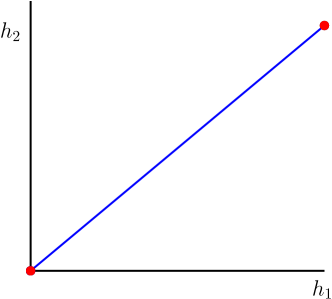
Figure 3. A pictorial explanation of the metric completion $\widehat{\mathcal{S}}_{3}$.

References

- [1] T. Aougab, M. Clay, and Y. Rieck, Thermodynamic metrics on outer space, Ergodic Theory Dynam. Systems, 43 (2023), pp. 729–793.
- [2] P. Blanchard, R. Devaney, and L. Keen, The dynamics of complex polynomials and automorphisms of the shift, Invent. Math., 104 (1991), pp. 545–580.
- [3] B. Branner and J. Hubbard, The iteration of cubic polynomials. I. The global topology of parameter space, Acta Math., 160 (1988), pp. 143–206.
- [4] , The iteration of cubic polynomials. II. Patterns and parapatterns, Acta Math., 169 (1992), pp. 229–325.
- [5] M. Bridgeman, Hausdorff dimension and the Weil-Petersson extension to quasifuchsian space, Geom. Topol., 14 (2010), pp. 799–831.
- [6] M. Bridgeman and E. Taylor, An extension of the Weil-Petersson metric to quasi-Fuchsian space, Math. Ann., 341 (2008), pp. 927–943.
- [7] D. Calegari, Sausages, arXiv:2108.12653.
- [8] , Sausages and butcher paper, in Recent progress in mathematics, vol. 1 of KIAS Springer Ser. Math., Springer, Singapore, [2022] ©2022, pp. 155–200.
- [9] L. DeMarco, Combinatorics and topology of the shift locus, in Conformal dynamics and hyperbolic geometry, vol. 573 of Contemp. Math., Amer. Math. Soc., Providence, RI, 2012, pp. 35–48.
- [10] L. DeMarco and C. McMullen, Trees and the dynamics of polynomials, Ann. Sci. Éc. Norm. Supér. (4), 41 (2008), pp. 337–382.
- [11] L. DeMarco and K. Pilgrim, Critical heights on the moduli space of polynomials, Adv. Math., 226 (2011), pp. 350–372.
- [12] , Hausdorffization and polynomial twists, Discrete Contin. Dyn. Syst., 29 (2011), pp. 1405–1417.
- [13] , Polynomial basins of infinity, Geom. Funct. Anal., 21 (2011), pp. 920–950.
- [14] , The classification of polynomial basins of infinity, Ann. Sci. Éc. Norm. Supér. (4), 50 (2017), pp. 799–877.
- [15] L. DeMarco and A. Schiff, Enumerating the basins of infinity of cubic polynomials, J. Difference Equ. Appl., 16 (2010), pp. 451–461.
- [16] A. Douady and J. Hubbard, Itération des polynômes quadratiques complexes, C. R. Acad. Sci. Paris Sér. I Math., 294 (1982), pp. 123–126.
- [17] L. Goldberg, On the multiplier of a repelling fixed point, Invent. Math., 118 (1994), pp. 85–108.
- [18] Y. He and H. Nie, A riemannian metric on hyperbolic components, to appear Math. Res. Lett.
- [19] O. Ivrii, The geometry of the weil-petersson metric in complex dynamics, to appear Trans. Amer. Math. Soc.
- [20] L. Kao, Pressure type metrics on spaces of metric graphs, Geom. Dedicata, 187 (2017), pp. 151–177.
- [21] J. Kiwi, Combinatorial continuity in complex polynomial dynamics, Proc. London Math. Soc. (3), 91 (2005), pp. 215–248.
- [22] C. McMullen, Thermodynamics, dimension and the Weil-Petersson metric, Invent. Math., 173 (2008), pp. 365–425.
- [23] M. Pollicott and R. Sharp, A Weil-Petersson type metric on spaces of metric graphs, Geom. Dedicata, 172 (2014), pp. 229–244.
- [24] B. Xu, Incompleteness of the pressure metric on the Teichmüller space of a bordered surface, Ergodic Theory Dynam. Systems, 39 (2019), pp. 1710–1728.