Secondary-Structure Phase Formation for Semiflexible Polymers
by Bifurcation in Hyperphase Space

Abstract

Canonical analysis has long been the primary analysis method for studies of phase transitions. However, this approach is not sensitive enough if transition signals are too close in temperature space. The recently introduced generalized microcanonical inflection-point analysis method not only enables the systematic identification and classification of transitions in systems of any size, but it can also distinguish transitions that standard canonical analysis cannot resolve. By applying this method to a generic coarse-grained model for semiflexible polymers, we identify a mixed structural phase dominated by secondary structures such as hairpins and loops that originates from a bifurcation in the hyperspace spanned by inverse temperature and bending stiffness. This intermediate phase, which is embraced by the well-known random-coil and toroidal phases, is testimony to the necessity of balancing entropic variability and energetic stability in functional macromolecules under physiological conditions.

I Introduction

In recent years, substantial research interest has been dedicated to applications in microbiology and nanotechnology on microscopic and mesoscopic scales, where surface effects can not be ignored. Different aspects of biomolecules have been studied extensively. As biomolecules fold into specific structures to perform biological functions in living cells, the computational modeling of these biopolymers, with the advantage of more precise control compared to experiments, has been a crucial way to study structural transitions, which furthermore leads to applications in many areas, e.g., drug discovery and design [1, 2, 3, 4]. Depending on the objective, biopolymer models with different degrees of complexity have been introduced. All-atom simulations provide high resolution for studies of local structure dynamics, but this comes at a very high computational cost and only a limited timescale can be covered [5, 6]. In addition, all-atom simulations often require $\mathcal{O}(10^{3})$ mostly empirical “force field” parameters.

On the other hand, coarse-grained models enable extensive studies of polymer systems at far less computational cost as less relevant degrees of freedom are integrated out. The underlying atomic interactions are replaced by effective interactions between monomers. Extending the coarse-graining procedure further, a monomer can also represent an entire chemical group of atoms or even sections of repeating structures or subunits. Moreover, coarse-grained modeling allows for the systematic study of specific aspects and thus provides a generic insight into the macroscopic properties that are not limited to specific biomolecules [7]. This is the approach we pursue in this study.

DNA, RNA, and proteins can be considered semiflexible polymers, which are characterized by their bending stiffness or finite persistence length. Moreover, bending stiffness has a sigificant impact on biological functions and processes. It helps DNA pack in an organized way for efficient translation and transcription processes [8]. This is important as the length of DNA is very long compared to the size of the cell nucleus it resides in. It is also known that RNA stiffness can affect the self-assembly of virus particles [9].

One of the simplest semiflexible polymer models is the well-known Kratky-Porod or wormlike-chain model [10], which has been successfully used in studies of structural and dynamic properties of semiflexible polymers. However, the lack of self-interactions in this model does not allow for the study of structural phase transitions. Therefore, coarse-grained polymers models with monomer-monomer interaction have been employed to study the phase behavior of semiflexible polymers [11, 12, 13, 14, 15, 16, 17, 18, 19, 20, 21], usually by means of conventional canonical statistical analysis. In this context, it is important to note that biological systems are finite in nature and finite-size scaling is not a generally applicable approach to study the structural phase behavior of these systems. Also, results obtained by canonical statistical analysis are often inconsistent and ambiguous for finite systems. Therefore, it is certainly beneficial to explore other approaches. One candidate is the recently introduced generalized microcanonical inflection-point analysis method that provides a systematic and consistent approach to phase transitions in systems of any size [22].

In this paper, we employ this statistical analysis method to systematically investigate structural transitions for a generic coarse-grained semiflexible polymer model [20]. Section II describes the model, the simulation techniques, and the microcanonical inflection-point analysis method. This is followed by the discussion and comparison of canonical and microcanonical results in Section III. Finally, the paper is concluded by a summary in Section IV.

II Models and Methods

II.1 Coarse-grained Semiflexible Polymer Model

For our study, we use a generic, self-interacting semiflexible homopolymer model. The total energy of a polymer with $N$ monomers in a conformation $\boldsymbol{X}=\left(\boldsymbol{r}_{1},...,\boldsymbol{r}_{N}\right)$, where $\boldsymbol{r}_{n}$ is the position vector of the $n$th monomer, is composed of contributions from bonded and nonbonded interactions between monomers, along with an energetic bending penalty:

$$E(\boldsymbol{X})=\sum_{n}V_{\mathrm{b}}(r_{n\,n+1})+\sum_{n<m+1}V_{\mathrm{nb}}(r_{nm})+\sum_{k}V_{\mathrm{bend}}(\theta_{k}).$$ (1)

Here $r_{nm}=|\boldsymbol{r}_{n}-\boldsymbol{r}_{m}|$ is the distance between monomers $n$ and $m$, and $\theta_{k}$ is the bond angle between two adjacent bonds.

For the interactions between nonbonded monomers, we employ the standard 12-6 Lennard-Jones (LJ) potential

$$V_{\mathrm{LJ}}(r)=4\epsilon_{\mathrm{LJ}}\left[\left(\dfrac{\sigma}{r}\right)^{12}-\left(\dfrac{\sigma}{r}\right)^{6}\right],$$ (2)

where $r$ is the monomer-monomer distance, $\sigma=2^{-1/6}r_{0}$ is the van der Waals distance associated with the potential minimum at $r_{0}$, and $\epsilon_{\mathrm{LJ}}$ is the energy scale. For computational efficiency, we introduce a cutoff at $r_{c}=2.5\sigma$. Shifting the potential by the constant $V_{\mathrm{shift}}\equiv V_{\mathrm{LJ}}(r_{c})$ avoids a discontinuity at $r_{c}$. Thus, the potential energy of nonbonded monomers is given by

$$V_{\mathrm{nb}}(r)=\begin{cases}V_{\mathrm{LJ}}(r)-V_{\mathrm{shift}},&r<r_{c},\\ 0,&\text{otherwise.}\end{cases}$$ (3)

The interaction between bonded monomers is modeled by a combination of the Lennard-Jones potential and the finitely extensible nonlinear elastic (FENE) potential:

$$V_{\mathrm{b}}(r)=V_{\mathrm{FENE}}(r)+V_{\mathrm{LJ}}(r)-V_{\mathrm{shift}},$$ (4)

where the same parameter values of $V_{\mathrm{LJ}}(r)$ are chosen as for nonbonded monomer-monomer interactions. The FENE potential is given by [23, 24, 25]:

$$V_{\mathrm{FENE}}(r)=-\frac{1}{2}KR^{2}\mathrm{ln}\left[1-\left(\frac{r-r_{0}}{R}\right)^{2}\right].$$ (5)

The parameters are fixed to standard values $R=(3/7)r_{0}$ and $K=(98/5)\epsilon_{\mathrm{LJ}}/r_{0}^{2}$ [26] and the bond length $r$ is restricted to fluctuations within the range $[r_{0}-R,r_{0}+R]$. With these parameters, the minimum of $V_{\mathrm{b}}$ is located at $r_{0}$.

To model bending strength, an additional standard potential is introduced. Any deviation of bond angle $\theta$ from the reference angle $\theta_{0}$ between neighboring bonds is subject to an energy penalty of the form:

$$V_{\mathrm{bend}}(\theta)=\kappa\left[1-\cos(\theta-\theta_{0})\right].$$ (6)

The parameter $\kappa\geq 0$ controls the stiffness of the polymer chain. For $\kappa=0$, the model describes flexible polymers [27]. In this study, we chose $\theta_{0}=0$. Therefore, any deviation from the straight chain is energetically unfavorable for $\kappa>0$.

In simulations and statistical analysis of the results, we set $k_{\mathrm{B}}=1$ (Boltzmann constant), $\epsilon_{\mathrm{LJ}}=1$, and $r_{0}=1$. The flexible chain with $N=55$ monomers has already been studied extensively in the past [27] and serves as the reference for the comparison with the semiflexible model. This chain length is sufficiently short to recognize finite-size effects but long enough for the polymer to form stable phases. The results we obtained for this polymer have also been verified for chains with up to $100$ monomers.

II.2 Replica-exchange Simulations of Semiflexible Polymers

The density of states of a system is a core quantity for the microcanonical inflection-point analysis. However, its precise estimation is challenging for complex systems, even with modern computer systems and advanced simulation techniques. For our study, we employed an extended version of replica-exchange Monte Carlo (parallel tempering) [28, 29, 33, 30, 31, 32]. In contrast to simulating the system at fixed temperature, as it is done in conventional Metropolis sampling, parallel tempering has been shown to reach equilibrium faster in simulations at low temperatures [34, 35, 36, 37, 38]. Parallel tempering is a generalized-ensemble method; the microstate probability distribution is governed by the product of Boltzmann factors at all simulation temperatures. It samples the entire state space much more effectively than an ordinary Metropolis Monte Carlo method, which simulates an actual canonical ensemble at a single simulation temperature. The improved performance of parallel tempering is achieved by occasional exchanges of the conformations (replicas) between Metropolis simulation threads running at different temperatures.

Replicas of the system are simulated at different inverse thermal energies $\beta_{i}\in[\beta_{{\min}},\beta_{{\max}}]$, with $i=1,2,\dots,I$, where $I$ is the total number of threads. Here, $\beta=1/k_{\mathrm{B}}T_{\mathrm{can}}$, where $T_{\mathrm{can}}$ is the canonical heat-bath temperature. One obvious advantage of this algorithm is that it can simulate the system under different conditions simultaneously. At each temperature, Metropolis sampling is performed with the acceptance probability:

$$P(\boldsymbol{X}\to\boldsymbol{X}^{\prime})={\min}\left[1,\sigma(\boldsymbol{X},\boldsymbol{X}^{\prime})\omega(\boldsymbol{X},\boldsymbol{X}^{\prime})\right],$$ (7)

where $\omega(\boldsymbol{X},\boldsymbol{X}^{\prime})=\exp\{-\beta[E(\boldsymbol{X}^{\prime})-E(\boldsymbol{X})]\}$ and $\sigma(\boldsymbol{X},\boldsymbol{X}^{\prime})$ is the ratio of forward and backward selection probabilities, which are usually not identical for composite moves such as bond-exchange updates [39]. We also used displacement updates [40], crankshaft rotations [41], and pivot rotations [7] to alter polymer conformations.

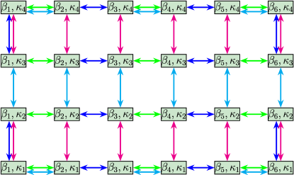
Figure 1: Illustration of the extended replica-exchange Monte Carlo scheme in the combined parameter space of six inverse temperatures $\beta_{1},\ldots,\beta_{6}$ and four bending stiffness values $\kappa_{1},\ldots,\kappa_{4}$. Each node $(i,j)$ represents a simulation thread with a parameter combination of $(\beta_{i},\kappa_{j})$. The four exchange directions, which are chosen randomly from a uniform distribution, are colored differently. The additional exchanges at edge and corner nodes provide for the conservation of replica flows. In our actual simulations, typical grids contained $60\times 4$ parameters in this space.

In our parallel tempering simulations an exchange between the replica with conformation $\boldsymbol{X}$ at inverse temperature $\beta_{i}$ and the replica in state $\boldsymbol{X}^{\prime}$ at $\beta_{j}$ is proposed after $3000$ sweeps (here a sweep corresponds to $N=55$ Monte Carlo updates). The exchange probability is given by

$$a(\boldsymbol{X}\leftrightarrow\boldsymbol{X}^{\prime};\beta_{i},\beta_{j})={\min}\left(1,e^{(\beta_{i}-\beta_{j})(E(\boldsymbol{X})-E(\boldsymbol{X}^{\prime}))}\right).$$ (8)

For the selection of temperature sets that enable efficient exchange between replicas, we found the combination of the geometric and energy methods [42, 43] most reasonable. In these methods, short runs with geometric temperature sets at fixed temperature limits $\beta_{\min}$, $\beta_{\max}$, and number of threads $I$ are performed. The temperature for the simulation thread $i$ is initialized as $\beta_{i}=\beta_{\min}G^{i-1}$, where $G=\left(\beta_{\max}/\beta_{\min}\right)^{1/(I-1)}$. Then the temperatures are adjusted by inserting the estimated average energies in Eq. (8) to get uniform expected exchange probabilities (among all temperature points). For this study, we used the following parameters: $\beta_{\min}=0.25$, $\beta_{\max}=50$, and $I=60$. In typical simulations, up to $10^{9}$ sweeps were performed.

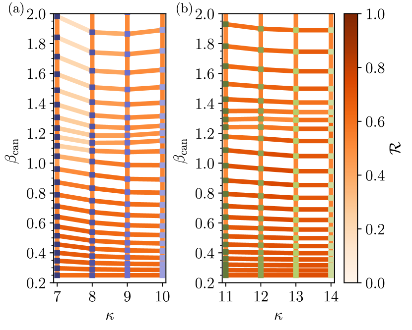
Figure 2: Color-coded replica-exchange acceptance rates of parallel tempering simulations in the combined space of inverse temperature and bending stiffness for (a) for $\kappa=7,8,9,10$ and (b) for $\kappa=11,12,13,14$ between simulation threads (squares) in parameter space. The darker the line color the higher the acceptance rate.

Even though advanced updates were used in our implementation of parallel tempering, the simulation dynamics at low temperatures was still too slow and equilibrium rarely reached. Therefore, we expanded the exchange of replicas to the combined parameter space of simulation temperature and bending stiffness for increased efficiency [12, 17]. For this purpose, the system energy is decoupled,

$$E(\boldsymbol{X})=E_{0}(\boldsymbol{X})+\kappa E_{1}(\boldsymbol{X}),$$ (9)

where $E_{0}(\boldsymbol{X})=\sum_{n}V_{\mathrm{b}}(r_{n\,n+1})+\sum_{n<m+1}V_{\mathrm{nb}}(r_{nm})$ and $E_{1}(\boldsymbol{X})=\sum_{k}\left[1-\cos\theta_{k}\right]$. Consequently, the exchange probability of replica $\boldsymbol{X}$ with bending stiffness $\kappa_{i}$ at inverse temperature $\beta_{i}$ and replica $\boldsymbol{X}^{\prime}$ with bending stiffness $\kappa_{j}$ at inverse temperature $\beta_{j}$ is given by

$$P_{\mathrm{ext}}=\mathrm{min}\left(\exp\left[(\Delta\beta\Delta E_{0})+\Delta(\beta\kappa)\Delta E_{1}\right],1\right).$$ (10)

Here $\Delta\beta=\beta_{i}-\beta_{i+1}$ and $\Delta(\beta\kappa)=\beta_{i}\kappa_{i}-\beta_{i+1}\kappa_{i+1}$. The simulation setup is illustrated in Fig. 1.

In this study, we found $\Delta\kappa=1$ is a sufficient spacing for the range of $\kappa$ values studied. Additional intermediate $\kappa$ values were added, where a finer resolution was needed. In this region of bending stiffnesses, we first simulated two sets of four $\kappa$ values each, $\{7,8,9,10\}$ and $\{11,12,13,14\}$, where $60$ $\kappa-$dependent temperatures, adjusted for parallel tempering, are used for each $\kappa$ value. On occasion, we then also included additional $\kappa$ values to resolve more details of phase behavior in particularly interesting regions of the $\beta-\kappa$ hyperphase diagram.

Combining the energy histograms obtained at different temperatures at fixed $\kappa$ values, the multi-histogram reweighting method [29, 44] yielded an improved estimator for the density of states $g(E)$ that covers the entire energy range at fixed bending stiffness. For further analysis, the Bézier method [45, 46, 7] was used to smooth the microcanonical entropy curves $S(E)=k_{\mathrm{B}}\ln g(E)$ and to calculate its derivatives in preparation of the subsequent microcanonical inflection-point analysis.

In order to assess the performance of the extended parallel-tempering simulation method, we estimated the replica-exchange acceptance rates $\mathcal{R}$. The results are shown in Fig. 2 for two different $\kappa$ ranges. The red color shade encodes the value of $\mathcal{R}$. As we see, all pairs of connected simulation threads (marked by squares) exhibit very good replica-exchange behavior. For the most part, the extensive parameter tuning for $\beta_{\mathrm{can}}$ kept exchange rates in the optimal $0.3<\mathcal{R}<0.7$ range. However, we also observe distinct differences. Whereas the exchange rates are rather uniform for the larger $\kappa$ set as shown in Fig 2(b), the obviously reduced exchange rates between $\kappa=7$ and $\kappa=8$ for inverse temperatures $\beta_{\mathrm{can}}>1.1$ suggest that the system behavior might qualitatively change for $\kappa=7$ and $\kappa=8$, hinting at a possible phase transition in this region of parameter space. This will be investigated in greater detail later by means of microcanonical inflection-point analysis.

Figure 3 shows the quantitative inverse-temperature dependence of $\mathcal{R}$ for selected $\kappa$ values. Again, carefully choosing the inverse simulation temperatures $\beta_{\mathrm{can}}$ establishes almost uniform exchange rates as desired. However, we also observe a major fluctuation in all cases, which shifts toward higher inverse temperatures as $\kappa$ is increased, from $\beta_{\mathrm{can}}\approx 1.15$ for $\kappa=7.5$ to $\beta_{\mathrm{can}}\approx 1.6$ for $\kappa=16$. Typically, large deviations in the exchange rates from a uniform distribution can be associated with phase transitions, which, as we will see, is indeed the case here, too.

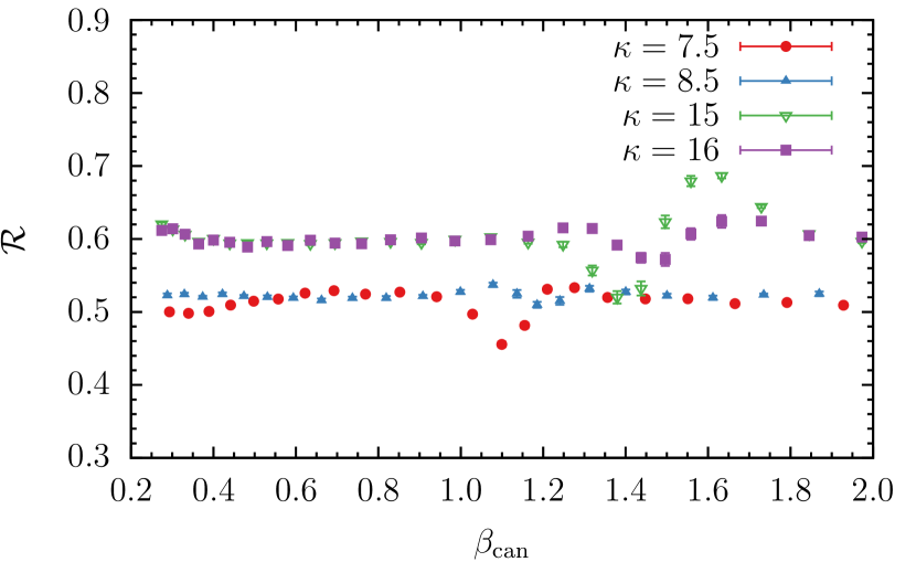
Figure 3: Measured replica-exchange acceptance rates for $\kappa=7.5,8.5,15,16$ in inverse-temperature space.

II.3 Generalized Microcanonical Inflection-point Analysis

The generalized inflection-point analysis method [22] for the systematic identification and classification of transitions in systems of any size combines microcanonical thermodynamics [47] and the principle of minimal sensitivity [48, 49]. It has already led to novel insights into the nature of phase transitions. Even the Ising model, which has been excessively studied for almost a century, possesses a more complex phase structure than previously known [50, 51, 52]. This method has also been employed to particle aggregation [53], self-assembly kinetics in macromolecular systems [54], and in studies of the general geometric and topological foundation of transitions in phase space [55, 56, 57, 58]. It motivated the further investigation of higher-order derivatives of the Boltzmann microcanonical entropy with an additional conserved quantity [59] and has even been used as justification for pattern recognition criteria in computer science [60].

It is important to note that the attribute “microcanonical” has only historical reasons. The analysis method used here has nothing to do with the microcanonical ensemble. The system energy $E$ is not constant. In fact, the density of states, $g(E)$, is a function of energy and it can also be used to calculate energetic “canonical” averages.

Microcanonical statistical analysis is based on the assumption that entropy $S$ and system energy $E$ control the phase behavior of any system. The microcanonical Boltzmann entropy $S(E)=k_{\mathrm{B}}\ln g(E)$ relates these quantities to each other. If the system does not experience phase transitions, the entropy curve $S(E)$ and its derivatives exhibit well-defined concave or convex monotony. However, phase transitions in the system will alter the monotonic behavior, even for finite systems.

From the canonical statistical analysis of first- and second-order transitions, it is known that entropy and/or internal energy $\langle E\rangle$ rapidly change (or are most sensitive), if the heat-bath temperature $T_{\mathrm{can}}$ is varied near the transition point. It can also be interpreted as the temperature change being least sensitive to a change of the internal energy near the transition point.

This behavior corresponds to the least-sensitive dependency of microcanonical quantities in the space of system energies. Thus, a phase transition causes a least-sensitive inflection point in the microcanonical entropy or its derivatives. Therefore, an inflection point can be associated with an extremum in the next-higher derivative at the transition energy, which simplifies the precise identification of the transition point. By systematically analyzing these alterations, different types of transitions can be classified.

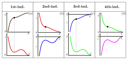
Figure 4: Sketch of independent transitions up to fourth order as defined in the microcanonical inflection-point analysis method. (a) A first-order independent transition is characterized by a least-sensitive inflection point in $S(E)$, which corresponds to a positive minimum in $\beta=dS/dE$. (b) For a second-order transition, the inflection point in $\beta$ is associated with a negative maximum in $\gamma=d^{2}S/dE^{2}$. (c) An inflection point in $\gamma$ defines a third-order transition and $\delta=d^{3}S/dE^{3}$ exhibits a positive minimum. (d) A fourth-order transition possesses an inflection point in $\delta$ and $\epsilon=d^{4}S/dE^{4}$ a negative maximum.

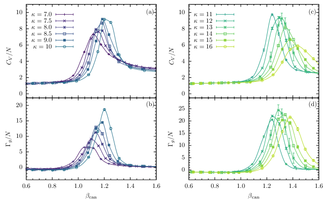
Figure 5: Thermal fluctuations of (a) energy (heat capacity $C_{V}=d\langle E\rangle/dT_{\mathrm{can}}$) and (b) square radius of gyration ($\Gamma_{g}=d\langle R^{2}_{\mathrm{gyr}}\rangle/dT_{\mathrm{can}}$), plotted as functions of $\beta_{\mathrm{can}}$ at selected values of the bending stiffness in the range $7\leq\kappa\leq 10$. (c), (d) Same for examples in the interval $11\leq\kappa\leq 16$.

In this scheme, a first-order transition in $S(E)$ is signaled by a least-sensitive inflection point at transition energy $E_{\mathrm{tr}}$. Therefore, the first derivative, i.e., the inverse microcanonical temperature $\beta(E)\equiv dS/dE$, forms a backbending region as shown in Fig. 4(a) that possesses a positive-valued minimum in $\beta(E)$ at $E_{\mathrm{tr}}$,

$$\beta(E_{\mathrm{tr}})=\dfrac{dS(E)}{dE}\bigg{|}_{E=E_{\mathrm{tr}}}>0.$$ (11)

Similarly, if there is a least-sensitive inflection point in $\beta(E)$, the phase transition is classified as a second-order transition. As shown in Fig. 4(b), the derivative of $\beta(E)$ has a negative-valued peak at the transition energy $E_{\mathrm{tr}}$,

$$\gamma(E_{\mathrm{tr}})=\dfrac{d^{2}S(E)}{dE^{2}}\bigg{|}_{E=E_{\mathrm{tr}}}<0.$$ (12)

This approach can be generalized to any order. Therefore, for a transition of odd order $(2k-1)$ ($k$ is a positive integer), the $(2k-1)$th derivative of $S(E)$ possesses a positive-valued minimum,

$$\dfrac{d^{(2k-1)}S(E)}{dE^{(2k-1)}}\bigg{|}_{E=E_{\mathrm{tr}}}>0,$$ (13)

and a transition of even order $2k$ is characterized by a negative-valued peak in the $2k$th derivative,

$$\dfrac{d^{2k}S(E)}{dE^{2k}}\bigg{|}_{E=E_{\mathrm{tr}}}<0.$$ (14)

We call this transition type an independent phase transition. These turn into the known thermodynamic phase transitions in the thermodynamic limit of infinitely large systems. However, this terminology implies that there is another transition type, dependent transitions [22]. A dependent transition is inevitably associated with an independent transition and it is located in the disordered phase closest to the independent transition. Therefore a dependent transition can be interpreted as precursor of the independent transition it coexists with. Although dependent transitions are less common than independent transitions (only few independent transitions seem to have a dependent companion), they can provide valuable insights into the general nature of transition behavior in complex systems. In the microcanonical inflection-point study of the two-dimensional Ising model, a third-order dependent transition, associated with the well-known critical transition, was identified [52]. It was found to be caused by a collective preordering of spins in the paramagnetic phase. In our study of the phase behavior of semiflexible polymers, dependent transitions were not found, though.

III Bifurcation in the Hyperphase Diagram of Semiflexible Polymers

In the following we analyze the transition behavior of semiflexible polymers from both canonical and microcanonical perspectives. For this purpose we distinguish the canonical inverse heat-bath temperature $\beta_{\mathrm{can}}$ as a thermodynamic state variable from the microcanonical temperature $\beta(E)$, which is a system property.

III.0.1 Canonical Statistical Analysis

Canonical response quantities, such as heat capacity $C_{V}=d\langle E\rangle/dT_{\mathrm{can}}$ and fluctuations of the square radius of gyration, $\Gamma_{g}=d\langle R^{2}_{\mathrm{gyr}}\rangle/dT_{\mathrm{can}}$, are shown in Fig. 5 as functions of $\beta_{\mathrm{can}}$ for a broad range of bending parameter values. For $7\leq\kappa\leq 10$ [Fig. 5(a)], we find that peak values of $C_{V}$ increase for larger bending stiffness. The peak locations shift to larger inverse transition temperatures. The same trend is observed for the peaks in the fluctuations of the square radius of gyration, shown in Fig. 5(b). In fact, these signals are extrapolations of the $\Theta$ collapse transition, well-known from flexible polymers ($\kappa=0$), into the nonzero $\kappa$ regime.

However, surprisingly, a different trend is observed for the heat capacities in the range $11\leq\kappa\leq 16$ [Fig. 5(c)]. The peak values consistently decrease and the peaks broaden again for larger $\kappa$ values. The peak values of the fluctuations of the radius gyration do not keep increasing either. It is important to note that only one major peak is found in these quantities that still suggests a single collapse transition with enhanced thermal activity between entropically favored wormlike chains at higher temperatures and energetically more ordered structures at lower temperatures. As it will turn out later in the structural analysis, this is an incomplete interpretation. Canonical statistical analysis averages out vital information.

Also note the typical ambiguity in the canonical analysis for finite systems. As it can be seen in Fig. 5, peaks in the energetic and structural fluctuations locate the transition points at different temperatures at any given $\kappa$ value. Therefore, in the following, we employ a different analysis approach that helps dissolve the canonical ambiguities in this interesting parameter range for semiflexible polymers and provides a quite clear picture of the actual transition behavior of the system.

III.0.2 Microcanonical Inflection-Point Analysis

Figure 6 nicely illustrates the relationship between inverse temperature and energy in both canonical and microcanonical statistical analysis. The canonical expectation value of the energy $\langle E\rangle(\beta_{\mathrm{can}})$ averages out all fluctuations in system energy $E$ and $\beta_{\mathrm{can}}(\langle E\rangle)$ (blue solid curve) exhibits only a single inflection point, indicating a single transition. In contrast, the microcanonical curve $\beta(E)$ (red dashed curve) reveals two (first-order) transition signals instead in this energy region. The shaded area represents the canonical standard deviation or fluctuation range (which corresponds to the heat capacity). It completely consumes the hierarchical microcanonical transition signals and, therefore, we conclude that the canonical statistical approach is not sufficiently sensitive for the analysis of intricate transition behavior in finite systems.

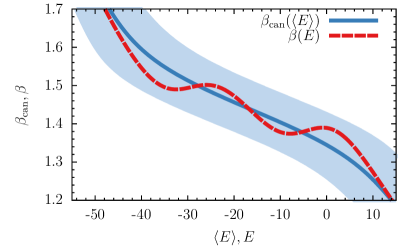
Figure 6: Canonical and microcanonical results for the relationship between inverse temperatures and energies [$\beta_{\mathrm{can}}(\langle E\rangle)$ and $\beta(E)$, respectively] for the semiflexible 55-mer at $\kappa=16$. The shaded area is the standard deviation of the system energy $\sigma(E)$, which represents the thermal fluctuations of the system energy $E$ at the corresponding inverse heat-bath temperature $\beta_{\mathrm{can}}$.

Consequently, we now perform a systematic microcanonical inflection-point analysis. The microcanonical entropy and its derivatives up to second order in the collapse transition region are shown in Figure 7 as functions of the reduced energy $\Delta E^{(\kappa)}=E-E_{\mathrm{min}}^{(\kappa)}$, where $E_{\mathrm{min}}^{(\kappa)}$ is the putative ground-state energy found for a polymer with bending stiffness $\kappa$.

The entropy $S$ does not possess any least-sensitive inflection point in this energy region for $\kappa=7$. However, we identified a least-sensitive inflection point in the $\beta$ curve at $\Delta E^{(\kappa)}\approx 162$. According to our microcanonical inflection-point classification scheme, we consider it an independent second-order transition. It corresponds to a negative maximum in the next-higher derivative, $\gamma(E)$. Similar to chains with bending stiffness $\kappa\leq 6$, only this single second-order transition occurs in this temperature region.

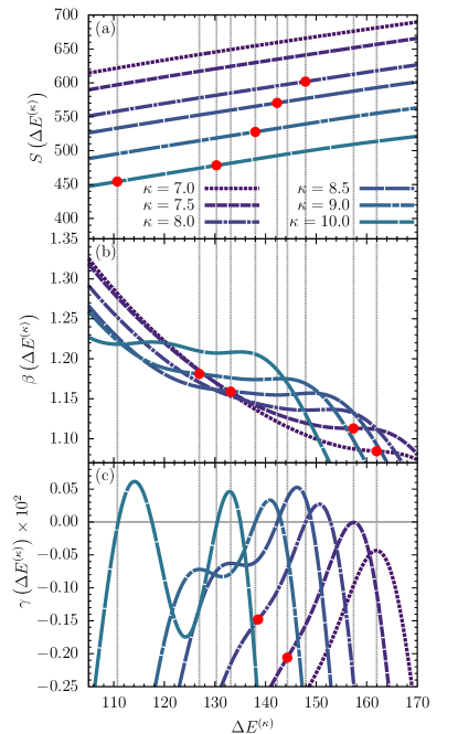
Figure 7: (a) Microcanonical entropy $S$ and its derivatives (b) $\beta=dS/dE$, and (c) $\gamma=d\beta/dE$ for semiflexible polymers with $\kappa=7.0,\dots,10.0$, plotted as functions of the reduced energy $\Delta E^{(\kappa)}$. Least-sensitive inflection points are marked by dots and transition energies are indicated by dotted lines.

For slightly increased bending stiffness $\kappa=7.5$, surprisingly, least-sensitive inflection points are identified in both $\beta$ and $\gamma$, in contrast to the expectation of a single transition point from the canonical analysis. One inflection point in $\beta$ is located at $\Delta E^{(\kappa)}\approx 158$ and another emerges at the lower energy $\Delta E^{(\kappa)}\approx 144$ in $\gamma$, suggesting an independent third-order transition besides the second-order transition.

At the bending stiffness $\kappa=8.0$, an inflection point at $\Delta E^{(\kappa)}\approx 148$ is found in the entropy curve and, thus, corresponds to an independent first-order transition, and associated with it is a positive-valued minimum in $\beta$. This indicates that the extension of the second-order collapse transition known from flexible polymers develops into a first-order transition, whereas the other inflection point in $\gamma$ at $\Delta E^{(\kappa)}\approx 138$ corresponds to a third-order transition.

For $\kappa=8.5$ and $\kappa=9.0$, least-sensitive inflection points show up in the entropy curves at $\Delta E^{(\kappa)}\approx 142$ and $\Delta E^{(\kappa)}\approx 138$, respectively. Therefore, these transitions are classified as first-order transitions. Interestingly, identified by the least-sensitive inflection points in $\beta$, the transitions at energies $\Delta E^{(\kappa)}\approx 143$ for $\kappa=8.5$ and $\Delta E^{(\kappa)}\approx 127$ for $\kappa=9.0$, respectively, change to second-order transitions from the third-order signals we found in this transition region for $\kappa=7$ and $\kappa=7.5$.

Strikingly, for $\kappa=10.0$, both least-sensitive inflection points are found in $S$, which are identified best from the two separate positive minima in $\beta$ at $\Delta E^{(\kappa)}\approx 130$ and at $\Delta E^{(\kappa)}\approx 110$. Thus, the new transition branch finally turns into another first-order transition line.

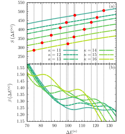
Figure 8: (a) Microcanonical entropy $S$ and its derivative (b) $\beta=dS/dE$ for $\kappa=11,\dots,16$, plotted as functions of $\Delta E^{(\kappa)}$. Dots show the locations of least-sensitive inflection points; dotted lines were drawn at the transition energies.

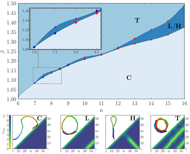
Figure 9: Hyperphase diagram for semiflexible polymers with 55 monomers, parametrized by bending stiffness $\kappa$ and inverse microcanonical temperature $\beta$. Red diamonds mark first-order, blue dots second-order, and purple triangles third-order transitions as identified by microcanonical inflection-point analysis of results obtained in our simulations. Solid transition lines are guides to the eye. Conformations characteristic for the respective phases and their distance maps (lower triangles in the insets) are shown below the phase diagram. We distinguish the following structure types: C: random coils in the wormlike-chain regime, H: hairpins, L: loops, and T: toroids. Monomer labels are ordered from the blue (first monomer) to the red end (last monomer).

Extending the analysis further to bending stiffness values $\kappa=11,\dots,16$, we obtain the results shown in Fig. 8. For each $\kappa$ value, only pairs of least-sensitive inflection points in the entropy curves are found in this energy region. Therefore, these are independent first-order transitions that are clearly signaled by positive minima in the $\beta$ curves. As can be seen in Fig. 8(a), the transition energy difference between the two first-order transitions increases for stiffer chains. For larger bending stiffness values, the difference of the corresponding microcanonical inverse transition temperatures is larger as well. The back-bending features in the $\beta$ curves near the transitions points are more prominent for chains with greater bending stiffness. This is an important result as it shows that the two transition lines that have formed out of the bifurcation point, embrace an entirely new phase and the fact that the first-order transition characteristics become more pronounced means that the phase is getting more stable as $\kappa$ increases in this region of the phase diagram.

The $\beta-\kappa$ hyperphase diagram constructed from the results we obtained by microcanonical inflection-point analysis in the vicinity of the bifurcation point is shown in Fig. 9. The extension of the coil-globule transition line remains intact as a single second-order transition from the flexible case ($\kappa=0$) up to the bifurcation located at about $\kappa=7$ and $\beta=1.08$. Note that, for bending stiffness values $\kappa>7$, transition types on the upper line change from third via second to first order. We have already discussed this transition behavior in the context of the microcanonical analysis. For finite systems, this is a characteristic feature of transition lines branching off a main transition line. Transitions of higher-than-second order are also common in finite systems [22, 27]. Without their consideration, the phase diagram would contain a gap.

In the higher-temperature regime (low $\beta$), the disordered phase C is governed by wormlike random-coil structures. In this regime, entropic effects enable sufficiently large fluctuations that suppress the formation of stable energetic contacts between monomers. For $\kappa\leq 7$, coil structures directly transition into the toroidal phase T upon lowering the temperature (increasing $\beta$). However, more interestingly, the formation of a new stable phase between the random-coil phase C and the toroidal phase T is observed for $\kappa>7$. This phase is characterized by the coexistence of hairpins (H) and loop (L) structures. Therefore, we call it a mixed phase. Wormlike chains fold into hairpins and eventually loops in this transition process. Further cooling leads to another transition into the toroidal phase T.

By analyzing the structures in these phases, we found that they possess unique arrangements of nonbonded monomer-monomer contacts. Therefore, we used distance maps of monomers to characterize these phases. As shown in Fig. 9, the representative conformations as well as their distance maps for each phase are included. The two nonbonded monomers $n$ and $m$ are considered to be in close contact if their distance $r_{nm}<1.2$, but the results are not very sensitive to this choice, as long as counting nonnearest neighbor contacts is avoided. This threshold distance is close to the minimum of the Lennard-Jones potential. Nonbonded monomer pairs in contact are represented by the yellow region in the triangular distance maps shown underneath the conformations. For the extended coil structures, stable contacts of monomers are prevented by thermal fluctuations, and thus they do not exhibit any particular features. In the intermediate phase, the tails of hairpin structures are in contact, with antiparallel orientation. This results in the contact line that is perpendicular to the diagonal in the contact map, which makes it easy to identify these structures. In loops, on the other hand, the tails align with parallel orientation. Consequently, the short contact line is parallel to the diagonal in the contact map. In contrast to loops, toroids try to reduce system energy by forming additional contacts. As a result, a second streak parallel to the diagonal in the contact map accounts for another winding.

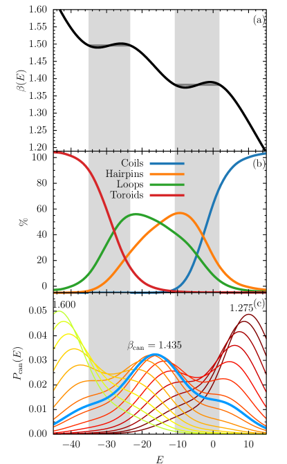
Figure 10: (a) Microcanonical temperature and (b) system energy dependence of frequencies for the different structure types at $\kappa=16$. (c) Canonical energy probability distributions $P_{\mathrm{can}}$ at various inverse thermal energies $\beta_{\mathrm{can}}=1/k_{\mathrm{B}}T_{\mathrm{can}}$.

In order to quantify the population of different structures in each phase and to gain more insights into the transition behavior in this energy range, we have also measured the probabilities for each structure type as functions of the system energy. Detailed results for $\kappa=16$ are presented in Fig. 10. The $\beta$ curve is shown in Fig. 10(a) and the frequencies of the different structure types in Fig. 10(b). The microcanonical Maxwell constructions for $\beta$ in the transition regions define the coexistence regions of first-order transitions. These regions are shaded gray; their widths are a measure for the latent heat. There is a clearly visible energetic gap between the two transitions (the two coexistence regions do not overlap), confirming that the hairpin-loop crossover is a stable intermediate phase. The canonical energy probability distributions $P_{\mathrm{can}}(E)$ shown in Fig. 10(c) for various canonical temperatures support this interpretation. There are two noticeable suppressed regions in the envelope of these curves, each caused by a first-order transition. The locations nicely coincide with the corresponding first-order transition regions we identified by microcanonical inflection-point analysis. Interestingly, the distribution for $\beta_{\mathrm{can}}=1.435$ (blue curve) spans the entire energy range, and the presence of two transitions is only reflected by the two shoulders on either side of the peak. This also helps explain the single peak in the specific heat curve for $\kappa=16$ in Fig. 5(c): The fluctuation range covers the entire energy region of both transitions. Therefore, the two individual transitions cannot be distinguished by the canonical analysis of response quantities.

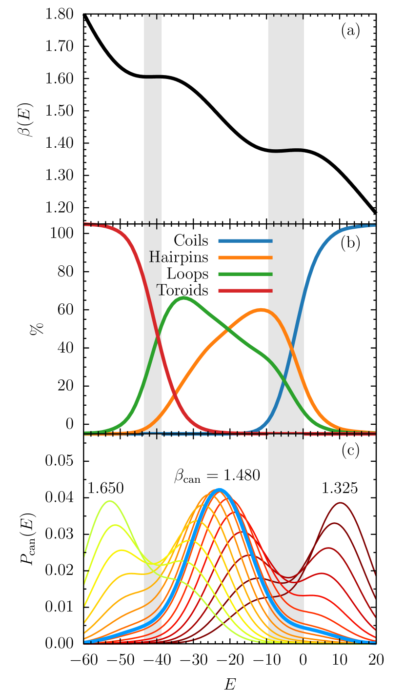
Figure 11: Same as Fig. 10, but for $N=70,\kappa=30$.

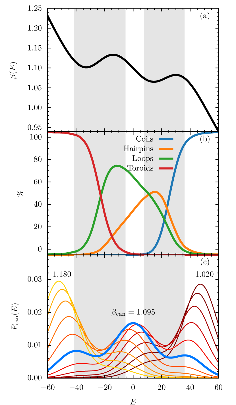
Figure 12: Same as Fig. 10, but for $N=100,\kappa=45$.

At high energies, coil structures dominate the phase behavior. Upon lowering the energy, there are mainly two ways for the extended coils to fold and create tail contacts, parallel and antiparallel. During the ensuing transition, the presence of hairpins with antiparallel tail contacts rapidly increases. These conformations still provide sufficient entropic freedom for the dangling tail, which is already stabilized by van der Waals contacts, however. The loop part of the hairpin helps reduce the stiffness restraint. It is noteworthy that the pure loop structures with parallel tails also significantly contribute to the population, although at a lesser scale in this region. The actual crossover from hairpins to loops happens within the phase. For lower energies in this mixed phase, the population of hairpins decreases, whereas loops take over dominance. Moreover, the energy difference between these two types of structures is sufficiently small for thermal fluctuations to easily convert one structure type to the other by folding the tails back to or away from the loop part. This also explains why there is no phase transition between them. Importantly, even though hairpin and loop structures are irrelevant at very low temperatures, they are biologically significant secondary structure types at finite temperatures. The tail can be easily spliced, contact pair by contact pair, with little energetic effort, which supports essential micromolecular processes on the DNA and RNA level such as transcription and translation. Therefore, it is important to discern the phase dominated by these structures.

Upon further reducing the energy (and therefore also entropy), forming energetically favorable van der Waals contacts becomes the dominant structure formation strategy and loops coil in to eventually form toroids. In contrast to loops, toroidal structures are more ordered and stabilized further by additional energetically favorable attractions between monomers.

To test the robustness of the obtained results, we have also performed selected simulations of semiflexible chains of this generic model with 70 and 100 monomers, essentially yielding the same qualitative results. Most importantly, the bifurcation of the collapse transition line is also observed for these chain lengths. Quantitatively, the bifurcation point is shifted toward higher bending stiffness. For $N=70$, it is located at about $\kappa=20$, whereas it is near $\kappa=40$ for $N=100$. This is expected, of course, as the number of possible energetic contacts scales with the number of monomers, which requires a larger energy penalty to break these contacts. It also helps understand why microbiological structures are not only finite but exist on a comparatively small, mesoscopic length scale. At the physiological scale, structure formation processes of large systems would be much more difficult to control and stabilize. This also means that studying such systems in the thermodynamic limit may not actually aid in understanding physics at mesoscopic scales.

We also analyzed the structure population for the two first-order transitions at these chain lengths. The results for ($N=70,\kappa=30$) and ($N=100,\kappa=45$) are shown in Fig. 11 and Fig. 12, respectively. In both cases the same crossover behavior of hairpins and loops in the intermediate phases as for $N=55$ is observed. The two suppressed regions of canonical energy distribution probabilities are clearly visible as well. These results support the generality of our conclusions for semiflexible polymers on mesoscopic scales.

IV Summary

We employed the microcanonical inflection-point analysis method to study the transition behavior of a generic semiflexible polymer model with self-interactions. The replica-exchange Monte Carlo simulation method, extended to cover both temperature and bending stiffness parameter spaces, was used to obtain highly accurate estimates of the density of states needed for the microcanonical statistical analysis. Advanced structural Monte Carlo updates helped improve the efficiency of our simulations. Least-sensitive inflection points in the microcanonical entropy and its derivatives were used as indicators for the systematic identification and classification of phase transitions.

The coarse-grained semiflexible polymer we mainly studied consists of 55 repetitive units (monomers). This chain has been extensively studied in the flexible limit. Therefore, in this study, we focused on the transition line that extends from the collapse transition point for flexible polymers upon increasing the value of the bending stiffness parameter of the chain. Below a certain threshold, for nonzero bending stiffness, the line separates wormlike-chain coil structures from toroidal conformations. However, remarkably, we find that the line bifurcates at a certain bending strength, which leads to the formation of an intermediate, mixed phase of stable secondary structures such as hairpins and loops. Whereas the extended collapse transition line below the bifurcation point is of second order, the two transitions embracing the novel intermediate phase eventually turn into comparatively strong first-order transitions. In the bifurcation region, the new transition branch starts off with third-order, then second-order, and finally first-order transition behavior for sufficiently large values of the bending stiffness.

It is worth emphasizing that these transition signals are indistinguishable in canonical statistical analysis, where the energetic fluctuations are large enough to envelop both transitions. Therefore, conventional canonical statistical analysis of fluctuations of response quantities was found to be too insensitive to reveal the separate phase of microbiologically important secondary structures.

As detailed structural analysis showed, the mixed intermediate phase is populated by both loop and hairpin structures, which are biologically relevant secondary structures present in DNA and RNA under physiological conditions. These structures are inherently finite in size. Yet, studies of chains with different lengths also confirmed that our results are robust and this intermediate phase is stable.

Our results support the conclusion that biomolecular function is inevitably connected to structural features of segments of macromolecules on mesoscopic scales. For semiflexible polymers, hairpins and loops are the optimal secondary structure types that represent the best compromise of structural stability and variability under thermal conditions. Stability is achieved by reducing energy and variability by increasing entropy. Therefore, biologically relevant functional polymers must be able to adapt to environmental conditions by resisting random energetic fluctuations, but also allowing for structural changes on small energetic scales to ensure predictable functional behavior. Therefore, as our study showed, only semiflexible polymers with sufficient bending stiffness exceeding a certain threshold can form a separate intermediate phase of secondary structures, making them excellent candidates for functional biomolecules.

V Conflicts of Interest

There are no conflicts of interest to declare.

VI Acknowledgment

This study was supported in part by resources and technical expertise from the Georgia Advanced Computing Resource Center (GACRC).

References

- [1] Ferreira, L. G.; Dos Santos, R. N.; Oliva, G.; Andricopulo, A. D. Molecular Docking and Structure-Based Drug Design Strategies. Molecules 2015, 20 (7), 13384-13421.
- [2] Gao, P.; Nicolas, J.; Ha-Duong, T. Supramolecular Organization of Polymer Prodrug Nanoparticles Revealed by Coarse-Grained Simulations. J. Am. Chem. Soc. 2021, 143 (42), 17412-17423.
- [3] Schmidt, T.; Bergner, A.; Schwede, T. Modelling Three-Dimensional Protein Structures for Applications in Drug Design. Drug Discov. Today 2014, 19 (7), 890-897.
- [4] Smiatek, J.; Jung, A.; Bluhmki, E. Towards a Digital Bioprocess Replica: Computational Approaches in Biopharmaceutical Development and Manufacturing. Trends Biotechnol. 2020, 38 (10), 1141-1153.
- [5] Kmiecik, S.; Gront, D.; Kolinski, M.; Wieteska, L.; Dawid, A. E.; Kolinski, A. Coarse-Grained Protein Models and Their Applications. Chem. Rev. 2016, 116 (14), 7898-7936.
- [6] Singh, N.; Li, W. Recent Advances in Coarse-Grained Models for Biomolecules and Their Applications. Int. J. Mol. Sci. 2019, 20 (15), 3774.
- [7] Bachmann, M. Thermodynamics and Statistical Mechanics of Macromolecular Systems; Cambridge University Press, 2014.
- [8] Yuan, C.; Chen, H.; Lou, X. W.; Archer, L. A. DNA Bending Stiffness on Small Length Scales. Phys. Rev. Lett. 2008, 100 (1), 018102.
- [9] Li, S.; Erdemci-Tandogan, G.; van der Schoot, P.; Zandi, R. The Effect of RNA Stiffness on the Self-Assembly of Virus Particles. J. Phys.: Condens. Matter 2018, 30 (4), 044002.
- [10] Kratky, O.; Porod, G. Röntgenuntersuchung Gelöster Fadenmoleküle. Recl. Trav. Chim. Pays-Bas 1949, 68 (12), 1106-1122.
- [11] Seaton, D. T.; Schnabel, S.; Landau, D. P.; Bachmann, M. From Flexible to Stiff: Systematic Analysis of Structural Phases for Single Semiflexible Polymers. Phys. Rev. Lett. 2013, 110 (2), 028103.
- [12] Marenz, M.; Janke, W. Knots as a Topological Order Parameter for Semiflexible Polymers. Phys. Rev. Lett. 2016, 116 (12), 128301.
- [13] Skrbic, T.; Hoang, T. X.; Giacometti, A. Effective Stiffness and Formation of Secondary Structures in a Protein-like Model. J. Chem. Phys. 2016, 145 (8), 084904.
- [14] Wu, J.; Cheng, C.; Liu, G.; Zhang, P.; Chen, T. The Folding Pathways and Thermodynamics of Semiflexible Polymers. J. Chem. Phys. 2018, 148 (18), 184901.
- [15] Wu, J.; Huang, Y.; Yin, H.; Chen, T. The Role of Solvent Quality and Chain Stiffness on the End-to-End Contact Kinetics of Semiflexible Polymers. J. Chem. Phys. 2018, 149 (23), 234903.
- [16] Aierken, D.; Bachmann, M. Comparison of Conformational Phase Behavior for Flexible and Semiflexible Polymers. Polymers 2020, 12, 3013.
- [17] Majumder, S.; Marenz, M.; Paul, S.; Janke, W. Knots Are Generic Stable Phases in Semiflexible Polymers. Macromolecules 2021, 54(12), 5321-5334.
- [18] Walker, C. C.; Fobe, T. L.; Shirts, M. R. How Cooperatively Folding Are Homopolymer Molecular Knots? Macromolecules 2022, 55 (19), 8419-8437.
- [19] Shakirov, T.; Paul, W. Aggregation and Crystallization of Small Alkanes. J. Chem. Phys. 2023, 158 (9), 094905.
- [20] Aierken, D.; Bachmann, M. Stable Intermediate Phase of Secondary Structures for Semiflexible Polymers. Phys. Rev. E 2023, 107 (3), L032501.
- [21] Aierken, D.; Bachmann, M. Impact of Bending Stiffness on Ground State Conformations for Semiflexible Polymers. J. Chem. Phys. 2023, 158 (21), 214905.
- [22] Qi, K.; Bachmann, M. Classification of Phase Transitions by Microcanonical Inflection-Point Analysis. Phys. Rev. Lett. 2018, 120 (18), 180601.
- [23] Bird, R. B.; Armstrong, R. C.; Hassager, O. Dynamics of Polymeric Liquids. Vol. 1: Fluid Mechanics. 1987.
- [24] Kremer, K.; Grest, G. S. Dynamics of Entangled Linear Polymer Melts: A Molecular-dynamics Simulation. J. Chem. Phys. 1990, 92 (8), 5057-5086.
- [25] Milchev, A.; Bhattacharya, A.; Binder, K. Formation of Block Copolymer Micelles in Solution: A Monte Carlo Study of Chain Length Dependence. Macromolecules 2001, 34 (6), 1881-1893.
- [26] Qi, K.; Bachmann, M. Autocorrelation Study of the Transition for a Coarse-Grained Polymer Model. J. Chem. Phys. 2014, 141 (7), 074101.
- [27] Qi, K.; Liewehr, B.; Koci, T.; Pattanasiri, B.; Williams, M. J.; Bachmann, M. Influence of Bonded Interactions on Structural Phases of Flexible Polymers. J. Chem. Phys. 2019, 150 (5), 054904.
- [28] Swendsen, R. H.; Wang, J.-S. Replica Monte Carlo Simulation of Spin-Glasses. Phys. Rev. Lett. 1986, 57 (21), 2607.
- [29] Ferrenberg, A. M.; Swendsen, R. H. New Monte Carlo Technique for Studying Phase Transitions. Phys. Rev. Lett. 1988, 61 (23), 2635.
- [30] Hukushima, K.; Nemoto, K. Exchange Monte Carlo Method and Application to Spin Glass Simulations. J. Phys. Soc. Jpn. 1996, 65 (6), 1604-1608.
- [31] Hukushima, K.; Takayama, H.; Nemoto, K. Application of an Extended Ensemble Method to Spin Glasses. Int. J. Mod. Phys. C 1996, 07, 07, 337-344
- [32] Earl, D. J.; Deem, M. W. Parallel Tempering: Theory, Applications, and New Perspectives. Phys. Chem. Chem. Phys. 2005, 7 (23), 3910.
- [33] Geyer, C. J. Computing Science and Statistics: Proceedings of the 23rd Symposium on the Interface. J. Am. Stat. Assoc. 1991, 156.
- [34] Fiore, C. E. First-Order Phase Transitions: A Study through the Parallel Tempering Method. Phys. Rev. E 2008, 78 (4), 041109.
- [35] Kofke, D. A. Comment on “The Incomplete Beta Function Law for Parallel Tempering Sampling of Classical Canonical System” [J. Chem. Phys. 120, 4119 (2004)]. J. Chem. Phys. 2004, 121 (2), 1167-1167.
- [36] Machta, J. Strengths and Weaknesses of Parallel Tempering. Phys. Rev. E 2009, 80 (5), 056706.
- [37] Machta, J.; Ellis, R. S. Monte Carlo Methods for Rough Free Energy Landscapes: Population Annealing and Parallel Tempering. J. Stat. Phys. 2011, 144 (3), 541-553.
- [38] Predescu, C.; Predescu, M.; Ciobanu, C. V. On the Efficiency of Exchange in Parallel Tempering Monte Carlo Simulations. J. Phys. Chem. B 2005, 109 (9), 4189-4196.
- [39] Schnabel, S.; Janke, W.; Bachmann, M. Advanced Multicanonical Monte Carlo Methods for Efficient Simulations of Nucleation Processes of Polymers. J. Comput. Phys. 2011, 230 (12), 4454-4465.
- [40] Williams, M. J.; Bachmann, M. Significance of Bending Restraints for the Stability of Helical Polymer Conformations. Phys. Rev. E 2016, 93 (6), 062501.
- [41] Austin, K. S.; Marenz, M.; Janke, W. Efficiencies of Joint Non-Local Update Moves in Monte Carlo Simulations of Coarse-Grained Polymers. Comput. Phys. Commun. 2018, 224, 222-229.
- [42] Hukushima, K. Domain-Wall Free Energy of Spin-Glass Models: Numerical Method and Boundary Conditions. Phys. Rev. E 1999, 60 (4), 3606-3613.
- [43] Rozada, I.; Aramon, M.; Machta, J.; Katzgraber, H. G. Effects of Setting Temperatures in the Parallel Tempering Monte Carlo Algorithm. Phys. Rev. E 2019, 100 (4), 043311.
- [44] Kumar, S.; Rosenberg, J. M.; Bouzida, D.; Swendsen, R. H.; Kollman, P. A. The Weighted Histogram Analysis Method for Free-energy Calculations on Biomolecules. I. The Method. J. Comput. Chem. 1992, 13 (8), 1011-1021.
- [45] Bézier, P. Procédé de Définition Numérique Des Courbes et Surfaces Non Mathématiques. Automatisme 1968, 13 (5), 189-196.
- [46] Gordon, W. J.; Riesenfeld, R. F. Bernstein-Bézier Methods for the Computer-Aided Design of Free-Form Curves and Surfaces. J. ACM 1974, 21 (2), 293-310.
- [47] Gross, D. H. E. Microcanonical Thermodynamics: Phase Transitions in ”Small” Systems; World Scientific, 2001.
- [48] Stevenson, P. M. Resolution of the Renormalisation-Scheme Ambiguity in Perturbative QCD. Phys. Lett. B 1981, 100 (1), 61-64.
- [49] Stevenson, P. M. Optimized Perturbation Theory. Phys. Rev. D 1981, 23 (12), 2916-2944.
- [50] Sitarachu, K.; Bachmann, M. Phase Transitions in the Two-Dimensional Ising Model from the Microcanonical Perspective. J. Phys.: Conf. Ser. 2020, 1483, 012009.
- [51] Sitarachu, K.; Zia, R. K. P.; Bachmann, M. Exact Microcanonical Statistical Analysis of Transition Behavior in Ising Chains and Strips. J. Stat. Mech. 2020, 2020 (7), 073204.
- [52] Sitarachu, K.; Bachmann, M. Evidence for Additional Third-Order Transitions in the Two-Dimensional Ising Model. Phys. Rev. E 2022, 106 (1), 014134.
- [53] Trugilho, L. F.; Rizzi, L. G. Microcanonical Characterization of First-Order Phase Transitions in a Generalized Model for Aggregation. J. Stat. Phys. 2022, 186 (3), 40.
- [54] Trugilho, L. F.; Rizzi, L. G. Shape-Free Theory for the Self-Assembly Kinetics in Macromolecular Systems. EPL 2022, 137 (5), 57001.
- [55] Bel-Hadj-Aissa, G.; Gori, M.; Penna, V.; Pettini, G.; Franzosi, R. Geometrical Aspects in the Analysis of Microcanonical Phase-Transitions. Entropy 2020, 22 (4), 380.
- [56] Gori, M.; Franzosi, R.; Pettini, G.; Pettini, M. Topological Theory of Phase Transitions. J. Phys. A: Math. Theor. 2022, 55 (37), 375002.
- [57] Pettini, G.; Gori, M.; Franzosi, R.; Clementi, C.; Pettini, M. On the Origin of Phase Transitions in the Absence of Symmetry-Breaking. Phys. A: Stat. Mech. 2019, 516, 376-392.
- [58] Di Cairano, L.; Capelli, R.; Bel-Hadj-Aissa, G.; Pettini, M. Topological Origin of the Protein Folding Transition. Phys. Rev. E 2022, 106 (5), 054134.
- [59] Bel-Hadj-Aissa, G. High Order Derivatives of Boltzmann Microcanonical Entropy with an Additional Conserved Quantity. Phys. Lett. A 2020, 384 (24), 126449.
- [60] Chaudhuri, A.; Sadek, C.; Kakde, D.; Wang, H.; Hu, W.; Jiang, H.; Kong, S.; Liao, Y.; Peredriy, S. The Trace Kernel Bandwidth Criterion for Support Vector Data Description. Pattern Recognit. 2021, 111, 107662.