Addressing the speed-accuracy simulation trade-off for adaptive spiking neurons

Abstract

The adaptive leaky integrate-and-fire (ALIF) model is fundamental within computational neuroscience and has been instrumental in studying our brains in silico. Due to the sequential nature of simulating these neural models, a commonly faced issue is the speed-accuracy trade-off: either accurately simulate a neuron using a small discretisation time-step (DT), which is slow, or more quickly simulate a neuron using a larger DT and incur a loss in simulation accuracy. Here we provide a solution to this dilemma, by algorithmically reinterpreting the ALIF model, reducing the sequential simulation complexity and permitting a more efficient parallelisation on GPUs. We computationally validate our implementation to obtain over a $50\times$ training speedup using small DTs on synthetic benchmarks. We also obtained a comparable performance to the standard ALIF implementation on different supervised classification tasks - yet in a fraction of the training time. Lastly, we showcase how our model makes it possible to quickly and accurately fit real electrophysiological recordings of cortical neurons, where very fine sub-millisecond DTs are crucial for capturing exact spike timing.

1 Introduction

The surge of progress in artificial neural networks (ANNs) over the last decade has advanced our understanding of the potential computational principles underlying the processing of sensory information [1, 2, 3, 4, 5, 6, 7, 8, 9]. Although these networks architecturally bear a resemblance to the brain [10], they tend to omit a key physiological constraint: the spike. With their increased biological realism, spiking neural networks (SNNs) have shown great promise in bridging the gap between experimental data and computational models. SNNs can be fitted to real neural data [11, 12, 13, 14, 15], or used to simulate the brain, offering a new level of understanding of the complex workings of the nervous system [16, 17, 18, 19]. They also have engineering applications in energy-efficient machine learning [20].

An established class of spiking models in computational neuroscience is the leaky integrate-and-fire (LIF) neuron, with origins dating back to 1907 [21]. Just like in real neurons, input current (resulting from presynaptic input) charges the membrane potential of the model neurons, which then output binary signals (i.e. spikes) as a form of communication (Figure 1a). The adaptive leaky integrate-and-fire (ALIF) model [22] is a modern extension of the LIF. It more closely mimics the biology, capturing a key property of neurons, which is their adaptive firing threshold (i.e. spikes become less frequent in response to a steady input current [23]). ALIF neurons have been shown to accurately fit real neural recordings [11, 22, 24, 25] and to outperform the simpler LIF neurons on various machine learning benchmarks [26, 27, 28, 29].

Despite these modelling advances, a major shortcoming of LIF and ALIF neurons is their slow inference and training times. Unlike real neurons, modelling neuron dynamics involves sequential computation over discretised time. This leads to a problematic trade-off between speed and accuracy when simulating SNNs. A small DT enables accurate modelling of dynamics, but is slow to stimulate and train on computer systems such as GPUs. A large DT obtains less accurate dynamics, but at the benefit of being faster to simulate and train [30] (Figure 1b). This raises the important question of capturing the best of both worlds: is there a way to accelerate the inference and training of spiking LIF and ALIF neurons without sacrificing simulation accuracy?

In this work, we address the speed-accuracy trade-off when simulating and training LIF and ALIF SNNs, and present a solution that is both fast and accurate. We take advantage of a fundamental property of neurons that is sometimes not modelled - the absolute refractory period (ARP). This is a short period of time following spike initiation, during which a neuron cannot fire again. As a result, a neuron can spike at most once within such a period (Figure 1c). We leverage this observation to develop a novel algorithmic reformulation of the ALIF model which reduces the sequential simulation complexity of the standard ALIF algorithm. Specifically, we outline how ALIF recurrent networks can be simulated with a constant sequential complexity $O(1)$ over the ARP simulation length $T_{R}$, and how this approach can be extended to longer simulation lengths to obtain identical dynamics to the standard ALIF network algorithm. Faster simulation and training are theoretically obtained for growing length $T_{R}$, by either employing physiologically plausible ARPs of $\sim 2$ms and decreasing the DT to a very fine value $\sim 0.1$ms (for realistic neural modelling), or setting the DT to a coarser value and adopting larger non-physiological ARPs (for machine learning tasks). Our main contributions are the following:

• We develop a novel algorithmic reformulation of the ALIF model with an $O(T/T_{R})$ - rather than $O(T)$ - sequential complexity, for simulation length $T$ and ARP length $T_{R}$.

• We find that our model achieves substantial inference (up to $40\times$) and training speedup (up to $53\times$) over the standard ALIF SNN for increasing ARP time steps, and find this to hold over different numbers of simulation lengths, batch sizes, number of neurons and layers.

• We demonstrate the feasibility of our model to be trained using surrogate gradient descent, with our accelerated ALIF SNN achieving comparable accuracies to the standard ALIF SNN on temporal spiking classification datasets - yet in a fraction of the training time.

• Finally, we showcase how our ALIF implementation makes it possible to quickly fit real electrophysiological recordings of cortical neurons, where very fine sub-millisecond discretisation steps are important for accurately capturing exact spike timing.

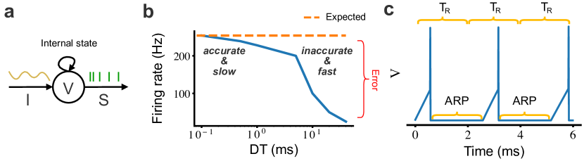
Figure 1: Problem overview. a. Schematic of an ALIF neuron: input current $I$ charges membrane potential $V$ and outputs spikes $S$ if firing threshold is reached (with the neuron’s internal state evolving over time). b. An example of the simulation trade-off problem when simulating a single ALIF neuron with fixed synaptic weights receiving Poisson spike input. The simulation error and the speed grow for increasing discretisation time (DT). c. Observation for our solution: a neuron emits at most a single spike during a simulation span $T_{R}$ equal in length to the neuron’s absolute refractory period (ARP).

2 Background and related work

Standard ALIF model

We introduce the recurrent SNN of ALIF neurons with fixed ARP and latency of recurrent transmission, defined by the following set of equations [26, 31].

$$S_{i}^{(l)}[t] =f(V^{(l)}_{i}[t])=\mathbb{1}_{V^{(l)}_{i}[t]>\theta_{i}^{(l)}[t]}\quad\text{(Output spike)}$$ (1)

$$V^{(l)}_{i}[t] =\big{(}\beta_{i}^{(l)}V^{(l)}_{i}[t-1]+(1-\beta_{i}^{(l)})I_{i}^{(l)}[t]\big{)}\big{(}1-S^{(l)}_{i}[t-1]\big{)}\quad\text{(Membrane potential)}$$ (2)

$$\tilde{I}_{i}^{(l)}[t] =\Big{(}b_{i}^{(l)}+\underbrace{\sum_{j=1}^{N^{(l-1)}}W^{(l)}_{ij}S^{(l-1)}_{j}[t]}_{\text{Feedforward current}}+\underbrace{\sum_{j=1}^{N^{(l)}}W^{\text{rec }(l)}_{ij}S^{(l)}_{j}[t-D]}_{\text{Recurrent current}}\Big{)}\quad\text{(Input current)}$$ (3)

$$I_{i}^{(l)}[t] =\begin{cases}\tilde{I}_{i}^{(l)}[t]&\text{if }C_{i}^{(l)}\geq T_{R}\\ 0&\text{otherwise}\end{cases}\quad\text{(Absolute refractory period)}$$ (4)

$$\begin{split}\theta_{i}^{(l)}[t]&=1+d_{i}^{(l)}a_{i}^{(l)}[t]\\ a_{i}^{(l)}[t]&=p_{i}^{(l)}a_{i}^{(l)}[t-1]+S_{i}^{(l)}[t-1]\end{split}\quad\text{(Adaptation)}$$ (5)

At time $t$, neuron $i$ within layer $l$ (consisting of $N^{(l)}$ neurons) receives input current $I_{i}^{(l)}[t]$ and outputs a binary value $S_{i}^{(l)}[t]\in\{1,0\}$ (i.e. spike or no spike) if a neuron’s membrane potential $V_{i}^{(l)}[t]$ reaches firing threshold $\theta_{i}^{(l)}$ (Equation 1). The evolution of the membrane potential is described by the normalised discretised LIF equation (Equation 2), in which the membrane potential dissipates by a learnable factor $0\leq\beta_{i}^{(l)}\leq 1$ at every time step and resets to zero if a spike occurred at the previous time step. The input current is comprised of a constant bias source $b_{i}^{(l)}$ and from incoming spikes reflecting feedforward $W^{(l)}\in\mathbb{R}^{N^{(l)}\times N^{(l-1)}}$ and recurrent connectivity $W^{\text{rec }(l)}\in\mathbb{R}^{N^{(l)}\times N^{(l)}}$ (Equation 3).

Here, we assume the recurrent transmission latencies $D$ to be of fixed length and equal in length to the ARP, that is $T_{R}=D$. With a simple modification however, our methods can work for longer $D$, or different $D$ on each connection, so long as $D\geq T_{R}$. The ARP is enforced by only allowing input current to enter the neuron if the number of time steps $C_{i}^{(l)}$ following the last spike equals or exceeds the ARP length (Equation 4). Lastly, adaptation is implemented by raising the firing threshold $\theta_{i}^{(l)}[t]$ following each spike $S_{i}^{(l)}[t-1]$ (Equation 5), which decays exponentially to baseline $\theta_{i}^{(l)}=1$ in the absence of any spikes (using learnt decay factor $0\leq p_{i}^{(l)}\leq 1$ and adaptation scalar $d_{i}^{(l)}$).

The ARP in biological neurons is typically about $\sim 1-2$ms [32, 33, 34]. Our method takes advantage of the fact that the monosynaptic connection latency between neurons in local circuits is typically also often around $\sim 1-2$ms [35]. LIF and ALIF neuronal models are typically run with a DT of about $\sim 0.1$ms in the computational neuroscience literature and $\sim 1$ms in machine learning literature [30]. Furthermore, the firing rate of neurons is often less than the reciprocal of the ARP, suggesting that a higher $T_{R}$ than the ARP may still provide a reasonable approximation of neural behaviour for some purposes.

SNN training

The main problem with training SNNs is the non-differentiable nature of their activation function in Equation 1 (whose derivative is undefined at $V^{(l)}_{i}[t]=\theta_{i}^{(l)}[t]$ and zero otherwise). This precludes the direct use of the backprop algorithm [36], which has underpinned the successful training of ANNs. A popular solution is to replace the undefined spike derivative with a well-behaved function, referred to as a surrogate gradient [37, 38, 39, 40], and training the network with backprop-through-time [41]. This method also supports the training of neural parameters other than synaptic connectivity, such as membrane time constants [42, 28] and adaptive firing thresholds [26, 27, 28], both of which we include in our work, as they have been shown to improve performance (and increase biological realism). It is worth mentioning that other SNN training methods exist such as mapping trained ANNs to SNNs by transforming ANN neuron activations to SNN neuron firing rates [43, 44, 45, 46]. These methods are, however, of less interest to computational neuroscientists as they discard all temporal spike precision.

Related work

Recent work has provided new theoretical insights for increasing the simulation accuracy when employing a larger DT $\geq 1$ms [30]. We are not aware of any work that accelerates the simulation and training times on GPUs when employing a smaller DT $\leq 1$ms (although see the NEST simulation library for simulating SNNs on CPUs [47, 48, 49]). There are, however, different methods for speeding up the backward pass (i.e. how gradients are computed within the SNN), which consequentially speeds up training times. Rather than being viewed as competing approaches, these methods could further augment the speed of our solution. In sparse gradient descent, gradients are only passed through neurons whose membrane potential is close to firing threshold, which can significantly accelerate the backward pass when neurons are mostly silent [50]. Inspired by work on training non-spiking networks [51, 52], other methods completely bypass the backward pass and adjust weights online [53, 27, 29]. Another approach is to propagate gradient information through spikes [54, 55, 56, 57, 58, 59, 60], which - similar to the idea of sparse gradient descent - is fast when neurons are mostly silent. This method, however, enforces neurons to spike at most once and can suffer from training instabilities (although see [61, 62]).

3 Theoretical results

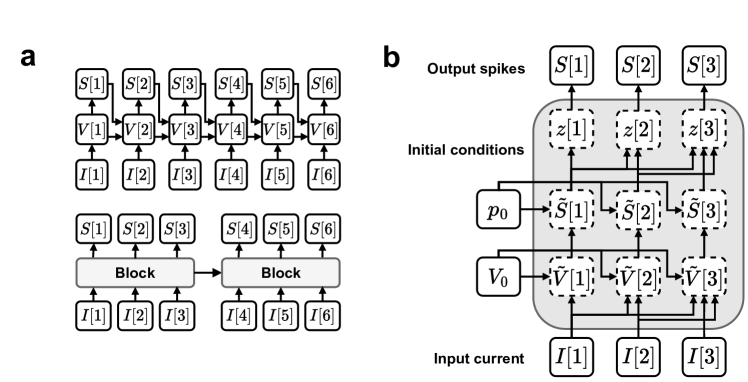
Figure 2: Solution overview. a. Our proposed solution: instead of simulating network dynamics one time step after another (top), we sequentially simulate blocks of time equal in length to the neuron ARP (bottom), in which a neuron can spike at most once. b. A schematic of a Block: our proposed solution for emulating ALIF dynamics with a constant sequential complexity $O(1)$ over a short duration in which a neuron spikes at most once.

We outline a novel reformulation of the ALIF model, which theoretically reduces the sequential simulation complexity from $O(T)$ to $O(T/T_{R})$ (for simulation length $T$ and ARP length $T_{R}$). Using the observation that a neuron can spike at most once over simulation length $T_{R}$ (equal to the ARP; Figure 1c), we propose simulating network dynamics sequentially in blocks of length $T_{R}$ - as opposed to simulating every time step individually (Figure 2a) - as we show that these blocks can be simulated with a constant sequential complexity $O(1)$. Our reformulated ALIF model is mathematically the same as the standard ALIF model, but substantially faster to simulate and train. All the proofs for the propositions can be found in the Supplementary material.

3.1 Block: simulating single-spike ALIF dynamics with a constant sequential complexity

A SNN exhibits a sequential dependence due to the spike reset mechanism, where a neuron’s membrane potential $V_{i}[t]$ can be reset based on its previous output $S_{i}[t-1]$. Consequently, the simulation of a SNN necessitates a sequential approach. This restriction can, however, be alleviated if we assume a neuron to spike at most once over a particular simulation length (such as the ARP). The following steps - grouped together into a module referred to as a Block (Figure 2b) - compute ALIF dynamics (assuming at most one spike) without any sequential operations.

$$\tilde{V}_{i}[t] =\big{(}I_{i}*\tilde{\beta}_{i}\big{)}[t]\quad\text{(No-reset membrane potential)}$$ (6)

$$\tilde{S}_{i}[t] =f(\tilde{V}_{i}[t])\quad\textrm{(Faulty output spikes)}$$ (7)

$$z_{i}[t] =\phi(\tilde{S}_{i})[t]\quad\textrm{(Latent timing of spikes)}$$ (8)

$$S_{i}[t] =\mathbb{1}_{\displaystyle z_{i}[t]=1}\quad\textrm{(Correct output spikes)}$$ (9)

1. Calculate membrane potentials without reset

The first step in the Block (Equation 6) converts input current $I_{i}[t]$ to membrane potentials $\tilde{V}_{i}[t]$ without spike reset (i.e. excluding the reset mechanism in Equation 2). This transformation is achieved using a convolution (Proposition 1), thus avoiding any sequential operations.

Proposition 1.

Membrane potentials without spike reset are computed as a convolution $\tilde{V}_{i}[t]=\big{(}I_{i}*\tilde{\beta}_{i}\big{)}[t]$ between input current $I_{i}[t]$ and kernel $\tilde{\beta}_{i}[t]=(1-\beta_{i})\beta_{i}^{t}$ with the initial membrane potential encoded as $I_{i}[0]=\frac{V_{i}[0]}{1-\beta_{i}}$.

2. Faulty output spikes

No-reset membrane potentials $\tilde{V}_{i}[t]$ are mapped to erroneous output spikes $\tilde{S}_{i}[t]=f(\tilde{V}_{i}[t])$ (Equation 7) using spike function $f$ (Equation 1). This output can contain more than one spike, but only the first spike complies with the standard model dynamics, due to the omission of the reset mechanism and ARP constraint. Thus, to ensure that the Block only emits a single spike, all spikes succeeding the first spike occurrence are removed using the following steps.

3. Latent timing of spikes

Erroneous spike output $\tilde{S}_{i}[t]$ is mapped to a latent representation $z_{i}[t]=\phi(\tilde{S}_{i})[t]$ (Equation 8), encoding the timing of spikes. Function $\phi(\cdot)$ (taking vector $\tilde{S}_{i}$ as input; Proposition 2) is constructed to map all erroneous spikes $\tilde{S}_{i}[t]$, besides the first spike occurrence, to a value other than one (i.e. $z_{i}[t]\neq 1$ for all $t$ except for the smallest $t$ satisfying $\tilde{S}_{i}[t]=1$ if such $t$ exists).

Proposition 2.

Function $\phi(\tilde{S}_{i})[t]=\sum_{k=1}^{t}\tilde{S}_{i}[k](t-k+1)$ acting on $\tilde{S}_{i}\in\{0,1\}^{T}$ contains at most one element equal to one $\phi(\tilde{S}_{i})[t]=1$ for the smallest $t$ satisfying $\tilde{S}_{i}[t]=1$ (if such $t$ exists).

4. Correct output spikes

Lastly, the correct spike output $S_{i}[t]=\mathbb{1}_{\displaystyle z_{i}[t]=1}$ is obtained by setting every value in $z_{i}[t]$, besides the value one (i.e. the first spike), to zero (Equation 9).

3.2 Blocks: simulating ALIF SNN dynamics with a $O(T/T_{R})$ sequential complexity

The standard ALIF SNN model can be reformulated using a chaining of Blocks, which reduces the sequential simulation complexity (as each Block is simulated in $O(1)$). For a given ARP of length $T_{R}$, we observed that a neuron spikes at most once over simulation length $T_{R}$ (Figure 1c). Thus, a simulation length $T$ can be simulated using $N=\frac{T}{T_{R}}$ Blocks, each of length $T_{R}$. Next, we outline how to simulate ALIF dynamics across Blocks to emulate the dynamics of the standard ALIF SNN. We introduce new notation to index Block $1\leq n\leq N$ using subscript $n$ (e.g. input current to neuron $i$ simulated in Block $n$ is expressed as $I_{i,n}[t]$) with time steps indexed between $[1,T_{R}]$ (as opposed to $[1,T]$) within a Block.

Input current and the ARP of a Block

The input current in the standard model (Equation 3 and 4) is modified for the Block model (Proposition 3). The feedforward and recurrent current to Block $n+1$ are derived from the presynaptic and postsynaptic spikes from Block $n+1$ and Block $n$ respectively. In addition, the ARP is enforced by applying a mask derived from the latent timing of spikes $z_{i,n}[t]$ (Equation 8).

Proposition 3.

The input current $I_{i,n+1}[t]$ of neuron $i$ simulated in Block $n+1$ (of length $T_{R}$) is defined as follows, and enforces an absolute refractory period of length $T_{R}$ and a monosynaptic transmission latency of $D=T_{R}$.

$$I_{i,n+1}[t]=\Big{(}b_{i}+\underbrace{\sum_{j=1}^{N^{\text{in}}}W_{ij}S_{j,n+1}[t]}_{\text{Feedforward current}}+\underbrace{\sum_{j=1}^{N^{\text{out}}}W^{\text{rec}}_{ij}S_{j,n}[t]}_{\text{Recurrent current}}\Big{)}\underbrace{\mathbb{1}_{\displaystyle z_{i,n}[t]\geq\max_{t}S_{i,n}[t]}\vphantom{\sum_{j=1}^{N^{(l)}}}}_{\text{ARP mask}}$$

Evolving membrane potentials between Blocks

Two cases are distinguished to correctly emulate the evolution of the membrane potentials between Blocks (Proposition 4): 1) if neuron $i$ did not spike in Block $n$ (i.e. $\max_{t}S_{i,n}[t]=0$), then its initial membrane potential $V_{i,n+1}[0]$ in Block $n+1$ is set to its final membrane potential $V_{i,n}[T_{R}]$ in Block $n$. Otherwise 2), the initial membrane potential is set to zero to emulate a spike reset (and no state needs to be transferred between Blocks as the neuron is in a refractory state).

Proposition 4.

The initial membrane potential $V_{i,n+1}[0]$ of neuron $i$ simulated in Block $n+1$ (of length $T_{R}$) is equal to the last membrane potential in Block $n$ if no spike occurred and zero otherwise.

$$V_{i,n+1}[0]=\begin{cases}V_{i,n}[T_{R}]&\text{if }\max_{t}S_{i,n}[t]=0\\ 0&\text{otherwise}\end{cases}$$

Evolving adaptive firing thresholds between Blocks

The adaptive firing threshold $\theta_{i,n+1}[t]$ of neuron $i$ in Block $n+1$ is derived from the initial adaptive parameter $a_{i,n+1}[0]$ (Proposition 5). Two cases are distinguished for deriving this parameter: 1) if the neuron did not spike during the previous Block $n$, this parameter is set to its last value, $a_{i,n}[T_{R}]$, in the prior Block; otherwise 2), the effect of the spike needs to be taken into account, for which the initial adaptive parameter is expressed as $p_{i}^{m}(a_{s}+p_{i}^{-1})$. Here, $m$ is the number of time steps remaining in Block $n$ following the spike and $a_{s}$ is the adaptive parameter value at the time of spiking.

Proposition 5.

The adaptive firing threshold $\theta_{i,n+1}[t]$ of neuron $i$ simulated in Block $n+1$ (of length $T_{R}$) is constructed from the initial adaptive parameter $a_{i,n+1}[0]$, which is equal to its last value in the previous Block if no spike occurred, and otherwise equal to an expression which accounts for the effect of the spike on the adaptive threshold.

$$\theta_{i,n+1}[t] =1+d_{i}p_{i}^{t}a_{i,n+1}[0]$$

$$a_{i,n+1}[0] =\begin{cases}a_{i,n}[T_{R}]&\text{if }\max_{t}{S_{i,n}[t]}=0\\ p_{i}^{m}(a_{s}+p_{i}^{-1})&\text{otherwise}\end{cases}$$

$$m=\sum_{k}^{T_{R}} \mathbb{1}_{\displaystyle z_{i,n}[k]>1},\quad a_{s}=\sum_{k}^{T_{R}}a_{i,n}[k]S_{i,n}[k]$$

3.3 Theoretical speedup for simulating ALIF SNNs using Blocks

Method	Computational Complexity	Sequential Operations
Standard	$O(N^{\text{in}}N^{\text{out}}T)$	$O(T)$
Blocks	$O(N^{\text{in}}N^{\text{out}}T_{R}^{2}N)$	$O(T/T_{R})$

Table 1: Computational and sequential complexity of simulating a layer of $N^{\text{out}}$ neurons with $N^{\text{in}}$ input neurons for $T$ time steps using the standard method and our method (with $N$ Blocks each of length $T_{R}$).

Simulating an ALIF SNN using our Blocks, rather than the conventional approach, requires fewer sequential operations (Table 1). Although the computational complexity of our Blocks approach is larger than the standard approach, the number of sequential operations is less. If we assume that the sequential steps in both methods are executed in an equal amount of time (as all the non-sequential operations can be run in parallel on a GPU), we obtain a theoretical speedup equal to the length of the ARP $\frac{T}{N}=T_{R}$.

4 Experiments

We evaluated the training speedup of our accelerated ALIF SNN relative to the standard ALIF SNN and explored the capacity of our model to be fitted using different spiking classification datasets and real electrophysiological recordings of cortical neurons. Implementation details can be found in the Supplementary material and the code at https://github.com/webstorms/Blocks.

4.1 Training speedup scales with an increasing ARP

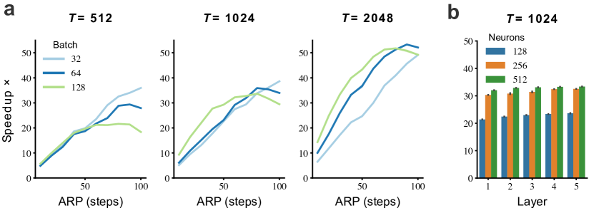
Figure 3: Training speedup of our model. a. Training speedup of our accelerated ALIF model compared to the standard ALIF model for different simulation lengths $T$, ARP time steps and batch sizes. b. Training speedup over different number of layers and hidden units (with an ARP of $T_{R}=40$ time steps, $T=1024$ time steps and batch size $=64$; bars plot the mean and standard error over ten runs). Assuming DT$=0.1$ms, then $10$ time steps $=1$ms.

To determine how much faster our model is, we benchmarked the required training duration (forward and backward pass) of our accelerated ALIF SNN to the standard ALIF SNN for varying ARP and simulation lengths using a synthetic spike dataset, with the task of minimizing the number of final-layer output spikes (see Supplementary material). We found the training speedup of our model to increase for a growing ARP (Figure 3a). This speedup was more pronounced for longer simulation durations ($53\times$ speedup for $T=2048$) than shorter simulation durations ($36\times$ speedup for $T=512$). These speedups were also present when just running the forward pass (i.e. inference using the network; see Supplementary material). Furthermore, we found the speedup of our model to be robust over varying numbers of neurons and layers (Figure 3b). Lastly, we also found our method to perform the forward pass more than an order of magnitude faster than other publicly available SNN implementations [63, 64] (see Supplementary material).

4.2 Accelerated training on spiking classification tasks

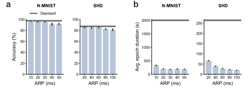
Figure 4: Performance of our model on spiking datasets. a. Classification accuracy of our model and the standard ALIF SNN on the N-MNIST and SHD datasets over different (non-biological) ARPs (N-MNIST $1$ms$=$1 time step; SHD $2$ms$=$1 time step). b. Training durations of our model and the standard ALIF SNN on the N-MNIST and SHD datasets. Horizontal gray lines plot the standard model’s performance (using no ARP) and bars plot the mean and standard error over three runs.

To establish whether our model can learn using backprop with surrogate gradients, and perform on a par with the standard model, we trained our accelerated ALIF SNN and the standard ALIF SNN on the Neuromophic-MNIST (N-MNIST) (using DT$=1$ms) [65] and Spiking Heidelberg Digits (SHD) (using DT$=2$ms) [66] spiking classification datasets (both commonly used for benchmarking SNN performance [40, 67, 29, 42, 50]). The task of the N-MNIST dataset is to classify spike representations of handwritten digits, and the task of the SHD dataset is to classify spike representations of spoken digits. In all experiments we employed identical model architectures consisting of two hidden layers (of $256$ neurons each) and an additional integrator readout layer, with predictions taken from the readout neurons with maximal summated membrane potential over time (as commonly done [66, 68, 29, 42, 50]; see Supplementary material). We adopted the multi-Gaussian surrogate-gradient function [29] to overcome the non-differentiable discontinuity of the spike function (although we found that other surrogate-gradient functions also work, see Supplementary material). Furthermore (as suggested by [68] for conventional SNNs), we only permitted surrogate gradients to flow through the non-recurrent connectivity (which significantly improved performance; see Supplementary material).

We trained our model with different non-biological ARPs on each dataset and contrasted the accuracy and training duration to the standard model (with no ARP). We found a favourable trade-off between classification accuracy and training time for our model. Compared to the standard ALIF SNN model, our model achieved a very similar, albeit slightly lower, accuracy on the N-MNIST ($96.97\%$ for ARP=$10$ms vs standard $97.71\%$) and SHD dataset ($86.07\%$ for ARP=$20$ms vs standard $87.48\%$), with the accuracy declining only for the largest ARPs tested (Figure 4a). However, our model only required a fraction of the training time, with an average training epoch of $181$s and $20$s for the N-MNIST and SHD datasets, respectively, when using the largest tested ARP, compared to the respective standard model training times of $2034$s and $268$s (Figure 4b).

4.3 Quickly fitting real neural recordings on sub-millisecond timescales

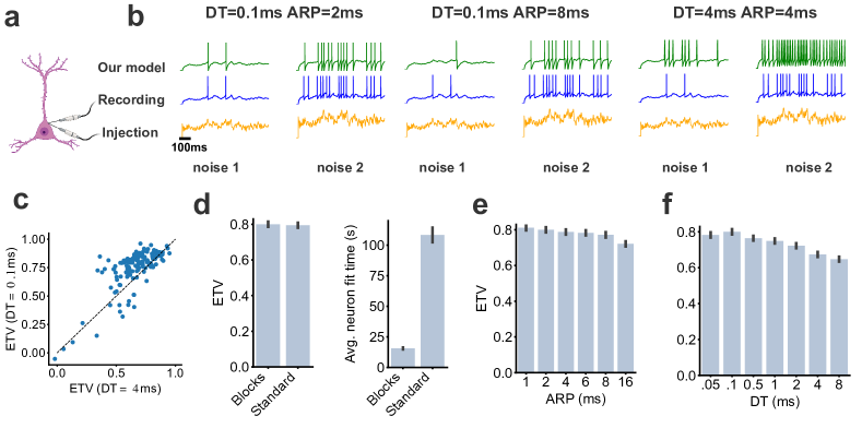
Figure 5: Fitting cortical electrophysiological recordings. a. An illustration of a cortical neuron in mouse V1 being recorded whilst stimulated with a noisy current injection. b. For held-out data not used for fitting, an example current injection (bottom) and recorded membrane potential (middle) with corresponding fitted model predictions (top). c. Comparison of neuron fit accuracy of our model for DT$=0.1$ms (y-axis) against DT$=4$ms (x-axis). Explained temporal variance (ETV) measures the goodness-of-fit (one is a perfect fit and zero is a chance-level fit). d. Comparison of the fit accuracy (left) and duration (right) of our model and the standard model (both using DT$=0.1$ms and ARP$=2$ms). e. Our model’s fit accuracy for increasing ARP (with DT$=0.1$ms). f. Our model’s fit accuracy for increasing DT (with ARP=$\text{max}(2,\text{DT})$ms). d. to f. plots the median and standard error over neurons, except that d. (right) plots the mean fit time.

We explored the ability of our model to fit in vitro electrophysiological recordings from $146$ inhibitory and excitatory neurons in mouse primary visual cortex (V1) (provided by the Allen Institute [69, 70]). In these recordings, a variable input current was repeatedly injected at various amplitudes into each real neuron, and the resulting alteration in the membrane potential was recorded (Figure 5a). For each neuron, we used half of the recordings for fitting and the other half for testing, and report all the qualitative and quantitative results on the held-out test dataset. Fitting was achieved by minimising the van Rossum distance between the model and real spike trains [71]. To quantitatively compare the fits of our model using different DTs and ARPs, we employed the explained temporal variance (ETV) measure (used on the Allen Institute website; see Supplementary material). This metric quantifies how well the temporal dynamics of the neurons are captured by the model and takes into account trial-to-trial variability due to intrinsic neural noise. It has a value of one for a perfect fit and a value of zero if the model predicts at chance.

We found that our accelerated ALIF model captured the spike timing of the neurons. Pertinent to the speed-accuracy trade-off, this fit strongly depended on the chosen DT, and less so on the chosen ARP. Qualitatively, using a DT$=0.1$ms and an ARP$=2$ms, we found our model captured the spike timings of the neurons for current injections of varying amplitude. This still seemed to be the case when we used a larger ARP$=8$ms, but the model was worse at capturing spike timings when we used a larger DT$=4$ms (with ARP$=4$ms; Figure 5b; see Supplementary material for zoomed-in neural traces).

Quantitatively comparing the neuron fits one by one, we found that nearly all of the neuron fits were better when using a DT$=0.1$ms (ETV$=0.80$) than a DT$=4$ms (ETV$=0.66$; Figure 5c; using an ARP$=4$ms). We examined how accurate and fast our fits were compared to the standard model using an ARP$=2$ms and a DT$=0.1$ms. Both models achieved a similar ETV of $\sim 0.8$, yet our model only required $15.5$s on average per neuron fit time compared to the $108.4$s of the standard model (Figure 5d). We further investigated whether a larger ARP could still reasonably fit the data for DT$=0.1$ms (to benefit from a faster fit). Consistent with our qualitative observations, we found a less marked reduction in fit accuracy when using larger ARPs (Figure 5e) compared to the drop in performance when using larger DTs (Figure 5f; using an ARP of $\text{max}(2,\text{DT})$ms).

5 Discussion

ALIF neurons are a popular model for studying the brain in silico. Training these neurons is, however, slow due to their sequential nature [41, 72]. We overcome this by algorithmically reinterpreting the ALIF model. We found that our method permits faster simulation of SNNs, which will likely play an important role in future research into neural dynamics through simulation [17, 16]. We also confirmed the validity of this approach for modelling neural data. Firstly - of interest to computational neuroscientists - we fitted a multilayered network of neurons using two common spike classification datasets. We found that our model achieved a similar classification accuracy to that of the standard model, even if we increased the ARP to large non-physiological values, which drastically reduced the training duration required for both datasets. Secondly - of interest to computational and experimental neuroscientists - we explored the applicability of our method to fit real electrophysiological recordings of neurons in mouse V1 using sub-millisecond DTs.

We found that our method accurately captured the spike timing of real neurons, fitting their activity patterns in a fraction of the time required by the standard model (although we note that other, more recent spiking-models, might improve fit accuracies [73]). This is particularly important as datasets become larger with advances in recording techniques, requiring faster fitting solutions to characterise computational properties of neurons. As an example of the potential insights provided by our model, we found the fitted V1 neurons to have a heterogenous membrane time constant distribution, suggesting that V1 processes visual information on multiple timescales [42] (see Supplementary material).

Our work will likely also be of interest to neuromorphic engineers and researchers, developing energy-efficient hardware to emulate SNNs [20]. These systems - like real neurons - run in continuous time and thus require training on extremely fine DTs off-chip [74, 75]. Our method could help to accelerate off-chip training times. Furthermore, the ARP hyperparameter in our model can limit high spike rates and thus reduce energy consumption on neuromorphic systems, as this consumption scales approximately proportionally with the number of emitted spikes [76].

A limitation of our method is that the training speedup scales sublinearly - as opposed to linearly - with an increasing ARP simulation length (see Section 3 and 4.1). This is likely due to GPU overheads and employed cudnn routines [77], which further improvements to our code implementation could overcome. An additional limitation is the requirement to define the ARP hyperparameter, whose value influences the training speed and test accuracy in our method and relates to biological realism. However, we found a beneficial trade-off - by using large non-biological ARPs on the artificial spiking classification dataset and small physiological ARPs for the neural fits (although we found larger values to also perform reasonably well) the model achieved comparable accuracy to the standard ALIF model in both cases, while also having greatly increased speed of training and simulation. In particular, the capacity of our model to accurately and quickly fit the data from real neurons is crucial in terms of the biological applicability of this approach.

References

- Harper et al. [2016] Nicol S Harper, Oliver Schoppe, Ben DB Willmore, Zhanfeng Cui, Jan WH Schnupp, and Andrew J King. Network receptive field modeling reveals extensive integration and multi-feature selectivity in auditory cortical neurons. PLoS Computational Biology, 12(11):e1005113, 2016.
- Singer et al. [2023] Yosef Singer, Luke Taylor, Ben DB Willmore, Andrew J King, and Nicol S Harper. Hierarchical temporal prediction captures motion processing along the visual pathway. eLife, 12:e52599, 2023.
- Cadena et al. [2019] Santiago A Cadena, George H Denfield, Edgar Y Walker, Leon A Gatys, Andreas S Tolias, Matthias Bethge, and Alexander S Ecker. Deep convolutional models improve predictions of macaque v1 responses to natural images. PLoS Computational Biology, 15(4):e1006897, 2019.
- Francl and McDermott [2022] Andrew Francl and Josh H McDermott. Deep neural network models of sound localization reveal how perception is adapted to real-world environments. Nature Human Behaviour, 6(1):111–133, 2022.
- Yamins and DiCarlo [2016] Daniel LK Yamins and James J DiCarlo. Using goal-driven deep learning models to understand sensory cortex. Nature Neuroscience, 19(3):356–365, 2016.
- Bakhtiari et al. [2021] Shahab Bakhtiari, Patrick Mineault, Timothy Lillicrap, Christopher Pack, and Blake Richards. The functional specialization of visual cortex emerges from training parallel pathways with self-supervised predictive learning. Advances in Neural Information Processing Systems, 34:25164–25178, 2021.
- Mineault et al. [2021] Patrick Mineault, Shahab Bakhtiari, Blake Richards, and Christopher Pack. Your head is there to move you around: Goal-driven models of the primate dorsal pathway. Advances in Neural Information Processing Systems, 34:28757–28771, 2021.
- Ocko et al. [2018] Samuel Ocko, Jack Lindsey, Surya Ganguli, and Stephane Deny. The emergence of multiple retinal cell types through efficient coding of natural movies. Advances in Neural Information Processing Systems, 31, 2018.
- Conwell et al. [2021] Colin Conwell, David Mayo, Andrei Barbu, Michael Buice, George Alvarez, and Boris Katz. Neural regression, representational similarity, model zoology & neural taskonomy at scale in rodent visual cortex. Advances in Neural Information Processing Systems, 34:5590–5607, 2021.
- Richards et al. [2019] Blake A Richards, Timothy P Lillicrap, Philippe Beaudoin, Yoshua Bengio, Rafal Bogacz, Amelia Christensen, Claudia Clopath, Rui Ponte Costa, Archy de Berker, Surya Ganguli, et al. A deep learning framework for neuroscience. Nature Neuroscience, 22(11):1761–1770, 2019.
- Jolivet et al. [2008] Renaud Jolivet, Felix Schürmann, Thomas K Berger, Richard Naud, Wulfram Gerstner, and Arnd Roth. The quantitative single-neuron modeling competition. Biological Cybernetics, 99:417–426, 2008.
- Kobayashi et al. [2009] Ryota Kobayashi, Yasuhiro Tsubo, and Shigeru Shinomoto. Made-to-order spiking neuron model equipped with a multi-timescale adaptive threshold. Frontiers in Computational Neuroscience, page 9, 2009.
- Rossant et al. [2011] Cyrille Rossant, Dan FM Goodman, Bertrand Fontaine, Jonathan Platkiewicz, Anna K Magnusson, and Romain Brette. Fitting neuron models to spike trains. Frontiers in Neuroscience, 5:9, 2011.
- Mensi et al. [2012] Skander Mensi, Richard Naud, Christian Pozzorini, Michael Avermann, Carl CH Petersen, and Wulfram Gerstner. Parameter extraction and classification of three cortical neuron types reveals two distinct adaptation mechanisms. Journal of Neurophysiology, 107(6):1756–1775, 2012.
- Pozzorini et al. [2013] Christian Pozzorini, Richard Naud, Skander Mensi, and Wulfram Gerstner. Temporal whitening by power-law adaptation in neocortical neurons. Nature Neuroscience, 16(7):942–948, 2013.
- Denève and Machens [2016] Sophie Denève and Christian K Machens. Efficient codes and balanced networks. Nature Neuroscience, 19(3):375–382, 2016.
- Vogels et al. [2011] Tim P Vogels, Henning Sprekeler, Friedemann Zenke, Claudia Clopath, and Wulfram Gerstner. Inhibitory plasticity balances excitation and inhibition in sensory pathways and memory networks. Science, 334(6062):1569–1573, 2011.
- Confavreux et al. [2020] Basile Confavreux, Friedemann Zenke, Everton Agnes, Timothy Lillicrap, and Tim Vogels. A meta-learning approach to (re) discover plasticity rules that carve a desired function into a neural network. Advances in Neural Information Processing Systems, 33:16398–16408, 2020.
- Braun and Vogels [2021] Lukas Braun and Tim Vogels. Online learning of neural computations from sparse temporal feedback. Advances in Neural Information Processing Systems, 34:16437–16450, 2021.
- Wunderlich et al. [2019] Timo Wunderlich, Akos F Kungl, Eric Müller, Andreas Hartel, Yannik Stradmann, Syed Ahmed Aamir, Andreas Grübl, Arthur Heimbrecht, Korbinian Schreiber, David Stöckel, et al. Demonstrating advantages of neuromorphic computation: a pilot study. Frontiers in Neuroscience, 13:260, 2019.
- Lapicque [1907] Louis Lapicque. Recherches quantitatives sur l’excitation electrique des nerfs traitee comme une polarization. Journal de physiologie et de pathologie générale, 9:620–635, 1907.
- Gerstner et al. [2014] Wulfram Gerstner, Werner M Kistler, Richard Naud, and Liam Paninski. Neuronal dynamics: From single neurons to networks and models of cognition. Cambridge University Press, 2014.
- Kandel et al. [2000] Eric R Kandel, James H Schwartz, Thomas M Jessell, Steven Siegelbaum, A James Hudspeth, Sarah Mack, et al. Principles of neural science, Fourth edition. Elsevier, 2000.
- Levakova et al. [2019] Marie Levakova, Lubomir Kostal, Christelle Monsempès, Philippe Lucas, and Ryota Kobayashi. Adaptive integrate-and-fire model reproduces the dynamics of olfactory receptor neuron responses in a moth. Journal of the Royal Society Interface, 16(157):20190246, 2019.
- Zeng et al. [2021] Yuan Zeng, Terrence C Stewart, Zubayer Ibne Ferdous, Yevgeny Berdichevsky, and Xiaochen Guo. Temporal learning with biologically fitted snn models. In International Conference on Neuromorphic Systems 2021, pages 1–8, 2021.
- Bellec et al. [2018] Guillaume Bellec, Darjan Salaj, Anand Subramoney, Robert Legenstein, and Wolfgang Maass. Long short-term memory and learning-to-learn in networks of spiking neurons. Advances in neural information processing systems, 31, 2018.
- Bellec et al. [2020] Guillaume Bellec, Franz Scherr, Anand Subramoney, Elias Hajek, Darjan Salaj, Robert Legenstein, and Wolfgang Maass. A solution to the learning dilemma for recurrent networks of spiking neurons. Nature Communications, 11(1):1–15, 2020.
- Yin et al. [2020] Bojian Yin, Federico Corradi, and Sander M Bohté. Effective and efficient computation with multiple-timescale spiking recurrent neural networks. In International Conference on Neuromorphic Systems 2020, pages 1–8, 2020.
- Yin et al. [2023] Bojian Yin, Federico Corradi, and Sander M Bohté. Accurate online training of dynamical spiking neural networks through forward propagation through time. Nature Machine Intelligence, pages 1–10, 2023.
- Perez-Nieves and Goodman [2023] Nicolas Perez-Nieves and Dan FM Goodman. Spiking network initialisation and firing rate collapse. arXiv:2305.08879, 2023.
- Yin et al. [2021] Bojian Yin, Federico Corradi, and Sander M Bohté. Accurate and efficient time-domain classification with adaptive spiking recurrent neural networks. Nature Machine Intelligence, 3(10):905–913, 2021.
- Andersen et al. [1978] P Andersen, H Silfvenius, SH Sundberg, On Sveen, H Wigstro, et al. Functional characteristics of unmyelinated fibres in the hippocampal cortex. Brain research, 144(1):11–18, 1978.
- Avissar et al. [2013] Michael Avissar, John H Wittig, James C Saunders, and Thomas D Parsons. Refractoriness enhances temporal coding by auditory nerve fibers. Journal of Neuroscience, 33(18):7681–7690, 2013.
- Rolls [1971] Edmund T Rolls. Absolute refractory period of neurons involved in mfb self-stimulation. Physiology & Behavior, 7(3):311–315, 1971.
- Jouhanneau et al. [2015] Jean-Sébastien Jouhanneau, Jens Kremkow, Anja L Dorrn, and James FA Poulet. In vivo monosynaptic excitatory transmission between layer 2 cortical pyramidal neurons. Cell reports, 13(10):2098–2106, 2015.
- Rumelhart et al. [1986] David E Rumelhart, Geoffrey E Hinton, and Ronald J Williams. Learning representations by back-propagating errors. Nature, 323(6088):533–536, 1986.
- Esser et al. [2016] Steven K Esser, Paul A Merolla, John V Arthur, Andrew S Cassidy, Rathinakumar Appuswamy, Alexander Andreopoulos, David J Berg, Jeffrey L McKinstry, Timothy Melano, Davis R Barch, et al. Convolutional networks for fast, energy-efficient neuromorphic computing. Proceedings of the National Academy of Sciences, 113(41):11441–11446, 2016.
- Hunsberger and Eliasmith [2015] Eric Hunsberger and Chris Eliasmith. Spiking deep networks with lif neurons. arXiv:1510.08829, 2015.
- Zenke and Ganguli [2018] Friedemann Zenke and Surya Ganguli. Superspike: Supervised learning in multilayer spiking neural networks. Neural Computation, 30(6):1514–1541, 2018.
- Lee et al. [2016] Jun Haeng Lee, Tobi Delbruck, and Michael Pfeiffer. Training deep spiking neural networks using backpropagation. Frontiers in Neuroscience, 10:508, 2016.
- Neftci et al. [2019] Emre O Neftci, Hesham Mostafa, and Friedemann Zenke. Surrogate gradient learning in spiking neural networks: Bringing the power of gradient-based optimization to spiking neural networks. IEEE Signal Processing Magazine, 36(6):51–63, 2019.
- Perez-Nieves et al. [2021] Nicolas Perez-Nieves, Vincent CH Leung, Pier Luigi Dragotti, and Dan FM Goodman. Neural heterogeneity promotes robust learning. Nature communications, 12(1):1–9, 2021.
- O’Connor et al. [2013] Peter O’Connor, Daniel Neil, Shih-Chii Liu, Tobi Delbruck, and Michael Pfeiffer. Real-time classification and sensor fusion with a spiking deep belief network. Frontiers in Neuroscience, 7:178, 2013.
- Esser et al. [2015] Steve K Esser, Rathinakumar Appuswamy, Paul Merolla, John V Arthur, and Dharmendra S Modha. Backpropagation for energy-efficient neuromorphic computing. Advances in neural information processing systems, 28, 2015.
- Rueckauer et al. [2016] Bodo Rueckauer, Iulia-Alexandra Lungu, Yuhuang Hu, and Michael Pfeiffer. Theory and tools for the conversion of analog to spiking convolutional neural networks. arXiv:1612.04052, 2016.
- Rueckauer et al. [2017] Bodo Rueckauer, Iulia-Alexandra Lungu, Yuhuang Hu, Michael Pfeiffer, and Shih-Chii Liu. Conversion of continuous-valued deep networks to efficient event-driven networks for image classification. Frontiers in Neuroscience, 11:682, 2017.
- Gewaltig and Diesmann [2007] Marc-Oliver Gewaltig and Markus Diesmann. Nest (neural simulation tool). Scholarpedia, 2(4):1430, 2007.
- Morrison et al. [2005] Abigail Morrison, Carsten Mehring, Theo Geisel, AD Aertsen, and Markus Diesmann. Advancing the boundaries of high-connectivity network simulation with distributed computing. Neural computation, 17(8):1776–1801, 2005.
- Morrison et al. [2007] Abigail Morrison, Sirko Straube, Hans Ekkehard Plesser, and Markus Diesmann. Exact subthreshold integration with continuous spike times in discrete-time neural network simulations. Neural Computation, 19(1):47–79, 2007.
- Perez-Nieves and Goodman [2021] Nicolas Perez-Nieves and Dan Goodman. Sparse spiking gradient descent. Advances in Neural Information Processing Systems, 34:11795–11808, 2021.
- Williams and Zipser [1989] Ronald J Williams and David Zipser. A learning algorithm for continually running fully recurrent neural networks. Neural Computation, 1(2):270–280, 1989.
- Kag and Saligrama [2021] Anil Kag and Venkatesh Saligrama. Training recurrent neural networks via forward propagation through time. In International Conference on Machine Learning, pages 5189–5200. PMLR, 2021.
- Murray [2019] James M Murray. Local online learning in recurrent networks with random feedback. Elife, 8:e43299, 2019.
- Bohte et al. [2002] Sander M Bohte, Joost N Kok, and Han La Poutre. Error-backpropagation in temporally encoded networks of spiking neurons. Neurocomputing, 48(1-4):17–37, 2002.
- Mostafa [2017] Hesham Mostafa. Supervised learning based on temporal coding in spiking neural networks. IEEE transactions on neural networks and learning systems, 29(7):3227–3235, 2017.
- Comsa et al. [2020] Iulia M Comsa, Krzysztof Potempa, Luca Versari, Thomas Fischbacher, Andrea Gesmundo, and Jyrki Alakuijala. Temporal coding in spiking neural networks with alpha synaptic function. In ICASSP 2020-2020 IEEE International Conference on Acoustics, Speech and Signal Processing (ICASSP), pages 8529–8533. IEEE, 2020.
- Kheradpisheh and Masquelier [2020] Saeed Reza Kheradpisheh and Timothée Masquelier. Temporal backpropagation for spiking neural networks with one spike per neuron. International Journal of Neural Systems, 30(06):2050027, 2020.
- Zhang et al. [2021] Malu Zhang, Jiadong Wang, Jibin Wu, Ammar Belatreche, Burin Amornpaisannon, Zhixuan Zhang, Venkata Pavan Kumar Miriyala, Hong Qu, Yansong Chua, Trevor E Carlson, et al. Rectified linear postsynaptic potential function for backpropagation in deep spiking neural networks. IEEE Transactions on Neural Networks and Learning Systems, 33(5):1947–1958, 2021.
- Zhou and Li [2021] Shibo Zhou and Xiaohua Li. Spiking neural networks with single-spike temporal-coded neurons for network intrusion detection. In 2020 25th International Conference on Pattern Recognition (ICPR), pages 8148–8155. IEEE, 2021.
- Zhou et al. [2021] Shibo Zhou, Xiaohua Li, Ying Chen, Sanjeev T Chandrasekaran, and Arindam Sanyal. Temporal-coded deep spiking neural network with easy training and robust performance. In Proceedings of the AAAI Conference on Artificial Intelligence, volume 35, pages 11143–11151, 2021.
- Göltz et al. [2021] Julian Göltz, Laura Kriener, Andreas Baumbach, Sebastian Billaudelle, Oliver Breitwieser, Benjamin Cramer, Dominik Dold, Akos Ferenc Kungl, Walter Senn, Johannes Schemmel, et al. Fast and energy-efficient neuromorphic deep learning with first-spike times. Nature Machine Intelligence, 3(9):823–835, 2021.
- Zhu et al. [2022] Yaoyu Zhu, Zhaofei Yu, Wei Fang, Xiaodong Xie, Tiejun Huang, and Timothée Masquelier. Training spiking neural networks with event-driven backpropagation. In 36th Conference on Neural Information Processing Systems (NeurIPS 2022), 2022.
- Pehle and Pedersen [2021] Christian Pehle and Jens Egholm Pedersen. Norse - A deep learning library for spiking neural networks, January 2021. URL https://doi.org/10.5281/zenodo.4422025. Documentation: https://norse.ai/docs/.
- Fang et al. [2023] Wei Fang, Yanqi Chen, Jianhao Ding, Zhaofei Yu, Timothée Masquelier, Ding Chen, Liwei Huang, Huihui Zhou, Guoqi Li, and Yonghong Tian. Spikingjelly: An open-source machine learning infrastructure platform for spike-based intelligence. Science Advances, 9(40):eadi1480, 2023.
- Orchard et al. [2015] Garrick Orchard, Ajinkya Jayawant, Gregory K Cohen, and Nitish Thakor. Converting static image datasets to spiking neuromorphic datasets using saccades. Frontiers in Neuroscience, 9:437, 2015.
- Cramer et al. [2020] Benjamin Cramer, Yannik Stradmann, Johannes Schemmel, and Friedemann Zenke. The heidelberg spiking data sets for the systematic evaluation of spiking neural networks. IEEE Transactions on Neural Networks and Learning Systems, 2020.
- Shrestha and Orchard [2018] Sumit B Shrestha and Garrick Orchard. Slayer: Spike layer error reassignment in time. Advances in neural information processing systems, 31, 2018.
- Zenke and Vogels [2021] Friedemann Zenke and Tim P Vogels. The remarkable robustness of surrogate gradient learning for instilling complex function in spiking neural networks. Neural Computation, 33(4):899–925, 2021.
- Lein et al. [2007] Ed S Lein, Michael J Hawrylycz, Nancy Ao, Mikael Ayres, Amy Bensinger, Amy Bernard, Andrew F Boe, Mark S Boguski, Kevin S Brockway, Emi J Byrnes, et al. Genome-wide atlas of gene expression in the adult mouse brain. Nature, 445(7124):168–176, 2007.
- Hawrylycz et al. [2012] Michael J Hawrylycz, Ed S Lein, Angela L Guillozet-Bongaarts, Elaine H Shen, Lydia Ng, Jeremy A Miller, Louie N Van De Lagemaat, Kimberly A Smith, Amanda Ebbert, Zackery L Riley, et al. An anatomically comprehensive atlas of the adult human brain transcriptome. Nature, 489(7416):391–399, 2012.
- van Rossum [2001] Mark CW van Rossum. A novel spike distance. Neural Computation, 13(4):751–763, 2001.
- Eshraghian et al. [2023] Jason K Eshraghian, Max Ward, Emre O Neftci, Xinxin Wang, Gregor Lenz, Girish Dwivedi, Mohammed Bennamoun, Doo Seok Jeong, and Wei D Lu. Training spiking neural networks using lessons from deep learning. Proceedings of the IEEE, 2023.
- Pozzorini et al. [2015] Christian Pozzorini, Skander Mensi, Olivier Hagens, Richard Naud, Christof Koch, and Wulfram Gerstner. Automated high-throughput characterization of single neurons by means of simplified spiking models. PLoS Computational Biology, 11(6):e1004275, 2015.
- Stuijt et al. [2021] Jan Stuijt, Manolis Sifalakis, Amirreza Yousefzadeh, and Federico Corradi. brain: An event-driven and fully synthesizable architecture for spiking neural networks. Frontiers in Neuroscience, page 538, 2021.
- He et al. [2021] Yuming He, Federico Corradi, Chengyao Shi, Ming Ding, Martijn Timmermans, Jan Stuijt, Pieter Harpe, Ilja Ocket, and Yao-Hong Liu. A 28.2 c neuromorphic sensing system featuring snn-based near-sensor computation and event-driven body-channel communication for insertable cardiac monitoring. In 2021 IEEE Asian Solid-State Circuits Conference (A-SSCC), pages 1–3. IEEE, 2021.
- Panda et al. [2020] Priyadarshini Panda, Sai Aparna Aketi, and Kaushik Roy. Toward scalable, efficient, and accurate deep spiking neural networks with backward residual connections, stochastic softmax, and hybridization. Frontiers in Neuroscience, 14:653, 2020.
- Chetlur et al. [2014] Sharan Chetlur, Cliff Woolley, Philippe Vandermersch, Jonathan Cohen, John Tran, Bryan Catanzaro, and Evan Shelhamer. cudnn: Efficient primitives for deep learning. arXiv:1410.0759, 2014.