Algorithms for Gromov-Witten Invariants of Elliptic Curves

Abstract.

We present an enhanced algorithm for exploring mirror symmetry for elliptic curves through the correspondence of algebraic and tropical geometry, focusing on Gromov-Witten invariants of elliptic curves and, in particular, Hurwitz numbers. We present a new highly efficient algorithm for computing generating series for these numbers. We have implemented the algorithm both using Singular and OSCAR. The implementations outperform by far the current method provided in Singular. The OSCAR implementation, benefiting in particular from just-in-time compilation, again by far outperforms the implementation of the new algorithm in Singular. This advancement in computing the Gromov-Witten invariants facilitates a study of number theoretic and geometric properties of the generating series, including quasi-modularity and homogeneity.

1. Introduction

Mirror symmetry is a deep duality relation motivated from physics. It relates invariants of a manifold and its ”mirror manifold” in a way allowing an exchange of methods. Tropical methods find a way into mirror symmetry most prominently in the famous Gross-Siebert programm [13].

Here, we present the special case of elliptic curves, for which mirror symmetry is best understood [12]. The tropical side of mirror symmetry for elliptic curves was discovered within the Collaborative Research Center SFB-TRR 195 [5, 7, 8], which is also responsible for the development of OSCAR.

One consequence of mirror symmetry for elliptic curves is the equality of the generating function of Hurwitz numbers (resp. more generally, of descendant Gromov-Witten invariants) to certain Feynman integrals which are complex analytic path integrals whose construction is governed by combinatorics.

Hurwitz numbers are traditional enumerative invariants that count covers of Riemann surfaces satisfying fixed ramification data. Their definition goes back to Hurwitz himself and was used to study the irreducibility of the famous moduli space of smooth genus $g$ curves, a fundamental object in algebraic geometry. In modern mathematics, Hurwitz numbers provide fruitful interactions between several mathematical areas such as geometry, topology, representation theory, combinatorics and mathematical physics [11].

Tropical geometry can be viewed as a degenerate version of algebraic geometry which has been used successfully to solve enumerative problems in algebraic geometry [16]. In particular, by counting tropical covers (see Definition 2.5), we can determine Hurwitz numbers via a so-called correspondence theorem [9, 5]. It allow to translate any computation we perform involving tropical covers to traditional Hurwitz theory.

In this chapter, we describe how one can use tropical mirror symmetry for elliptic curves in order to compute generating series for tropical Hurwitz numbers of an elliptic curve and their generalizations (up to fixed order) by means of computing Feynman integrals. We discuss explicit algorithms and implementations to handle this task. In [5] an algorithm to compute Hurwitz numbers via Feynman integrals has been described which works through computing coefficients in the Laurent series expansion of the propagator of the Feynman integral in terms of the integration variables. Based on this algorithm, we develop in this chapter a significantly improved version which shows a better performance when applied to current research problems. This algorithm works by assigning to each cover a so-called flip signature by considering the permutation assigning vertices of the source tropical curve to branch points on the target elliptic curve, observing that covers with the same signature lead to the same integral. Further improvements are achieved by direct computation of coefficients of the Laurent series, avoiding explicit expansion altogether. We have created two structurally identical implementations of the algorithm, one using the computer algebra system Singular and one using OSCAR. Both implementations outperform the previous algorithm of [5] in its implementation in Singular by far, which demonstrates the significant structural improvement in the algorithm. The OSCAR implementation again by far outperforms the implementation of the new algorithm in Singular. We attribute this to the just-in-time (JIT) compilation features, which turns at run-time easy-to-comprehend Julia code into code which executes almost as fast machine code, but also to superior arithmetic in OSCAR. This demonstrates the potential of the OSCAR platform.

2. Mirror Symmetry for Elliptic Curves

2.1. Hurwitz Numbers

Hurwitz numbers count branched covers of non-singular curves with a given ramification profile over fixed points. Here, we consider covers of elliptic curves. Hurwitz numbers are topological invariants, in particular they do not depend on the position of the branch points. Moreover, since all complex elliptic curves are homeomorphic to the real torus, numbers of covers of an elliptic curve do not depend on the choice of the base curve. We thus fix an arbitrary complex elliptic curve ${\mathcal{E}}$.

Let $\mathcal{C}$ be a non-singular curve of genus $g$ and $\phi:\mathcal{C}\rightarrow{\mathcal{E}}$ a cover. We denote by $d$ the degree of $\phi$, i.e., the number of preimages of a generic point in ${\mathcal{E}}$. For our purpose, it is sufficient to consider covers which are simply ramified, that is, over any branch point exactly two sheets of the map come together and all others stay separate. In other words, the ramification profile (that is, the partition of the degree indicating the multiplicities of the inverse images of a branch point) of a simple branch point is $(2,1,\ldots,1)$. It follows from the Riemann-Hurwitz formula (see e.g. [14], Corollary IV.2.4) that a simply ramified cover of ${\mathcal{E}}$ has exactly $2g-2$ branch points. Two covers $\varphi:\mathcal{C}\rightarrow{\mathcal{E}}$ and $\varphi^{\prime}:\mathcal{C}^{\prime}\rightarrow{\mathcal{E}}$ are isomorphic if there exists an isomorphism of curves $\phi:\mathcal{C}\rightarrow\mathcal{C}^{\prime}$ such that $\varphi^{\prime}\circ\phi=\varphi$.

Definition 2.1 (Hurwitz numbers).

Fix $2g-2$ points $p_{1},\ldots,p_{2g-2}$ in ${\mathcal{E}}$. We define the Hurwitz number $N_{d,g}$ to be the weighted number of (isomorphism classes of) simply ramified covers $\phi:\mathcal{C}\rightarrow{\mathcal{E}}$ of degree $d$, where $\mathcal{C}$ is a connected curve of genus $g$, and the branch points of $\phi$ are the points $p_{i}$, $i=1,\ldots,2g-2$. We count each such cover $\phi$ with weight $|\operatorname{Aut}(\phi)|$.

Remark 2.2.

Note that by convention, we fix a marking of the branch points $p_{i}$ in this definition. In the literature, one can also find definitions which do not follow this convention and do not mark the branch points, leading to a factor of $(2g-2)!$ when compared to our definition.

Definition 2.3.

We package the Hurwitz numbers of Definition 2.1 into a generating series as follows:

$$F_{g}(q):=\sum_{d=1}^{\infty}N_{d,g}q^{2d}.$$

2.2. Tropical Hurwitz Numbers

Definition 2.4 (Tropical curves).

A (generic) tropical curve $C$ (without ends) is a connected, finite, trivalent, metric graph. Its genus is given by its first Betti number. The combinatorial type of a curve is its homeomorphism class, that is, the underlying graph without lengths on the edges.

A tropical elliptic curve consists of one edge forming a circle of certain length. We will fix a tropical elliptic curve $E$ (for example, one having length $1$). Moreover, to fix notation, in the following we denote by $C$ a tropical curve of genus $g$ and combinatorial type $\Gamma$.

Definition 2.5 (Tropical covers).

A map $\pi:C\rightarrow E$ is a tropical cover of $E$ if it is continuous, non-constant, integer affine on each edge and respects the balancing condition at every vertex $P\in C$:

For an edge $e$ of $C$ denote by $w_{e}$ the weight of $e$, that is, the absolute value of the slope of $\pi_{|e}$. Consider a (small) open neighbourhood $U$ of $p=\pi(P)$. Then $U$ combinatorially consists of $p$ together with two rays $r_{1}$ and $r_{2}$, left and right of $p$. Let $V$ be the connected component of $\pi^{-1}(U)$ which contains $P$. Then $V$ consists of $P$ adjacent to three rays. Then $\pi$ is balanced at $P$ if

$$\sum_{R\mbox{{ \small maps to }}r_{1}}w_{R}=\sum_{R\mbox{ {\small maps to }}r_{2}}w_{R},$$

where $R$ goes over the three rays adjacent to $P$ and rays inherit their weights from the corresponding edges.

The degree of a cover is the weighted number of preimages of a generic point: For all $p\in E$ not having any vertex of $C$ as preimage we have

$$d=\sum_{P\in C:\pi(P)=p}w_{e_{P}},$$

where $e_{P}$ is the edge of $C$ containing $P$. The images of the vertices of $C$ are called the branch points of $\pi$.

Example 2.6.

A tropical cover of degree $4$ with a genus $2$ source curve is depicted in Figure 1 (taken from [5]). The red numbers close to the vertex $P$ are the weights of the corresponding edges, the black numbers denote the lengths. The cover is balanced at $P$ since there is an edge of weight $3$ leaving in one direction and an edge of weight $2$ plus an edge of weight $1$ leaving in the opposite direction.

We can see that the length of an edge of $C$ is determined by its weight and the length of its image. We will therefore not specify edge lengths in the following.

Figure 1. A tropical cover of degree $4$ with genus $2$ source curve.

Definition 2.7 (Isomorphisms of curves and covers).

An isomorphism of tropical curves is an isometry of metric graphs. Two covers $\pi:C\rightarrow E$ and $\pi^{\prime}:C^{\prime}\rightarrow E$ are isomorphic if there is an isomorphism of curves $\phi:C\rightarrow C^{\prime}$ such that $\pi^{\prime}\circ\phi=\pi$.

As usual when counting tropical objects we have to weight them with a certain multiplicity.

Definition 2.8 (Multiplicities).

The multiplicity of a cover $\pi:C\rightarrow E$ is defined to be

$$\operatorname{mult}(\pi):=\frac{1}{|\operatorname{Aut}(\pi)|}\prod_{e}w_{e},$$

where the product goes over all edges $e$ of $C$ and $\operatorname{Aut}(\pi)$ is the automorphism group of $\pi$.

Definition 2.9 (Tropical Hurwitz numbers).

Fix branch points $p_{1},\ldots,p_{2g-2}$ in the tropical, elliptic curve $E$. The tropical Hurwitz number $N_{d,g}^{\operatorname{trop}}$ is the weighted number of isomorphism classes of degree $d$ covers $\pi:C\rightarrow E$ having their branch points at the $p_{i}$, where $C$ is a curve of genus $g$:

$$N_{d,g}^{\operatorname{trop}}:=\sum_{\pi:C\rightarrow E}\operatorname{mult}(\pi).$$

Theorem 2.10 (Correspondence Theorem).

The algebraic and tropical Hurwitz numbers of simply ramified covers of an elliptic curve coincide (see Definition 2.1 and 2.9), i.e., we have

$$N_{d,g}^{\operatorname{trop}}=N_{d,g}.$$

For a proof, see the extension of the result of [4] in [5].

2.3. Feynman Integrals

Definition 2.11 (The propagator).

We define the propagator

$$P(z,q):=\frac{1}{4\pi^{2}}\wp(z,q)+\frac{1}{12}E_{2}(q^{2})$$

in terms of the Weierstraß-P-function $\wp$ and the Eisenstein series

$$E_{2}(q):=1-24\sum_{d=1}^{\infty}\sigma(d)q^{d}.$$

Here, $\sigma=\sigma_{1}$ denotes the sum-of-divisors function $\sigma(d)=\sigma_{1}(d)=\sum_{m|d}m$.

The variable $q$ above should be considered as a coordinate of the moduli space of elliptic curves, the variable $z$ is the complex coordinate of a fixed elliptic curve. (More precisely, $q=e^{i\pi\tau}$, where $\tau\in{\mathbb{C}}$ is the parameter in the upper half plane in the well-known definition of the Weierstraß-P-function.)

Definition 2.12 (Feynman graphs and integrals).

A Feynman graph $\Gamma$ of genus $g$ is a trivalent connected graph of genus $g$. For a Feynman graph, we throughout fix a reference labeling $x_{1},\ldots,x_{2g-2}$ of the $2g-2$ trivalent vertices and a reference labeling $q_{1},\ldots,q_{3g-3}$ of the edges of $\Gamma$.

For an edge $q_{k}$ of $\Gamma$ connecting the vertices $x_{i}$ and $x_{j}$, we define a function

$$P_{k}:=P(z_{i}-z_{j},q),$$

where $P$ denotes the propagator of Definition 2.11 (the choice of sign i.e., $z_{i}-z_{j}$ or $z_{j}-z_{i}$ plays no role). Pick a total ordering $\Omega$ of the vertices and starting points of the form $iy_{1},\ldots,iy_{2g-2}$ in the complex plane, where the $y_{j}$ are pairwise different small real numbers. We define integration paths $\gamma_{1},\ldots,\gamma_{2g-2}$ by

$$\gamma_{j}:[0,1]\rightarrow\mathbb{C}:t\mapsto iy_{j}+t,$$

such that the order of the real coordinates $y_{j}$ of the starting points of the paths equals $\Omega$. We then define the integral

$$I_{\Gamma,\Omega}(q):=\int_{z_{j}\in\gamma_{j}}\prod_{k=1}^{3g-3}\left(-P_{k}\right).$$ (2.1)

Finally, we define

$$I_{\Gamma}(q)=\sum_{\Omega}I_{\Gamma,\Omega}(q),$$

where the sum runs over all $(2g-2)!$ orders of the vertices.

The following relates Hurwitz numbers and Feynman integrals and can be viewed as a consequence of mirror symmetry (see Theorem 3 of [12]):

Theorem 2.13 (Mirror Symmetry for elliptic curves).

Let $g>1$. For the definition of the invariants, see Definitions 2.1 and 2.12. We have

$$F_{g}(q)=\sum_{d=1}^{\infty}N_{d,g}q^{2d}=\sum_{\Gamma}I_{\Gamma}(q)\cdot\frac{1}{|\operatorname{Aut}(\Gamma)|},$$

where $\operatorname{Aut}(\Gamma)$ denotes the automorphism group of $\Gamma$ and the sum goes over all trivalent graphs $\Gamma$ of genus $g$.

Theorem 2.14.

After coordinate change, the propagator $P(x,q)$ of Definition 2.11 with $x=e^{i\pi z}$ equals

$$P(x,q)=-\dfrac{x^{2}}{(x^{2}-1)^{2}}-\sum_{n=1}^{\infty}\left(\sum_{d\mid n}d\left(x^{2d}+x^{-2d}\right)\right)q^{2n}.$$

For a proof, see [5, Theorem 2.22].

To better relate Feynman integrals with counts of tropical covers, we label the sources of our tropical covers just like a Feynman graph and consider labeled tropical covers. In that way, we can also refine the notion of degree: we can consider the degree within each edge of the source curve. Also, we can add information about the edge in the definition of the Feynman integral in Equation 2.1 by making the propagator associated to edge $k$ dependent on a formal variable $q_{k}$, see Definition 2.25 below.

Definition 2.15.

We fix once and for all a base point $p_{0}$ in E. For a tuple $\underline{a}=(a_{1},\dots,a_{3g-3})$ of non-negative integers, we define $N_{\underline{a},g}^{\operatorname{trop}}$ to be the weighted number of labeled tropical covers $\hat{\pi}:C\rightarrow E$ of degree $\textstyle\sum_{i=1}^{3g-3}a_{i}$ where $C$ has genus $g$, such that $\hat{\pi}$ has its branch points at the prescribed positions and satisfying the condition

$$\#(\hat{\pi}^{-1}(p_{0})\cap q_{i})\cdot w_{i}=a_{i}$$

for all $i=1,\dots,3g-3$.

Theorem 2.16 (Refined version of Tropical Mirror Symmetry).

Let $g>1$. We have

$$F_{g}(q_{1},\dots,q_{3g-3})=\sum_{\underline{a}}N_{\underline{a},g}^{\operatorname{trop}}q^{2d}=\sum_{\Gamma}I_{\Gamma}(q_{1},\dots,q_{3g-3}),$$

that is, the coefficient of the monomial $q^{2\cdot a}$ in $I_{\Gamma}(q_{1},\dots,q_{3g-3})$ equals $N_{\underline{a},\Gamma}^{\operatorname{trop}}$.

Lemma 2.17.

Fix a Feynman graph $\Gamma$ and an order $\Omega$ , and a tuple $(q_{1},\dots,q_{3g-3})$ as in Definition 14. We express the coefficient of $q^{2\cdot\underline{a}}$ in $I_{\Gamma,\Omega}(q_{1},\dots,q_{3g-3})$. Assume $k$ is such that the entry $a_{k}=0$, and assume the edge $q_{k}$ connects the two vertices $x_{k_{1}}$ and $x_{k_{2}}$. Choose the notation of the two vertices $x_{k_{1}}$ and $x_{k_{2}}$ such that the chosen order $\Omega$ implies $\left|\frac{x_{k_{1}}}{x_{k_{2}}}\right|<1$ for the starting points on the integration paths. Then the coefficient of $q^{2\cdot\underline{a}}$ equals the constant term of the series

$$\prod_{k\mid a_{k}=0}\left(\sum_{w_{k}=1}^{\infty}w_{k}\cdot\left(\frac{x_{k_{1}}}{x_{k_{2}}}\right)^{2w_{k}}\right)\cdot\prod_{k\mid a_{k}\neq 0}\left(\sum_{w_{k}\mid a_{k}}w_{k}\cdot\left(\left(\frac{x_{k_{1}}}{x_{k_{2}}}\right)^{2w_{k}}+\left(\frac{x_{k_{2}}}{x_{k_{1}}}\right)^{2w_{k}}\right)\right)$$ (2.2)

For a Taylor series

$$F(x_{1},\dots,x_{n})=\sum_{\begin{subarray}{c}1\leq j\leq n\\ a_{j}\geq 0\end{subarray}}\alpha(a_{1},\dots,a_{n})x_{1}^{a_{1}},\dots,x_{n}^{a_{n}}$$

we write

$$\operatorname{coeff}_{[x_{1}^{a_{1}},\dots,x_{n}^{a_{n}}]}(F)=\alpha(a_{1},\dots,a_{n}).$$

Lemma 2.18.

Fix a Feynman graph $\Gamma$ and an order $\Omega$ as in Definition 2.12 and write

$$P_{\Gamma,\Omega}=\prod_{k=1}^{3g-3}\left(-P\left(\frac{x_{k_{1}}}{x_{k_{2}}},q\right)\right).$$

Then we have

$$I_{\Gamma,\Omega}(q)=\operatorname{coeff}_{[x_{1}^{0},\dots,x_{2g-2}^{0}]}(P_{\Gamma,\Omega}).$$

2.4. Descendant Gromov–Witten Invariants

Theorem 2.13 can be generalized to descendant Gromov-Witten invariants, which, following Okounkov-Pandharipande [17], are related to covers with more complicated ramification profiles.

A stable map of degree $d$ from a curve of genus $g$ to ${\mathcal{E}}$ with $n$ markings is a map $f:\mathcal{C}\to{\mathcal{E}}$, where $\mathcal{C}$ is a connected projective curve with at worst nodal singularities, and with $n$ distinct nonsingular marked points $x_{1},\ldots,x_{n}\in\mathcal{C}$, such that $f_{\ast}([\mathcal{C}])=d[{\mathcal{E}}]$ and $f$ has a finite group of automorphism. The moduli space of stable maps, denoted $\overline{\mathcal{M}}_{g,n}({\mathcal{E}},d)$, is a proper Deligne-Mumford stack of virtual dimension $2g-2+n$ [2, 3]. The $i$-th evaluation morphism is the map $\operatorname{ev}_{i}:\overline{\mathcal{M}}_{g,n}({\mathcal{E}},d)\to{\mathcal{E}}$ that sends a point $[\mathcal{C},x_{1},\ldots,x_{n},f]$ to $f(x_{i})\in{\mathcal{E}}$. The $i$-th cotangent line bundle $\mathbb{L}_{i}\to\overline{\mathcal{M}}_{g,n}({\mathcal{E}},d)$ is defined by a canonical identification of its fiber over a moduli point $(\mathcal{C},x_{1},\ldots,x_{n},f)$ with the cotangent space $T^{\ast}_{x_{i}}(\mathcal{C})$. The first Chern class of the cotangent line bundle is called a psi class ($\psi_{i}=c_{1}(\mathbb{L}_{i})$).

Definition 2.19.

Fix $g,n,d$ and let $k_{1},\ldots,k_{n}$ be non-negative integers with

$$k_{1}+\ldots+k_{n}=2g-2.$$

The stationary descendant Gromov-Witten invariant $\langle\tau_{k_{1}}(pt)\ldots\tau_{k_{n}}(pt)\rangle_{g,n}^{{\mathcal{E}},d}$ is defined by

$$\langle\tau_{k_{1}}(pt)\ldots\tau_{k_{n}}(pt)\rangle_{g,n}^{{\mathcal{E}},d}=\int_{[\overline{\mathcal{M}}_{g,n}({\mathcal{E}},d)]^{\operatorname{vir}}}\prod_{i=1}^{n}ev_{i}^{\ast}(pt)\psi_{i}^{k_{i}},$$ (2.3)

where $pt$ denotes the class of a point in ${\mathcal{E}}$.

In order to define tropical multiplicities, we also need to discuss relative descendant Gromov-Witten invariants of $\mathbb{P}^{1}$. They are constructed using moduli spaces of relative stable maps $\overline{\mathcal{M}}_{g,n}({\mathbb{P}}^{1},\mu,\nu,d)$, where part of the data specified are the ramification profiles $\mu$ and $\nu$ which we fix over $0$ resp. $\infty\in{\mathbb{P}}^{1}$. The preimages of $0$ and $\infty$ are marked. A detailed discussion of spaces of relative stable maps to ${\mathbb{P}}^{1}$ and their boundary is not necessary for our purpose, we refer to [18]. We use operator notation and denote

$$\langle\mu|\tau_{k_{1}}(pt)\ldots\tau_{k_{n}}(pt)|\nu\rangle_{g,n}^{{\mathbb{P}}^{1},d}=\int_{[\overline{\mathcal{M}}_{g,n}({\mathbb{P}}^{1},\mu,\nu,d)]^{\operatorname{vir}}}\prod_{i=1}^{n}\operatorname{ev}_{i}^{\ast}(pt)\psi_{i}^{k_{i}}.$$ (2.4)

Tropically, adding descendants amounts to allowing vertices of higher genus and higher valency. For this purpose, we first generalize the definition of abstract tropical curve:

Definition 2.20.

An abstract tropical curve is a connected metric graph $\Gamma$, such that edges leading to leaves (called ends) have infinite length, together with a genus function $g:\Gamma\rightarrow{\mathbb{Z}}_{\geq 0}$ with finite support. Locally around a point $p$, $\Gamma$ is homeomorphic to a star with $r$ halfrays. The number $r$ is called the valence of the point $p$ and denoted by $\operatorname{val}(p)$. We identify the vertex set of $\Gamma$ as the points where the genus function is nonzero, together with points of valence different from $2$. The vertices of valence greater than $1$ are called inner vertices. Besides edges, we introduce the notion of flags of $\Gamma$. A flag is a pair $(V,e)$ of a vertex $V$ and an edge $e$ incident to it ($V\in\partial e$). Edges that are not ends are required to have finite length and are referred to as bounded or internal edges.

A marked tropical curve is a tropical curve whose leaves are labeled. An isomorphism of a tropical curve is an isometry respecting the leaf markings and the genus function. The genus of a tropical curve $\Gamma$ is given by

$$g(\Gamma)=h_{1}(\Gamma)+\sum_{p\in\Gamma}g(p)$$

The combinatorial type is the equivalence class of tropical curves obtained by identifying any two tropical curves which differ only by edge lengths.

Definition 2.5 introducing tropical covers easily extends to allow such more general source curves.

Definition 2.21 (Psi- and point conditions).

We say that a tropical cover $\pi:\Gamma_{1}\rightarrow\Gamma_{2}$ with a marked end $i$ satisfies a psi-condition with power $k$ at $i$, if the vertex $V$ to which the marked end $i$ is adjacent has valency $k+3-2g(V)$. We say $\pi:\Gamma_{1}\rightarrow\Gamma_{2}$ satisfies the point conditions $p_{1},\dots,p_{n}\in\Gamma_{2}$ if

$$\{\pi(1),\dots,\pi(n)\}=\{p_{1},\dots,p_{n}\}.$$

Fix $g,n,d$ and let $k_{1},\ldots,k_{n}$ be non-negative integers with

$$k_{1}+\ldots+k_{n}=2g-2.$$

Let $\pi:\Gamma\rightarrow E$ be a tropical cover such that $\Gamma$ is of genus $g$ and has $n$ marked ends. Fix $n$ distinct points $p_{1},\ldots,p_{n}\in E$. Assume that at the marked end $i$, a psi-condition with power $k_{i}$ is satisfied, and that the point conditions are satisfied. The marked ends must be adjacent to different vertices, since they satisfy different point conditions. It follows from an Euler characteristic argument incorporating the valencies imposed by the psi-conditions that $\Gamma$ has exactly $n$ vertices, each adjacent to one marked end.

Locally at the marked end $i$, the cover sends the vertex to an interval consisting of two flags $f$ and $f^{\prime}$. We define the local vertex multiplicity $\operatorname{mult}_{i}(\pi)$ to be a one-point relative descendant Gromov-Witten invariant:

$$\operatorname{mult}_{i}(\pi)=\langle\mu_{f}|\tau_{k_{i}}(pt)|\mu_{f^{\prime}}\rangle_{g_{i},1}^{{\mathbb{P}}^{1},d_{i}},$$ (2.5)

where $g_{i}$ denotes the genus of the vertex adjacent to the marked end $i$, $d_{i}$ its local degree, and $\mu_{f}$ resp. $\mu_{f^{\prime}}$ the ramification profiles above the two flags of the image interval.

We define the multiplicity of $\pi$ to be

$$\frac{1}{|\operatorname{Aut}(\pi)|}\cdot\prod_{i}\operatorname{mult}_{i}(\pi)\cdot\prod_{e}\omega(e).$$ (2.6)

Note that all ends of a tropical cover of $E$ are contracted ends, with image points the points $p_{i}$ we fix as conditions in $E$.

Definition 2.22 (Tropical stationary descendant Gromov-Witten invariant of $E$).

For $g$, $n$, $d$, $k_{1},\ldots,k_{n}$ as above, define the tropical stationary descendant Gromov-Witten invariant

$$\langle\tau_{k_{1}}(pt)\ldots\tau_{k_{n}}(pt)\rangle_{g,n}^{{\mathcal{E}},d,\operatorname{trop}}$$

to be the weighted count of tropical genus $g$ degree $d$ covers of $E$ with $n$ marked points satisfying point and psi-conditions as above, each counted with its multiplicity as defined in (2.6).

Also for descendant invariants, a correspondence theorem holds:

Theorem 2.23 (Correspondence Theorem for descendants).

A stationary descendant Gromov-Witten invariant of ${\mathcal{E}}$ coincides with its tropical counterpart:

$$\langle\tau_{k_{1}}(pt)\ldots\tau_{k_{n}}(pt)\rangle_{g,n}^{{\mathcal{E}},d}=\langle\tau_{k_{1}}(pt)\ldots\tau_{k_{n}}(pt)\rangle_{g,n}^{E,d,\operatorname{trop}}.$$

For a proof, see [10, Theorem 3.2.1].

Also generating series of descendant invariants can be expressed in terms of Feynman integrals. However, we as well need to extend our notion of Feynman integrals to accommodate this setting.

Definition 2.24 (The propagator and the $\mathcal{S}$-function).

We define the propagator as a (formal) series in $x$ and $q$,

$$P(x,q)=\sum_{w=1}^{\infty}w\cdot x^{w}+\sum_{a=1}^{\infty}\left(\sum_{w|a}w\left(x^{w}+x^{-w}\right)\right)q^{a}$$

and the $\mathcal{S}$-function as series in $z$,

$$\mathcal{S}(z)=\frac{\sinh(z/2)}{z/2}.$$

We also introduce a further formal power series in $q$, which should be viewed as the propagator for loop edges:

$$P^{\operatorname{loop}}(q)=\sum_{a=1}^{\infty}\Biggl{(}\sum_{w|a}w\Biggl{)}q^{a}.$$

Analogous to the way we generalized our notion of abstract tropical curves which can serve as sources of our tropical covers, we have to generalize the notion of Feynman graphs. We allow any graph $\Gamma$ without ends with $n$ vertices which are labeled $x_{1},\ldots,x_{n}$ and with labeled edges $q_{1},\ldots,q_{r}$. By convention, we assume that $q_{1},\ldots,q_{s}$ are loop edges and $q_{s+1},\ldots,q_{r}$ are non-loop edges.

Definition 2.25 (Feynman integrals).

Let $\Gamma$ be a Feynman graph. Let $\Omega$ be an order of the $n$ vertices of $\Gamma$. For $k>s$, denote the vertices adjacent to the (non-loop) edge $q_{k}$ by $x_{k^{1}}$ and $x_{k^{2}}$, where we assume $x_{k^{1}}<x_{k^{2}}$ in $\Omega$. We define the Feynman integral for $\Gamma$ and $\Omega$ to be

$$I_{\Gamma,\Omega}(q)=\operatorname{Coef}_{[x_{1}^{0}\ldots x_{n}^{0}]}\prod_{k=1}^{s}P^{\operatorname{loop}}(q)\cdot\prod_{k=s+1}^{r}P\Big{(}\frac{x_{k^{1}}}{x_{k^{2}}},q\Big{)}.$$

$$I_{\Gamma,\Omega}(q_{1},\ldots,q_{r})=\operatorname{Coef}_{[x_{1}^{0}\ldots x_{n}^{0}]}\prod_{k=1}^{s}P^{\operatorname{loop}}(q_{k})\prod_{k=s+1}^{r}P\Big{(}\frac{x_{k^{1}}}{x_{k^{2}}},q_{k}\Big{)}.$$

Finally, we set

$$I_{\Gamma}(q)=\sum_{\Omega}I_{\Gamma,\Omega}(q),$$

where the sum goes over all $n!$ orders of the vertices of $\Gamma$.

If we assume $|x|<1$ to express the (in $q$) constant coefficient of the (non-loop) propagator (that is, the first sum appearing in the propagator series in Definition 2.11) as the rational function $\frac{x^{2}}{\left(x^{2}-1\right)^{2}}$ (using geometric series expansion), we can view the series from which we take the $x_{1}^{0}\ldots x_{n}^{0}$-coefficient in the Feynman integral above as a function on a Cartesian product of elliptic curves. The Feynman integral then becomes a path integral in complex analysis as above. Note that using the change of coordinates $x=e^{i\pi u}$ the (non-loop) propagator has the form of Definition 2.11.

Definition 2.26 (Feynman integrals with vertex contributions).

Let $\Gamma$ be a Feynman graph, and equip it with an additional genus function $\underline{g}$ associating a nonnegative integer $g_{i}$ to every vertex $x_{i}$. Let $\Omega$ be an order of the $n$ vertices of $\Gamma$. We adapt our notion of propagators from Definitions 2.24 and 2.25 to include vertex contributions: for non-loop edges, we set

$$\tilde{P}(\frac{x_{k^{1}}}{x_{k^{2}}},q)= \sum_{w=1}^{\infty}\mathcal{S}(wz_{k^{1}})\mathcal{S}(wz_{k^{2}})\cdot w\cdot\left(\frac{x_{k^{1}}}{x_{k^{2}}}\right)^{w}$$

$$+\sum_{a=1}^{\infty}\Bigg{(}\sum_{w|a}\mathcal{S}(wz_{k^{1}})\mathcal{S}(wz_{k^{2}})\cdot w\cdot\left(\left(\frac{x_{k^{1}}}{x_{k^{2}}}\right)^{w}+\left(\frac{x_{k^{2}}}{x_{k^{1}}}\right)^{w}\right)\Bigg{)}\cdot q^{a}.$$

For loop-edges connecting the vertex $x_{k^{1}}$ to itself, we set

$$\tilde{P}^{\operatorname{loop}}(q)=\sum_{a=1}^{\infty}\Bigg{(}\sum_{w|a}\mathcal{S}(wz_{k^{1}})^{2}\cdot w\Bigg{)}q^{a}.$$

The variables $z_{k_{i}}$ are new variables introduced for each vertex in order to take care of the genus contribution.

We define the Feynman integral with vertex contributions for $\Gamma$, $\underline{g}$ and $\Omega$ to be

$$I_{\Gamma,\underline{g},\Omega}(q)=\operatorname{Coef}_{[z_{1}^{2g_{1}}\ldots z_{n}^{2g_{n}}]}\operatorname{Coef}_{[x_{1}^{0}\ldots x_{n}^{0}]}\prod_{i=1}^{n}\frac{1}{\mathcal{S}(z_{i})}\prod_{k=1}^{s}\tilde{P}^{\operatorname{loop}}(q)\prod_{k=s+1}^{r}\tilde{P}(\frac{x_{k^{1}}}{x_{k^{2}}},q).$$

Again, we set

$$I_{\Gamma,\underline{g}}(q)=\sum_{\Omega}I_{\Gamma,\underline{g},\Omega}(q)$$

where the sum goes over all $n!$ orders of the vertices.

With this, we can generalize Theorem 2.13 to the version involving descendants:

Theorem 2.27 (Mirror symmetry for $E$, version with descendants).

Fix $g\geq 2$, $n\geq 1$ and $k_{1},\ldots,k_{n}\geq 1$ satisfying $k_{1}+\ldots+k_{n}=2g-2$.

We can express the series of descendant Gromov-Witten invariants of $E$ in terms of Feynman integrals,

$$\sum_{d\geq 1}\langle\tau_{k_{1}}(pt)\ldots\tau_{k_{n}}(pt)\rangle_{g,n}^{{\mathcal{E}},d}q^{d}=\sum_{(\operatorname{ft}(\Gamma),\underline{g})}\frac{1}{|\operatorname{Aut}(\operatorname{ft}(\Gamma),{\underline{g}})|}I_{\Gamma,\underline{g}}(q),$$

where $\Gamma$ is a Feynman graph with a genus function $\underline{g}$, such that the vertex $x_{i}$ has genus $g_{i}$ and valency $k_{i}+2-2g_{i}$, and such that $h^{1}(\Gamma)+\sum g_{i}=g$, and where we consider automorphisms of unlabeled graphs ($\operatorname{ft}$ is the forgetful map that forgets all labels of a Feynman graph $\Gamma$) that are required to respect the genus function.

For a proof, see [15, 8].

3. Computation of Generating Series

In this section, we will discuss our improved algorithm for computing tropical Hurwitz numbers and Gromov-Witten invariants via evaluation of Feynman integrals. The algorithm implemented in the library ellipticcovers.lib [6] for the computer algebra system Singular, is based on evaluating the propagator product as a Laurent series in the variables $x_{i}$ in the correct order given by $\Omega$. For $k>s$, denoting the vertices adjacent to the (non-loop) edges $q_{k}$ by $x_{k^{1}}$ and $x_{k^{2}}$ in any order, and fixed degree partition $\underline{a}$ over the base point, we evaluate

$$I_{\Gamma,\Omega,\underline{a}}=\operatorname{Coef}_{[x_{\Omega(1)}^{0}\ldots x_{\Omega(n)}^{0}]}\operatorname{Coef}_{\underline{a}}\prod_{k=1}^{s}P^{\operatorname{loop}}(q_{k})\prod_{k=s+1}^{r}P\Big{(}\frac{x_{k^{1}}}{x_{k^{2}}},q_{k}\Big{)}$$

extracting the constant coefficient in the $x_{i}$ and sum over all $\Omega$. Vertex contributions are introduced as in Definition 2.26. For more details, see also [5].

3.1. Basic Improved Algorithm

Before turning to the flip signature, we first describe a structural improvement to the above mentioned method. Let us consider an edge labeled $q_{k}$ in the graph $\Gamma$, connecting vertices $x_{i}$ and $x_{j}$. The propagator associated with this edge will be a polynomial in the variable $q_{k}$. However, we are specifically interested in extracting the coefficient of the term $q_{k}^{2a_{k}}$, where $a_{k}$ is the $k$-th entry of $\underline{a}$. Write $N=\sum_{i=1}^{3g-3}a_{i}$. By Lemma 2.18 and Equation (2.2), the coefficient of $q^{2\cdot\underline{a}}$ in $I_{\Gamma,\Omega}(q_{1},\dots,q_{3g-3})$ can explicitely described as follows. For $a_{k}>0$, we have

$$\sum_{w_{k}\mid a_{k}}w_{k}\cdot\left(\left(\frac{x_{k_{1}}}{x_{k_{2}}}\right)^{w_{k}}+\left(\frac{x_{k_{2}}}{x_{k_{1}}}\right)^{w_{k}}\right)=\frac{\underset{w_{k}\mid a_{k}}{\sum}w_{k}\cdot(x_{k_{1}}^{N+w_{k}}x_{k_{2}}^{N-w_{k}}+x_{k_{1}}^{N-w_{k}}x_{k_{2}}^{N+w_{k}})}{x_{k_{1}}^{N}x_{k_{2}}^{N}}$$

and for $a_{k}=0$, we obtain

$$\underset{w_{k}=1}{\overset{N}{\sum}}w_{k}\cdot\left(\frac{x_{k_{1}}}{x_{k_{2}}}\right)^{w_{k}}=\frac{\underset{w_{k}=1}{\overset{N}{\sum}}w_{k}\cdot x_{k_{1}}^{N+w_{k}}x_{k_{2}}^{N-w_{k}}}{x_{k_{1}}^{N}x_{k_{2}}^{N}}.$$

In our computations, the focus lies on computing the numerator of this representation of the propagator. The denominator shift $x_{i}^{N}x_{j}^{N}$ can be taken into account separately within the function coefficient_of_term which determines the coefficient of a specific monomial $q^{2\cdot\underline{a}}$ by extracting the coefficient of the $x_{i}^{N}x_{j}^{N}$ term of the numerator.

3.2. Generating Series for Hurwitz Numbers

3.2.1. Flip Signature

In our approach, we introduce a flip signature with respect to the vertex ordering $\Omega$ to group covers having the same Feynman integral $I_{\Gamma,\Omega}$ together into a single computation. This grouping provides a further significant speedup of the computation of generating series of Gromov-Witten invariants Feynman integral $I_{\Gamma}=\sum_{\Omega}I_{\Gamma,\Omega}$ by identifying how many permutations $\Omega$ lead to the same signature, and determining the integral for one representative for each signature.

The permutation $\Omega$ determines which vertices of the edges will occur in the numerator and which of them will occur in the denominator in the corresponding propagator. While there are $(2g-2)!$ orders of branch points, there are at most $2^{2g-2}$ possible flip signatures, two possibilities for each edge of the graph. Moreover, due to symmetries in the propagator product typically the number of flip signatures is even smaller.

We define the flip signature as follows: We first find the sign of an edge $q_{k}$ for a given vertex ordering $\Omega$. We set the sign of an edge $q_{k}$ to be 1, if $\Omega(i)<\Omega(j)$, else it is set to be -1. For a given graph $\Gamma$, order $\Omega$, and branch type $\underline{a}=(a_{1},\ldots,a_{3g-3})$, Algorithm 1 flip_signature determines the flip signature as a vector of length $3g-3$ assigning each edge the value $-1$ in case the degree of the edge is zero and its sign is $-1$ or the value $0$ otherwise. Note that for edges of positive degree permutation of $x_{i}$ and $x_{k}$ does not influence the integral since the above specified propagator summand is symmetric in $x_{i}$ and $x_{k}$, hence it does not depend on the choice of order of Laurent series expansion in $x_{i}$ and $x_{k}$.

For a given graph $\Gamma$, order $\Omega$, and branch type $\underline{a}=(a_{1},\ldots,a_{3g-3})$, Algorithm 1 flip_signature determines the flip signature as a vector of length $3g-3$ assigning each non-loop edges the value $-1$ in case the degree of the edge is zero and its sign is $-1$, and the value $0$ otherwise. To detect loop edges we assign in this case the value $-2$.

Input: Graph $\Gamma$, permutation $\Omega$, branch type $\underline{a}$.

Output: Flip signature $b$.

1 begin

2       E = edges of $\Gamma$ ($x_{k_{1}}$ – $e_{k}$ – $x_{k_{2}}$)

3      foreach $e_{k}\text{ in }E$ do

4             foreach $a_{k}\text{ in }a$ do

5                   if  $a_{k}=0$ then

6                         if $\operatorname{preimg}(\Omega,x_{k_{1}})<\operatorname{preimg}(\Omega,x_{k_{2}})$ then

7                               $b_{k}=-1$ 

8                        else

9                              $b_{k}=0$

10                        

11                  if $x_{k_{1}}=x_{k_{2}}$ then

12                         $b_{k}=-2$

13                  

14            

15      return $b$

16

Algorithm 1 flip_signature

3.2.2. Multiplicities

In the following Algorithm 2 signature_and_multiplicities, we find how often each flip signature occurs over all $\Omega$. This is then called the multiplicity of the flip signature. Note that we only permute the vertices of edges, where a flip can occur. For the other vertices, the order will not change the flip signature. Hence, we count over a subgroup of the permutation group of all vertices, and therefore need to adjust the multiplicities of the flip signatures by the corresponding index.

Input: Graph $\Gamma$, branch type $\underline{a}$.

Output: Vector with flip signatures and their multiplicity

1 begin

2       $E=$ edges of $\Gamma$ ($x_{k_{1}}--e_{k}--x_{k_{2}}$)

3      $V=$ set of all vertices of edges $k$ of $\Gamma$ with $a_{k}=0$

4      $P=S(V)$ all permutations of $V$

5      $D=$ empty dictionary

6      foreach $\Omega\in P$ do

7             $y=\operatorname{sgn}(\Gamma,\Omega,a)$

8            if $y\text{ key of }D$ then

9                   $D[y]=D[y]+1$

10            else

11                   $D[y]=1$

12            

13      

14      multiply each value of $D$ by $\frac{(\#\text{ vertices of }\Gamma)!}{|P|}$

15      return $D$

16

Algorithm 2 signature_and_multiplicities

3.2.3. Feynman Integral

Building on signatures and multiplicities, we now proceed to the computation of the Feynman integral for a fixed branch type $\underline{a}$, which is one coefficient in the multivariate generating series and is denoted by $I_{\Gamma,\underline{a}}$. We also give an algorithm to compute the multivariate generating series up to a given degree $d$, which is denoted by $I_{\Gamma,d}$. The respective algorithms are Algorithm 3 (feynman_integral_branchtype) and Algorithm 4 (feynman_integral_degree).

The functions $\operatorname{const\_term}$ and $\operatorname{non\_const\_term}$ compute the $q$-constant term of the propagator multiplied by $x_{i}^{n}x_{j}^{n}$ and the coefficient of $q_{k}^{2d}$ of the propagator multiplied by $x_{i}^{n}x_{j}^{n}$, respectively. For given $n$ they are given as

$$\operatorname{const\_term}(x_{i},x_{j},N)=\sum_{w=1}^{n}w\cdot x_{i}^{n+w}x_{j}^{n-w}$$

and

$$\operatorname{non\_const\_term}(x_{i},x_{j},q_{k},d,N)=\sum_{w|d}w\cdot(x_{i}^{n+w}x_{j}^{n-w}+x_{i}^{n-w}x_{j}^{n+w})\cdot q_{k}^{2d}.$$

Here we can choose $n=\sum_{k=1}^{3g-3}a_{k}$, since any variable $x_{i}^{d}$ with degree $d<-n$ or $n<d$ can not contribute to the constant term $x_{1}^{0}\cdot\ldots\cdot x_{2g-2}^{0}$.

Input: Graph $\Gamma$, branch type $\underline{a}$.

Output: $I_{\Gamma,\underline{a}}$

1 begin

2       $E=$ edges of $\Gamma$

3      $N=\sum_{i=1}^{3g-3}a_{i}$

4      $D=\operatorname{signatures\_and\_multiplicities}(\Gamma,\underline{a})$

5      $p=0$

6      foreach $f\in\operatorname{keys}(D)$ do

7             $tmp=1$

8            for $j$ from $1$ to $\operatorname{size}(f)$  do

9                  

10                  if $k_{j}=-1$ then

11                         $tmp=tmp\cdot\operatorname{const\_term}(x_{E_{j,1}},x_{E_{j,2}},N)$

12                  else if $k_{j}=0$ then

13                         $tmp=tmp\cdot\operatorname{const\_term}(x_{E_{j,2}},x_{E_{j,1}},N)$

14                  

15                  else

16                        $tmp=tmp\cdot\operatorname{non\_const\_term}(x_{E_{j,1}},x_{E_{j,2}},q_{j},f_{j},N)$

17                  

18            $p=p+D(f)\cdot\operatorname{Coef}_{[x_{1}^{N}\cdots x_{2g-2}^{n}]}(tmp)$

19      return $p$

20

Algorithm 3 feynman_integral_branchtype

Input: Graph $\Gamma$, maximum degree $d$.

Output: $I_{\Gamma,d}$

1 begin

2      

3      $sum=0$ for $j$ from $1$ to $d$  do

4            

5            $A=$ partitions of $d$ into $\#$(edges of $\Gamma$) summands.

6            foreach $a\in A$ do

7                   sum=sum$+\operatorname{feynman\_integral\_branchtype}(\Gamma,a)$

8            

9      return sum

10

Algorithm 4 feynman_integral_degree

3.3. Generating Series for Descendant Gromov-Witten Invariants

The improved algorithms from Section 3.1 have a straight-forward generalization to the case of Gromov-Witten invariants with Psi-classes, following the formula given at the beginning of Section 3. We omit the respective algorithms here, but give example and timings at [1].

4. Timings

In this section, we evaluate the performance of our implementation for various graphs and degrees $d$ comparing: the implementation of the original algorithm in the Singular library ellipticcovers.lib in the function gromovWitten (denoted by Singular-1 in the tables), the implementation of the new algorithm in the function feynman_integral included in an updated version of ellipticcovers.lib (denoted by Singular-2 in the tables), and the respective OSCAR-based implementation in the function feynman_integral of the package GromovWitten.jl [1] (denoted by OSCAR in the tables). This package is available at

https://github.com/singular-gpispace/GromovWitten.

All computations have been done sequentially on an M-core with $3.2$ MHz. We have verified that all answers are consistent. The tables show all data collected in the respective configuration and are in seconds rounded to $3$ digits.

We consider the source curves depicted in Figures 4–4. To generate the graphs considered in the timings, the following code can be used:

⬇

julia> using GromovWitten

# caterpillar genus 2

julia> G = graph([(1,2), (1,2),(1,2)]);

# caterpillar genus 3

julia> G = graph([(1,2),(1,2),(2,4),(1,3),(3,4),(3,4)]);

# caterpillar genus 4

julia> G = graph((1,2),(1,2),(1,3),(2,4),(3,4),(3,5),(4,6),(5,6),(5,6));

# star graph K_{1,3}

julia> G = graph((1,2),(1,3),(1,4),(2,4),(2,3),(3,4));

For the timings, see Tables 1 and 2, and for a visualization of the timings, see Figures 4 and  5. We observe that the new algorithm presented in this paper outperforms the previous one by far, and that the OSCAR implementation of that algorithm outperforms the Singular implementation again by far, although it is structurally identical. The demonstrates the potential of the new OSCAR platform, in particular, the benefit of just-in-time compilation. The OSCAR implementation allows to compute until about double or more of the degree in the expansion of the formal generating series than the Singular implementation, which again can achieve about three times the degree compared to the old algorithm. The six-fold or more increase in degree allows for example to study homogeneity properties of quasimodular representations of the generating series for many graphs of larger genus which were previously not tractable. There is ongoing work on parallelization of the computation.

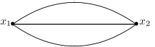
Figure 2. Caterpillar genus $2$.

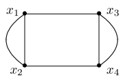
Figure 3. Caterpillar genus $3$.

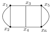
Figure 4. Caterpillar genus $4$.

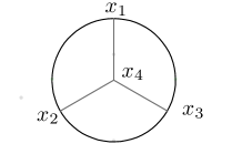
Figure 5. Star graph $K_{1,3}$.

degree d	Caterpillar genus 2			Caterpillar genus 3
	Singular-1	Singular-2	OSCAR	Singular-1	Singular-2	OSCAR
1	0.01	0.01	0.00001	0.10	0.10	0.0003
2	0.70	0.02	0.00006	0.74	0.35	0.001
3	1.23	0.021	0.0001	10.20	0.78	0.004
4	10.21	0.030	0.00016	72.41	1.54	0.012
5	51.84	0.032	0.0002	343.03	2.76	0.03
6	173.94	0.041	0.0003	1300	4.72	0.68
7	345.16	0.044	0.00035	4030	7.94	0.14
8	570.06	0.051	0.0004	–	13.6	0.26
9	819.31	0.053	0.0005	–	23.9	0.47
10	1060	0.06	0.0007	–	41.9	0.82
11	1287	0.07	0.0007	–	72.3	1.35
12	1386	0.08	0.0010	–	122	2.24
13	1714	0.09	0.0011	–	211	3.48
14	2433	0.10	0.0014	–	351	5.62
15	3376	0.11	0.0015	–	559	8.49
16	4390	0.12	0.0018	–	940	12.9
17	–	0.14	0.0019	–	1 450	20.7
18	–	0.15	0.0023	–	2 300	27.6
19	–	0.17	0.0024	–	3 440	40.5
20	–	0.19	0.0029	–	5 130	58.7

Table 1. Timings for caterpillar source curves of genus 2 and genus 3.

degree d	Caterpillar genus 4			Star graph $K_{1,3}$
	Singular-1	Singular-2	OSCAR	Singular-1	Singular-2	OSCAR
1	32.16	8.24	0.021	0.08	0.17	0.0007
2	4016	35.0	0.12	1.20	0.42	0.003
3	–	136	0.83	18.1	0.92	0.012
4	–	2240	5.53	124	1.77	0.039
5	–	32 890	29.0	549	3.19	0.112
6	–	–	121	1 990	5.80	0.27
7	–	–	419	6 080	10.3	0.56
8	–	–	2 420	18 200	19.7	1.10
9	–	–	3 490	–	38.0	1.94
10	–	–	38 700	–	72.0	3.21
11	–	–	–	–	130	5.28
12	–	–	–	–	238	8.50
13	–	–	–	–	424	13.8
14	–	–	–	–	716	20.2
15	–	–	–	–	1 190	28.6
16	–	–	–	–	1 880	40.8
17	–	–	–	–	2 970	57.3
18	–	–	–	–	4 777	79.2
19	–	–	–	–	7 103	107
20	–	–	–	–	10 620	144

Table 2. Timings for caterpillar genus 4 and $K_{1,3}$ source curves.

  

  

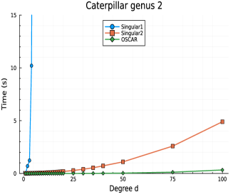
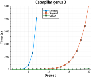
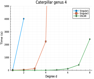
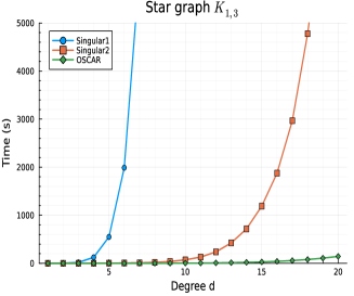
Figure 4. Visualization of the timings for Singular-1, Singular-2, and OSCAR.

  

  

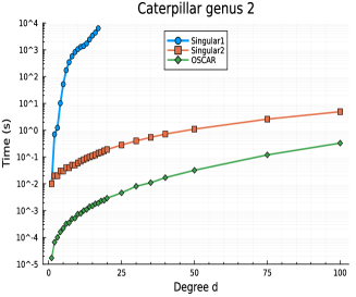
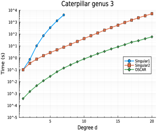
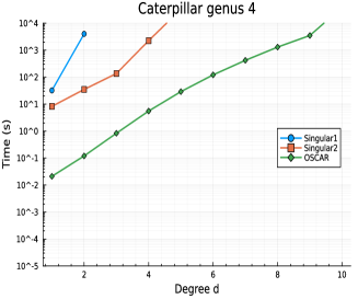
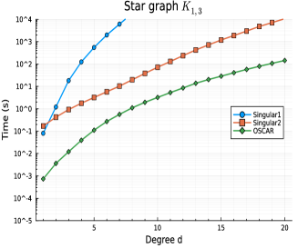
Figure 5. Visualization of the timings for Singular-1, Singular-2, and OSCAR (logarithmic time scale).

4.1. Example Computation

In this section, we provide example code for computing the Hurwitz nunmers for a caterpillar genus $3$ source curve.

⬇

julia> using GromovWitten

julia> G = FeynmanGraph([(1, 3), (1, 2), (1, 2), (2, 4), (3, 4), (3,4)] )

graph([(1, 3), (1, 2), (1, 2), (2, 4), (3, 4), (3, 4)])

julia> F = FeynmanIntegral(G)

julia> a = [0, 2, 1, 0, 0, 1];

julia> feynman_integral_branch_type(F, a)

256*q[2]^4*q[3]^2*q[6]^2

julia> feynman_integral_degree(F, 3)

288*q[1]^3 + 32*q[1]^2*q[2] + 32*q[1]^2*q[3] + 32*q[1]^2*q[5] + 32*q[1]^2*q[6] + 8*q[1]*q[2]*q[5] + 8*q[1]*q[2]*q[6] + 8*q[1]*q[3]*q[5] + 8*q[1]*q[3]*q[6] + 24*q[2]^3 + 152*q[2]^2*q[3] + 8*q[2]^2*q[5] + 8*q[2]^2*q[6] + 152*q[2]*q[3]^2 + 32*q[2]*q[3]*q[5] + 32*q[2]*q[3]*q[6] + 32*q[2]*q[4]^2 + 8*q[2]*q[4]*q[5] + 8*q[2]*q[4]*q[6] + 8*q[2]*q[5]^2 + 32*q[2]*q[5]*q[6] + 8*q[2]*q[6]^2 + 24*q[3]^3 + 8*q[3]^2*q[5] + 8*q[3]^2*q[6] + 32*q[3]*q[4]^2 + 8*q[3]*q[4]*q[5] + 8*q[3]*q[4]*q[6] + 8*q[3]*q[5]^2 + 32*q[3]*q[5]*q[6] + 8*q[3]*q[6]^2 + 288*q[4]^3 + 32*q[4]^2*q[5] + 32*q[4]^2*q[6] + 24*q[5]^3 + 152*q[5]^2*q[6] + 152*q[5]*q[6]^2 + 24*q[6]^3

julia> f = feynman_integral_degree_sum(F, 3)

288*q[1]^6 + 32*q[1]^4*q[2]^2 + 32*q[1]^4*q[3]^2 + 32*q[1]^4*q[5]^2 + 32*q[1]^4*q[6]^2 + 8*q[1]^4 + 8*q[1]^2*q[2]^2*q[5]^2 + 8*q[1]^2*q[2]^2*q[6]^2 + 8*q[1]^2*q[3]^2*q[5]^2 + 8*q[1]^2*q[3]^2*q[6]^2 + 24*q[2]^6 + 152*q[2]^4*q[3]^2 + 8*q[2]^4*q[5]^2 + 8*q[2]^4*q[6]^2 + 152*q[2]^2*q[3]^4 + 32*q[2]^2*q[3]^2*q[5]^2 + 32*q[2]^2*q[3]^2*q[6]^2 + 8*q[2]^2*q[3]^2 + 32*q[2]^2*q[4]^4 + 8*q[2]^2*q[4]^2*q[5]^2 + 8*q[2]^2*q[4]^2*q[6]^2 + 8*q[2]^2*q[5]^4 + 32*q[2]^2*q[5]^2*q[6]^2 + 8*q[2]^2*q[6]^4 + 24*q[3]^6 + 8*q[3]^4*q[5]^2 + 8*q[3]^4*q[6]^2 + 32*q[3]^2*q[4]^4 + 8*q[3]^2*q[4]^2*q[5]^2 + 8*q[3]^2*q[4]^2*q[6]^2 + 8*q[3]^2*q[5]^4 + 32*q[3]^2*q[5]^2*q[6]^2 + 8*q[3]^2*q[6]^4 + 288*q[4]^6 + 32*q[4]^4*q[5]^2 + 32*q[4]^4*q[6]^2 + 8*q[4]^4 + 24*q[5]^6 + 152*q[5]^4*q[6]^2 + 152*q[5]^2*q[6]^4 + 8*q[5]^2*q[6]^2 + 24*q[6]^6

julia> substitute(f)

1792*q[1]^6 + 32*q[1]^4

References

- [1] Firoozeh Aga, Janko Böhm, Alain Hoffmann, Hannah Markwig, and Ali Traore. GromovWitten.jl. An OSCAR-based package computing Gromov-Witten invariants of elliptic curves. https://github.com/singular-gpispace/GromovWitten, 2023.
- [2] Kai Behrend. Gromov-Witten invariants in algebraic geometry. Invent. Math., 127(3):601–617, 1997.
- [3] Kai Behrend and Barbara Fantechi. The intrinsic normal cone. Invent. Math., 128:45–88, 1997.
- [4] Benoît Bertrand, Erwan Brugallé, and Grigory Mikhalkin. Tropical open Hurwitz numbers. Rend. Semin. Mat. Univ. Padova, 125:157–171, 2011.
- [5] Janko Böhm, Kathrin Bringmann, Arne Buchholz, and Hannah Markwig. Tropical mirror symmetry for elliptic curves. J. Reine Angew. Math., 732:211–246, 2017.
- [6] Janko Böhm, Kathrin Bringmann, Arne Buchholz, and Hannah Markwig. ellipticcovers.lib. A Singular 4 library for Gromov-Witten invariants of elliptic curves, 2018.
- [7] Janko Böhm, Christoph Goldner, and Hannah Markwig. Counts of (tropical) curves in and Feynman integrals. Ann. Inst. Henri Poincaré D, 9(1):121–158, 2022. Preprint, arXiv:1812.04936.
- [8] Janko Böhm, Christoph Goldner, and Hannah Markwig. Tropical mirror symmetry in dimension one. SIGMA, 18:046, 2022. Preprint, arXiv:1809.10659.
- [9] Renzo Cavalieri, Paul Johnson, and Hannah Markwig. Tropical Hurwitz numbers. J. Algebr. Comb., 32(2):241–265, 2010. arXiv:0804.0579.
- [10] Renzo Cavalieri, Paul Johnson, Hannah Markwig, and Dhruv Ranganathan. A graphical interface for the Gromov-Witten theory of curves. In Algebraic geometry: Salt Lake City 2015, volume 97 of Proc. Sympos. Pure Math., pages 139–167. Amer. Math. Soc., Providence, RI, 2018.
- [11] Renzo Cavalieri and Eric Miles. Riemann surfaces and algebraic curves, volume 87 of London Mathematical Society Student Texts. Cambridge University Press, Cambridge, 2016. A first course in Hurwitz theory.
- [12] Robbert Dijkgraaf. The moduli space of curves, volume 129 of Progr. Math., chapter Mirror symmetry and elliptic curves, pages 149–163. Birkhäuser Boston, 1995.
- [13] Mark Gross and Bernd Siebert. Mirror Symmetry via logarithmic degeneration data I. J. Differential Geom., 72:169–338, 2006. arXiv:math.AG/0309070.
- [14] Robin Hartshorne. Algebraic Geometry. Springer, 1977.
- [15] Si Li. BCOV theory on the elliptic curve and higher genus mirror symmetry. Preprint, arXiv:1112.4063, 2011.
- [16] Grigory Mikhalkin. Enumerative tropical geometry in . J. Amer. Math. Soc., 18:313–377, 2005.
- [17] Andrei Okounkov and Rahul Pandharipande. Gromov-Witten theory, Hurwitz theory, and completed cycles. Ann. of Math., 163(2):517–560, 2006.
- [18] Ravi Vakil. The moduli space of curves and Gromov–Witten theory. In Enumerative invariants in algebraic geometry and string theory, pages 143–198. Springer, 2008.