The fluid mechanics of splat painting
Abstract
In splat painting, a collection of liquid droplets is projected onto the substrate by imposing a controlled acceleration to a paint-loaded brush. To unravel the physical phenomena at play in this artistic technique, we perform a series of experiments where the amount of expelled liquid and the resulting patterns on the substrate are systematically characterized as a function of the liquid viscosity and brush acceleration. Experimental trends and orders of magnitude are rationalized by simple physical models, revealing the existence of an inertia-dominated flow in the anisotropic, porous tip of the brush. We argue that splat painting artists intuitively tune their parameters to work in this regime, which may also play a role in other pulsed flows, like violent expiratory events or sudden geophysical processes.
1 Introduction
Painting is one of the earliest human artistic expressions. Early cave paintings are considered by many the signature for the emergence of human behavior [1]. A series of recent papers have argued that the essence of artistic painting lays within a keen understanding of the physical constraints imposed by the interaction between the artist, their instruments and materials [2, 3, 4, 5]. In other words, artists develop a deep physical knowledge on how to manipulate fluid flows to paint. They skillfully choose tools, paints and action to cover canvases with certain fluid textures in order to convey their intention to the painting.
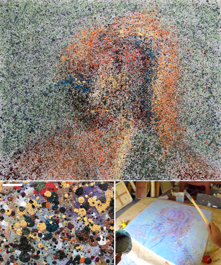
In this paper we study the splat painting technique. It consists in subjecting a paint-loaded brush to a sudden acceleration, for example by “flicking” the brush or tapping its handle. As a result, the paint is expelled from the brush, producing droplets or filaments that then are projected onto a canvas, leaving fragmented patterns [2]. Figure 1 displays an example of a modern artwork created with splat painting ; video S1 shows the process in action. In this technique, perhaps most emblematically used by American painters Jackson Pollock (1912-1956) [5] and Sam Francis (1923-1994) [6], the brush never touches the canvas. Splat painting is thus considered an action painting technique. This term, coined by Harold Rosenberg [7], refers to the use of dribbling, splashing or smearing paint onto a canvas. Its relevance, discussed by many art historians and critics, emerges from the fact that the creation process is not entirely under the control of the artist; the deposition of paint on the canvas is governed by the mechanical constraints of the process rather than the will of the artist. In this sense, Rosenberg argued that art could be redefined to include the act rather than just the object, as a process rather than a product. In the absence of contact between the brush and the substrate, paint composition becomes one of the main leverages to tune the production of droplets and their final deposition. The artist therefore develops a certain intuition on how the physical properties of the paint (mostly viscosity) should be adjusted to obtain a desired effect.
The splat painting technique can be conceptualized as being the sequence of the following physical processes. First, the brush is loaded with paint. A certain volume of paint can be retained inside the bundle of bristles without dripping due to a capillary effects [8, 9]. Once loaded, the brush is flicked, either by rapid hand motion or a gentle tap. The sudden motion accelerates the tip of the brush, causing the fluid trapped within the bristles to flow and eventually leave the brush. Acceleration-driven ejection of liquid can be encountered in a variety of contexts. In nature, wet mammals shake [10] and insects flutter their wings [11] at given frequencies to get rid of excessive moisture or droplets. In industrial processes, the rotary atomization of liquids submitted to centrifugal acceleration is commonly used to produce droplets or sprays (see [12] and references therein). Once the fluid is ejected from the bristle bundle, it forms filaments that fly away. In most cases, these filaments fragment into droplets due to the classical Rayleigh-Plateau instability [13]. The droplets finally land on the canvas to create the artist composition, as illustrated in Fig. 1. Droplet impact on a substrate has been extensively studied [14, 15], due to its importance in many engineering applications and natural phenomena, from inkjet printing [16] to pathogens transmission [17].
The process of splat painting is clearly a rich fluid mechanical problem. While some aspects of its mechanics have been addressed by other studies, a specific investigation that focuses on the parameters relevant to this artistic painting technique does not exist. To unravel the physical mechanisms at play in splat painting, we performed experiments on a setup allowing us to impose a controlled acceleration to a liquid-loaded brush (see Methods section). Varying the paint viscosity and brush acceleration, we are then able to rationalize the effect of these parameters on the amount of liquid ejected (section 2) and on the resulting spotted pattern (section 3).
2 How much liquid is ejected?
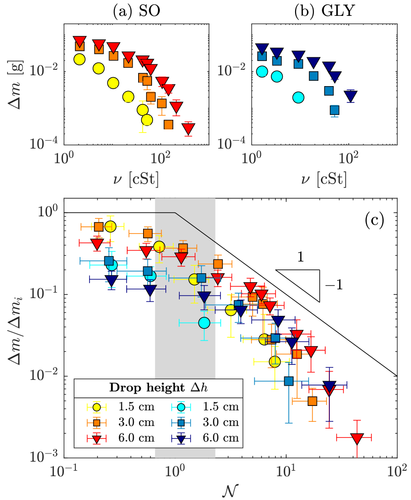
Experimentally, the acceleration is produced by dropping a weight (impactor) from a given height , onto the brush handle. The liquid mass ejected from the bundle is measured as a function of the liquid kinematic viscosity for various impactor drop heights. For both silicone oils (SO, figure 2a) and water-glycerol mixtures (GLY, figure 2b), and regardless of , two regimes are observed depending on the viscosity. At low viscosities, seems to plateau out toward a constant value while, at larger viscosities, the mass decays with following a trend compatible with a power law. In the following, we propose to rationalize those two regimes by modelling the acceleration-driven flow in the brush bundle.
2.1 Brush kinematics
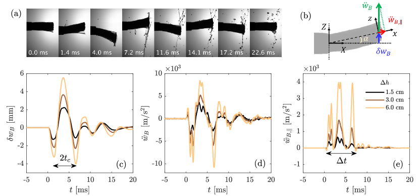
How the impact from a given height translates into the brush motion is a complex solid mechanical problem, which we do not aim to address here. Instead, we focus directly on the kinematics of the brush upon impact, as revealed by high-speed imaging (see supplementary movie S2 and figure 3a). In order to quantify the movement of the brush, we introduce in Figures 3b and 7 the coordinate system tied to the (non-inertial) reference frame of the accelerated brush handle. Digital image processing of sequences such as Figure 3a allows us to measure vertical displacements in the reference frame of the laboratory: for the rigid handle, and for the deformable bundle. The bundle vertical displacement relative to the handle, that is to say its deflection with respect to its equilibrium position, is defined as (Figure 3c). Additionally, the vertical displacement is time-differenciated twice to obtain the instantaneous vertical acceleration of the bundle (Figure 3d) in the reference frame of the laboratory.
2.2 Driving mechanism
In our experimental conditions, we observe that liquid is predominantly ejected from the tip of the bundle, as shown in figure 3a. Assuming an initially uniform liquid distribution in the bristles, this observation implies that the vertical forcing mostly drives liquid along the bundle to the tip, where it detaches and fragments. This is due to the combination of two key ingredients.
First, at each point along the central line of the bundle, the local, vertical forcing acceleration can be divided into a transversal and a longitudinal component (Figure 3b). Because of the top-down symmetry of the motion, the former averages out to zero over several oscillation cycles, while the latter, denoted , imposes a forcing with non-zero average to the fluid. Observing that the deflection angle (see figure 3b) is roughly uniform along the bundle, the projected acceleration can be approximated as , under the assumption that . As shown in Figure 3e, the projected acceleration is positive during most of the motion, indeed pushing the liquid towards the bundle tip.
Second, as can be estimated from the anisotropic bundle geometry (see appendix A), the transversal permeability (i.e. in the radial direction ) is about 5 times smaller than the longitudinal one [18]. Is is therefore easier for the liquid to move in the longitudinal direction compared to the radial one. Combining these two arguments, we arrive at the conclusion that the flow of paint in the bundle mainly takes place in the direction parallel to the bristles and that the main driving force is the longitudinal projection of the bundle acceleration.
2.3 Flow regimes in the bundle
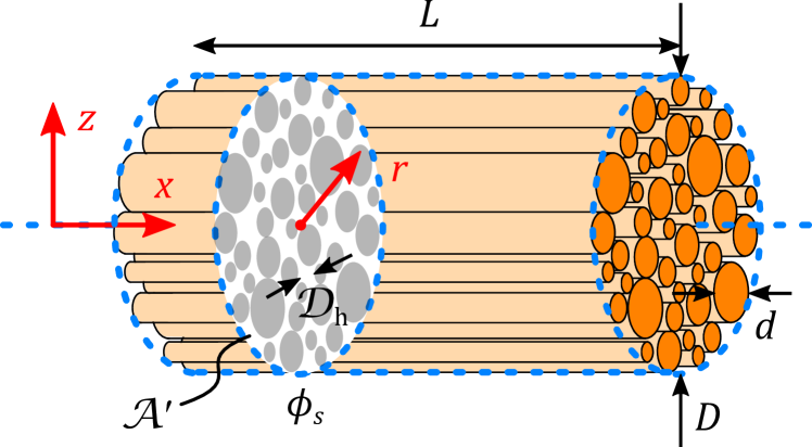
As can be appreciated in Figure 3a, the wet bundle keeps a roughly cylindrical shape of diameter during its oscillations. We therefore model it as cylindrical slab of porous material of diameter and length (Figure 4), in which all the pores (the spaces between fibers) are assumed to be parallel. Measuring experimentally the values of , , as well as the distribution of bristle diameters , we are able to determine the solid fraction and typical pore diameter to be assigned to the idealized bundle (see appendix A).
Let us now write an equation of motion for the incompressible and Newtonian liquid flowing in this model bundle. Momentum conservation applied in the (non-inertial) reference frame of the bundle reads
| (1) |
where is the (three-dimensional) fluid velocity, the pressure and the linear (vertical) bundle acceleration in the reference frame of the laboratory.
Equation (1) is then projected onto the longitudinal direction of the bundle, which is expected to be the main flow direction. Additionally, the characteristic lengthscale in the transversal direction is the hydraulic diameter of the pores between the bristles, , while the one in the longitudinal direction is the bundle length . Under the approximation of slender flow and using the coordinate system tied to the bundle (Figure 4), we arrive at
| (2) |
where and denote the components of the fluid velocity in the longitudinal and radial directions, respectively.
The characteristic timescale , defined as the average half-period of the bundle oscillations, and characteristic longitudinal acceleration, , can be estimated from the brush kinematics (see figure 3 and appendix B). Typical values are and , depending on the drop height . The velocity scale of the flow in the bundle remains a priori unknown and will be set by the dominant force balance in equation (2).
The fate of the momentum injected by the impact (last term in equation (2)) is mostly to accelerate the liquid and to be dissipated by viscous friction. Which of these mechanisms is dominant depends on the ratio between the viscous term (second on right-hand side) and the transient inertial term (first in left-hand side) in equation (2), quantified by the dimensionless number
| (3) |
Note that for a periodic flow, this parameter would be equivalent to the Womersley number . In our setting, we simply refer to as the dimensionless viscosity. Experimentally, , therefore requiring to discuss both the inertia-and viscosity-dominated regimes.
For , the forcing acceleration is mostly used to accelerate the liquid through the transient term of equation (2). This leads to a typical velocity scale
| (4) |
of the order of a few . Note that, in this regime, the value of the Strouhal number , comparing the transient to convective inertial terms, is of the order of a few units. Convective effects are therefore expected to be subdominant.
For , the forcing acceleration is mostly dissipated by viscous friction, leading to a typical velocity scale
| (5) |
2.4 Modelling the ejected mass
Knowing the characteristic flow velocity in the different regimes, the total mass expelled from the brush can be estimated as
| (6) |
where is the liquid flow rate going through the bundle and the total duration of impact, typically in the range (see appendix B). The flow rate is simply expressed as , where is the total cross-sectional area available for the fluid to flow in the bundle, computed from its geometry (see appendix A). Combining equation (6) with the characteristic velocities in the different regimes (equations (5) and (4)), we arrive at
| (7) | ||||
| (8) |
in the inertial and viscous limits, respectively.
The predictions of equations (7) (for ) and (8) (for ) are shown in figure 2c (solid line). Experimental masses are made dimensionless with the predicted detached mass in the inertial limit (equation (7)) and plotted as a function of the dimensionless viscosity (equation (3)). Comparison between the non-dimensionalized data (symbols) and the predictions of the scaling analysis shows an overall good agreement, both in trend and orders of magnitude. For a given liquid family (SO or GLY), the dimensionless data corresponding different drop heights do collapse onto a single mastercurve. Interestingly, the mastercurves for SO and GLY overlap in the viscous regime () but depart slightly in the inertial regime (). This discrepancy is likely due to capillary effects, as the typical surface tension of water-glycerol is more than 3 times larger than the one of silicone oils (see appendices C and D). The shaded area in figure 2c shows the range of dimensionless viscosities corresponding to artist-chosen splat painting conditions with acrylic paint (see appendix E). Strikingly, those values are located around , suggesting that artists dilute their paint and/or adjust their tapping strength to work close to the inertia-dominated regime.
3 How is liquid distributed on the substrate?
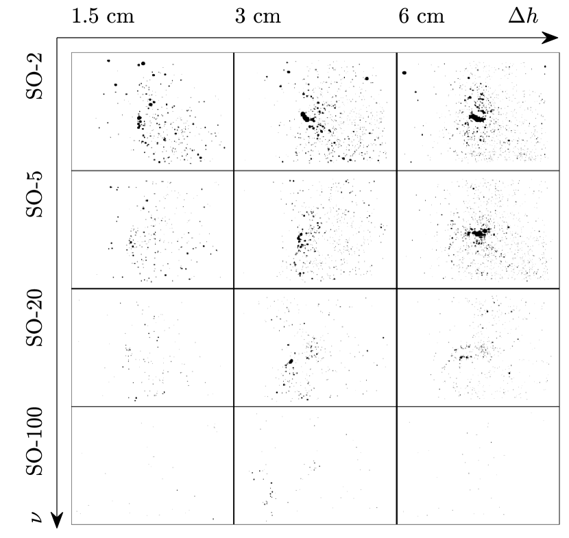
Of paramount importance in the context of artistic painting is the final spotted pattern obtained on the substrate (see figure 1 and videos S1). Figure 5 shows examples of the patterns generated in our experimental conditions for a selection of drop heights and silicone oil kinematic viscosities . Given an initial mass of liquid expelled from the brush, those patterns are the result of a complex interplay between (i) liquid fragmentation, (ii) drop flight dynamics and (iii) droplet impact dynamics on the substrate. Each of these processes is the subject of a whole body of literature on its own. We will therefore simply focus on key ideas allowing us to draw a connection between the total painted area (sum of all the black areas for a given pattern in figure 5) and the ejected mass , which was rationalized in the previous section.
3.1 Liquid fragmentation
Once the fluid is expelled from the brush, the elongation of fluid filaments leads to fragmentation and droplet formation. The droplet size distribution resulting from this complex process has been abundantly studied in the literature [13], including under radial (centrifugal) acceleration conditions [19, 12]. Although this distribution is not quantified in our experiments, a typical drop diameter can be estimated, based on the idea that the expelled liquid filaments leave the brush with a diameter of the order of the pore size in the bundle. Subsequent filament destabilization under the action of the Rayleigh-Plateau instability does not modify this length scale substantially [20]. For the sake of simplicity, we will henceforth assume that the droplet population resulting from splat painting consists of identical drops of diameter , with .
3.2 Drop flight dynamics
Considering a droplet of diameter leaving the brush with an initial velocity at a height above the substrate, we wish to estimate its velocity at the moment of its impact on the substrate. Approximating the initial drop velocity by the typical (vertical) velocity of the tip of the bundle in the reference frame of the laboratory, is found experimentally to be of the order of , depending on . The impact velocity of the droplet then depends on how much it was slowed down by air friction during its flight. This can be quantified comparing the flight time of the droplet and the characteristic time of viscous friction in air (see appendix F). In our experimental conditions, we can show that for droplets leaving the brush with a vertical velocity pointing downwards, which is the situation leading to the shortest flight time. The impact velocity on the substrate may therefore be approximated terminal velocity of the droplet in air.
3.3 Drop impact
The impact dynamics of a drop on a solid surface is essentially governed by the Weber and Reynolds numbers [14, 15], defined respectively as
| (9) |
In particular, those parameters control the maximum lateral extension of the impacting drop (or maximum spreading diameter ) [21] and the occurrence of splashing (i.e. fragmentation of the drop upon impact) [15], that happens for . Across the whole parameter space covered in our experiments, we estimate , , and in the limit of a drop impacting at its terminal velocity (, see appendix F). We therefore do not expect the impacting drops to undergo splashing, as confirmed by visual inspection of the patterns.
For a drop impacting on a rough surface like paper, no rebound or recoil can happen as the contact line remains pinned to the substrate [22]. Consequently, the maximum spreading diameter can be considered a good approximation for the diameter of the spot left on the paper.
3.4 Modelling the total painted area
Taking advantage of the abovementionned simplifications, we now set out to find a relationship between the detached mass and the total painted area . The volume corresponding to identical drops of diameter is , which is experimentally measured as . Making the additional assumption that the spots left by the droplets on the substrate do no overlap, the total painted area can be written as , where denotes the diameter of a spot. Combing those expressions and recalling that , we obtain
| (10) |
where we have introduced the drop spreading factor . Scaling by the prediction in the inertial limit (equation (7)) leads to
| (11) |
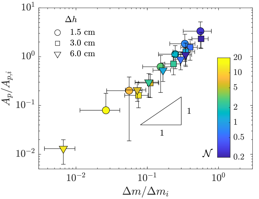
where the total painted area is made dimensionless with .
Figure 6 reveals that the dimensionless painted areas and detached masses, obtained experimentally for silicone oils of various viscosities splatted onto paper, are proportional. The drop spreading factor is therefore roughly constant in our experiments. This is compatible with predictions [15] showing that is only a weak function of the impact parameters (Weber number and Reynolds number ). More quantitatively, fitting the data of figure 6 with equation (11) yields a typical drop spreading factor of . This value is consistent with the one expected for [21].
4 Conclusion
In summary, we investigated the artistic technique of splat painting from a fluid mechanical perspective. Inspired by the empirical know-how developed by artists, we explored the influence of two key parameters – liquid viscosity and brush acceleration – on the quantity of liquid ejected from the brush and on the final spotted pattern laid down on the substrate.
We showed that the amount of liquid leaving the brush exhibits two regimes, depending on the value of the dimensionless parameter that compares viscous dissipation to liquid inertia in the hair bundle. For , most of the brush’s momentum is dissipated by viscosity and the detached mass is proportional to the Stokes number. For , the brush’s momentum is mostly used to accelerate the paint and the expelled mass tends to its upper limit, which is independent of . The viscosities of acrylic paint solutions used for splat painting correspond to this inertia-dominated regime, while native acrylic paint would fall within the viscous-dominated regime. We thus argue that artists dilute their paint to perform splat painting (i.e. decrease ) until they reach the inertial regime , which allows them to maximize the expelled mass. Additionally, we evidenced that the total paint-covered area on the substrate is essentially proportional to the detached mass: drop spreading upon impact does not contribute significantly to the spot size. The total area covered is therefore essentially governed by the flow in the bundle, which sets the amount of liquid expelled, and not by the drop impact conditions on the substrate (at least in the absence of slippage).
Materials and methods
Materials
Brush
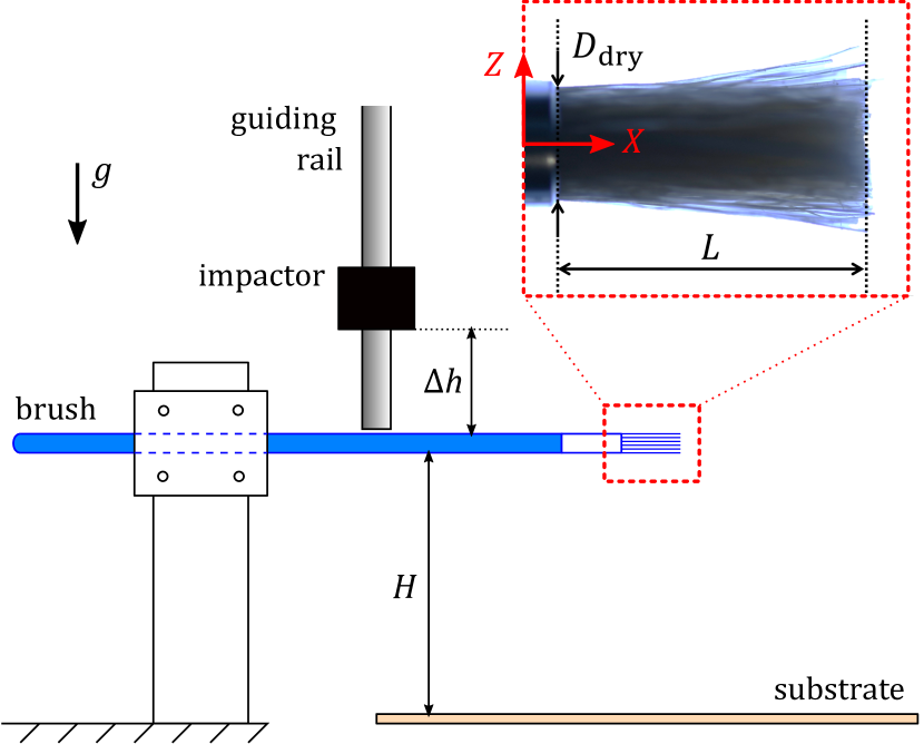
In our experiments, we use a set of identical commercial round brushes, purchased from a local crafts shop. Each brush is composed of a wooden handle connected to a bundle of natural hairs (also called bristles) by a metallic ferrule. The only modification we make to this brush is to trim the tip of the bundle, cutting all the bristles to a uniform length (see close-up in figure 7). At the exit of the ferrule, the dry bundle has a diameter . Examination under the microscope reveals that the hairs are quite polydisperse, with an average diameter (std), see appendix A. We will henceforth assume that all our brush copies share these same properties.
Liquids
Most paints are non-Newtonian fluids, exhibiting shear-thinning, yield-stress or even viscoelastic properties [24, 25]. However, to be able to vary the fluid shear viscosity independently from the brush acceleration (and therefore shear rate), we choose to focus our study on Newtonian liquids. Two families of Newtonian liquids are used: silicone oils, denoted by prefix SO, and water-glycerol mixtures, denoted by prefix GLY. Both these families allow us to vary viscosity over three orders of magnitudes while keeping density and surface tension roughly constant (see appendix C).
Substrate
The substrate on which splatted liquid droplets are collected is A4 white paper (, Navigator). The distance between the brush and the substrate is set to a constant value throughout all the experiments.
Experimental setup and protocol
Impact setup
We developed a custom-made experimental setup to mimic the conditions in which an artist accelerates the paint-loaded brush to produce splat patterns. As shown in figure 7, the brush is held horizontally at a fixed height above the substrate. The wooden handle is clamped to simulate how the painter would hold the brush. Brush acceleration is generated by dropping onto the wooden handle a ring-shaped brass weight guided along a fixed vertical brass tube. The impact generates a transverse wave that propagates in the handle all the way to the tip of the brush, where it is transmitted to the paint-loaded bristles. The magnitude of the maximum acceleration can be adjusted by changing the height from which the weight is dropped (see appendix B). Three drop heights are reported in this study: , and .
Measurement setup and protocol
The brush is initially loaded with a fixed mass of liquid , which is kept constant throughout the experiments. We also make sure that the clamping of the handle and impact location are the same for all experiments.
During impact, the vertical displacements of the extremity of the handle and of the bristles, as well as the resulting liquid atomization, are visualized from the side and recorded by a high-speed camera (NAC MEMRECAM HX 3) at a framerate of 30,000 fps. A typical image sequence is presented in Fig. 3a. In-house image processing is subsequently used to extract displacements and accelerations.
The total mass of liquid ejected is measured by weighting the brush before and after impact with a high-precision scale (Sartorius, resolution ). In addition, for a selection of silicone oils, the ejected droplets resulting from the tapping are collected on the substrate laid down horizontally at a fixed distance below the brush. Immediately after splatting ( after impact), a top view of the final drop pattern is photographed using a Samsung Galaxy S20 camera (resolution of 12 megapixels) and backlighting with a homogeneous light panel (dimensions ).
Image processing of patterns
Photographs of the patterns are subsequently processed using an in-house Matlab code. Under backlighting conditions, the silicone oil drops on paper appear as bright spots on a darker background. Spot detection is therefore performed through image binarization, using an adaptive threshold. However, due to the heterogeneity of the paper substrate, the background itself features some granularity. The resulting spurious spots are filtered out using as a reference the photograph of the blank paper under the same imaging conditions. Examples of the final processed patterns are shown in Figure 5.
Acknowledgments
J.R.R. acknowledges funding from the Spanish MCIN/AEI/10.13039/501100011033 through Grant No. PID2020-114945RB-C21. This project has received funding from the European Union’s Horizon 2020 research and innovation programme under the Marie Sklodowska-Curie grant agreement No 882429 (L.C.). We are very grateful to splat paiting artists Octavio Moctezuma and Caroline Champougny for sharing their expertise on this technique, as well as their paint recipes. Many thanks as well to Mithun Ravisankar for his help with the rheological measurements of paints.
Appendix A Bundle geometry
In this section, we characterize experimentally the geometry of brush’s hair bundle. We then deduce and discuss geometrical properties of the anisotropic porous medium used as an idealized representation of the bundle. The values of the most important properties are summarized in table 1.
| Property | Value | Eq. |
|---|---|---|
| Wet diameter | - | |
| Solid fraction | (14) | |
| Hydraulic diameter | (16) | |
| Permeability ratio (squ.) | (19) | |
| Permeability ratio (hex.) | (19) |
A.1 Bristle diameter distribution
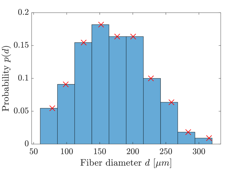
To determine geometrical properties such as bristle number and bristle diameter distribution, the bundle of one of the brush copies is severed at its base to be characterized. The total number of hairs in the bundle is determined by weighting several known amount of hairs on a high precision scale (Sartorius, with a resolution of ). Measuring the total mass of all the bristles then allows us to deduce their number, which is found to be . A reduced sample of hairs from the brush (about of the total) is examined under the microscope to measure their diameter distribution.
The experimental probability distribution of bristles’ diameters is presented in figure 8. This distribution is characterized by its first and second moments, defined respectively as
| (12) | ||||
| (13) |
where is the number of bins used to compute the probability distribution, and the average diameter in bin (red crosses in figure 8). Assuming that the bristles’ diameters in the idealised bundle follow the same distribution (i.e. have the same and ), we are able to compute the following properties of the model porous medium.
A.2 Solid fraction
The solid volume fraction is defined as the total volume occupied by the fibers, normalized by the total volume of the bundle. Denoting the total cross-sectional area of the bundle, we have
| (14) |
where we recall that is the total number of fibers in the bundle and the diameter of the liquid-loaded bundle. The corresponding estimation of the bundle’s solid fraction is provided in table 1.
A.3 Hydraulic diameter
The hydraulic diameter of the bundle is defined as
| (15) |
where is the total cross-sectional area available for the liquid to flow and is the total wet perimeter in the bundle. Eventually, the hydraulic diameter can be expressed as
| (16) |
where we took advantage of equation (14) to replace . Note that, in the case of a bundle of identical fibers of radius , the quantity reduces to and we find the expression proposed by Gebart [26]. For the diameter distribution presented in figure 8, we estimate the hydraulic diameter to be of the order of a hundred microns (see table 1).
A.4 Permeabilities
An anisotropic porous medium (such as the one depicted in figure 4 of the main text) has different permeabilities, depending if the flow is parallel or perpendicular to the fiber direction. For a bundle of identical fibers of radius , Gebart [26] derived analytical expressions for the longitudinal and transversal permeabilities, denoted and , respectively:
| (17) | ||||
| (18) |
where , and are constants that depend on the geometry of the fiber packing. For a square packing, , and , while for a hexagonal packing , and . Interestingly, the ratio between the longitudinal and transversal permeabilities is independent of the fiber radius :
| (19) |
To the best of our knowledge, there are no expressions equivalent to equations (17), and (18) in the literature for a bundle of polydisperse fibers. However, since equation (19) does not depend on the fiber radius, we may compute the permeability ratio for a monodisperse bundle with the same solid fraction as our polydisperse bundle. The corresponding values are reported in table 1 for two possible ordered fiber packing geometries (square and hexagonal).
Assuming that the permability ratios estimated in the monodisperse case provide a reasonable order of magnitude for the polydisperse case (for a given solid fraction), we expect the longitudinal permeability to be about 5 times larger than the transversal one for our brush’s bundle.
A.5 Effect of liquid loading
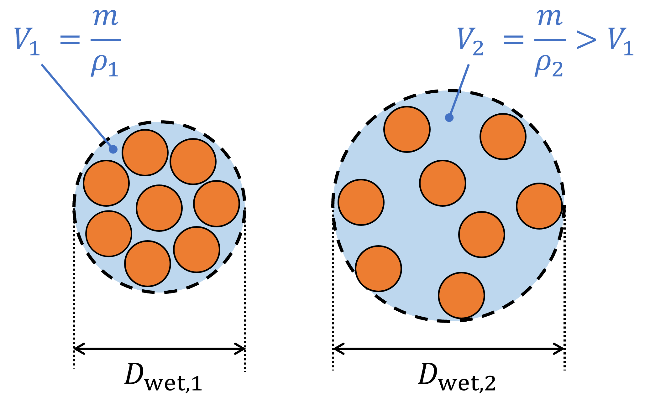
When a hairy structure is wet, capillary forces tend to bring the hairs closer together, an effect that is referred to as clumping [27, 9, 8, 28, 29]. This is the reason why the brush bundle is tighter when it is wet as compared to when it is dry (Figure 10). Because liquids are incompressible, we expect that the diameter of the wet bundle depends on the volume of liquid loaded on it (as long as there is no dripping). However, our protocol involves loading a fixed mass of liquid in the bundle. Since density can vary up to between our liquids (see table 3), the loaded volume and therefore the wet diameter may vary slightly between experiments, as illustrated in Figure 9.
In the following, we show how the bundle geometrical properties can be corrected for this effect. Volume conservation of the bundle imposes that
| (20) |
where we recall that is the cross-sectional occupied by the bristles. The cross-sectional area available for the liquid to flow is then simply be expressed as
| (21) |
and the hydraulic diameter is deduced from equation (15).
Let us assume we know the wet diameter of the bundle loaded with a given mass of a reference liquid of density . Since the bundle is always loaded with the same mass , then its geometry (i.e. available cross-sectional area and hydraulic diameter) can be straightforwardly deduced for all liquids from the reference measurement:
| (22) | ||||
| (23) |
Table 1 shows the geometrical of the bundle loaded with a mass of the reference liquid, chosen to be silicone oil (SO-1000). The available cross-sectional area and hydraulic diameter were deduced for all the other liquids in table 3 using equations (22) and (23), and used to non-dimensionalize the data in presented in Figure 2c of the main text.
Appendix B Brush impact characteristics
| Liquid family | () | () | () | () | () | () |
|---|---|---|---|---|---|---|
| (SO) | ||||||
| (GLY) | ||||||
In splat painting, the acceleration of the liquid-loaded bristles is driving the expulsion of liquid from the bundle. However, unlike other geometries where the acceleration can be imposed (for example by setting the angular frequency of a rotating device [12]), our configuration does not allow us have a direct control over the acceleration of the brush. In our experimental set-up, the control parameter is the drop height of the weight, which determines the energy of the impact on the brush’s handle. How this translates into the accelerated motion of the bundle depends on the geometry and mechanical properties of the different parts of the brush (handle, ferrule, bundle). Our approach here is not to solve this solid mechanics problem, but rather to encapsulate it using a few key observables extracted from the high-speed imaging of the bundle motion.
Liquid detachment impedes the automatic detection of the bundle motion on the video footages (see snapshots in figure 3a of the main text). This is the reason why we use here only the experimental videos for the most viscous liquids (SO-1000 and GLY-100), for which all the liquid remains trapped between the bristles. We checked that the bundle kinematics is essentially independent of the viscosity of liquid loaded in the bristles, thus allowing us to extrapolate the results obtained on SO-1000 and GLY-100 to lower viscosities. In the following, we explain how the observables characterizing the bundle kinematics are defined and computed. Table 2 summarizes their values for the two different copies of the same brush, used for the (SO) and (GLY) families respectively.
B.1 Oscillation timescale of the bundle
The characteristic timescale of the flow is set by the oscillations of the bundle during the impact. Since both upwards and downwards flinging may cause paint detachment, we define as the average half-period of oscillation of the bundle deflection (see figure 3c in the main text).
B.2 Total duration of impact
The impact duration is defined as the total amount of time during which the longitudinal projection of the bundle acceleration takes non-zero values. In practice, we use as a threshold the average of after impact (i.e. for in the example of figure 3e in the main text). The duration is then computed as the total time during which .
B.3 Characteristic accelerations
The typical longitudinal acceleration driving the flow along the bundle is obtained from the time integral of (see figure 3e in the main text). It is defined as
| (24) |
and evaluated at the bundle tip (), where most of the liquid expulsion occurs.
Similarly, for the purpose of estimating the effective Bond number (see section D), we also define the typical vertical acceleration of the bundle as
| (25) |
where the vertical bundle acceleration is taken at .
B.4 Characteristic vertical velocity
Liquid drops and filaments leave the brush with a velocity that is equal to the one of the tip of the bundle (in the reference frame of the lab). The typical vertical velocity of a drop right after detachment can therefore be estimated as
| (26) |
where is again a proxy for the location of the bundle tip.
Appendix C Liquid preparation and properties
Experiments are carried out at ambient temperatures ranging from to , with an average . Table 3 summarizes the physical properties of all the liquids investigated at the average temperature . However, note that the values of density and viscosity are corrected to account for the actual temperature at the moment of each experiment.
C.1 Silicone oils (SO)
Silicone oils SO-2, 5, 10, 20, 50, 100, 200, 350, 1000 were used off the shelf. In addition, silicone oils SO-40, 70, 150 were obtained by blending commercially available oils using the Grunberg-Nissan mixing rule [30]. The exact kinematic viscosities of the blends were subsequently measured with an Ostwald viscometer.
C.2 Water-glycerol mixtures (GLY)
Aqueous glycerol solutions are prepared mixing pure glycerol () and ultrapure (Milli-Q) water in various proportions. Solutions are labelled GLY-, where stands for the mass fraction of glycerol in , while GLY-100 simply denotes pure glycerol. The density and viscosity of these solutions were computed based on and the ambient temperature using the correlation-based calculator developed by Andreas Volk and Chris Westbrook [31, 32].
C.3 Precautions and cleaning protocol
Silicone oils and aqueous liquids (water-glycerol and acrylic paint solutions) are tested on separate copies of the same brush. When changing the liquid on a given brush, the bristles are thoroughly cleaned, either by wiping with absorbing paper (silicone oils) or rinsing in ultrapure water and drying (aqueous liquids) to ensure the brush returns to its initial state.
Contrarily to silicone oils, water-glycerol mixtures are observed to evaporate in our experimental conditions (ambient relative humidity in the range and timescales of ). For each liquid in the GLY family, the mass lost to evaporation during the experiment, denoted , is therefore characterized experimentally. Glycerol being hygroscopic, the evaporated mass decreases when increasing the glycerol concentration, ranging from for GLY20 to values below the resolution of our scale () for GLY80. The values of the ejected mass plotted in figure 2 b of the main text are corrected from the effect of evaporation.
For each liquid family and each set of control parameters (liquid viscosity and brush acceleration), a minimum of three repetitions of the same experiments are conducted, both for mass and pattern measurements.
| Liquid code | |||
|---|---|---|---|
| SO-2 | |||
| SO-5 | |||
| SO-10 | |||
| SO-20 | |||
| SO-40 | |||
| SO-50 | |||
| SO-70 | |||
| SO-100 | |||
| SO-150 | |||
| SO-200 | |||
| SO-350 | |||
| SO-1000 | |||
| GLY-20 | |||
| GLY-40 | |||
| GLY-60 | |||
| GLY-70 | |||
| GLY-78 | |||
| GLY-80 | |||
| GLY-87 | |||
| GLY-100 |
Appendix D Effects of surface tension on the flow in the bundle
In this section, we identify and discuss three ways in which surface tension may affect (directly or indirectly) the amount of liquid ejected from the brush. The surface tension of water-glycerol solutions (GLY) is typically more than three times larger than the one of silicone oils (SO), while other properties remain similar (see table 3). These two families of liquids therefore allow us to test our hypotheses against experimental observations.
D.1 Bundle cohesion
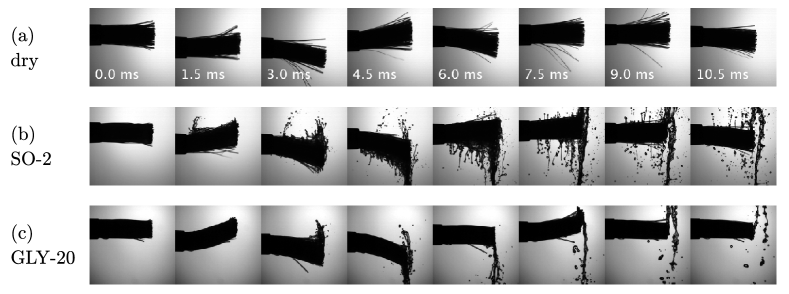
The snapshots in Figure 10a show that the wet bundle says cohesive during impact. This observation is crucial, as it allows us to define the bundle diameter and the associated bundle geometrical properties (see Appendix A).
The bundle’s cohesion is due to a combination of surface tension and viscous forces. Capillary bridges resist hair separation, as it would result in an increased interfacial area. Additionally, for two wet bristles to separate, the liquid between them must flow away, which becomes more and more difficult as viscosity increases.
Figure 10 shows that, even for the smallest viscosities tested (SO-2 on panel b, GLY-20 on panel c), the wet hair bundle remains more cohesive during impact than in the dry case (panel a). This suggests that, for both SO and GLY, capillary forces are strong enough to overcome the bristle inertia.
D.2 Transverse flow
Figure 10 also reveals differences in the phenomenology of paint detachment for low viscosity silicone oils and water/glycerol solutions. In the case of SO-2 (figure 10b), many liquid filaments are observed to detach from various locations along the “body” of the bundle, although most of the liquid still leaves from the tip. In contrast, for GLY-20 (figure 10c), which has similar viscosity and density as SO-2 but a surface tension more than 3 times larger, liquid is observed to detach exclusively from the tip of the bundle.
The effective Bond number compares the vertical inertia of the liquid to capillary forces. It can be defined as
| (27) |
where is the typical vertical bundle acceleration at its tip. For silicone oils, this number lies in the range , while for water/glycerol solutions, . Since for the SO family, the vertical acceleration is therefore strong enough to overcome surface tension and break capillary bridges at the periphery of the bundle. This results in an additional mass of liquid detached from the “body” of the bundle. On the contrary, for the GLY family, and surface tension is able to keep liquid inside the bundle along its length. Liquid thus only leaves from the bundle tip.
This mechanism may explain why, in the inertial regime () the expelled mass is systematically larger for SO as compared to GLY (see figure 2c in the main text). In the viscous regime (), liquid viscosity impedes any transverse flow in the bundle, regardless of the value of surface tension. However, in the inertial regime, the liquid can flow more easily in the transverse direction, and only a strong enough surface tension (i.e. such that ) may prevent liquid from leaving the body of the bundle.
D.3 Longitudinal capillary pressure gradient
In the framework of our scaling approach, the magnitude of capillary effects relative to the forcing longitudinal acceleration is quantified by the dimensionless surface tension
| (28) |
which is of the order of for SO and for GLY. For both liquid families, the capillary pressure gradient therefore remains only a small correction to the total pressure gradient driving the liquid in the longitudinal direction in the bundle.
Appendix E Artist-chosen splat painting conditions
In this section, we determine the range of dimensionless viscosities used in practice by splat painting artists.
| Reference | Color Name | Concentration | Kinematic viscosity | Density | Surface tension |
|---|---|---|---|---|---|
| 104 | Zinc White | ||||
| 269 | Azo Yellow Medium | ||||
| 504 | Ultramarine | ||||
| 507 | Ultramarine violet | ||||
| 735 | Oxide Black |
E.1 Acrylic paint solutions
We asked artist Caroline Champougny to prepare acrylic paint solutions suitable for splat painting. The solutions were prepared using commercial acrylic paint (Amsterdam - Standard Series, see references in table 4) of various colors diluted in ultrapure (Milli-Q) water. The procedure was the following: first, a given mass of native acrylic paint was weighted in a test tube. Then, the artist was adding water little by little, trying the mixture along the way, until the desired consistency for splat painting was obtained. The test tube was weighted again, allowing to deduce the paint concentrations (in gram of paint per gram of water) presented in table 4. The kinematic viscosities , densities and surface tensions of those solutions were subsequently measured in the lab.
E.2 Brush kinematics
We also asked artist Caroline Champougny to perform the splat painting technique with a brush similar to the one used in our experiments, and the acrylic paint solutions she had prepared. We recorded her in the process with a color high-speed camera at a frame rate of 1000 fps (see supplementary video S3). The video allowed us to estimate a typical half-period of the bundle oscillations . Assuming a similar brush hydraulic diameter as in our experiments , we arrived at the values of highlighted in figure 2c of the main text.
Appendix F Effect of air friction on drop flight
F.1 Terminal velocity
In this section, we aim at evaluating the effect of air friction on the impact velocity of droplets on the substrate, denoted . We consider spherical droplets of diameter and density , initially launched from a height above the substrate with an initial velocity . The modulus of the velocity is assumed to be equal to the one at the tip of the bundle, measured in the reference frame of the laboratory (see table 2).
The initial Reynolds number , based on the density and dynamic viscosity of air, is of the order of a few tens. The drops are thus a priori submitted to non-linear drag, and their terminal velocity (i.e. in steady state) is given by the implicit equation
| (29) |
where is the acceleration of gravity and is the drag coefficient, which itself depends on the terminal velocity through the Reynolds number
| (30) |
For the drag coefficient, we use the Torobin-Gauvin correlation [33] which is valid for a sphere in the range . Solving equation (29) for through an iterative procedure, we find and . The time required for the droplet to reach this terminal velocity is then
| (31) |
F.2 Flight times
To compute the flight time of droplets, we consider two limiting cases. The maximum flight time is reached for a vertical initial velocity pointing upwards (i.e. away from the substrate), while the minimum is obtained for a vertical initial velocity pointing downwards (i.e. towards the substrate). A lower bound for those flight times is given by
| (32) |
in the absence of air friction. Comparing to the time required for the droplets to reach their terminal velocity, we find: , and . We therefore conclude that the terminal velocity can be used as a reasonable estimation of the typical drop velocity upon impact on the substrate.
References
- [1] Michael Gross. Cave art reveals human nature. Current Biology, 30(3):R95–R98, 2020.
- [2] A. Herczynski, C. Cernuschi, and L. Mahadevan. Painting with drops, jets, and sheets. Physics Today, 2011.
- [3] S. Zetina, F. A. Godínez, and R. Zenit. A hydrodynamic instability is used to create aesthetically appealing patterns in painting. PloS one, 10(5):e0126135, 2015.
- [4] B. Palacios, A. Rosario, M. M. Wilhelmus, S. Zetina, and R. Zenit. Pollock avoided hydrodynamic instabilities to paint with his dripping technique. PloS one, 14(10):e0223706, 2019.
- [5] R. Zenit. Some fluid mechanical aspects of artistic painting. Physical Review Fluids, 4(11):110507, 2019.
- [6] D. Burchett-Lere and A. Zebala. Sam Francis: The Artist’s Materials. Getty Publications, 2019.
- [7] Harold Rosenberg. The american action painters. Art News, 51(8):22, 1952.
- [8] C. Duprat, S. Protiere, A. Y. Beebe, and H. A. Stone. Wetting of flexible fibre arrays. Nature, 482(7386):510–513, 2012.
- [9] C. Py, R. Bastien, J. Bico, B. Roman, and A. Boudaoud. 3d aggregation of wet fibers. EPL (Europhysics Letters), 77(4):44005, 2007.
- [10] A. K. Dickerson, Z. G. Mills, and D. L. Hu. Wet mammals shake at tuned frequencies to dry. Journal of the Royal Society Interface, 9(77):3208–3218, 2012.
- [11] M. D. E. Alam, J. L. Kauffman, and A. K. Dickerson. Drop ejection from vibrating damped, dampened wings. Soft Matter, 16(7):1931–1940, 2020.
- [12] B. Keshavarz, E. C. Houze, J. R. Moore, M. R. Koerner, and G. H. McKinley. Rotary atomization of newtonian and viscoelastic liquids. Physical Review Fluids, 5(3):033601, 2020.
- [13] E. Villermaux. Fragmentation versus cohesion. Journal of Fluid Mechanics, 898, 2020.
- [14] Alexander L Yarin. Drop impact dynamics: Splashing, spreading, receding, bouncing…. Annu. Rev. Fluid Mech., 38:159–192, 2006.
- [15] C. Josserand and S. T. Thoroddsen. Drop impact on a solid surface. Annual Review of Fluid Mechanics, 48:365–391, 2016.
- [16] D. Lohse. Fundamental fluid dynamics challenges in inkjet printing. Annual Review of Fluid Mechanics, 54:349–382, 2022.
- [17] L. Bourouiba. The fluid dynamics of disease transmission. Annual Review of Fluid Mechanics, 53:473–508, 2021.
- [18] J. S. U. Schell, M. Siegrist, and P. Ermanni. Experimental determination of the transversal and longitudinal fibre bundle permeability. Applied Composite Materials, 14(2):117–128, 2007.
- [19] D. C. Y. Wong, M. J. H. Simmons, S. P. Decent, E. I. Parau, and A. C. King. Break-up dynamics and drop size distributions created from spiralling liquid jets. International Journal of Multiphase Flow, 30(5):499–520, 2004.
- [20] R. Chandrasekhar. Hydrodynamic and hydromagnetic stability. Dover Publications, 1981.
- [21] S. Wildeman, C. W. Visser, C. Sun, and D. Lohse. On the spreading of impacting drops. Journal of Fluid Mechanics, 805:636–655, 2016.
- [22] D. Kannangara, H. Zhang, and W. Shen. Liquid–paper interactions during liquid drop impact and recoil on paper surfaces. Colloids and Surfaces A: Physicochemical and Engineering Aspects, 280(1-3):203–215, 2006.
- [23] K. V Cashman and R. S. J. Sparks. How volcanoes work: A 25 year perspective. Geological Society of America Bulletin, 125(5-6):664–690, 2013.
- [24] K. J. Mysels. Visual art: The role of capillarity and rheological properties in painting. Leonardo, pages 22–27, 1981.
- [25] S. Lim and K. H. Ahn. Rheological properties of oil paints and their flow instabilities in blade coating. Rheologica Acta, 52:643–659, 2013.
- [26] B. R. Gebart. Permeability of unidirectional reinforcements for rtm. Journal of Composite Materials, 26(8):1100–1133, 1992.
- [27] A. Boudaoud, J. Bico, and B. Roman. Elastocapillary coalescence: aggregation and fragmentation with a maximal size. Physical Review E, 76(6):060102, 2007.
- [28] M. Soleimani, R. J. Hill, and T. G. M. van de Ven. Capillary force between flexible filaments. Langmuir, 31(30):8328–8334, 2015.
- [29] P. Wang, R. Bian, Q. Meng, H. Liu, and L. Jiang. Bioinspired dynamic wetting on multiple fibers. Advanced Materials, 29(45):1703042, 2017.
- [30] L. Grunberg and A. H. Nissan. Mixture law for viscosity. Nature, 164(4175):799–800, 1949.
- [31] A. Volk and C. Westbrook. Calculate density and viscosity of glycerol/water mixtures, 2017. http://www.met.reading.ac.uk/~sws04cdw/viscosity_calc.html. Accessed May 17, 2023.
- [32] A. Volk and C. J. Kähler. Density model for aqueous glycerol solutions. Experiments in Fluids, 59(5):75, 2018.
- [33] W. R. A. Goossens. Review of the empirical correlations for the drag coefficient of rigid spheres. Powder Technology, 352:350–359, 2019.