Rapidity scan approach for net-baryon cumulants with a statistical thermal model

Abstract

Utilizing rapidity-dependent measurements to map the QCD phase diagram provides a complementary approach to traditional beam energy-dependent measurements around midrapidity. The changing nature of thermodynamic properties of QCD matter along the beam axis in heavy-ion collisions at low collision energies both motivate and pose challenges for this method. In this study, we derive the analytical cumulant-generating function for subsystems within distinct rapidity windows, while accounting for global net-baryon charge conservation of the full system. Rapidity-dependent net-baryon cumulants are then calculated for a system exhibiting inhomogeneity along the beam axis, and their sensitivity to finite acceptances through changing rapidity bin widths is explored. We highlight the non-trivial behaviors exhibited by these cumulants, underscoring their importance in establishing a non-critical baseline for interpreting net-proton cumulants in the search for the QCD critical point. Finally, we discuss the implications of the rapidity scan for mapping the QCD phase diagram within the current context.

I Introduction

One of the fundamental goals in nuclear physics is to achieve a quantitative understanding of the phase structure within the quantum chromodynamics (QCD) phase diagram [1]. At vanishing baryon chemical potential $\left(\mu_{B}=0\right)$, extensive first-principle calculations of lattice QCD have yielded compelling evidence for a smooth crossover between the quark-gluon plasma (QGP) phase and the hadron resonance gas phase [2]. Recent experimental measurements of high-energy nuclear collisions at the top RHIC energy have provided empirical support to such a smooth phase transition when $\mu_{B}$ is small [3]. In the region of high $\mu_{B}$, effective QCD models postulate the presence of a first-order transition line that ends at a QCD critical point [4, 5]. Regrettably, the formidable sign problem, a persistent issue within lattice QCD at high baryon chemical potentials [6], hinders our ability to provide reliable predictions regarding the location of the critical point through first-principle calculations. The primary approach for seeking the QCD critical point involves the experimental measurement of these high-order cumulants of net-baryon charge [7], as they are believed to exhibit sensitivity to the correlation length [8, 9, 10, 11], which undergoes a divergence at the critical point.

In heavy-ion collisions, the reduction of the center-of-mass energy ($\sqrt{s_{\mathrm{NN}}}$) leads to an increased number of net-baryon charges within the collision zone, thereby allowing for the creation of systems at higher $\mu_{B}$ [12]. This rationale underpins the method of beam energy scan, where collisions are systematically conducted across a range of high to low beam energies to scan the QCD phase diagram. If the critical point exists within the scanned region, it is expected that the correlation length and, consequently, the high-order cumulants of net-baryon charge will exhibit a non-monotonic behavior as a function of beam energy. Recent measurements of net-proton cumulants conducted by STAR Collaboration [7] during the first phase of the Beam Energy Scan (BES-I) indicate the presence of this non-monotonic behavior, albeit with notable statistical uncertainties. Besides varying beam energy, investigating different rapidity windows provides another means to explore medium properties across varying $\mu_{B}$ [13, 14, 15, 16, 17]. This approach, known as rapidity scan, gains particular significance at low beam energies, where the medium undergoes substantial changes along the beam axis. Along this line, researchers have explored potential critical signatures by analyzing rapidity-dependent cumulants [14, 18].

Mapping the QCD phase diagram through experimental measurements at varying beam energies or within different rapidity windows is a complex undertaking. This often necessitates model-to-data comparisons, wherein the models employed can range from multi-stage dynamical models to statistical thermal models. The focus of this study is on the latter approach, which generally assumes that strongly interacting QCD matter attains thermal and chemical equilibrium at hadronization and models it as a hadron resonance gas (statistical thermal) [19, 20, 21, 22, 23, 24, 25]. The implementation of statistical thermal models has achieved great success in interpreting particle abundances [26, 27, 28, 29, 30, 31], enabling the extraction of temperature and baryon chemical potential at chemical freeze-out [32, 33, 34, 35, 36, 37]. These models have also been extended to describe cumulants of fluctuating particle multiplicity, demonstrating good agreement with both lattice QCD results and experimental measurements [37, 38, 39, 40, 41, 42, 43, 44]. Given this success, statistical thermal models serve as a non-critical baseline for net-proton cumulants measured at various beam energies, particularly above $\sqrt{s_{\mathrm{NN}}}=27$ GeV, where they align with experimental observations after accounting for net-baryon conservation and interactions [43, 41]. Assessing whether the deviations observed below this beam energy are indicative of criticality holds significant importance [45, 46].

While there are remarkable agreements between measurements and models, it is essential to note that, to increase statistical precision, identified particle yields and high-order cumulants are typically measured within finite rapidity windows centered around midrapidity (e.g., net-proton cumulants within $|y|<1$ by STAR), spanning different beam energies. In contrast, results from statistical thermal models and lattice QCD are generally derived at midrapidity ($y=0$), where specific values for temperature and chemical potential are applied. Nevertheless, as previously mentioned, the thermodynamic properties of the system exhibit more pronounced variations along rapidity at lower beam energies. This suggests that observables measured within finite rapidity windows result from averaging over thermodynamic properties that change more dramatically at lower beam energies. In essence, the extent of this averaging varies across different beam energies, introducing complexity in efforts to link the non-monotonic behavior in net-proton cumulants and their deviation from the non-critical statistical thermal baseline within $7.7~{}\text{GeV}\leq\sqrt{s_{\mathrm{NN}}}\leq 27~{}\text{GeV}$ [45, 46] to potential critical phenomena.

The upcoming measurements from BES-II, featuring a wider range of beam energies and improved statistical precision, are expected to play a crucial role in elucidating the non-monotonic trend in high-order cumulants, potentially offering insights into the critical nature of the phenomenon. Additionally, BES-II will also expand the availability of rapidity-dependent measurements. To enhance the comprehension of these forthcoming and exciting measurements, in this study, we investigate the statistical thermal model while incorporating rapidity-dependent freeze-out profiles to account for the variances in thermodynamic properties along the beam axis. Our analysis focuses on the exploration of higher-order net-baryon cumulants within finite rapidity windows while taking into account global baryon conservation. Notably, we expand our analysis beyond midrapidity and consider various rapidity windows, aligning with the spirit of a rapidity scan approach. Our investigation serves as a valuable step in mapping the QCD phase diagram through rapidity-dependent measurements. Furthermore, it offers a means to establish a non-critical baseline for rapidity-dependent cumulants, aiding in the search for the QCD critical point.

This paper is organized as follows: Section II provides a concise overview of two thermal model scenarios considered in this study—the single-source model and the continuous-source model. In Section III, we present the derivation of the cumulant-generating function for an inhomogeneous system in the beam axis, employing the statistical thermal model while considering global charge conservation. Section IV is dedicated to the calculation of rapidity-dependent net-baryon cumulants at $\sqrt{s_{\mathrm{NN}}}=19.6$ GeV, accompanied by a discussion on the rapidity scan of the QCD phase diagram utilizing these cumulants. Finally, Section V offers a summary.

II Two thermal model scenarios

In statistical thermal modeling applied to heavy-ion collisions, both the single-source model and the continuous-source model are implemented for interpreting measured particle distributions. A detailed visualization of these models is provided in FIG. 1 to aid in better understanding.

Figure 1: Sketches of ($a$) the single-source model and ($b$) the continuous-source model. The band or dot at the bottom represents the thermal source(s), while the band on top illustrates the radiated particles, along rapidity. $y_{s}$ and $y$ denote the rapidity of the thermal source and the rapidity windows of the emitted particles, respectively. $T_{s}$, $\mu_{s}$, and $V_{s}$ correspond to the temperature, baryon chemical potential, and volume of the thermal source indexed by $s$. $N_{B}$ and $N_{\bar{B}}$ indicate the numbers of baryons and anti-baryons within a given rapidity window.

As illustrated in FIG. 1, in the single-source model, all particles from a collision are assumed to originate from a single point-like source, simplifying the radiation process with a single set of thermodynamic parameters [47, 32, 13]. This source, often represented as a Dirac $\delta$-function in rapidity, has a finite volume in spacetime coordinate with uniform, static temperature, and baryon chemical potential. While effective for describing some thermal characteristics and calculating observables like particle yields at a specific rapidity, this model may oversimplify actual experimental dynamics. The continuous-source model expands upon the single-source model by viewing the system as a superposition of thermal sources distributed continuously in rapidity space. Unlike the single-source model, it recognizes that particles measured in different rapidity bins can originate from various regions or sources rather than a singular one. This model allows for the consideration of a continuous distribution of radiation sources, each potentially characterized by distinct thermodynamic conditions or emission properties. Consequently, it offers a more detailed representation of the radiation mechanism, including effects like thermal smearing and longitudinal flows [48, 49]. The selection between these models depends on the desired level of accuracy for describing both experimental observations and theoretical predictions.

III Net-baryon cumulants of an inhomogeneous system

In the quest for the elusive QCD critical point in heavy-ion collision experiments, higher-order cumulants of conserved charges play a crucial role due to their sensitivity to the correlation length in a QCD medium. While each collision fireball is treated as a closed system with conserved charges, the detection of only a fraction of the final particles within a finite kinematic region—constrained by detector acceptance—introduces complexity. This finite acceptance significantly impacts the measured charge cumulants, emphasizing the need for caution when exploring critical phenomena through cumulant measurements [41]. In this study, we calculate the net-charge cumulants for a subsystem within a detected region, as part of the entire collision fireball that is a closed system where net-charge is conserved. In particular, the detected region may correspond to different rapidity windows, enabling the investigation of rapidity-dependent cumulants.

Adopting the textbook approach that calculates the cumulants of a net charge within the detected region, we express the first six orders of cumulants $\kappa_{n}^{B}~{}\left(n=1,\,2,\,\cdots,6\right)$ for the net-baryon number within the acceptance ($B_{A}$, with subscript $A$ for “accepted”) as [50]

$$\begin{split}\kappa_{1}^{B}&=\left<B_{A}\right>\,,\\ \kappa_{2}^{B}&=\left<\left(\delta B_{A}\right)^{2}\right>\,,\\ \kappa_{3}^{B}&=\left<\left(\delta B_{A}\right)^{3}\right>\,,\\ \kappa_{4}^{B}&=\left<\left(\delta B_{A}\right)^{4}\right>-3\left<\left(\delta B_{A}\right)^{2}\right>^{2}\,,\\ \kappa_{5}^{B}&=\left<\left(\delta B_{A}\right)^{5}\right>-10\left<\left(\delta B_{A}\right)^{3}\right>\left<\left(\delta B_{A}\right)^{2}\right>\,,\\ \kappa_{6}^{B}&=\left<\left(\delta B_{A}\right)^{6}\right>-15\left<\left(\delta B_{A}\right)^{4}\right>\left<\left(\delta B_{A}\right)^{2}\right>\\ &\quad-10\left<\left(\delta B_{A}\right)^{3}\right>^{2}+30\left<\left(\delta B_{A}\right)^{2}\right>^{3}\,.\end{split}$$ (1)

Here, $\left<\cdots\right>$ denotes the ensemble average, and $\delta B_{A}\equiv B_{A}-\left<B_{A}\right>$ represents the event-by-event fluctuation of $B_{A}$. The cumulants defined above can be systematically obtained by taking derivatives of the net-baryon cumulant-generating function $g_{B}(t)$ [51],

$$\kappa_{n}^{B}=\frac{\mathrm{d}^{n}g_{B}(t)}{\mathrm{d}t^{n}}\bigg{|}_{t=0}\,,$$ (2)

which is defined as follows

$$g_{B}\left(t\right)=\ln\left[\sum_{B_{A}=-\infty}^{\infty}{\mathrm{e}}^{tB_{A}}P\left(B_{A}\right)\right]\,,$$ (3)

where $P\left(B_{A}\right)$ represents the probability of an event with detecting net-baryon number $B_{A}$ within the accepted region.

It is essential to highlight that since the total net-baryon number $B$ in the full phase space is conserved, the entire system should be addressed using the Canonical Ensemble (CE). Nevertheless, in principle, the total net-baryon number $B$ deposited into the entire collision fireball can fluctuate on an event-by-event basis, influenced by factors like volume fluctuations. Hence, $P\left(B_{A}\right)$ should be considered as a conditional probability distribution $P\left(B_{A}|B\right)$, denoting the probability of detecting a net-baryon number $B_{A}$ within the accepted region when the full system exhibits a total net-baryon number $B$. However, since the volume fluctuations are typically mitigated by experimentalists in the measurements, we do not consider the fluctuations of $B$ in this analysis. On the other hand, the measured net-baryon number $B_{A}$ within the acceptance is subject to fluctuations. The thermal sources corresponding to these measured baryons are subsystems, capable of particle exchange with neighboring subsystems, necessitating their treatment as open systems. Consequently, we treat each subsystem as a Grand Canonical Ensemble (GCE) system within a full system treated as CE. This approach aligns with the treatment implemented by the SAM framework [42, 52].

According to equations (2) and (3), computing cumulants $\kappa_{n}^{B}$ from the generating function $g_{B}(t)$ requires obtaining $P\left(B_{A}|B\right)$. In events characterized by the probability distribution $P\left(B_{A}|B\right)$, if we assume that $N_{A}$ baryons and $\bar{N}_{A}$ anti-baryons are observed in the acceptance region, both subject to fluctuations, then they are constrained by $N_{A}-\bar{N}_{A}=B_{A}$. Notably, outside the accepted region, there exists net-baryon number of $B_{R}=B-B_{A}$, with the subscript $R$ denoting “rejected.” If we denote the number of baryons and anti-baryons created but falling outside the accepted region as $N_{R}$ and $\bar{N}_{R}$, respectively, then they are constrained by $N_{R}-\bar{N}_{R}=B_{R}=B-B_{A}$. Thus, the probability $P\left(B_{A}|B\right)$ is the sum of the probabilities of all the events that satisfy those constraints,

$$\begin{split}P\left(B_{A}|B\right)=\;&\sum_{N_{A},\bar{N}_{A},N_{R},\bar{N}_{R}=0}^{\infty}\delta_{B_{A},N_{A}-\bar{N}_{A}}\delta_{B-B_{A},N_{R}-\bar{N}_{R}}\\ &\qquad\times P_{A}\left(N_{A}\right)P_{A}\left(\bar{N}_{A}\right)P_{R}\left(N_{R}\right)P_{R}\left(\bar{N}_{R}\right)\,.\end{split}$$ (4)

Here, $P_{A}(n)$ and $P_{R}(n)$ stand as independent probability distributions. The former signifies the probability of having $n$ particles (or anti-particles) accepted within the kinematic region of interest, while the latter represents the probability of $n$ particles (or anti-particles) being rejected.

Observing that the measured particle (or anti-particle) numbers stem from various hadron species indexed by $h$, which, in turn, originate from distinct thermal sources indexed by $s$, the probabilities in Eq. (4) can be further broken down as follows:

$$P_{i}(n_{i})=\left\{\prod_{s,h}\sum_{n_{i,h}^{s}=0}^{+\infty}\right\}\prod_{s,h}P_{i}\left(n_{i,h}^{s}\right)\delta_{n_{i},\sum_{h,s}n_{i,h}^{s}}\,,$$ (5)

where $i{\,=\,}A,\,R$ and $n{\,=\,}N,\,\bar{N}$. As an example, ${N}_{A,h}^{s}$ ($\bar{N}_{A,h}^{s}$) denotes the particle (anti-particle) numbers within the accepted region carried by hadron species $h$ radiated from the thermal source $s$. Note that by introducing ${N}_{i,h}$ and $\bar{N}_{i,h}$ to represent hadron species indexed by $h$ and their corresponding anti-particles with the same index, the summation or the product operation over index $h$ is required solely once. The remaining task involves calculating $P_{i}\left(n_{i,h}^{s}\right)$ in Eq. (5). In statistical physics, the probability can be calculated from the single-particle partition function. We shall derive the single-particle partition function of a GCE with a finite baryon chemical potential from a CE.

We treat the rapidity distribution of the thermal source indexed by $s$ as a Dirac $\delta$-function centered at the rapidity of the source $y_{s}\equiv\ln\left[\left(1+v_{z}^{s}\right)/\left(1-v_{z}^{s}\right)\right]/2$, where $v_{z}^{s}$ is the velocity of source $s$ along the beam axis. For an infinitesimal thermal source at mid-rapidity $y_{s}=0$, characterized by a volume element $\mathrm{d}{V_{s}}$ and a uniform temperature $T_{s}$, its CE single-particle partition function for $h$ is given by

$$\begin{split}z_{h}^{s}\equiv z_{h}\left(T_{s},{\mathrm{d}}V_{s}\right)&=\frac{d_{h}}{\left(2\pi\right)^{3}}\left(\int{\mathrm{e}}^{-\frac{\sqrt{m_{h}^{2}+\boldsymbol{p}^{2}}}{T_{s}}}{\mathrm{d}}^{3}\boldsymbol{p}\right)\mathrm{d}{V_{s}}\\ &=\frac{d_{h}}{2\pi^{2}}T_{s}m_{h}^{2}K_{2}\left(\frac{m_{h}}{T_{s}}\right)\mathrm{d}{V_{s}}\,,\end{split}$$ (6)

where the Maxwell–Boltzmann approximation has been assumed and $K_{\nu}\left(x\right)$ represents the modified Bessel function of the second kind. Here, $\boldsymbol{p}$, $d_{h}$, and $m_{h}$ denote the momentum, degeneracy factor, and mass of $h$, respectively. For brevity, all dependencies on the properties of thermal source $s$, including $y_{s}$, $T_{s}$, ${\mathrm{d}}V_{s}$, and the forthcoming baryon chemical potential $\mu_{s}$, are abbreviated using the superscript “$s$” in $z_{h}^{s}$.

Denoting the rapidity of a radiated hadron as $y\equiv\ln\left[\left(1+v_{z}\right)/\left(1-v_{z}\right)\right]/2$, where $v_{z}$ represents its velocity along the beam axis, the integral measure in Eq. (6) can be reformulated as ${\mathrm{d}}^{3}\boldsymbol{p}=p_{\mathrm{T}}\sqrt{m_{h}^{2}+p_{\mathrm{T}}^{2}}\cosh y\,{\mathrm{d}}p_{\mathrm{T}}{\mathrm{d}}\phi{\mathrm{d}}y$, with $p_{\mathrm{T}}$ being the transverse momentum and $\phi$ the azimuthal angle of the hadron. The rapidity-differential single-particle partition function is given by

$$\begin{split}z_{h}^{s}\left(y\right)&\equiv z_{h}\left(T_{s},{\mathrm{d}}V_{s};y\right)\\ &=\frac{d_{h}}{\left(2\pi\right)^{3}}\mathrm{d}{V_{s}}\int_{0}^{2\pi}{\mathrm{d}}\phi\int_{0}^{+\infty}p_{\mathrm{T}}\,{\mathrm{d}}p_{\mathrm{T}}\\ &\times\sqrt{m_{h}^{2}+p_{\mathrm{T}}^{2}}\cosh y\,{\mathrm{e}}^{-\frac{\sqrt{m_{h}^{2}+p_{\mathrm{T}}^{2}}}{T_{s}}\cosh y}\\ &=\frac{d_{h}T_{s}}{\left(2\pi\right)^{2}}\left(m_{h}^{2}+\frac{2m_{h}T_{s}}{\cosh y}+\frac{2T_{s}^{2}}{\cosh^{2}y}\right){\mathrm{e}}^{-\frac{m_{h}\cosh y}{T_{s}}}\mathrm{d}{V_{s}}\,.\end{split}$$ (7)

The partition function of a thermal source at a non-zero rapidity $y_{s}$ can be acquired by a straightforward boost of Eq. (7), expressed as $z_{h}^{s}(y-y_{s})$ in general.

For a GCE with a finite baryon chemical potential ($\mu_{s}$), the single-particle partition functions for baryons and anti-baryons can be respectively expressed as [53, 54, 34, 55, 56, 38]:

$$\begin{gathered}\mathcal{z}_{h}^{s}\left(y-y_{s}\right)={\mathrm{e}}^{B_{h}\frac{\mu_{s}}{T_{s}}}z_{h}^{s}\left(y-y_{s}\right)\,,\\ \bar{\mathcal{z}}_{h}^{s}\left(y-y_{s}\right)={\mathrm{e}}^{-B_{h}\frac{\mu_{s}}{T_{s}}}z_{h}^{s}\left(y-y_{s}\right)\,,\end{gathered}$$ (8)

where $B_{h}$ is positive, representing the (absolute) baryon number carried by both the baryon and its anti-particle indexed by $h$. Consequently, the expectation values of the baryon and the anti-baryon numbers at rapidity $y$, radiated from the thermal source at $y_{s}$, are given by, respectively,

$$\begin{gathered}\left<N_{h}^{s}\right>\left(y-y_{s}\right)=B_{h}\mathcal{z}_{h}^{s}\left(y-y_{s}\right)\,,\\ \left<\bar{N}_{h}^{s}\right>\left(y-y_{s}\right)=B_{h}\bar{\mathcal{z}}_{h}^{s}\left(y-y_{s}\right)\,.\end{gathered}$$ (9)

Considering the accepted region characterized by a rapidity window centered at $y_{c}$ with a width $w$, denoted as $y\in\left[y_{c}-w/2,\,y_{c}+w/2\right]$, the GCE single-particle partition function of source $s$ can be segregated into a segment within the acceptance window:

$$\begin{gathered}\mathcal{z}_{A,h}^{s}=\int_{y_{c}-\frac{w}{2}}^{y_{c}+\frac{w}{2}}\,\mathcal{z}_{h}^{s}\left(y-y_{s}\right)\,{\mathrm{d}}y\,,\\ \bar{\mathcal{z}}_{A,h}^{s}=\int_{y_{c}-\frac{w}{2}}^{y_{c}+\frac{w}{2}}\,\bar{\mathcal{z}}_{h}^{s}\left(y-y_{s}\right)\,{\mathrm{d}}y\,,\end{gathered}$$ (10)

and another outside it (i.e. “rejected”),

$$\begin{gathered}\mathcal{z}_{R,h}^{s}=\int_{-\infty}^{+\infty}\,\mathcal{z}_{h}^{s}\left(y-y_{s}\right)\,{\mathrm{d}}y-\mathcal{z}_{A,h}^{s}\,,\\ \bar{\mathcal{z}}_{R,h}^{s}=\int_{-\infty}^{+\infty}\bar{\mathcal{z}}_{h}^{s}\left(y-y_{s}\right)\,{\mathrm{d}}y-\bar{\mathcal{z}}_{A,h}^{s}\,.\end{gathered}$$ (11)

Now, we proceed with the computation of the probability associated with observing $N_{A,h}^{s}$ ($N_{R,h}^{s}$) hadrons emitted from source $s$ within (outside) the acceptance range in Eq. (5) and obtain [57]

$$P_{i}\left(N_{i,h}^{s}\right)=\frac{\left(\mathcal{z}_{i,h}^{s}\right)^{N_{i,h}^{s}}}{N_{i,h}^{s}!}\mathrm{e}^{-\mathcal{z}_{i,h}^{s}}\,,\qquad i=A,\,R\,.$$ (12)

Here we have used the Poisson distribution to describe these independent events and to determine the probability for the anti-particles, simply substitute $\mathcal{z}_{i,h}^{s}$ with $\bar{\mathcal{z}}_{i,h}^{s}$ and $N_{i,h}^{s}$ with $\bar{N}_{i,h}^{s}$. Substituting Eq. (12) into Eq. (5), we find

$$\begin{split}P_{i}(n_{i})&=\left\{\prod_{s,h}\sum_{n_{i,h}^{s}=0}^{+\infty}\right\}\prod_{s,h}\frac{\left(\mathcal{z}_{i,h}^{s}\right)^{n_{i,h}^{s}}}{n_{i,h}^{s}!}\mathrm{e}^{-\mathcal{z}_{i,h}^{s}}\delta_{n_{i},\sum_{h,s}n_{i,h}^{s}}\\ &=\frac{\left(\sum_{s,h}\mathcal{z}_{i,h}^{s}\right)^{n_{i}}}{n_{i}!}\mathrm{e}^{-\sum_{s,h}\mathcal{z}_{i,h}^{s}}\equiv\frac{\mathcal{z}_{i}^{n_{i}}}{n_{i}!}\mathrm{e}^{-\mathcal{z}_{i}}\,,\end{split}$$ (13)

where we have introduced partition functions summed over different thermal sources indexed by $s$ and various baryon species indexed by $h$:

$$\mathcal{z}_{i}=\sum_{s,h}\mathcal{z}_{i,h}^{s}\,,\quad\bar{\mathcal{z}}_{i}=\sum_{s,h}\bar{\mathcal{z}}_{i,h}^{s}\,,\\ \quad i=A,\,R.$$ (14)

For thermal sources distributed continuously across $y_{s}$, the summation over $s$ is replaced by integration, $\sum_{s}[\cdots]\mathrm{d}V_{s}\rightarrow\int_{s}[\cdots]\left(\mathrm{d}V_{s}/\mathrm{d}y_{s}\right)\mathrm{d}y_{s}$, under the continuum limit.

Advancing towards Eq. (4), we proceed to compute the subsequent expression involving summation over $N_{A}$ and $\bar{N}_{A}$:

$$\begin{split}&\quad\sum_{N_{A},\bar{N}_{A}=0}^{\infty}\delta_{B_{A},N_{A}-\bar{N}_{A}}P_{A}\left(N_{A}\right)P_{A}\left(\bar{N}_{A}\right)\\ &=\mathrm{e}^{-{\mathcal{z}}_{A}-\bar{\mathcal{z}}_{A}}\left(\frac{\mathcal{z}_{A}}{\bar{\mathcal{z}}_{A}}\right)^{\frac{B_{A}}{2}}I_{B_{A}}\left(2\sqrt{\mathcal{z}_{A}\bar{\mathcal{z}}_{A}}\right)\,,\end{split}$$ (15)

and upon substituting $A$ with $R$, the corresponding result for the particles outside the acceptance range is obtained. Ultimately, the probability described in Eq. (4) can be evaluated as follows:

$$\begin{split}P\left(B_{A}|B\right)&\propto\left(\frac{\mathcal{z}_{A}}{\bar{\mathcal{z}}_{A}}\right)^{\frac{B_{A}}{2}}I_{B_{A}}\left(2\sqrt{\mathcal{z}_{A}\bar{\mathcal{z}}_{A}}\right)\\ &\quad\times\left(\frac{\mathcal{z}_{R}}{\bar{\mathcal{z}}_{R}}\right)^{\frac{B-B_{A}}{2}}I_{B-B_{A}}\left(2\sqrt{\mathcal{z}_{R}\bar{\mathcal{z}}_{R}}\right)\,,\end{split}$$ (16)

up to a normalization factor. By substituting Eq. (16) into Eq. (3) and utilizing Graf’s addition formula [58, 59, 41],

$$\begin{split}&\quad\sum_{k}w^{k}I_{k}\left(x\right)I_{n-k}\left(y\right)\\ &=\left(w\frac{y+wx}{x+wy}\right)^{\frac{n}{2}}I_{n}\left(\sqrt{x^{2}+y^{2}+\frac{1+w^{2}}{w}xy}\right)\,,\end{split}$$ (17)

we derive a straightforward and exact formula for the net-baryon (accepted) cumulant-generating function,

$$\begin{split}g_{B}\left(t\right)&=\frac{B}{2}\left\{\ln\left[q_{1}\left(t\right)\right]-\ln\left[q_{2}\left(t\right)\right]\right\}\\ &\quad+\ln\left\{I_{B}\left[2\sqrt{\mathcal{z}\bar{\mathcal{z}}}\sqrt{q_{1}\left(t\right)q_{2}\left(t\right)}\right]\right\}+\text{const}\,,\end{split}$$ (18)

where

$$\begin{split}q_{1}\left(t\right)=\,&1-\alpha_{B}+\alpha_{B}\,\mathrm{e}^{t}\,,\quad\mathcal{z}=\mathcal{z}_{A}+\mathcal{z}_{R}\,,\quad\alpha_{B}=\frac{\mathcal{z}_{A}}{\mathcal{z}}\,,\\ q_{2}\left(t\right)=\,&1-\alpha_{\bar{B}}+\alpha_{\bar{B}}\,\mathrm{e}^{-t}\,,\quad\bar{\mathcal{z}}=\bar{\mathcal{z}}_{A}+\bar{\mathcal{z}}_{R}\,,\quad\alpha_{\bar{B}}=\frac{\bar{\mathcal{z}}_{A}}{\bar{\mathcal{z}}}\,.\end{split}$$ (19)

Equations (18) and (19) reveal that the cumulant generating function $g_{B}(t)$, along with all the cumulants $\kappa^{B}_{n}$, are functions of $\alpha_{B}$, $\alpha_{\bar{B}}$, and $\sqrt{\mathcal{z}\bar{\mathcal{z}}}$. In equations (18) and (19), ${\mathcal{z}}$ and $\bar{\mathcal{z}}$ represent all particles, irrespective of whether they fall inside or outside the rapidity acceptance range. On the other hand, $\alpha_{{B}}$ and $\alpha_{\bar{B}}$ specifically pertain to particles within the acceptance range defined by $y\in[y_{c}-w/2,y_{c}+w/2]$.

Several insights can be drawn from the results. Firstly, if we exclusively consider baryons carrying only one baryon charge and exclude light nuclei with $B_{h}>1$, $\mathcal{z}$ and $\bar{\mathcal{z}}$ yield the expected values of baryons $\left<N_{B}\right>$ and anti-baryons $\left<N_{\bar{B}}\right>$ in the full phase space. This relationship is evident by substituting Eq. (14) into Eq. (9). Similarly, $\mathcal{z}_{A}$ and $\bar{\mathcal{z}}_{A}$ represent the accepted baryon and anti-baryon numbers, denoted as $\left<N_{B}\right>_{A}$ and $\left<N_{\bar{B}}\right>_{A}$, respectively. Consequently, $\alpha_{B}=\left<N_{B}\right>_{A}/\left<N_{B}\right>$ and $\alpha_{\bar{B}}=\left<N_{\bar{B}}\right>_{A}/\left<N_{\bar{B}}\right>$ can be interpreted as the acceptances for baryons and anti-baryons within a kinematic region of interest. Secondly, in Eq. (18), the first line represents fluctuations attributed solely to either baryons or anti-baryons, while the second line reflects fluctuations influenced by both baryons and anti-baryons. Moreover, both terms in the second line are bound by the global net-baryon number conservation condition $B=\left<N_{B}\right>-\left<N_{\bar{B}}\right>$, stemming from the imposed constraints of the CE. Thirdly, it should be emphasized that our results of ${\mathcal{z}}_{A}$, ${\mathcal{z}}_{R}$, $\bar{\mathcal{z}}_{A}$, and $\bar{\mathcal{z}}_{R}$, and subsequently $\alpha_{B}$, $\alpha_{\bar{B}}$, and $\sqrt{\mathcal{z}\bar{\mathcal{z}}}$, are computed as summations across all thermal sources. Equations (18) and (19) would yield results consistent with those obtained for a singular or an extended but homogeneous source, as outlined in Eq. (A.1) of Ref. [41], quoted below:

$$\begin{split}g_{B}\left(t\right)&=\frac{B}{2}\left\{\ln\left[q_{1}\left(t\right)\right]-\ln\left[q_{2}\left(t\right)\right]\right\}\\ &\quad+\ln\left\{I_{B}\left[2z\sqrt{q_{1}\left(t\right)q_{2}\left(t\right)}\right]\right\}+\text{const}\,.\end{split}$$ (20)

Here, $z\equiv z\left(T,V\right)$ is the CE partition function of a singular source defined as

$$z\left(T,V\right)=\sum_{h}z_{h}\left(T,V\right)\,,$$ (21)

where $z_{h}\left(T,V\right)$ is the CE partition function of the baryon species $h$ [cf. (6)]. The similarity between Eq. (18) and Eq. (20) is evident. In fact, both $z_{B}$ and $z_{\bar{B}}$ defined in Ref. [41] would equate to $z$ in our formalism, accounting for the resemblance of Eq. (18) and Eq. (20). Further discussions regarding the parallelism of these two cumulant-generating functions are detailed in Appendix B.

Finally, it is worth mentioning that the derivation from Eq. (8) to Eq. (19) has been performed without relying on specific assumptions other than the utilization of the Poisson distribution. Consequently, the result does not depend on particular thermal source details. Hence, it enables the calculation of cumulants using varied thermal sources, like the freeze-out hypersurface obtained from hydrodynamic simulations. This framework’s applicability extends to scenarios involving non-conserved charge fluctuations, such as net-proton fluctuations post account for feed-down effects, provided the effects of quantum statistics are negligible [57]. In such a case, adjustments involving the acceptance of (anti-)protons become necessary, while the conditions governing global net-baryon conservation, specifically $I_{B}\left(\cdots\right)$ and $\sqrt{\mathcal{z}\mathcal{\bar{z}}}$ in the second line, must be preserved.

IV Rapidity scan

As highlighted in the Introduction, the non-monotonic behavior in the energy dependence of high-order net-baryon cumulants stands as a promising indicator of the QCD critical point. Our previous section has revealed that these cumulants, within specific rapidity windows, are intricately tied to the acceptances of both baryons and anti-baryons. This intricate relationship underscores their dependence on both the center and width of the selected rapidity window, particularly in systems manifesting inhomogeneity along the beam axis. This section primarily focuses on investigating the rapidity-dependent net-baryon cumulants in such systems. We explore their sensitivity to varying rapidity bins and assess the method of deriving effective temperature and baryon chemical potential values. This exploration aims to further advance the rapidity scan approach in probing the QCD phase diagram.

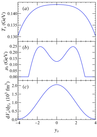
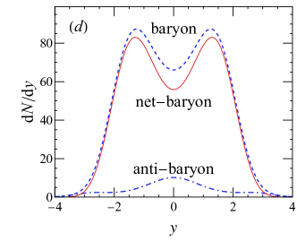
Figure 2: Variation of thermodynamic parameters with source rapidity ($y_{s}$) for the thermal source at $\sqrt{s_{\mathrm{NN}}}=19.6~{}\mathrm{GeV}$: ($a$) temperature ($T_{s}$), ($b$) baryon chemical potential ($\mu_{s}$), and ($c$) volume ($\mathrm{d}{V_{s}}/\mathrm{d}{y_{s}}$). Additionally, ($d$) illustrates the rapidity-dependent yields of baryons (blue dashed), anti-baryons (blue dot-dashed), and net-baryons (red solid).

IV.1 Net-baryon cumulants

This study focuses on investigating the rapidity scan at $\sqrt{s_{\mathrm{NN}}}=19.6~{}\mathrm{GeV}$, a beam energy where various observables exhibit non-monotonic behaviors in beam energy [36]. Extending the investigation to other beam energies is a natural extension, which we reserve for a future more comprehensive investigation. The thermodynamic profiles for rapidity-dependent variables associated with chemical freeze-out are adopted from Ref. [48], displayed in FIG. 2 ($a,\,b,\,c$). The hadron species that carry a singular baryon charge (i.e., $B_{h}=1$) are considered in this study (see a list summarized in Ref. [60]). The resulting rapidity-dependent yields for baryons, anti-baryons, and net-baryons are further illustrated in FIG. 2 ($d$). Employing these rapidity-dependent freeze-out profiles, we investigate the behavior of cumulants by manipulating both the center and width of the rapidity acceptance window. To achieve this, we segment the $y\in[0,3]$ range into smaller bins of equal width, forming rapidity acceptance windows such as $[0,w)$, $[w,2w)$, and so forth up to $[3-w,3]$. To assess the impact of bin width variations, we compare three different widths: $w=0.01$, $0.25$, and $1.00$. Figure 3 exhibits the first to sixth-order net-baryon cumulants normalized by the rapidity bin width ($w$).

We observe a notable trend in FIG. 3: with increasing order of cumulants, their dependence on the bin width ($w$) becomes more pronounced. This heightened sensitivity arises due to the intricate relationship between the cumulants and acceptances ($\alpha_{B}$ and $\alpha_{\bar{B}}$), as shown in Eq. (C) when values for $\left<N_{B}\right>$ and $\left<N_{\bar{B}}\right>$ are fixed. Notably, the $\kappa_{n}^{B}$’s are $n$th-order polynomials of acceptances in Eq. (C), where the magnitudes of acceptances are roughly proportional to the width $w$. Consequently, the non-linear terms of acceptances in $\kappa_{n}^{B}$’s become more significant in coarse rapidity scans, particularly for large bin widths such as $w=0.25$ or $1.00$. Conversely, in the fine rapidity scan ($w=0.01$), the cumulants align closely with those predicted by a Skellam distribution [38, 56] in the case of GCE, which agrees with both mathematical and physical expectations. Mathematically, when the bin width is extremely small, a linear approximation in acceptances for cumulants becomes appropriate. As shown by Eq. (C), this approximation yields $\kappa_{\text{odd}}^{B}\approx\left<N_{B}\right>_{A}-\left<N_{\bar{B}}\right>_{A}$ and $\kappa_{\text{even}}^{B}\approx\left<N_{B}\right>_{A}+\left<N_{\bar{B}}\right>_{A}$, resulting in minimal dependence on $w$ in the case of fine scans. From a thermodynamic standpoint, the system within each rapidity bin can be considered a subsystem, and consequently, with exceedingly small bin widths, these subsystems become less sensitive to the global net-baryon number conservation governing the entire system described by CE. This scenario parallels the conditions where the Skellam distribution becomes an appropriate description for net-baryon fluctuations, portraying baryons and anti-baryons as independently fluctuating, following Poisson distributions. Further discussions on this topic can be found in Appendix D.

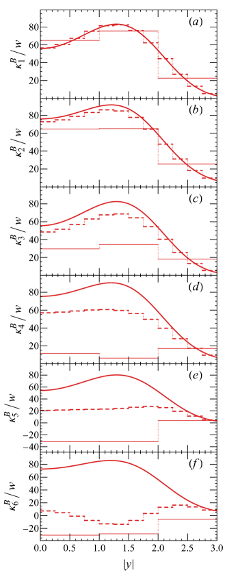
Figure 3: Sequential representation from top to bottom of the first to sixth order scaled cumulants of net baryon fluctuation, normalized by the rapidity bin width ($w$). Each plot illustrates results corresponding to rapidity acceptance windows spanning $[0,w)$, $[w,2w)$, and extending to $[3-w,3]$. Three distinct bin widths are depicted: $w=0.01$ (solid lines), $w=0.25$ (dashed lines), and $w=1.00$ (thin solid lines).

In studies of heavy-ion collisions, various models incorporating a quark-hadron crossover [61, 62] and those excluding it [63, 64] have computed net-proton cumulants. These studies found that the first to fourth-order cumulants show consistent positivity, while the fifth and sixth-order cumulants exhibit a negative sign in scenarios considering a critical transition. In our analysis, where critical fluctuations are absent, we observe intriguing behaviors in $\kappa_{5}^{B}$ and $\kappa_{6}^{B}$ concerning various rapidity bin widths. As depicted in FIG. 3 $\left(e,\,f\right)$, these cumulants maintain positivity with smaller widths and become negative as the widths increase because of the nonlinear terms that are negative in Eq. (C). Consequently, finite acceptances might influence the sign of high-order net-baryon cumulants even without considering critical contributions. We speculate that our findings on net-baryon cumulants could potentially extend to net-proton cumulants, which are measured in experiments, at a qualitative level [65]. Further statistical measures inferred from low-order cumulants are detailed in FIG. 7 in Appendix C.

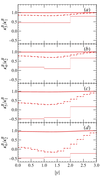
Figure 4: Similar to FIG. 3 but these plots depict the ratios of cumulants for even and odd orders separately: ($a$) $\kappa_{3}^{B}/\kappa_{1}^{B}$, ($b$) $\kappa_{4}^{B}/\kappa_{2}^{B}$, ($c$) $\kappa_{5}^{B}/\kappa_{1}^{B}$ and ($d$) $\kappa_{6}^{B}/\kappa_{2}^{B}$. The three line styles correspond to different acceptance window widths: $w=0.01$ (solid), $w=0.25$ (dashed), and $w=1.00$ (thin solid).

The ratios among these cumulants, $\kappa_{3}^{B}/\kappa_{1}^{B}$, $\kappa_{4}^{B}/\kappa_{2}^{B}$, $\kappa_{5}^{B}/\kappa_{1}^{B}$, and $\kappa_{6}^{B}/\kappa_{2}^{B}$, are depicted in FIG. 4. The figure distinctly illustrates their dependencies on the rapidity bin width $w$. As $w$ diminishes towards zero, these ratios converge toward their GCE limit, approaching unity, consistent with the expected behavior. An intriguing aspect lies in examining the ordering of these cumulants for different bin widths. Lattice QCD predictions indicate a specific ordering of baryon number susceptibilities $\chi_{3}^{B}/\chi_{1}^{B}>\chi_{4}^{B}/\chi_{2}^{B}>\chi_{5}^{B}/\chi_{1}^{B}>\chi_{6}^{B}/\chi_{2}^{B}$ [61], notably absent in ideal GCE statistical thermal model calculations [38, 56, 39]. We explore this ordering in our calculations using obtained cumulants, using the fact that $\chi_{m}^{B}/\chi_{n}^{B}=\kappa_{m}^{B}/\kappa_{n}^{B}$ at a fixed temperature. In FIG. 4, we observe this cascading ordering for $w=0.25$ and $1.00$, yet it’s absent for $w=0.01$. (The vertical axes’ ranges are identical for better comparison across cumulants.) The discrepancy in ordering suggests that changes in bin widths, influencing the impact of the global net-baryon conservation constraint in a CE system, can either induce or disrupt such cascading order of these cumulants. Therefore, it becomes crucial to consider the effect associated with net-baryon conservation via varying bin widths when comparing measurements with lattice QCD results.

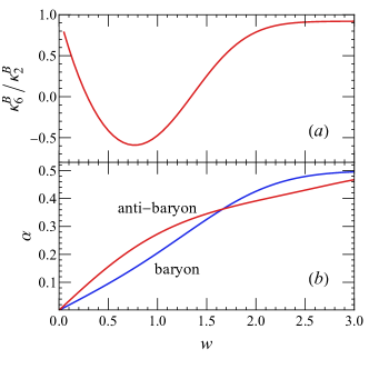
Figure 5: Variation of ($a$) the cumulant ratio $\kappa^{B}_{6}/\kappa^{B}_{2}$ and ($b$) baryon (red) and anti-baryon (blue) acceptances as a function of the changing width of the rapidity window $y\in[0,w]$.

As higher-order cumulants are more sensitive to critical points, we delve deeper into the behavior of the cumulant ratio $\kappa_{6}^{B}/\kappa_{2}^{B}$ and explore how it varies with the changing width $w$ of the rapidity window $y\in[0,w]$. We are specifically examining the positive half of a rapidity window centered at midrapidity $y=0$ (the latter is the region where experimental data are commonly measured). Within this window, the maximum acceptance reaches 0.5 when the rapidity window coverage is sufficiently broad. FIG. 5 illustrates that as the rapidity window widens and thus substantial acceptance coverage is approached, the $\kappa_{6}^{B}/\kappa_{2}^{B}$ ratio reaches a plateau, saturating towards a value near unity. This phenomenon occurs as the acceptances approach 0.5, indicating the inclusion of most particles and antiparticles. Intriguingly, the behavior of $\kappa_{6}^{B}/\kappa_{2}^{B}$ is non-monotonic and changes sign when the rapidity window has $w\in\left[0.5,1.0\right]$, solely due to the increasing bin width and corresponding rising acceptances, despite the absence of any critical behavior considered in our calculation. FIG. 5, together with FIGs. 3 and 4, illustrates the significant impact of finite acceptance on the non-critical yet non-trivial behaviors observed in net-baryon cumulants. Some of these observed behaviors exhibit characteristics resembling non-monotonic trends typically associated with critical effects. Therefore, these results highlight the crucial importance of accounting for finite acceptance, when investigating the high-order net-proton cumulants within a limited rapidity window.

From the perspective of beam energy scan, high-order net-proton cumulants are commonly measured within a finite rapidity window centered around midrapidity to enhance statistical precision, spanning different beam energies. For instance, the STAR collaboration measures net-proton cumulants within the rapidity range $|y|{\,<\,}1$. However, at lower beam energies characterized by smaller beam rapidities, the acceptances of particles are expected to increase within a fixed rapidity coverage when the beam energy decreases. As seen in FIG. 5, the varying acceptances across different beam energies may impact the observed behaviors of high-order cumulants. Therefore, careful consideration is necessary when attempting to discern potential critical phenomena from the non-monotonic behaviors observed in net-proton cumulants at low beam energies or from their deviation from the non-critical statistical thermal baseline [45, 46].

IV.2 Extraction of thermodynamic variables

Having analyzed the rapidity-dependent net-baryon cumulants and their intricate relationship with varying rapidity bin widths, we turn to another pertinent exploration: Extracting the thermodynamic characteristics of a system exhibiting inhomogeneity along the beam axis from net-baryon cumulants obtained within distinct rapidity windows, such as those from experimental measurements. Ideally, the derived effective thermodynamic properties should accurately replicate the given (or measured) net-baryon cumulants. To address this issue, we will leverage the relationship we discussed between Eq. (18) and Eq. (20). The former pertains to the generating function within a particular rapidity window, while the latter describes a singular source with specific temperature and baryon chemical potential. If we identify a singular thermal source capable of producing the same generating function as that within a rapidity window, it can effectively reproduce the corresponding net-baryon cumulants.

Specifically, considering the net-baryon cumulants within a rapidity window of $[y_{c}-w/2,y_{c}+w/2]$, we position a thermal source at $y_{s}{\,=\,}y_{c}$, aligning with the center of the target window. This thermal source, characterized by its temperature $(T_{\mathrm{E}})$, baryon chemical potential $(\mu_{B}^{\mathrm{E}})$, and volume $(V_{\mathrm{E}})$, with the superscript or subscript $\mathrm{E}$ denoting their representation as effective thermodynamic variables of the rapidity window, has the rapidity-differential single-particle partition function outlined in Eq. (7) for a single source. A comparison between equations (18) and (20) reveals that for the generating function of the singular thermal source to match that of the rapidity window, the effective temperature $(T_{\mathrm{E}})$, effective baryon chemical potential $(\mu_{B}^{\mathrm{E}})$, and effective volume $(V_{\mathrm{E}})$ should be adjusted so that the former can replicate the acceptances of both baryons and anti-baryons observed in the latter:

$$\alpha_{B}^{\mathrm{E}}\left(\mu_{B}^{\mathrm{E}},T_{\mathrm{E}},V_{\mathrm{E}}\right)=\alpha_{B}\,,\quad\alpha_{\bar{B}}^{\mathrm{E}}\left(\mu_{B}^{\mathrm{E}},T_{\mathrm{E}},V_{\mathrm{E}}\right)=\alpha_{\bar{B}}\,.$$ (22)

Results depicting the acceptances [$\alpha_{B}$ and $\alpha_{\bar{B}}$ on the right-hand side of Eq. (22)] within various rapidity bins for three distinct bin widths are presented in FIG. 6 ($a$). Indeed, as anticipated, the distributions of baryon and anti-baryon acceptances follow the distributions of their respective yields. Besides, the partition functions should satisfy:

$$z\left(T_{\mathrm{E}},\,V_{\mathrm{E}}\right)=\sqrt{\mathcal{z}\bar{\mathcal{z}}}\,,$$ (23)

where on the left-hand side, the partition function is given by Eq. (21) for a singular source, while the right-hand side, a term from Eq. (18), is a quantity defined for the entire system exhibiting inhomogeneity along the beam axis.

Ideally, to obtain the effective thermodynamic parameters within each rapidity bin, it is necessary to fine-tune the parameters such that they satisfy both Eq. (22) and Eq. (23). However, as evident from FIG. 2 ($a$), the temperature variation along the rapidity axis at $\sqrt{s_{\mathrm{NN}}}=19.6$ GeV is notably small. Given this observation, we will aim to simplify the process by estimating a constant effective temperature across all rapidity bins. To achieve this, we position a singular thermal source at $y_{s}=0$ to represent the entire fireball. We require that the effective temperature $T_{\mathrm{E}}$ and volume $V_{\mathrm{E}}^{\mathrm{tot}}$ of this source have specific values that satisfy Eq. (23). Here, we employ the total volume of the entire fireball, as depicted in FIG. 2 ($c$), to estimate the effective volume value, namely, $V_{\mathrm{E}}^{\mathrm{tot}}=\int_{-\infty}^{+\infty}\mathrm{d}y_{s}\,\mathrm{d}V_{s}/\mathrm{d}y_{s}$. By substituting $V_{\mathrm{E}}^{\mathrm{tot}}$ into Eq. (23), we derive the effective temperature $T_{\mathrm{E}}\approx 144.1$ MeV for $\sqrt{s_{\mathrm{NN}}}=19.6$ GeV. Admittedly, our method of deriving the effective volume relies on information that is unknown from the experimental measurements and thus should be improved in the future. However, this oversight is acceptable as our primary focus lies in extracting the effective chemical potential exhibiting more pronounced variation from the net-baryon cumulants.

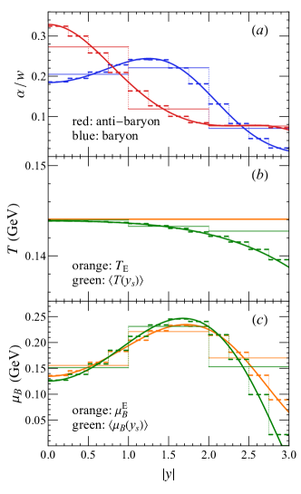
Figure 6: ($a$) Scaled acceptances of baryons (red) and anti-baryons (blue), ($b$) effective $T_{\mathrm{E}}$ (orange) and average $\left<T\left(y_{s}\right)\right>$ (green) temperatures, as well as ($c$) effective $\mu_{B}^{\mathrm{E}}$ (orange) and average $\left<\mu_{B}\left(y_{s}\right)\right>$ (green) baryon chemical potentials. Their variations across three different rapidity bins: $w{\,=\,}0.01$ (solid), $w{\,=\,}0.25$ (dashed), and $w{\,=\,}1.00$ (thin solid lines) are also illustrated.

Now, employing the acquired $T_{\mathrm{E}}\approx 144.1$ MeV as the effective temperature across all rapidity bins [see FIG. 6 ($b$)], our next step involves extracting the effective baryon chemical potential using Eqs. (22). The acceptances of baryons and anti-baryons corresponding to the singular thermal source representing a specific rapidity bin $[y_{c}-w/2,y_{c}+w/2]$ are respectively determined by

$$\begin{gathered}\alpha_{B}^{\mathrm{E}}\left(\mu_{B}^{\mathrm{E}},T_{\mathrm{E}},V_{\mathrm{E}}\right)=\frac{\left<N_{B}^{\mathrm{E}}\right>_{A}}{\left<N_{B}\right>}\,,\\ \alpha_{\bar{B}}^{\mathrm{E}}\left(\mu_{B}^{\mathrm{E}},T_{\mathrm{E}},V_{\mathrm{E}}\right)=\frac{\left<N_{\bar{B}}^{\mathrm{E}}\right>_{A}}{\left<N_{\bar{B}}\right>}\,.\end{gathered}$$ (24)

Within the rapidity window, the numbers of baryons and anti-baryons can be computed respectively using

$$\begin{gathered}\left<N_{B}^{\mathrm{E}}\right>_{A}=\sum_{h}\int_{y_{c}-\frac{w}{2}}^{y_{c}+\frac{w}{2}}\mathrm{e}^{\frac{\mu_{B}^{\mathrm{E}}}{T_{\mathrm{E}}}}z_{h}\left(T_{\mathrm{E}},V_{\mathrm{E}};y-y_{c}\right)\mathrm{d}y\,,\\ \left<N_{\bar{B}}^{\mathrm{E}}\right>_{A}=\sum_{h}\int_{y_{c}-\frac{w}{2}}^{y_{c}+\frac{w}{2}}\mathrm{e}^{-\frac{\mu_{B}^{\mathrm{E}}}{T_{\mathrm{E}}}}z_{h}\left(T_{\mathrm{E}},V_{\mathrm{E}};y-y_{c}\right)\mathrm{d}y\,,\end{gathered}$$ (25)

where $z_{h}$ is the partition function of a hadron species introduced in Eq. (7). In principle, the effective volume in Eq. (25) could also be adjusted individually for each rapidity bin, but our primary focus lies in determining the baryon chemical potential, hence we refrain from explicitly extracting the volume. For this purpose, replicating the ratio of baryon and anti-baryon acceptances within the rapidity window in the singular source is sufficient, i.e.,

$$\frac{\alpha_{B}^{\mathrm{E}}\left(\mu_{B}^{\mathrm{E}},T_{\mathrm{E}},V_{\mathrm{E}}\right)}{\alpha_{\bar{B}}^{\mathrm{E}}\left(\mu_{B}^{\mathrm{E}},T_{\mathrm{E}},V_{\mathrm{E}}\right)}=\frac{\alpha_{B}}{\alpha_{\bar{B}}}\,,$$ (26)

where volume is cancelled out when calculating the ratio. The effective chemical potential can be derived by solving Eq. (26), and the results for three distinct bin widths are presented in FIG. 6 ($c$).

To evaluate the effective thermodynamic variables derived from the rapidity-dependent net-baryon cumulants, we can compare them against the thermodynamic profiles depicted in FIG. 2, which are used for obtaining these cumulants. Given the varying nature of these profiles across rapidity, we shall define the average thermodynamic variables, including the average temperature $\left<T\left(y_{s}\right)\right>$ and baryon chemical potential $\left<\mu_{B}(y_{s})\right>$, based on the smooth profiles within distinct rapidity bins. For a rapidity window $y_{s}\in\left[y_{c}-w/2,y_{c}+w/2\right]$, we calculate these average variables by requiring them to yield identical GCE partition functions and net-baryon values as calculated from the smooth profiles:

$$\begin{split}&2\cosh\left(\frac{\left<\mu_{B}(y_{s})\right>}{\left<T\left(y_{s}\right)\right>}\right)z\left(\left<T\left(y_{s}\right)\right>,\int_{y_{c}-\frac{w}{2}}^{y_{c}+\frac{w}{2}}\frac{\mathrm{d}{V}}{\mathrm{d}{y_{s}}}\mathrm{d}{y_{s}}\right)\\ =\;&\int_{y_{c}-\frac{w}{2}}^{y_{c}+\frac{w}{2}}\mathrm{d}{y_{s}}\int_{-\infty}^{+\infty}\mathrm{d}{y}\sum_{h}\left(\mathcal{z}_{h}^{s}+\bar{\mathcal{z}}_{h}^{s}\right)\,,\\ &2\sinh\left(\frac{\left<\mu_{B}\left(y_{s}\right)\right>}{\left<T\left(y_{s}\right)\right>}\right)z\left(\left<T\left(y_{s}\right)\right>,\int_{y_{c}-\frac{w}{2}}^{y_{c}+\frac{w}{2}}\frac{\mathrm{d}{V}}{\mathrm{d}{y_{s}}}\mathrm{d}{y_{s}}\right)\\ =\;&\int_{y_{c}-\frac{w}{2}}^{y_{c}+\frac{w}{2}}\mathrm{d}{y_{s}}\int_{-\infty}^{+\infty}\mathrm{d}{y}\sum_{h}\left(\mathcal{z}_{h}^{s}-\bar{\mathcal{z}}_{h}^{s}\right)\,.\end{split}$$ (27)

Here, the left-hand side denotes the GCE partition function and the resulting net-baryon number calculated for a singular source, whereas the right-hand side corresponds to the corresponding values derived from the continuous freeze-out profiles presented in FIG. 2. The average variables across distinct rapidity windows for three different rapidity bin widths are illustrated in FIG. 6. These average variables converge toward the continuous freeze-out profiles depicted in FIG. 2 when the bin widths become exceedingly small.

FIG. 6 ($b$) illustrates an intriguing trend that emerges with increasing bin width $w$: the average temperature $\left<T\left(y_{s}\right)\right>$ within a rapidity window appears to approach the highest temperature observed within the same bin. It also shows that the constant effective temperature $T_{\mathrm{E}}$ approximately matches the highest temperature within the continuous freeze-out temperature profile. These trends can be understood by accounting for the influence of total net-baryon conservation across the entire system, as outlined in Eq. (8). Within a rapidity bin governed by the GCE, the fluctuations of baryons and anti-baryons contribute to the free energy of the (sub)system, represented by the fugacity factor $\exp\left(\mu_{B}/T\right)$. In contrast, the CE suppresses these fluctuations, a scenario that becomes more pronounced with larger rapidity bins. In our method of extraction, achieving equivalent thermodynamic properties requires compensating for the energy contributed by fluctuations absent in CE. Therefore, a higher temperature is necessary to align these properties with larger rapidity bins. For a deeper understanding of this concept, interested readers may refer to FIG. 1 in Ref. [52]. FIG. 6 ($c$) demonstrates closely matching values between the derived chemical potential ($\mu_{B}^{\mathrm{E}}$) and the averaged value ($\left<\mu_{B}\left(y_{s}\right)\right>$) across distinct rapidity bins, showcasing small differences partially attributed to the thermal smearing effect. FIG. 6 illustrates a close agreement between the effective thermodynamic variables obtained from the rapidity-dependent net-baryon cumulants and the averaged values derived from the continuous profiles showcased in FIG. 2, which underlines the efficacy of the extraction method.

V Summary and outlook

The upcoming BES-II measurements with improved statistical precision and expanded rapidity-dependent data, will play a crucial role in searching for the critical phenomena, especially through high-order net-proton cumulants across a broad range of beam energies. In this study, we explored the statistical thermal model which integrates rapidity-dependent freeze-out profiles to characterize variances in thermodynamic properties along the beam axis.

We derived analytical expressions for net-baryon cumulants within finite rapidity ranges, maintaining total net-baryon conservation under the canonical ensemble for the entire system. The exploration of rapidity-dependent net-baryon cumulants at $\sqrt{s_{\mathrm{NN}}}=19.6$ GeV underscored the substantial influence of finite acceptance on their behavior with varying rapidity windows. As depicted in figures. 3, 4, and 5, these kinematic acceptances significantly affected high-order cumulant behaviors, unveiling non-trivial trends which can be similar to characteristics associated with critical effects. This observation strongly advocates for considering finite acceptance when interpreting high-order net-proton cumulants measured within confined rapidity windows.

In the context of Beam Energy Scan, where these cumulants are observed within a fixed rapidity range around midrapidity, variations in particle acceptances due to varying beam rapidity across different beam energies are expected to emerge as pivotal factors. Therefore, careful investigation is essential when searching for potential critical phenomena through the energy dependence of net-proton cumulants. Additionally, our study investigated methods to derive effective temperature and baryon chemical potential values, advancing the rapidity scan approach in probing the QCD phase diagram.

Future studies will refine extraction methods for thermodynamic variables, integrating identified hadrons with feed-down effects. Incorporating both critical phenomena (quark-hadron transition, non-Gaussian fluctuations) and non-critical contributions (non-equilibrium corrections, volume fluctuations) will further improve the rapidity scan utilizing Beam Energy Scan measurements and facilitate unraveling phenomena associated with the QCD critical point.

Appendix A Single-particle partition functions table

Table 1 provides a comprehensive summary detailing the symbols and interpretations of various partition functions.

Convention	Eq.	Single-particle partition function of
$z_{h}^{s}$	(6)	$h$ radiated from $s$ in CE
$z_{h}^{s}\left(y\right)$	(7)	$h$ radiated from $s$ distributing on $y$ in CE
$\mathcal{z}_{h}^{s}\left(y-y_{s}\right)$	(8)	baryon $h$ at $y$ radiated from $s$ at $y_{s}$ in GCE
$\bar{\mathcal{z}}_{h}^{s}\left(y-y_{s}\right)$	(8)	anti-baryon $h$ at $y$ radiated from $s$ at $y_{s}$ in GCE
$\mathcal{z}_{A,h}^{s}$	(10)	baryon $h$ in acceptance radiated from $s$ at $y_{s}$ in GCE
$\bar{\mathcal{z}}_{A,h}^{s}$	(10)	anti-baryon $h$ in acceptance radiated from $s$ at $y_{s}$ in GCE
$\mathcal{z}_{R,h}^{s}$	(11)	baryon $h$ outside acceptance radiated from $s$ at $y_{s}$ in GCE
$\bar{\mathcal{z}}_{R,h}^{s}$	(11)	anti-baryon $h$ outside acceptance radiated from $s$ at $y_{s}$ in GCE
$\mathcal{z}_{A}$	(14)	baryons in acceptance in GCE
$\bar{\mathcal{z}}_{A}$	(14)	anti-baryons in acceptance in GCE
$\mathcal{z}_{R}$	(14)	baryons outside acceptance in GCE
$\bar{\mathcal{z}}_{R}$	(14)	anti-baryons outside acceptance in GCE
$\mathcal{z}$	(19)	baryons in full phase space in GCE
$\bar{\mathcal{z}}$	(19)	anti-baryons in full phase space in GCE
$z_{h}$	(21)	$h$ in single-source model in CE
$z$	(21)	single-source model in CE

Table 1: Conventions of single-particle partition functions.

Appendix B On the connection between Eq. (18) and Eq. (20)

As previously mentioned, the variables ${\mathcal{z}}$, $\bar{\mathcal{z}}$, $\alpha_{{B}}$, and $\alpha_{\bar{B}}$ in Eq. (18) pertain to a system characterized by rapidity inhomogeneity. Conversely, the quantities outlined in Eq. (20) are computed for a homogeneous or singular thermal source. To bridge the connection between these two generating functions, we will introduce a few additional approximations.

In CE, the expected values of baryon and anti-baryon numbers for a singular source are determined by [41]

$$\left<N_{B}\right>=z\frac{I_{B-1}\left(2z\right)}{I_{B}\left(2z\right)}\,,\qquad\left<N_{\bar{B}}\right>=z\frac{I_{B+1}\left(2z\right)}{I_{B}\left(2z\right)}\,.$$ (28)

In the high-energy limit, where $\left<N_{B}\right>\approx\left<N_{\bar{B}}\right>\gg B$, the total net-baryon number $B\approx 0$. Utilizing the asymptotic form of $I_{\nu}\left(x\right)$ for $x\gg\left|\nu^{2}-1/4\right|$ [41],

$$\begin{split}\lim_{x\gg\left|\nu^{2}-\frac{1}{4}\right|}I_{\nu}\left(x\right)&=\frac{\mathrm{e}^{x}}{\sqrt{2\pi x}}\left(1-\frac{4\nu^{2}-1}{8x}\cdots\right)\,,\end{split}$$ (29)

we obtain $\left<N_{B}\right>\approx\left<N_{\bar{B}}\right>\approx z$. In low-energy collisions, utilizing the asymptotic form of $I_{\nu}\left(z\right)$ at $\nu\rightarrow\infty$ [66],

$$\lim_{\nu\rightarrow\infty}I_{\nu}\left(x\right)=\frac{1}{\sqrt{2\pi\nu}}\left(\frac{\mathrm{e}x}{2\nu}\right)^{\nu},\quad x\neq 0\,,$$ (30)

we obtain $\left<N_{B}\right>\approx B$ and $\left<N_{\bar{B}}\right>\approx z^{2}/B$ because $B\gg 1$. In both scenarios, we can consistently observe that $z\approx\sqrt{\left<N_{B}\right>\left<N_{\bar{B}}\right>}$ for a singular thermal source within CE.

In the main text, we have shown that when solely considering baryons carrying a single baryon charge and excluding light nuclei with $B_{h}>1$, $\mathcal{z}$ and $\bar{\mathcal{z}}$ yield the expected values of baryons $\left<N_{B}\right>$ and anti-baryons $\left<N_{\bar{B}}\right>$ in the full phase space. Consequently, in a system characterized by rapidity inhomogeneity, it follows that $\sqrt{\mathcal{z}\bar{\mathcal{z}}}\approx\sqrt{\left<N_{B}\right>\left<N_{\bar{B}}\right>}$. Thus, it can be seen that both $\sqrt{\mathcal{z}\bar{\mathcal{z}}}\approx\sqrt{\left<N_{B}\right>\left<N_{\bar{B}}\right>}$ in Eq. (18) for a system characterized by rapidity inhomogeneity and $z\approx\sqrt{\left<N_{B}\right>\left<N_{\bar{B}}\right>}$ in Eq. (20) for a singular source reflect the characteristics of the CE.

Appendix C Expressions of the first to sixth order cumulants and statistical measures

For clarity and coherence within this study, we present the analytical expressions of cumulants up to the sixth order in this section. It’s worth noting that this formalism is introduced and developed in Ref. [41]. With the following notations

$$\kappa_{1}^{\pm} =\frac{1}{2}\left(\alpha_{B}\pm\alpha_{\bar{B}}\right)\,,$$

$$\kappa_{2}^{\pm} =\frac{1}{2}\left[\alpha_{B}\left(1-\alpha_{B}\right)\mp\left(\alpha_{B}\leftrightarrow\alpha_{\bar{B}}\right)\right]\,,$$

$$\kappa_{3}^{\pm} =\frac{1}{2}\left[\alpha_{B}\left(1-\alpha_{B}\right)\left(1-2\alpha_{B}\right)\pm\left(\alpha_{B}\leftrightarrow\alpha_{\bar{B}}\right)\right]\,,$$

$$\kappa_{4}^{\pm} =\frac{1}{2}\left[\alpha_{B}\left(1-\alpha_{B}\right)\left(1-6\alpha_{B}+6\alpha_{B}^{2}\right)\mp\left(\alpha_{B}\leftrightarrow\alpha_{\bar{B}}\right)\right]\,,$$ (31)

$$\kappa_{5}^{\pm} =\frac{1}{2}\,\Big{[}\alpha_{B}\left(1-\alpha_{B}\right)\left(1-2\alpha_{B}\right)\left(1-12\alpha_{B}+12\alpha_{B}^{2}\right)$$

$$\qquad\pm\left(\alpha_{B}\leftrightarrow\alpha_{\bar{B}}\right)\Big{]}\,,$$

$$\kappa_{6}^{\pm} =\frac{1}{2}\,\Big{[}\alpha_{B}\left(1-\alpha_{B}\right)\left(1-30\alpha_{B}+150\alpha_{B}^{2}-240\alpha_{B}^{3}+120\alpha_{B}^{4}\right)$$

$$\qquad\mp\left(\alpha_{B}\leftrightarrow\alpha_{\bar{B}}\right)\Big{]}\,,$$

the first to sixth-order cumulants can be expressed as

$$\kappa_{1}^{B} =B\kappa_{1}^{+}+S\kappa_{1}^{-}\,,$$

$$\kappa_{2}^{B} =B\kappa_{2}^{+}+S\kappa_{2}^{-}\,,$$

$$\kappa_{3}^{B} =B\kappa_{3}^{+}+S\kappa_{3}^{-}+8P\left(\kappa_{1}^{-}\right)^{3}\,,$$ (32)

$$\kappa_{4}^{B} =B\kappa_{4}^{+}+S\kappa_{4}^{-}+48P\left(\kappa_{1}^{-}\right)^{2}\kappa_{2}^{-}-16P\left(S-1\right)\left(\kappa_{1}^{-}\right)^{4}\,,$$

$$\kappa_{5}^{B} =B\kappa_{5}^{+}+S\kappa_{5}^{-}+40P\left[3\kappa_{1}^{-}\left(\kappa_{2}^{-}\right)^{2}+2\left(\kappa_{1}^{-}\right)^{2}\kappa_{3}^{-}\right]$$ (33)

$$\quad-160P\left(S-1\right)\left(\kappa_{1}^{-}\right)^{3}\kappa_{2}^{-}+32P\left(S^{2}-S+1\right)\,,$$

$$\kappa_{6}^{B} =B\kappa_{6}^{+}+S\kappa_{6}^{-}+120P\left[4\kappa_{1}^{-}\kappa_{2}^{-}\kappa_{3}^{-}+\left(\kappa_{1}^{-}\right)^{2}\kappa_{4}^{-}+\left(\kappa_{2}^{-}\right)^{3}\right]$$

$$\quad-80P\left(S-1\right)\left[4\left(\kappa_{1}^{-}\right)^{3}\kappa_{3}^{-}+9\left(\kappa_{1}^{-}\right)^{2}\left(\kappa_{2}^{-}\right)^{2}\right]$$

$$\quad+480P\left(S^{2}-S+1\right)\left(\kappa_{1}^{-}\right)^{4}\kappa_{2}^{-}$$

$$\quad-64P\left[\left(S^{3}-S^{2}+S-1\right)+6P\right]\left(\kappa_{1}^{-}\right)^{6}\,.$$

Here we have employed the same abbreviations introduced in Ref. [41], summarized below:

$$S=\left<N_{B}\right>+\left<N_{\bar{B}}\right>\,,\qquad P=\left<N_{B}\right>\left<N_{\bar{B}}\right>\,.$$ (34)

Some abbreviations may yield different results compared to those shown in Ref. [41]. This discrepancy arises due to the condition $\mathcal{z}\bar{\mathcal{z}}\approx\left<N_{B}\right>\left<N_{\bar{B}}\right>$ within our framework, resulting in $Q=\mathcal{z}\bar{\mathcal{z}}-P\approx 0$ and $W=QS-P\approx-P$.

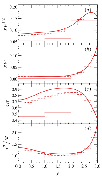
Figure 7: Same as FIGs. 3 and 4 but for (scaled) statistical measures: ($a$) $sw^{1/2}$, ($b$) $\kappa w$, ($c$) $s\sigma$ and ($b$) $\sigma^{2}/M$. Three different rapidity bins are selected: $w=0.01$ (solid), $w=0.25$ (dashed), and $w=1.00$ (thin solid).

These cumulants allow for the calculation of statistical measures such as mean ($M$), variance ($\sigma^{2}$), skewness ($s$), and kurtosis ($\kappa$), which can be expressed as

$$M=\kappa_{1}^{B}\,,\quad\sigma^{2}=\kappa_{2}^{B}\,,\quad s=\frac{\kappa_{3}^{B}}{\left(\kappa_{2}^{B}\right)^{3/2}}\,,\quad\kappa=\frac{\kappa_{4}^{B}}{\left(\kappa_{2}^{B}\right)^{2}}\,.$$ (35)

Moreover, the product of these measures can be expressed in terms of the ratios of cumulants, as demonstrated below

$$\kappa\sigma^{2}=\frac{\kappa_{4}^{B}}{\kappa_{2}^{B}}\,,\quad s\sigma=\frac{\kappa_{3}^{B}}{\kappa_{2}^{B}}\,,\quad\frac{\sigma^{2}}{M}=\frac{\kappa_{2}^{B}}{\kappa_{1}^{B}}\,.$$ (36)

Figures 3($a,\,b$) and 4($b$) present $M/w$, $\sigma^{2}/w$, and $\kappa\sigma^{2}$, respectively. The other scaled statistical measures are displayed in Figure 7.

Appendix D Cumulants of fine scan and GCE (Skellam distribution)

In the main text, we discussed that the system within the entire phase space is characterized by the CE since the total net-baryon number is conserved. However, experimental measurements are confined to finite rapidity windows, and baryons and anti-baryons are subject to fluctuations. As the acceptance window decreases, the constraint from the baryon conservation weakens, allowing for greater independence in fluctuations of both baryons and anti-baryons around their expected values [67, 52]. In this Appendix, we demonstrate the convergence of CE cumulants towards those derived from the Skellam distribution for the GCE when the rapidity window is sufficiently small.

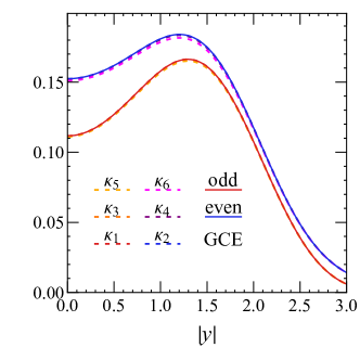
Figure 8: Comparison of the first to sixth order cumulants obtained from a fine rapidity bin with $w=0.002$ (dashed) against the cumulants derived from the Skellam distribution for the GCE (solid), as given in Eq. (38).

Besides deriving cumulants from generating functions, an alternative approach involves calculating them using susceptibilities denoted as $\chi_{n}^{B}$: $\kappa_{n}^{B}=VT^{3}\chi_{n}^{B}$. These susceptibilities are readily obtained from the thermodynamic pressure $P$ through the relationship $\chi_{n}^{B}=T^{n-4}\partial^{n}P/\partial\mu_{B}^{n}$. The thermodynamic pressure within the GCE of the statistical thermal model is

$$P^{\mathrm{GCE}}\left(T,V,\mu_{B}\right)=2\frac{T}{V}\cosh\left(\frac{\mu_{B}}{T}\right)z\left(T,V\right)\,,$$ (37)

where we have adopted $B_{h}=1$ and taken the Maxwell–Boltzmann approximation. As a result, the net-baryon cumulants of both even and odd orders can be expressed as follows:

$$\begin{gathered}\kappa_{\mathrm{odd}}^{\mathrm{GCE}}=2\sinh\left(\frac{\mu_{B}}{T}\right)z\left(T,V\right)=\left<N_{B}\right>-\left<N_{\bar{B}}\right>\,,\\ \kappa_{\mathrm{even}}^{\mathrm{GCE}}=2\cosh\left(\frac{\mu_{B}}{T}\right)z\left(T,V\right)=\left<N_{B}\right>+\left<N_{\bar{B}}\right>\,.\end{gathered}$$ (38)

From this, we can observe that $\kappa_{\mathrm{odd}}^{\mathrm{GCE}}/\kappa_{\mathrm{odd}}^{\mathrm{GCE}}=\kappa_{\mathrm{even}}^{\mathrm{GCE}}/\kappa_{\mathrm{even}}^{\mathrm{GCE}}=1$ and $\kappa_{\mathrm{odd}}^{\mathrm{GCE}}/\kappa_{\mathrm{even}}^{\mathrm{GCE}}=\tanh\left(\mu_{B}/T\right)$, which are also the results of the Skellam distribution [68]. To demonstrate the convergence of net-baryon cumulants, when the rapidity window is small, toward the outcomes predicted by the Skellam distribution (i.e., the results of the GCE), we present a comparative analysis in FIG. (8). The figure effectively illustrates the consistency between the calculated first to sixth-order cumulants using the method in Sec. III for a rapidity bin of $w=0.002$ and those computed using Eq. (38) for the GCE.

References

- An et al. [2022] X. An et al., The BEST framework for the search for the QCD critical point and the chiral magnetic effect, Nucl. Phys. A 1017, 122343 (2022), arXiv:2108.13867 [nucl-th] .
- Aoki et al. [2006] Y. Aoki, G. Endrodi, Z. Fodor, S. D. Katz, and K. K. Szabo, The Order of the quantum chromodynamics transition predicted by the standard model of particle physics, Nature 443, 675 (2006), arXiv:hep-lat/0611014 .
- Abdallah et al. [2021a] M. Abdallah et al. (STAR), Measurement of the Sixth-Order Cumulant of Net-Proton Multiplicity Distributions in Au+Au Collisions at 27, 54.4, and 200 GeV at RHIC, Phys. Rev. Lett. 127, 262301 (2021a), arXiv:2105.14698 [nucl-ex] .
- Bowman and Kapusta [2009] E. S. Bowman and J. I. Kapusta, Critical Points in the Linear Sigma Model with Quarks, Phys. Rev. C 79, 015202 (2009), arXiv:0810.0042 [nucl-th] .
- Ejiri [2008] S. Ejiri, Canonical partition function and finite density phase transition in lattice QCD, Phys. Rev. D 78, 074507 (2008), arXiv:0804.3227 [hep-lat] .
- Barbour et al. [1998] I. M. Barbour, S. E. Morrison, E. G. Klepfish, J. B. Kogut, and M.-P. Lombardo, Results on finite density QCD, Nucl. Phys. B Proc. Suppl. 60, 220 (1998), arXiv:hep-lat/9705042 .
- Aboona et al. [2023] B. Aboona et al. (STAR), Beam Energy Dependence of Fifth and Sixth-Order Net-proton Number Fluctuations in Au+Au Collisions at RHIC, Phys. Rev. Lett. 130, 082301 (2023), arXiv:2207.09837 [nucl-ex] .
- Stephanov et al. [1999] M. A. Stephanov, K. Rajagopal, and E. V. Shuryak, Event-by-event fluctuations in heavy ion collisions and the QCD critical point, Phys. Rev. D 60, 114028 (1999), arXiv:hep-ph/9903292 .
- Stephanov [2009] M. A. Stephanov, Non-Gaussian fluctuations near the QCD critical point, Phys. Rev. Lett. 102, 032301 (2009), arXiv:0809.3450 [hep-ph] .
- Stephanov [2011] M. A. Stephanov, On the sign of kurtosis near the QCD critical point, Phys. Rev. Lett. 107, 052301 (2011), arXiv:1104.1627 [hep-ph] .
- Asakawa et al. [2009] M. Asakawa, S. Ejiri, and M. Kitazawa, Third moments of conserved charges as probes of QCD phase structure, Phys. Rev. Lett. 103, 262301 (2009), arXiv:0904.2089 [nucl-th] .
- Braun-Munzinger and Stachel [2007] P. Braun-Munzinger and J. Stachel, The quest for the quark-gluon plasma, Nature 448, 302 (2007).
- Begun et al. [2018] V. Begun, D. Kikoła, V. Vovchenko, and D. Wielanek, Estimation of the freeze-out parameters reachable in a fixed-target experiment at the CERN Large Hadron Collider, Phys. Rev. C 98, 034905 (2018), arXiv:1806.01303 [nucl-th] .
- Brewer et al. [2018] J. Brewer, S. Mukherjee, K. Rajagopal, and Y. Yin, Searching for the QCD critical point via the rapidity dependence of cumulants, Phys. Rev. C 98, 061901 (2018), arXiv:1804.10215 [hep-ph] .
- Karpenko [2019] I. Karpenko, Rapidity scan in heavy ion collisions at GeV using a viscous hydro cascade model, Acta Phys. Polon. B 50, 141 (2019), arXiv:1805.11998 [nucl-th] .
- Du et al. [2021] L. Du, X. An, and U. Heinz, Baryon transport and the QCD critical point, Phys. Rev. C 104, 064904 (2021), arXiv:2107.02302 [hep-ph] .
- Du et al. [2022] L. Du, X. An, and U. Heinz, Baryon diffusion near the QCD critical point, PoS CPOD2021, 024 (2022), arXiv:2109.06918 [nucl-th] .
- [18] Y. Yin, The QCD critical point hunt: emergent new ideas and new dynamics, arXiv:1811.06519 [nucl-th] .
- Karsch et al. [2003a] F. Karsch, K. Redlich, and A. Tawfik, Thermodynamics at nonzero baryon number density: A Comparison of lattice and hadron resonance gas model calculations, Phys. Lett. B 571, 67 (2003a), arXiv:hep-ph/0306208 .
- Karsch et al. [2003b] F. Karsch, K. Redlich, and A. Tawfik, Hadron resonance mass spectrum and lattice QCD thermodynamics, Eur. Phys. J. C 29, 549 (2003b), arXiv:hep-ph/0303108 .
- Allton et al. [2005] C. R. Allton, M. Doring, S. Ejiri, S. J. Hands, O. Kaczmarek, F. Karsch, E. Laermann, and K. Redlich, Thermodynamics of two flavor QCD to sixth order in quark chemical potential, Phys. Rev. D 71, 054508 (2005), arXiv:hep-lat/0501030 .
- Huovinen and Petreczky [2010] P. Huovinen and P. Petreczky, QCD Equation of State and Hadron Resonance Gas, Nucl. Phys. A 837, 26 (2010), arXiv:0912.2541 [hep-ph] .
- Majumder and Muller [2010] A. Majumder and B. Muller, Hadron Mass Spectrum from Lattice QCD, Phys. Rev. Lett. 105, 252002 (2010), arXiv:1008.1747 [hep-ph] .
- Ratti et al. [2011] C. Ratti, S. Borsanyi, Z. Fodor, C. Hoelbling, S. D. Katz, S. Krieg, and K. K. Szabo (Wuppertal-Budapest), Recent results on QCD thermodynamics: lattice QCD versus Hadron Resonance Gas model, Nucl. Phys. A 855, 253 (2011), arXiv:1012.5215 [hep-lat] .
- Vovchenko and Stoecker [2019] V. Vovchenko and H. Stoecker, Thermal-FIST: A package for heavy-ion collisions and hadronic equation of state, Comput. Phys. Commun. 244, 295 (2019), arXiv:1901.05249 [nucl-th] .
- Becattini et al. [2004] F. Becattini, M. Gazdzicki, A. Keranen, J. Manninen, and R. Stock, Chemical equilibrium in nucleus nucleus collisions at relativistic energies, Phys. Rev. C 69, 024905 (2004), arXiv:hep-ph/0310049 .
- Tawfik [2005] A. Tawfik, QCD phase diagram: A Comparison of lattice and hadron resonance gas model calculations, Phys. Rev. D 71, 054502 (2005), arXiv:hep-ph/0412336 .
- Cleymans et al. [2006] J. Cleymans, H. Oeschler, K. Redlich, and S. Wheaton, Comparison of chemical freeze-out criteria in heavy-ion collisions, Phys. Rev. C 73, 034905 (2006), arXiv:hep-ph/0511094 .
- Andronic et al. [2009] A. Andronic, P. Braun-Munzinger, and J. Stachel, Thermal hadron production in relativistic nuclear collisions: The Hadron mass spectrum, the horn, and the QCD phase transition, Phys. Lett. B 673, 142 (2009), [Erratum: Phys.Lett.B 678, 516 (2009)], arXiv:0812.1186 [nucl-th] .
- Andronic et al. [2018] A. Andronic, P. Braun-Munzinger, K. Redlich, and J. Stachel, Decoding the phase structure of QCD via particle production at high energy, Nature 561, 321 (2018), arXiv:1710.09425 [nucl-th] .
- Du et al. [2023] L. Du, C. Shen, S. Jeon, and C. Gale, Probing initial baryon stopping and equation of state with rapidity-dependent directed flow of identified particles, Phys. Rev. C 108, L041901 (2023), arXiv:2211.16408 [nucl-th] .
- Wheaton and Cleymans [2009] S. Wheaton and J. Cleymans, THERMUS: A Thermal model package for ROOT, Comput. Phys. Commun. 180, 84 (2009), arXiv:hep-ph/0407174 .
- Ejiri et al. [2006] S. Ejiri, F. Karsch, and K. Redlich, Hadronic fluctuations at the QCD phase transition, Phys. Lett. B 633, 275 (2006), arXiv:hep-ph/0509051 .
- Braun-Munzinger et al. [2004] P. Braun-Munzinger, K. Redlich, and J. Stachel, Particle production in heavy ion collisions, in Quark-gluon Plasma 3, edited by R. C. Hwa and X.-N. Wang (2004) pp. 491–599, arXiv:nucl-th/0304013 .
- Tawfik [2014] A. N. Tawfik, Equilibrium statistical-thermal models in high-energy physics, Int. J. Mod. Phys. A 29, 1430021 (2014), arXiv:1410.0372 [hep-ph] .
- Adamczyk et al. [2017] L. Adamczyk et al. (STAR), Bulk Properties of the Medium Produced in Relativistic Heavy-Ion Collisions from the Beam Energy Scan Program, Phys. Rev. C 96, 044904 (2017), arXiv:1701.07065 [nucl-ex] .
- Karsch and Redlich [2011] F. Karsch and K. Redlich, Probing freeze-out conditions in heavy ion collisions with moments of charge fluctuations, Phys. Lett. B 695, 136 (2011), arXiv:1007.2581 [hep-ph] .
- Braun-Munzinger et al. [2011] P. Braun-Munzinger, B. Friman, F. Karsch, K. Redlich, and V. Skokov, Net-proton probability distribution in heavy ion collisions, Phys. Rev. C 84, 064911 (2011), arXiv:1107.4267 [hep-ph] .
- Borsanyi et al. [2018] S. Borsanyi, Z. Fodor, J. N. Guenther, S. K. Katz, K. K. Szabo, A. Pasztor, I. Portillo, and C. Ratti, Higher order fluctuations and correlations of conserved charges from lattice QCD, JHEP 10, 205, arXiv:1805.04445 [hep-lat] .
- Karsch [2017] F. Karsch, Lattice QCD results on cumulant ratios at freeze-out, J. Phys. Conf. Ser. 779, 012015 (2017), arXiv:1611.01973 [hep-lat] .
- Braun-Munzinger et al. [2021] P. Braun-Munzinger, B. Friman, K. Redlich, A. Rustamov, and J. Stachel, Relativistic nuclear collisions: Establishing a non-critical baseline for fluctuation measurements, Nucl. Phys. A 1008, 122141 (2021), arXiv:2007.02463 [nucl-th] .
- Vovchenko and Koch [2021] V. Vovchenko and V. Koch, Particlization of an interacting hadron resonance gas with global conservation laws for event-by-event fluctuations in heavy-ion collisions, Phys. Rev. C 103, 044903 (2021), arXiv:2012.09954 [hep-ph] .
- Vovchenko et al. [2022] V. Vovchenko, V. Koch, and C. Shen, Proton number cumulants and correlation functions in Au-Au collisions at 7.7–200 GeV from hydrodynamics, Phys. Rev. C 105, 014904 (2022), arXiv:2107.00163 [hep-ph] .
- Vovchenko [2022] V. Vovchenko, Correcting event-by-event fluctuations in heavy-ion collisions for exact global conservation laws with the generalized subensemble acceptance method, Phys. Rev. C 105, 014903 (2022), arXiv:2106.13775 [hep-ph] .
- Adam et al. [2021] J. Adam et al. (STAR), Nonmonotonic Energy Dependence of Net-Proton Number Fluctuations, Phys. Rev. Lett. 126, 092301 (2021), arXiv:2001.02852 [nucl-ex] .
- Abdallah et al. [2021b] M. Abdallah et al. (STAR), Cumulants and correlation functions of net-proton, proton, and antiproton multiplicity distributions in Au+Au collisions at energies available at the BNL Relativistic Heavy Ion Collider, Phys. Rev. C 104, 024902 (2021b), arXiv:2101.12413 [nucl-ex] .
- Braun-Munzinger et al. [1999] P. Braun-Munzinger, I. Heppe, and J. Stachel, Chemical equilibration in Pb + Pb collisions at the SPS, Phys. Lett. B 465, 15 (1999), arXiv:nucl-th/9903010 .
- [48] L. Du, H. Gao, S. Jeon, and C. Gale, Rapidity scan with multistage hydrodynamic and statistical thermal models, arXiv:2302.13852 [nucl-th] .
- [49] H. Gao, L. Du, S. Jeon, and C. Gale, Exploring the freeze-out hypersurface with a rapidity-dependent thermal model, in preparation.
- Luo and Xu [2017] X. Luo and N. Xu, Search for the QCD Critical Point with Fluctuations of Conserved Quantities in Relativistic Heavy-Ion Collisions at RHIC : An Overview, Nucl. Sci. Tech. 28, 112 (2017), arXiv:1701.02105 [nucl-ex] .
- Kardar [2007] M. Kardar, Statistical Physics of Particles (Cambridge University Press, 2007).
- Vovchenko et al. [2020] V. Vovchenko, O. Savchuk, R. V. Poberezhnyuk, M. I. Gorenstein, and V. Koch, Connecting fluctuation measurements in heavy-ion collisions with the grand-canonical susceptibilities, Phys. Lett. B 811, 135868 (2020), arXiv:2003.13905 [hep-ph] .
- Cleymans and Koch [1991] J. Cleymans and P. Koch, Multiplicity distribution of strange particles in heavy ion collisions, Z. Phys. C 52, 137 (1991).
- Ko et al. [2001] C. M. Ko, V. Koch, Z.-w. Lin, K. Redlich, M. A. Stephanov, and X.-N. Wang, Kinetic equation with exact charge conservation, Phys. Rev. Lett. 86, 5438 (2001), arXiv:nucl-th/0010004 .
- Cleymans et al. [2005] J. Cleymans, K. Redlich, and L. Turko, Probability distributions in statistical ensembles with conserved charges, Phys. Rev. C 71, 047902 (2005), arXiv:hep-th/0412262 .
- Braun-Munzinger et al. [2012] P. Braun-Munzinger, B. Friman, F. Karsch, K. Redlich, and V. Skokov, Net-charge probability distributions in heavy ion collisions at chemical freeze-out, Nucl. Phys. A 880, 48 (2012), arXiv:1111.5063 [hep-ph] .
- Pathria [2011] R. Pathria, Statistical Mechanics, International series of monographs in natural philosophy (Elsevier Science & Technology Books, 2011).
- Bateman [1953] H. Bateman, Higher transcendental functions [volumes i-iii], Vol. 1 (McGRAW-HILL book company, 1953).
- Bzdak et al. [2013] A. Bzdak, V. Koch, and V. Skokov, Baryon number conservation and the cumulants of the net proton distribution, Phys. Rev. C 87, 014901 (2013), arXiv:1203.4529 [hep-ph] .
- [60] https://github.com/vlvovch/Thermal-FIST/blob/master/input/list/PDG2020/list-all.dat.
- Bazavov et al. [2020] A. Bazavov et al., Skewness, kurtosis, and the fifth and sixth order cumulants of net baryon-number distributions from lattice QCD confront high-statistics STAR data, Phys. Rev. D 101, 074502 (2020), arXiv:2001.08530 [hep-lat] .
- Fu et al. [2021] W.-j. Fu, X. Luo, J. M. Pawlowski, F. Rennecke, R. Wen, and S. Yin, Hyper-order baryon number fluctuations at finite temperature and density, Phys. Rev. D 104, 094047 (2021), arXiv:2101.06035 [hep-ph] .
- Bleicher et al. [1999] M. Bleicher et al., Relativistic hadron hadron collisions in the ultrarelativistic quantum molecular dynamics model, J. Phys. G 25, 1859 (1999), arXiv:hep-ph/9909407 .
- Garg et al. [2013] P. Garg, D. K. Mishra, P. K. Netrakanti, B. Mohanty, A. K. Mohanty, B. K. Singh, and N. Xu, Conserved number fluctuations in a hadron resonance gas model, Phys. Lett. B 726, 691 (2013), arXiv:1304.7133 [nucl-ex] .
- Kitazawa and Asakawa [2012] M. Kitazawa and M. Asakawa, Revealing baryon number fluctuations from proton number fluctuations in relativistic heavy ion collisions, Phys. Rev. C 85, 021901 (2012), arXiv:1107.2755 [nucl-th] .
- Olver et al. [2010] F. Olver, D. Lozier, R. Boisvert, and C. Clark, NIST handbook of mathematical functions hardback and CD-ROM (Cambridge University Press, New York, NY, 2010).
- Koch [2010] V. Koch, Hadronic Fluctuations and Correlations, in Relativistic Heavy Ion Physics, edited by R. Stock (2010) pp. 626–652, arXiv:0810.2520 [nucl-th] .
- Skellam [1946] J. G. Skellam, The frequency distribution of the difference between two poisson variates belonging to different populations, Journal of the Royal Statistical Society Series A: Statistics in Society 109, 296 (1946).