Dynamic System Stability Verification Using Numerical Simulator

Abstract

There are recent shifts in demand for design controllers from simplified to complex model-based. Although simplification approaches are successful in many areas of engineering control systems, high-fidelity simulation-based control design, for example, reinforcement learning, has been rising in robotics areas. On the other hand, the lack of assurances about the stability and robustness of simulation-based control design restricts its applications to safety-critical systems. We develop computational methods to verify the stability and robustness of safety-critical systems. By extending the inverse Lyapunov theorem, we present a practical method to compute the constants required to check the exponential stability conditions of dynamic systems implemented in a numerical simulator. It is shown that the norm-bound of the propagated states is a function of the numerical integration steps, where the numerical simulator may include discontinuous jumps of states. The energy bounds for the transition states are obtained based on the exponential stability assumption of the inverse Lyapunov theorem. Finally, a finite sampling algorithm provides the deterministic stability guarantee for the continuous state space.

I Introduction

Most control design approaches rely on simplified dynamic model descriptions for complex real-world systems. These simplification approaches have been very successful in many engineering systems over the past few decades [1, 2, 3, 4]. However, all control system designs must undergo costly, laborious, and tedious system verification procedures through computational [5] or experimental methods [6, 7]. While there are several immediate challenges in implementing accurate and computationally efficient numerical simulators, it is a common practice to use high-fidelity simulators to verify the performance and robustness of controllers for many engineering systems. In control system design projects, frequently high-fidelity dynamic simulators are available. For example, combining the rotor and wing models for a compound aircraft simulator is presented in [8]. A detailed quad-copter vehicle simulator for abnormal simulations including the full rigid-body dynamics, the propulsion model, the aerodynamics model and the low-level controller has been shown in [9]. Design procedures for implementing a simulator model of an electric motor producing the same responses as the real motor is demonstrated in [10].

Meanwhile, several simulation-based control design approaches have been on the rise recently [11, 12]. The rise of reinforcement learning to solve challenging control problems is particularly noticeable in robotics. The contact dynamics of robot manipulators are difficult to take into account explicitly in the control design steps [13]. The nature of simulation-based control design approaches of reinforcement learning makes it the ideal tool for the control design. On the other hand, the lack of assurances about the stability and robustness of simulation-based control systems makes it challenging to deploy the designs in safety-critical systems such as aircraft, spacecraft and rockets.

In the following sections, we derive the norm bound of states propagated by numerical simulators. The exact calculation of the norm bounds is critical for applying the converse Lyapunov theorem in the stability verification. Based on the norm condition with the exponential stability assumption, a stability assurance algorithm using a finite number of simulations providing the deterministic stability assurance is presented. Finally, the conclusions and future works are discussed.

II Norm-bound of simulator propagated states

Consider the nonlinear system given by [14]

$$\dot{\bf x} ={\bf f}(t,{\bf x})$$ (1)

where ${\bf x}$ is a real-valued $n$-dimensional vector belong to ${\mathbb{R}}^{n}$, which is the $n$-dimensional real space, $\dot{\bf x}=d(\cdot)/dt$ is the derivative of ${\bf x}$ with respect to the time, $t$, and ${\bf f}(t,{\bf x})$ is a continuously differentiable nonlinear function with respect to ${\bf x}$ in ${\mathbb{D}}=\{{\bf x}|\|{\bf x}\|<r\}$ for $r>0$. ${\bf f}(t,{\bf x})$ would include a feedback control system and $\partial{\bf f}/\partial{\bf x}$ is bounded on ${\mathbb{D}}$ implying that $\|{\bf f}(t,{\bf x})\|$ is bounded. In addition, for the uniqueness of the solution, the Lipschitz condition must be satisfied: $\|{\bf f}(t,{\bf x})-{\bf f}(t,{\bf y})\|\leq L\|{\bf x}-{\bf y}\|$ for any ${\bf x}$ and ${\bf y}$ in ${\mathbb{D}}$ and $L>0$. The continuous differentiability and Lipschitz continuity requirements are restrictive for engineering systems to satisfy without introducing tight bounds on the operational conditions.

Instead of the differential equation form of a nonlinear system, (1), consider the following integral-type nonlinear systems

$${\bf x}(t)={\bf x}(t_{0})+\int_{\tau=t_{0}}^{\tau=t}{\bf f}[t,{\bf x}(\tau)]d\tau$$ (2)

where ${\bf f}(t,{\bf x})$ is Lebesgue integrable, which allows discontinuous jumps in the finite number of isolated instances, $t$. This is called the Carathéodory solution [15]. By the definition of (2), the states are automatically continuous and continuously differentiable for almost all $t$. The Lipschitz condition is again required to be satisfied. This is a less restrictive description of nonlinear systems than (1), but it still does not allow discontinuous jumps of ${\bf f}(t,{\bf x})$ in ${\bf x}$.

From now on, we consider the systems without the explicit dependence on time such that (2) becomes

$${\bf x}(t)={\bf x}(t_{0})+\int_{\tau=t_{0}}^{\tau=t}{\bf f}[{\bf x}(\tau)]d\tau$$ (3)

where the continuity of ${\bf f}[{\bf x}(t)]$ in ${\bf x}(t)$ is to be relaxed later. The numerical implementation of (3) is

$${\bf x}(t+\Delta t) =\Phi[t+\Delta t,t,{\bf x}(t)]$$

$$={\bf x}(t)+\int^{\tau=t+\Delta t}_{\tau=t}{\bf f}[{\bf x}(\tau)]d\tau$$ (4)

where $\Phi(t_{1},t_{0},{\bf x}_{0})$ is the state transition function from $t_{0}$ to $t_{1}$ starting at the initial state, ${\bf x}_{0}$ at $t_{0}$ and the integral in the right-hand side is implemented by a numerical method such as the Euler method, i.e.,

$${\boldsymbol{\Phi}}_{\text{Euler}}[t+\Delta t,t,{\bf x}(t)]={\bf x}(t)+{\bf f}[{\bf x}(t)]\Delta t$$ (5)

or the Runge-Kutta method, i.e.,

$${\boldsymbol{\Phi}}_{\text{RK}}[t+\Delta t,t,{\bf x}(t)] ={\bf x}(t)$$

$$+\dfrac{\Delta t}{6}\left({\bf k}_{1}+2{\bf k}_{2}+2{\bf k}_{3}+{\bf k}_{4}\right)$$ (6)

where

$${\bf k}_{1}[\Delta t,{\bf x}(t)] ={\bf f}[{\bf x}(t)]$$

$${\bf k}_{2}[\Delta t,{\bf x}(t)] ={\bf f}[{\bf x}(t)+{\bf k}_{1}\Delta t/2]$$

$${\bf k}_{3}[\Delta t,{\bf x}(t)] ={\bf f}[{\bf x}(t)+{\bf k}_{2}\Delta t/2]$$

$${\bf k}_{4}[\Delta t,{\bf x}(t)] ={\bf f}[{\bf x}(t)+{\bf k}_{3}\Delta t]$$

As the numerical solution of (II), i.e., (5) or (II), given by the numerical simulators is frequently the only available result in practice.

Example 1 (Numerical Solution for Non-Lipschitz Systems)

The nonlinear system, $\dot{x}=f(x)$, where $f(x)=x^{1/3}$ and $x(0)=0$, has two solutions, i.e., $x(t)=0$ and $x(t)=(2t/3)^{3/2}$ [14]. The cause of the multiple solutions is that the slope of $x^{1/3}$ at $x=0$ is infinity. Hence, the Lipschitz condition restricts the slope of $f(x)$ so that the uniqueness of the solution is guaranteed. On the other hand, applying the Euler or the Runge-Kutta integration to the nonlinear system returns $x(t)=0$ as the solution.

Theorem 1 (Lipschitz Condition for ${\boldsymbol{\Phi}}_{\text{\rm Euler}}$ and ${\boldsymbol{\Phi}}_{\text{\rm RK}}$)

For any ${\bf x}$ and ${\bf y}$ in ${\mathbb{D}}$, if ${\bf f}({\bf x})$ satisfies

$$\|{\bf f}({\bf x})-{\bf f}({\bf y})\|\leq L\|{\bf x}-{\bf y}\|$$ (7)

then

$$\|{\boldsymbol{\Phi}}_{\text{\rm Euler}}[t+\Delta t,t,{\bf x}]-{\boldsymbol{\Phi}}_{\text{\rm Euler}}[t+\Delta t,t,{\bf y}]\|$$

$$\leq\left(1+L\Delta t\right)\|{\bf x}-{\bf y}\|$$ (8)

and

$$\|{\boldsymbol{\Phi}}_{\text{\rm RK}}[t+\Delta t,t,{\bf x}]-{\boldsymbol{\Phi}}_{\text{\rm RK}}[t+\Delta t,t,{\bf y}]\|$$ (9)

$$\leq\left[1+L\Delta t+\dfrac{(L\Delta t)^{2}}{2}+\dfrac{(L\Delta t)^{3}}{6}+\dfrac{(L\Delta t)^{4}}{24}\right]\|{\bf x}-{\bf y}\|$$

Proof: The proof is straightforward and omitted or see the proof of Theorem 2.

$\blacksquare$

Remark 1

(Conservatism of the bounds for ${\boldsymbol{\Phi}}_{\text{\rm Euler}}$ and ${\boldsymbol{\Phi}}_{\text{\rm RK}}$) Given the Lipshitz condition of ${\bf f}({\bf x})$ in ${\mathbb{D}}$, the transition functions also satisfy the Lipschitz condition with a Lipschitz constant being a function of $\Delta t$. The bounds in Theorem 1 cannot be arbitrarily small by decreasing $\Delta t$ as it is the simulation marching step in time. $\Delta t$ equal to zero provides the trivial transition function, i.e., the identity.

The function implemented in a high-fidelity computer simulator, ${\bf f}({\bf x})$ in (II), typically includes nonlinear and discontinuous components such as saturation, friction, backlash, hysteresis, deadband and so forth. Given that numerically solving the dynamic simulator expressed in mathematical form as (1) or equivalently implementing a numerical integration for (2) imposes a different condition on ${\bf f}({\bf x})$.

Theorem 2 (Bound for ${\boldsymbol{\Phi}}_{\text{\rm Euler}}$ and ${\boldsymbol{\Phi}}_{\text{\rm RK}}$)

For any ${\bf x}$ and ${\bf y}$ in ${\mathbb{D}}$, if ${\bf f}({\bf x})$ satisfies

$$\|{\bf f}({\bf x})-{\bf f}({\bf y})\|\leq L\|{\bf x}-{\bf y}\|+M$$ (10)

where $M$ greater than or equal to zero is the maximum possible discontinuity of ${\bf f}({\bf x})$, then

$$\|{\boldsymbol{\Phi}}_{\text{\rm Euler}}[t+\Delta t,t,{\bf x}]-{\boldsymbol{\Phi}}_{\text{\rm Euler}}[t+\Delta t,t,{\bf y}]\|$$

$$\leq\left(1+L\Delta t\right)\|{\bf x}-{\bf y}\|+\Delta tM$$ (11)

and

$$\|{\boldsymbol{\Phi}}_{\text{\rm RK}}[t+\Delta t,t,{\bf x}]-{\boldsymbol{\Phi}}_{\text{\rm RK}}[t+\Delta t,t,{\bf y}]\|$$

$$\leq(1+L\alpha)\|{\bf x}-{\bf y}\|+\alpha M$$ (12)

where

$$\alpha=\Delta t\left[1+\dfrac{L\Delta t}{2}+\dfrac{(L\Delta t)^{2}}{6}++\dfrac{(L\Delta t)^{3}}{24}\right]$$ (13)

Proof: For the Euler integral, the proof is straightforward. In the following, we show the proof for the Runke-Kutta integral.

$$\Delta{\bf k}_{1} =\|{\bf k}_{1}(\Delta t,{\bf x})-{\bf k}_{1}(\Delta t,{\bf y})\|$$

$$=\|{\bf f}({\bf x})-{\bf f}({\bf y})\|\leq L\|{\bf x}-{\bf y}\|+M$$

$$\Delta{\bf k}_{2} =\|{\bf k}_{2}(\Delta t,{\bf x})-{\bf k}_{2}(\Delta t,{\bf y})\|$$

$$=\|{\bf f}[{\bf x}+{\bf k}_{1}(\Delta t,{\bf x})\Delta t/2]-{\bf f}[{\bf y}+{\bf k}_{1}(\Delta t,{\bf y})\Delta t/2]\|$$

$$\leq L\|{\bf x}+{\bf k}_{1}(\Delta t,{\bf x})\Delta t/2-{\bf y}-{\bf k}_{1}(\Delta t,{\bf y})\Delta t/2\|+M$$

$$\leq L\left(1+\dfrac{L\Delta t}{2}\right)\|{\bf x}-{\bf y}\|+\left(1+\dfrac{L\Delta t}{2}\right)M$$

$$\Delta{\bf k}_{3} =\|{\bf k}_{3}(\Delta t,{\bf x})-{\bf k}_{3}(\Delta t,{\bf y})\|$$

$$=\|{\bf f}[{\bf x}+{\bf k}_{2}(\Delta t,{\bf x})\Delta t/2]-{\bf f}[{\bf y}+{\bf k}_{2}(\Delta t,{\bf y})\Delta t/2]\|$$

$$\leq L\|{\bf x}+{\bf k}_{2}(\Delta t,{\bf x})\Delta t/2-{\bf y}-{\bf k}_{2}(\Delta t,{\bf y})\Delta t/2\|+M$$

$$\leq L\left(1+\dfrac{L\Delta t}{2}+\dfrac{L^{2}\Delta t^{2}}{4}\right)\|{\bf x}-{\bf y}\|$$

$$~{}~{}~{}+\left(1+\dfrac{L\Delta t}{2}+\dfrac{L^{2}\Delta t^{2}}{4}\right)M$$

and

$$\Delta{\bf k}_{4} =\|{\bf k}_{4}(\Delta t,{\bf x})-{\bf k}_{4}(\Delta t,{\bf y})\|$$

$$=\|{\bf f}[{\bf x}+{\bf k}_{3}(\Delta t,{\bf x})\Delta t]-{\bf f}[{\bf y}+{\bf k}_{3}(\Delta t,{\bf y})\Delta t]\|$$

$$\leq L\|{\bf x}+{\bf k}_{3}(\Delta t,{\bf x})\Delta t-{\bf y}-{\bf k}_{3}(\Delta t,{\bf y})\Delta t\|+M$$

$$\leq L\left(1+L\Delta t+\dfrac{L^{2}\Delta t^{2}}{2}+\dfrac{L^{3}\Delta t^{3}}{4}\right)\|{\bf x}-{\bf y}\|$$

$$~{}~{}~{}+\left(1+L\Delta t+\dfrac{L^{2}\Delta t^{2}}{2}+\dfrac{L^{3}\Delta t^{3}}{4}\right)M$$

Apply the above inequalities to the following inequality:

$$\|{\boldsymbol{\Phi}}_{\text{\rm RK}}[t+\Delta t,t,{\bf x}(t)]-{\boldsymbol{\Phi}}_{\text{\rm RK}}[t+\Delta t,t,{\bf y}(t)]\|$$

$$\leq\|{\bf x}-{\bf y}\|+\dfrac{\Delta t}{6}\left(\Delta{\bf k}_{1}+2\Delta{\bf k}_{2}+2\Delta{\bf k}_{3}+\Delta{\bf k}_{4}\right)$$

$$=\left[1+L\Delta t\left(1+\dfrac{L\Delta t}{2}+\dfrac{(L\Delta t)^{2}}{6}++\dfrac{(L\Delta t)^{3}}{24}\right)\right]\|{\bf x}-{\bf y}\|$$

$$~{}~{}~{}+\Delta t\left[1+\dfrac{L\Delta t}{2}+\dfrac{(L\Delta t)^{2}}{6}++\dfrac{(L\Delta t)^{3}}{24}\right]M$$ (14)

$\blacksquare$

Example 2

A nonlinear system is given by $\dot{x}=-2\text{\rm sgn}(x)+x^{3}/3$. The bound for ${\mathbb{D}}=\left\{x|~{}|x|<3/2\right\}$ and $\Delta t=0.01$ is obtained as follows:

$$|f(x)-f(y)| =\left|\left(-2\text{\rm sgn}(x)+x^{3}/3\right)-\left(-2\text{\rm sgn}(y)+y^{3}/3\right)\right|$$

$$\leq 2|\text{\rm sgn}(y)-\text{\rm sgn}(x)|+\dfrac{1}{3}|x^{3}-y^{3}|$$

$$\leq 2\times 2+\dfrac{1}{3}\times\left[~{}\max_{x\in{\mathbb{D}}}\left|\dfrac{d(x^{3}/3)}{dx}\right|~{}\right]|x-y|$$

$$=2\times 2+\dfrac{1}{3}\times\left(\dfrac{3}{2}\right)^{2}|x-y|=\dfrac{3}{4}|x-y|+4$$

i.e., $L=3/4$ and $M=4$. Therefore,

$$\|{\boldsymbol{\Phi}}_{\text{\rm RK}}[t+\Delta t,t,x]-{\boldsymbol{\Phi}}_{\text{\rm RK}}[t+\Delta t,t,y]\|$$

$$=1.0075\|x-y\|+0.040$$

For $\Delta t=0.001$ or $0.5$, $\alpha$ is 0.0010 or 0.606, respectively.

Definition 1 (State-Transition by Numerical Simulator)

The states propagated by the numerical simulator is given by

$${\bf x}(t+\Delta t)={\boldsymbol{\Phi}}[t+\Delta t,t,{\bf x}(t)]$$ (15)

where ${\boldsymbol{\Phi}}$ is the numerical integrator, e.g., ${\boldsymbol{\Phi}}_{\text{Euler}}$ or ${\boldsymbol{\Phi}}_{\text{RK}}$, and ${\boldsymbol{\Phi}}$ is bounded by (2) or (2).

Assumption 1 (Existence & Uniqueness of the Solution)

There is no unique way to define the solution of the nonlinear system given by (3) with the discontinuous function bounded by (10). A good tutorial about various approaches to the solution is found in [16]. We assume that the category of nonlinear systems considered here has a unique solution.

Assumption 2 (Nonlinear Simulator)

The trajectory obtained by recursive calculations of ${\bf x}(t+\Delta t)$ using (15) is given by ${\boldsymbol{\phi}}_{N}(t_{0}+k\Delta t,t_{0},{\bf x}_{0})$ for a positive integer $k$, where $t_{0}$ is the initial time and ${\bf x}_{0}={\bf x}(t_{0})$ is the initial condition. ${\boldsymbol{\phi}}_{N}(t_{0}+k\Delta t,t_{0},{\bf x}_{0})$ can be made sufficiently close to the true solution, ${\boldsymbol{\phi}}(t_{0}+k\Delta t,t_{0},{\bf x}_{0})$, for all positive integers, $k$.

Theorem 3 (Bound for Longer Propagation)

The state transition from ${\bf x}(t)$ to ${\bf x}(t+T)$, where $T$ is equal to $N\Delta t$ and $N$ is a positive integer, is given by

$${\bf x}(t+T)={\boldsymbol{\phi}}_{N}(N\Delta t,t,{\bf x})$$ (16)

$$={\boldsymbol{\Phi}}[t+N\Delta t,t+(N-1)\Delta t,{\bf x}(t+(N-1)\Delta t)]\circ\ldots$$

$$\ldots\circ{\boldsymbol{\Phi}}[t+2\Delta t,t+\Delta t,{\bf x}(t+\Delta t)]\circ{\boldsymbol{\Phi}}[t+\Delta t,t,{\bf x}(t)]$$

where $\circ$ is the composition operator and ${\boldsymbol{\Phi}}$ is assumed to be the Runge-Kutta integral. The composition transfer function, ${\boldsymbol{\phi}}_{N}(N\Delta t,0,{\bf x})$, is bounded by

$$\|{\boldsymbol{\phi}}_{N}(N\Delta t,t,{\bf x})-{\boldsymbol{\phi}}_{N}(N\Delta t,t,{\bf y})\|\leq a\|{\bf x}-{\bf y}\|+b$$ (17)

where

$$a =(1+L\alpha)^{N}$$ (18)

$$b =\sum_{r=0}^{N-1}(1+L\alpha)^{r}\alpha M$$ (19)

Proof: The bound for the time interval equal to $[0,2\Delta t]$ is given by

$$\|{\boldsymbol{\phi}}_{N}(t+2\Delta t,t,{\bf x})-{\boldsymbol{\phi}}_{N}(t+2\Delta t,t,{\bf y})\|$$

$$\leq(1+L\alpha)\|{\boldsymbol{\phi}}_{N}(t+\Delta t,t,{\bf x})-{\boldsymbol{\phi}}_{N}(t+\Delta t,t,{\bf y})\|+\alpha M$$

$$\leq(1+L\alpha)\left[(1+L\alpha)\|{\bf x}-{\bf y}\|+\alpha M\right]+\alpha M$$

$$=(1+L\alpha)^{2}\|{\bf x}-{\bf y}\|+\left[(1+L\alpha)+1\right]\alpha M$$ (20)

Similarly, the bound for the time interval equal to $[0,3\Delta t]$ is given by

$$\|{\boldsymbol{\phi}}_{N}(t+3\Delta t,t,{\bf x})-{\boldsymbol{\phi}}_{N}(t+3\Delta t,t,{\bf y})\|$$

$$\leq(1+L\alpha)\|{\boldsymbol{\phi}}_{N}(t+2\Delta t,t,{\bf x})-{\boldsymbol{\phi}}_{N}(t+2\Delta t,t,{\bf y})\|+\alpha M$$

$$\leq(1+L\alpha)^{3}\|{\bf x}-{\bf y}\|+\sum_{\ell=0}^{2}(1+L\alpha)^{\ell}\alpha M$$ (21)

By induction

$$\|{\boldsymbol{\phi}}_{N}(t+N\Delta t,t,{\bf x})-{\boldsymbol{\phi}}_{N}(t+N\Delta t,t,{\bf y})\|$$

$$\leq(1+L\alpha)^{N}\|{\bf x}-{\bf y}\|+\sum_{r=0}^{N-1}(1+L\alpha)^{r}\alpha M$$ (22)

$\blacksquare$

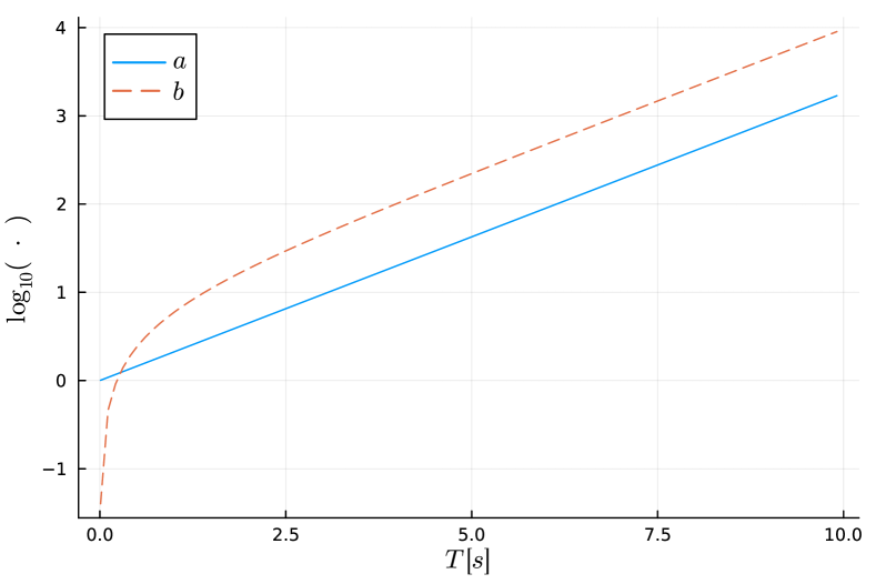
Figure 1: $\log(a)$ and $\log(b)$ with respect to $T$

Example 3

For the system given in Example 2, where $(1+L\alpha)=1.0075$, $\alpha M=0.040$ and $\Delta t=0.01$, let the number of $\Delta t$, i.e., $N$, equal to 2,000 providing the simulation time interval from 0 to $T$ equal to $20$s. Then,

$$\|{\boldsymbol{\phi}}_{2000}(20,0,{\bf x})-{\boldsymbol{\phi}}_{2000}(20,0,{\bf y})\|$$

$$\leq 1.0075^{2000}\|{\bf x}-{\bf y}\|+\sum_{r=0}^{1999}1.0075^{r}\times 0.010$$

$$\approx 3.27\times 10^{6}\|{\bf x}-{\bf y}\|+1.74\times 10^{7}$$ (23)

The values of $a$ and $b$ in the bounds calculated are large. For $T$ from 1 to 10 seconds, Figure 1 shows their values. They become several hundred already around $T=10$s, where $N=1000$.

In the following section, the bounds are improved by introducing the exponential stability assumption.

III Stability Verification

To reduce the bounds obtained in the previous section, the exponential stability condition is introduced.

Definition 2 (Exponential Stability)

The equilibrium point, ${\bf x}_{\text{eq}}={\bf 0}$, satisfying

$${\bf x}_{\text{eq}}={\bf x}_{\text{eq}}+\int^{\tau=t+\Delta t}_{\tau=t}{\bf f}[{\bf x}(\tau)]d\tau$$ (24)

for all $t\in[0,\infty)$, where ${\bf f}[{\bf x}(\tau)]$ is bounded by (10), is exponentially asymptotically stable if there exist positive constants, $r_{0}$, $k(\geq 1)$ and $\lambda$ such that

$$\|{\boldsymbol{\phi}}(t,t_{0},{\bf x}_{0})\|\leq k\|{\bf x}_{0}\|e^{-\lambda(t-t_{0})}$$ (25)

for all ${\bf x}_{0}={\bf x}(t_{0})\in{\mathbb{D}}_{0}$ and $t\geq t_{0}\geq 0$, where ${\mathbb{D}}_{0}=\{{\bf x}\in{\mathbb{R}}^{n}|\|{\bf x}\|\leq r_{0}\}$.

Finding the maximum $r_{0}$ satisfying the exponential stability and the size of the domain of attraction is of high interest in system stability verification.

Assumption 3 (Exponential Stable)

The nonlinear system given by (3) with the discontinuous function bounded by (10) is assumed to be exponentially stable at the equilibrium point, ${\bf x}_{\text{eq}}$, for all ${\bf x}_{0}\in{\mathbb{D}}_{0}$.

Theorem 4 (Exponential Bounds)

With the exponentially stable assumption, the following bound is satisfied:

$$\|{\boldsymbol{\phi}}_{N}(N\Delta t,t,{\bf x})-{\boldsymbol{\phi}}_{N}(N\Delta t,t,{\bf y})\|\leq 2kr_{0}e^{-\lambda T}$$ (26)

Proof: By the triangle inequality,

$$\|{\boldsymbol{\phi}}_{N}(N\Delta t,t,{\bf x})-{\boldsymbol{\phi}}_{N}(N\Delta t,t,{\bf y})\|$$

$$\leq\|{\boldsymbol{\phi}}_{N}(N\Delta t,t,{\bf x})\|+\|{\boldsymbol{\phi}}_{N}(N\Delta t,t,{\bf y})\|$$ (27)

Due to the exponential stable assumption and the definition of ${\mathbb{D}}_{0}$, the following inequalities are satisfied:

$$\|{\boldsymbol{\phi}}_{N}(N\Delta t,t,{\bf x})\|+\|{\boldsymbol{\phi}}_{N}(N\Delta t,t,{\bf y})\|$$

$$\leq k\|{\bf x}\|e^{-\lambda T}+k\|{\bf y}\|e^{-\lambda T}\leq 2kr_{0}e^{-\lambda T}$$ (28)

Hence, the inequality, (26), is satisfied.

$\blacksquare$

Theorem 5 (Square-root Bound)

The solution of the exponential stable nonlinear systems satisfies the following inequality:

$$\|{\boldsymbol{\phi}}_{N}(N\Delta t,t,{\bf x})-{\boldsymbol{\phi}}_{N}(N\Delta t,t,{\bf y})\|$$

$$\leq\sqrt{2kr_{0}e^{-\lambda T}a\|{\bf x}-{\bf y}\|+2kr_{0}e^{-\lambda T}b}$$ (29)

Proof: Multiplying the bound in (17) and the exponential bound in (26) and square-root both sides produces the inequality. $\blacksquare$

Example 4

For the nonlinear system given in Example 2, it is identified that $k=8/3$, $r_{0}=3/2$ and $\lambda=3$. The bounds for $|x_{0}|$ approaching $r_{0}$ with 1,000 simulation time histories are shown in Figure 2. Using the bound obtained in Example 3 with respect to $T$, the values of the square-root bound in (5) are shown in Figure 3. Both values become smaller than 0.001 around $T=5$s, where $N=500$.

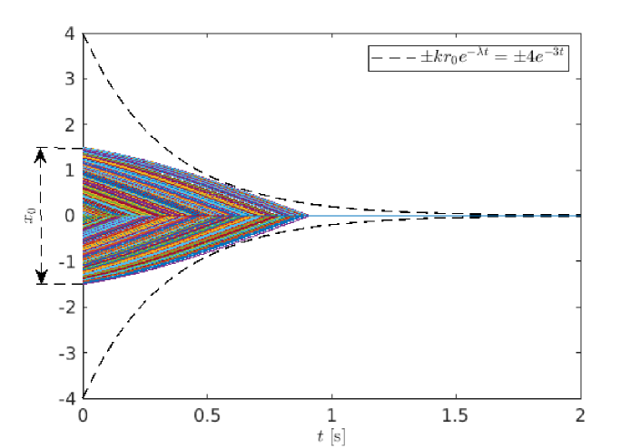
Figure 2: The exponential bounds and the 1000 Monte-Carlo simulations

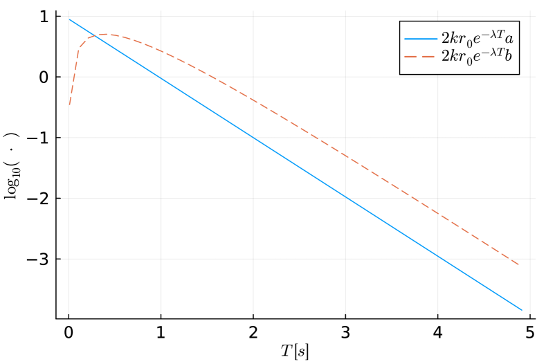
Figure 3: $\log_{10}(2kr_{0}e^{-\lambda T}a)$ and $\log_{10}(2kr_{0}e^{-\lambda T}b)$ with respect to $T$

Remark 2 (Choice of Simulation Time Interval $T$)

$T$ determines the time length of the numerical simulator. The longer $T$ requires a longer simulation time and the shorter $T$ results in larger values for the bound. The larger bound values require tighter samples, i.e., more samples, to check the stability conditions.

Definition 3 (Energy & Energy Integral)

The system energy, $E[{\boldsymbol{\phi}}_{N}(\tau,t,{\bf x}(t))]$, is defined by

$$E[{\boldsymbol{\phi}}_{N}(\tau,t,{\bf x}(t))]=\dfrac{1}{2}{\boldsymbol{\phi}}_{N}[\tau,t,{\bf x}(t)]^{T}P~{}{\boldsymbol{\phi}}_{N}[\tau,t,{\bf x}(t)]$$ (30)

where $P$ is an $n\times n$ positive-definite matrix, and the energy integral function, $V[t,{\bf x}(t)]$, is defined by

$$V[t,{\bf x}(t)]=\int^{t+T}_{t}E[{\boldsymbol{\phi}}_{N}(\tau,t,{\bf x}(t))]\,d\tau$$ (31)

Theorem 6 (Bounds of Energy & Energy Integral)

As the system is exponentially stable, the energy is bounded by

$$E[{\boldsymbol{\phi}}_{N}(\tau,t,{\bf x}(t))]\leq\dfrac{k_{E}}{2}k^{2}e^{-2\lambda(\tau-t)}\|{\bf x}(t)\|^{2}$$ (32)

where $k_{E}$ is the maximum eigenvalue of $P$, and the energy integral is bounded by

$$V[t,{\bf x}(t)]\leq T\dfrac{k_{E}}{2}k^{2}e^{-2\lambda(\tau-t)}\|{\bf x}(t)\|^{2}$$ (33)

Proof: The proof is trivial and omitted. $\blacksquare$

Example 5

For the nonlinear system given in Example 2 with the constants identified in Example 4, let the energy be given by

$$E(\tau,0,x_{0}) =\dfrac{1}{2}\phi^{2}_{150}(\tau,0,x_{0})$$

$$\leq\dfrac{1}{2}\left(\dfrac{8}{3}\right)^{2}e^{-6\tau}x^{2}_{0}=\dfrac{32}{9}e^{-6\tau}x^{2}_{0}$$

where $k_{E}=1$ and $x_{0}$ is the initial state in ${\mathbb{D}}_{0}$, and $V(t,x_{0})$ is bounded by $TE(\tau,0,x_{0})$.

Theorem 7 (Energy slope bound)

The energy function difference is bounded by

$$\left|E[{\boldsymbol{\phi}}_{N}(\tau,t,{\bf x})]-E[{\boldsymbol{\phi}}_{N}(\tau,t,{\bf y})]\right|$$

$$\leq k_{E}\sqrt{2kr_{0}e^{-\lambda T}a\|{\bf x}-{\bf y}\|+2kr_{0}e^{-\lambda T}b}$$ (34)

Proof: By the definition of the energy function, its slope, i.e., $\partial E/\partial{\boldsymbol{\phi}}$ is bounded by $k_{E}$. Hence, the difference is also bounded by

$$\left|E[{\boldsymbol{\phi}}_{N}(\tau,t,{\bf x})]-E[{\boldsymbol{\phi}}_{N}(\tau,t,{\bf y})]\right|$$

$$\leq k_{E}\left|{\boldsymbol{\phi}}_{N}(\tau,t,{\bf x})-{\boldsymbol{\phi}}_{N}(\tau,t,{\bf y})\right|$$ (35)

and due to the bound given by Theorem 5,

$$k_{E}\|{\boldsymbol{\phi}}_{N}(\tau,t,{\bf x})-{\boldsymbol{\phi}}_{N}(\tau,t,{\bf y})\|$$

$$\leq k_{E}\sqrt{2kr_{0}e^{-\lambda T}a\|{\bf x}-{\bf y}\|+2kr_{0}e^{-\lambda T}b}$$ (36)

$\blacksquare$

Example 6

For the nonlinear system given in Example 2 with the energy defined in Example 5, the energy slope bound is obtained as

$$\left|E[{\boldsymbol{\phi}}_{300}(3,0,x)]-E[{\boldsymbol{\phi}}_{300}(3,0,y)]\right|$$

$$\leq\sqrt{8e^{-9}\times 9.49|x-y|+8e^{-9}\times 45.27}$$

$$\approx\sqrt{0.0094|x-y|+0.0447}$$

where $N=300$ and $\Delta t=0.01$s.

Theorem 8 ($\delta$-sampling)

Choose ${\bf x}_{\delta}$ in ${\mathbb{S}}_{\delta}$ such that

$$\|{\bf x}-{\bf x}_{\delta}\|\leq\delta$$ (37)

where ${\mathbb{S}}_{\delta}$ is a finite subset of ${\mathbb{S}}$, ${\mathbb{S}}$ is a subset of ${\mathbb{R}}^{n}$. Then,

$$\left|E[{\boldsymbol{\phi}}_{N}(\tau,t,{\bf x})]-E[{\boldsymbol{\phi}}_{N}(\tau,t,{\bf x}_{\delta})]\right|$$

$$\leq k_{E}\sqrt{2kr_{0}e^{-\lambda T}a\|{\bf x}-{\bf x}_{\delta}\|+2kr_{0}e^{-\lambda T}b}$$

$$\leq k_{E}\sqrt{2kr_{0}e^{-\lambda T}a\delta+2kr_{0}e^{-\lambda T}b}$$ (38)

Definition 4 (Forward Invariant Set)

Let ${\mathbb{S}}$ be the set of ${\bf x}$, whose corresponding energy is less than $\ell$, i.e.,

$${\mathbb{S}}=\left\{{\bf x}|E({\bf x})\leq\ell\right\}$$ (39)

and the following inequality is satisfied for all ${\bf x}$ in ${\mathbb{S}}$

$$E[{\boldsymbol{\phi}}_{N}(T,0,{\bf x})]\leq\ell,$$ (40)

then the set ${\mathbb{S}}$ is forward invariant.

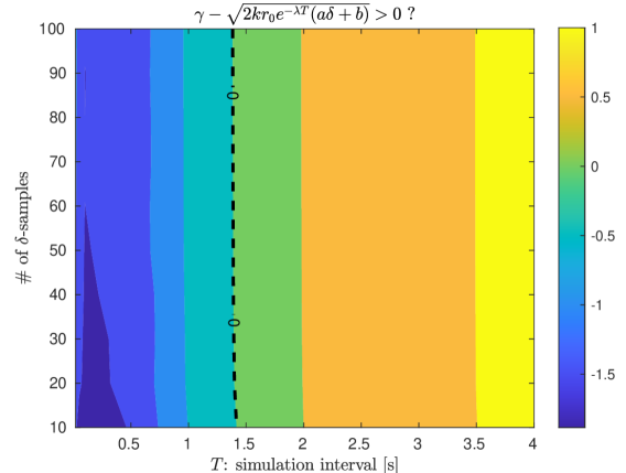
Figure 4: The inequality condition values for the ranges of the number of $x_{\delta}$ samplings and the simulation time length, $T$

Theorem 9 (Verification of Forward Invariant)

For all ${\bf x}_{\delta}$ in ${\mathbb{S}}_{\delta}$, if there exists a positive real $\gamma$ such that

$$E[{\boldsymbol{\phi}}_{N}(T,0,{\bf x}_{\delta})]\leq\ell-\gamma$$ (41)

and

$$\sqrt{2kr_{0}e^{-\lambda T}a\delta+2kr_{0}e^{-\lambda T}b}\leq\gamma,$$ (42)

then ${\mathbb{S}}$ is forward invariant [17].

Proof: Prove it by contradiction as in [17]. Assume (41) and (42) are satisfied but there exits ${\bf x}^{*}$ in ${\mathbb{S}}$ such that

$$E[{\boldsymbol{\phi}}_{N}(T,0,{\bf x}^{*})]>\ell\rightarrow-E[{\boldsymbol{\phi}}_{N}(T,0,{\bf x}^{*})]<-\ell$$ (43)

Add (41) and (43)

$$E[{\boldsymbol{\phi}}_{N}(T,0,{\bf x}_{\delta})]-E[{\boldsymbol{\phi}}_{N}(T,0,{\bf x}^{*})]<-\gamma<0$$ (44)

Hence,

$$\|E[{\boldsymbol{\phi}}_{N}(T,0,{\bf x}_{\delta})]-E[{\boldsymbol{\phi}}_{N}(T,0,{\bf x}^{*})]\|>\gamma$$ (45)

Because of the energy slope bound in (7)

$$\gamma <\|E[{\boldsymbol{\phi}}_{N}(T,0,{\bf x}_{\delta})]-E[{\boldsymbol{\phi}}_{N}(T,0,{\bf x}^{*})]\|$$

$$\leq k_{E}\sqrt{2kr_{0}e^{-\lambda T}a\|{\bf x}_{\delta}-{\bf x}^{*}\|+2kr_{0}e^{-\lambda T}b}$$ (46)

As ${\bf x}_{\delta}$ belongs to the $\delta$-sampling set, ${\mathbb{S}}_{\delta}$ in Theorem 8,

$$\gamma <\|E[{\boldsymbol{\phi}}_{N}(T,0,{\bf x}_{\delta})]-E[{\boldsymbol{\phi}}_{N}(T,0,{\bf x}^{*})]\|$$

$$\leq k_{E}\sqrt{2kr_{0}e^{-\lambda T}a\|{\bf x}_{\delta}-{\bf x}^{*}\|+2kr_{0}e^{-\lambda T}b}$$

$$\leq k_{E}\sqrt{2kr_{0}e^{-\lambda T}a\delta+2kr_{0}e^{-\lambda T}b}$$ (47)

The right-most term is bounded by (42) and finally,

$$\gamma<\|E[{\boldsymbol{\phi}}_{N}(T,0,{\bf x}_{\delta})]-E[{\boldsymbol{\phi}}_{N}(T,0,{\bf x}^{*})]\|\leq\gamma$$ (48)

The inequality contradicts. Hence, the assumption of the existence of ${\bf x}^{*}$ is incorrect.

$\blacksquare$

Algorithm 1 Stability Verification with $\delta$-Samples

1:Set $\Delta t$, $N$, $\delta$, $k$, $\lambda$ and $\ell$

2:Generate ${\bf x}_{\delta}\in{\mathbb{S}}_{\delta}\subset{\mathbb{S}}$

3:while True do

4:     Run Simulator for each ${\bf x}_{\delta}$

5:     Calculate $\gamma=\ell-\max E[{\boldsymbol{\phi}}_{N}(T,0,{\bf x}_{\delta})]$

6:     if $\gamma>0$ then

7:         if (42) satisfies then

8:              if all ${\bf x}_{\delta}$ checked then ${\mathbb{S}}$ is forward-invariant.

9:              else go to the next sample

10:              end if

11:         else reduce $\delta$ and go to ${\bf x}_{\delta}$ generation

12:         end if

13:     else adjust $N$, $\delta$, $k$, $\lambda$ and $\ell$ and start over

14:     end if

15:end while

Example 7

For the nonlinear system given in Example 2 with the energy difference bound in Example 6, the inequality for $\delta$ and $\gamma$ must satisfy as follows:

$$\sqrt{0.0094|x-y|+0.0447}\leq\gamma$$

The inequality provides the minimum $\gamma$ bound equal to 0.0447, where $\delta$ is equal to zero corresponding to the infinitely many samples. As $(\ell-\gamma)$ in (41) must be positive, the smaller minimum $\gamma$ increases the chance that the inequality in (41) satisfies with a positive value of $\delta$, i.e., a finite number of samples. Change $N=400$, i.e., $T=4$s, then the following inequality is calculated

$$\sqrt{0.0009\delta+0.005}\leq\gamma$$

and the lower bound of the minimum $\gamma$ is reduced to 0.005.

Algorithm 1 summarizes the stability check using a finite number of samples.

Remark 3

Overestimating $k$, which is related to overshoots of the response, in the Algorithm is allowed with the price that longer simulation time interval, i.e., larger, $N$, would need to satisfy the inequalities. On the other hand, $\lambda$ must be underestimated.

Example 8

For Example 2, each variable in Algorithm 1 is given by $\Delta t=0.01$, $k=8/3$, $\lambda=3$ and $\ell=(k_{E}r_{0}^{2})/2$, where $k_{E}=1.0$ and $r_{0}=3/2$. $N$ varies from 10 to 100. $T$ is determined by $N\Delta t$. For each $N$, $N_{\text{samp}}$ number of $x_{\delta}$ samples are obtained in $-r_{0}<x_{\delta}<r_{0}$, while the maximum distance between the samples is kept less than $\delta/2$. The $\gamma$ inequality condition for each combination of the number of $x_{\delta}$ samples and $T$ is shown in Figure 4. For this example, when the stability inequality condition is violated, it is better to increase $T$ instead of decreasing $\delta$.

IV Conclusions & Future Works

We present a stability verification method providing the deterministic stability assurance of dynamical systems implemented as high-fidelity numerical simulators, which may include hard nonlinear components such as discontinuous jumps in the states and magnitude/speed constraints, and simulation-based control design algorithms such as reinforcement learning, which does not provide a stability guarantee by the design procedures. For each specific real-world application, there would be abundant room to improve the proposed algorithm in terms of a parallelization of the algorithm, an efficient sampling and a better estimation of $k$ and $\lambda$ leading to allow the larger $\delta$ and/or the smaller $\gamma$. For example, [18] provides the way of efficient sampling.

References

[1]
N. Lehtomaki, N. Sandell, and M. Athans, “Robustness results in
linear-quadratic gaussian based multivariable control designs,” IEEE
Transactions on Automatic Control, vol. 26, no. 1, pp. 75–93, 1981.
[2]
J. Doyle, K. Glover, P. Khargonekar, and B. Francis, “State-space solutions to
standard and control problems,” IEEE Transactions
on Automatic Control, vol. 34, no. 8, pp. 831–847, 1989.
[3]
V. Utkin, “Variable structure systems with sliding modes,” IEEE
Transactions on Automatic Control, vol. 22, no. 2, pp. 212–222, 1977.
[4]
M. Morari and J. H. Lee, “Model predictive control: past, present and
future,” Computers & chemical engineering, vol. 23, no. 4-5, pp.
667–682, 1999.
[5]
J. Kapinski, J. V. Deshmukh, X. Jin, H. Ito, and K. Butts, “Simulation-based
approaches for verification of embedded control systems: An overview of
traditional and advanced modeling, testing, and verification techniques,”
IEEE Control Systems Magazine, vol. 36, no. 6, pp. 45–64, 2016.
[6]
S. Karimi, P. Poure, and S. Saadate, “A HIL-based reconfigurable platform
for design, implementation, and verification of electrical system digital
controllers,” IEEE Transactions on Industrial Electronics, vol. 57,
no. 4, pp. 1226–1236, 2010.
[7]
S. Chen, Y. Chen, S. Zhang, and N. Zheng, “A novel integrated simulation and
testing platform for self-driving cars with hardware in the loop,”
IEEE Transactions on Intelligent Vehicles, vol. 4, no. 3, pp.
425–436, 2019.
[8]
D. H. Lee, C.-J. Kim, and S. H. Lee, “Development of unified high-fidelity
flight dynamic modeling technique for unmanned compound aircraft,”
International Journal of Aerospace Engineering, vol. 2021, pp. 1–23,
2021.
[9]
J. V. Foster and D. Hartman, “High-fidelity multi-rotor unmanned aircraft
system (UAS) simulation development for trajectory prediction under
off-nominal flight dynamics,” in 17th AIAA Aviation Technology,
Integration, and Operations Conference, 2017, p. 3271.
[10]
B. Hieb, “Creating a high-fidelity model of an electric motor for control
system design and verification,” Technical Article Published by The
MathWorks, 2013.
[11]
R. S. Sutton, A. G. Barto et al., “Reinforcement learning,”
Journal of Cognitive Neuroscience, vol. 11, no. 1, pp. 126–134, 1999.
[12]
T. P. Lillicrap, J. J. Hunt, A. Pritzel, N. Heess, T. Erez, Y. Tassa,
D. Silver, and D. Wierstra, “Continuous control with deep reinforcement
learning,” arXiv preprint arXiv:1509.02971, 2015.
[13]
M. Vukobratovic, V. Potkonjak, and V. Matijevic, Dynamics of robots with
contact tasks. Springer Science &
Business Media, 2003, vol. 26.
[14]
H. K. Khalil, Nonlinear control. Pearson New York, 2015, vol. 406.
[15]
J. Trumpf and R. Mahony, “A converse liapunov theorem for uniformly locally
exponentially stable systems admitting Carathèodory solutions,”
IFAC Proceedings Volumes, vol. 43, no. 14, pp. 1374–1378, 2010.
[16]
J. Cortes, “Discontinuous dynamical systems,” IEEE Control Systems
Magazine, vol. 28, no. 3, pp. 36–73, 2008.
[17]
J. Kapinski and J. Deshmukh, “Discovering forward invariant sets for nonlinear
dynamical systems,” in Interdisciplinary Topics in Applied
Mathematics, Modeling and Computational Science, M. G. Cojocaru, I. S.
Kotsireas, R. N. Makarov, R. V. N. Melnik, and H. Shodiev, Eds. Cham: Springer International Publishing, 2015,
pp. 259–264.
[18]
R. Bobiti and M. Lazar, “Automated-sampling-based stability verification and
doa estimation for nonlinear systems,” IEEE Transactions on Automatic
Control, vol. 63, no. 11, pp. 3659–3674, 2018.