Optimal Locally Private Nonparametric Classification
with Public Data
Abstract
In this work, we investigate the problem of public data-assisted non-interactive LDP (Local Differential Privacy) learning with a focus on non-parametric classification. Under the posterior drift assumption, we for the first time derive the mini-max optimal convergence rate with LDP constraint. Then, we present a novel approach, the locally private classification tree, which attains the mini-max optimal convergence rate. Furthermore, we design a data-driven pruning procedure that avoids parameter tuning and produces a fast converging estimator. Comprehensive experiments conducted on synthetic and real datasets show the superior performance of our proposed method. Both our theoretical and experimental findings demonstrate the effectiveness of public data compared to private data, which leads to practical suggestions for prioritizing non-private data collection.
1 Introduction
Local differential privacy (LDP) [KOV14, DJW18], which is a variant of differential privacy (DP) [Dwo+06], has gained considerable attention in recent years, particularly among industrial developers [EPK14, Tan+17]. Unlike central DP, which relies on a trusted curator who has access to the raw data, LDP assumes that each sample is possessed by a data holder, and each holder privatizes their data before it is collected by the curator. Although this setting provides stronger protection, learning with perturbed data requires more samples [DJW18] compared to the central setting. Moreover, basic techniques such as principal component analysis [WX20, BKS22], data standardization [BKS22], and tree partitioning [Wu+22] are troublesome or even prohibited. Consequently, LDP introduces challenges for various machine learning tasks that are otherwise considered straightforward, including density estimation [DJW13], mean estimation [DJW18], Gaussian estimation [Jos+19], and change-point detection [BY21].
Fortunately, in certain scenarios, private estimation performance can be enhanced with an additional public dataset. From an empirical perspective, numerous studies demonstrated the effectiveness of using public data [Pap+17, Pap+18, Yu+21a, Yu+22, Nas+23, GKW23]. In most cases, the public data is out-of-distribution and collected from other related sources. Yet, though public data from an identical distribution has been extensively studied [BTG18, ABM19, Kai+21, Ami+22, Ben+23, Low+23, Wan+23], only a few works systematically described the out-of-distribution relationship. Focusing on unsupervised problems, i.e. Gaussian estimation, [BKS22] discussed the gain of using public data with respect to the total variation distance between private and public distributions. As for supervised learning, [GKW23] discussed the similarities between datasets to guide the selection of appropriate public data. [Ma+23] leveraged public data to create informative partitions for LDP regression trees. Neither of them discussed the relationship between regression functions of private and public distributions. Aiming at the gap between theory and practice in supervised private learning with public data, we pose the following intriguing questions:
| 1. Theoretically, when is labeled public data beneficial for LDP learning? |
| 2. Under such conditions, how to effectively leverage public data? |
Moreover, leveraging public data necessitates more complex models, which often results in an increased number of hyperparameters to tune. Hyper-parameter tuning is an essential yet challenging task in private learning [PS21, Moh+22]. Consequently, models with public data may face difficulties in parameter selection, which leads to the third consideration:
| 3. Can data-driven hyperparameter tuning approaches be derived? |
In this work, we answer the above questions from the perspective of non-parametric classification with the non-interactive LDP constraint. Though parametric methods enjoy better privacy-utility trade-off [DJW18] under certain assumptions, they are vulnerable to model misspecification. Under LDP setting where we have limited prior knowledge of the data, non-parametric methods ensure the worst-case performance. As for private classification, the local setting remains rarely explored compared to the central setting. A notable reason is that most gradient-based methods [SCS13, Aba+16] are prohibited due to the high demand for memory and communication capacity on the terminal machine [TKC22]. We consider non-interactive LDP, where the communication between the curator and the data holders is limited to a single round. This type of method is favored by practitioners [STU17, ZMW17, DF19] since they avoid multi-round protocols that are prohibitively slow in practice due to network latency.
Under such background, we summarize our contributions by answering the questions:
-
•
For the first question, we propose to adopt the framework of posterior drift, a setting in transfer learning [Men+15, CW21], for our analysis. Specifically, given the private distribution and the public distribution , we require , i.e. they have the same marginal distributions. Moreover, their Bayes decision rule are identical, i.e. . The assumption covers a wide range of distributions and includes as a special case. Theoretically, we for the first time establish a mini-max lower bound for nonparametric LDP learning with public data.
-
•
To answer the second question, we propose the Locally differentially Private Classification Tree (LPCT), a novel algorithm that leverages both public and private data. Specifically, we first create a tree partition on public data and then estimate the regression function through a weighted average of public and private data. Besides inheriting the merits of tree-based models such as efficiency, interpretability, and extensivity to multiple data types, LPCT is superior from both theoretical and empirical perspectives. Theoretically, we show that LPCT attains the mini-max optimal convergence rate. Empirically, we conduct experiments on both synthetic and real datasets to show the effectiveness of LPCT over state-of-the-art competitors.
-
•
To answer the last question, we propose the Pruned Locally differentially Private Classification Tree (LPCT-prune), a data-driven classifier that is robust to its parameter setting. Specifically, we query the privatized information with a sufficient tree depth and conduct an efficient pruning procedure. Theoretically, we show that LPCT-prune achieves the optimal convergence rate in most cases and maintains a reasonable convergence rate otherwise. Empirically, we illustrate that LPCT-prune with a default parameter performs comparable to LPCT with the best parameters.
This article is organized as follows. In Section 2, we provide a comprehensive literature review. Then we formally define our problem setting and introduce our methodology in Section 3. The obtained theoretical results are presented in Section 4. Then we develop the data-driven estimator in Section 5. Extensive experiments are conducted on synthetic data and real data in Section 6 and 7 respectively. The conclusion and discussions are in Section 8.
2 Related work
2.1 Private learning with public data
Leveraging public data in private learning is a research topic that is both theoretically and practically meaningful to closing the gap between private and non-private methods. There is a long list of works addressing the issue of private learning with public data from a central differential privacy perspective. Through unlabeled public data, [Pap+17, Pap+18] fed knowledge privately into student models, whose theoretical benefits are established by [Liu+21]. Empirical investigations have demonstrated the effectiveness of pretraining on public data and fine-tuning privately on sensitive data [Li+22, Yu+22, Gan+23, Yu+23]. Using the information obtained in public data, [WZ20, Kai+21, Yu+21, ZWB21, Ami+22, Nas+23] investigated preconditioning or adaptively clipping the private gradients, which reduce the required amount of noise in DP-SGD and accelerate its convergence. Theoretical works such as [BTG18, ABM19, Bas+20] studied sample complexity bounds for PAC learning and query release based on the VC dimension of the function space. [BKS22] used public data to standardize private data and showed that the sample complexity of Gaussian mean estimation can be augmented in the sense of the range parameter. More recently, by relating to sample compression schemes, [Ben+23] presented sample complexities for several problems including Gaussian mixture estimation. [Gan+23] explained the necessity of public data by investigating the loss landscape.
In contrast, there is less attention focused on the local setting. [SXW23] considered half-space estimation with an auxiliary unlabeled public data. They construct several weak LDP classifiers and label the public data by majority vote. They established sample complexity that is linear in the dimension and polynomial in other terms for both private and public data. [Wan+23] employed public data to estimate the leading eigenvalue of the covariance matrix, which will serve as a reference for data holders to clip their statistics. Given the learned clipping threshold, the sample complexity for GLM with LDP for a general class of functions is improved to polynomial concerning error, dimension, and privacy budget, which is shown impossible without public data [STU17, DF20]. Both [Wan+23] and [SXW23] considered the unlabeled data, while our work further leverages the information contained in the labels if labeled public data is available. More recently, [Ma+23] enhanced LDP regression by using public data to create an informative partition. However, the relationship between the public and private distribution is vaguely defined. Also, their theoretical results are no better than using just private data. [Low+23] studied mean estimation, DP-SCO, and DP-ERM with public data. They assume that the public data and the private data are identically distributed. Also, the theoretical results are established under sequential-interactive LDP. Despite the distinctions in the research problem, their conclusions are analogous to ours: the asymptotic optimal error can be achieved by using either the private or public estimation solely, while weighted average estimation achieves better constant as well as empirical performance.
2.2 Locally private classification
LDP classification with parametric assumptions can be viewed as a special case of LDP-ERM [STU17, ZMW17, WGX18, DF19, WSX19, DF20, Wan+20, Wan+23]. Most works provide evidence of hardness on non-interactive LDP-ERM. Non-parametric methods possess a worse privacy-utility trade-off [DJW18] and are considered to be harder than parametric problems. [ZMW17] investigated the kernel ridge regression and established a bound of estimation error of the order . Their results only apply to losses that are strongly convex and smooth. The works most related to ours is that of [BB19, BGW21]. [BB19] studied non-parametric classification with the hölder smoothness assumption. They proposed a histogram-based method using the Laplace mechanism and showed that this approach is mini-max optimal under their assumption. The strong consistency of this approach is established in [BGW21] as a by-product. Our results include their conclusion as a special case and hold in a stronger sense, i.e. “uniformly with high probability” instead of “in expectation”.
2.3 Private hyperparameter tuning
Researchers highlighted the importance and difficulty of parameter tuning under DP constraint [PS21, Wan+23a] focusing on central DP. [CV13] explored this problem under strong stability assumptions. [LT19] presented DP algorithms for selecting the best parameters in several candidates, which is closely related to the DP selection [MT07]. Compared to the original algorithm, their method suffers a factor of 3 in the privacy parameter, meaning that 2/3 of the privacy budget is spent on the selection process. [PS21] improved the result with a much tighter privacy bound in Renyi-DP by running the algorithm random times and returning the best result. Recently, [Wan+23a] proposed a framework that reduces DP parameter selection to a non-DP counterpart. This approach leverages existing hyperparameter optimization methods and outperforms the uniform sampling approaches [LT19, PS21]. [Ram+20] proposed to tune hyperparameters on public datasets. [Moh+22] argued that, under a limited privacy budget, DP optimizers that require less tuning are preferable. As far as we know, there is a lack of research focusing on the LDP parameter selection, whether in an interactive or non-interactive context.
3 Locally differentially private classification tree
In this section, we introduce the Locally differentially Private Classification Tree (LPCT). After explaining necessary notations and problem setting in Section 3.1, we propose our decision tree partition rule in Section 3.2. Finally, Section 3.3 introduces our privacy mechanism and proposes the final algorithm.
3.1 Problem setting
We introduce necessary notations. For any vector , let denote the -th element of . Recall that for , the -norm of is defined by . Throughout this paper, we use the notation and to denote that there exist positive constant and such that and , for all . In addition, we denote if and . Let and . Besides, for any set , the diameter of is defined by . Let the standard Laplace random variable have probability density function for .
It is legitimate to consider binary classification while an extension of our results to multi-class classification is straightforward. Suppose there are two unknown probability measures, the private measure and the public measure on . We observe i.i.d. private samples drawn from the private distribution , and i.i.d. public samples drawn from the public distribution . The data points from the distributions and are also mutually independent. Our goal is to classify under the private distribution . Given the observed data, we construct a classifier which minimizes the classification risk under the target distribution :
Here means the probability when are drawn from distribution . The Bayes risk, which is the smallest possible risk with respect to , is given by . In such binary classification problems, the regression functions are defined as
| (1) |
which represent the conditional distributions and . The function that achieves Bayes risk with respect to is called Bayes function, namely, .
We consider the following setting. The estimator is considered as a random function with respect to both and , while its construction process with respect to is locally differentially private (LDP). The rigorous definition of LDP is as follows.
Definition 1 (Local Differential Privacy).
Given data , each is mapped to privatized information which is a random variable on . Let be the -field on . is drawn conditional on via the distribution for . Then the mechanism provides -local differential privacy (-LDP) if
Moreover, if is observed by a single query to , then is non-interactive -LDP.
This formulation is widely adopted [DJW13, BB19]. In contrast to central DP where the likelihood ratio is taken concerning some statistics of all data, LDP requires individuals to guarantee their own privacy by considering the likelihood ratio of each . Once the view is provided, no further processing can reduce the deniability about taking a value since any outcome is nearly as likely to have come from some other initial value .
Besides the privacy guarantee of data, we consider the existence of additional public data from distribution . To depict the relationship between and , we consider the posterior drift setting in transfer learning literature [Men+15, CW21]. Under the posterior drift model, let be the identical marginal distribution. The main difference between and lies in the regression functions and . Specifically, let for some strictly increasing link function with . The condition that is strictly increasing leads to the situation where those that are more likely to be labeled under are also more likely to be labeled under . The assumption guarantees that those that are non-informative under are the same under , and most importantly, the sign of and are identical.
3.2 Decision tree partition
In this section, we formalize the decision tree partition process. A binary tree partition is a disjoint cover of obtained by recursively split grids into subgrids. While our methodology applies to any tree partition, it can be challenging to use general partitions such as the original CART [Bre84] for theoretical analysis. Following [Cai+23, Ma+23], we propose a new splitting rule called the max-edge partition rule. This rule is amenable to theoretical analysis and can also achieve satisfactory practical performance. In the non-interactive setting, the private dataset is unavailable during the partition process and the partition is created solely on the public data. Given public dataset , the partition rule is stated as follows:
-
•
Let be the initial rectangular cell and be the initialized cell partition. stands for the initialized index set. In addition, let represent the maximum depth of the tree. The parameter is fixed beforehand by the user and possibly depends on .
-
•
Suppose we have obtained a partition of after steps of the recursion. Let . In the -th step, for each , , suppose it is . If there is no sample in , no operation is done and let . Otherwise, we choose the edge to be split among the longest edges. The index set of longest edges is defined as
-
•
Assume we split along the -th dimension for , is then partitioned into a left sub-cell and a right sub-cell along the midpoint of the chosen dimension, where and . Then the dimension to be split is chosen using the variance reduction criterion:
(2) where the function can be criteria for decision tree classifiers such as the Gini index or information gain.
-
•
Once is selected, let .
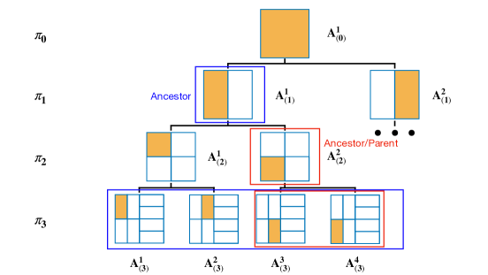
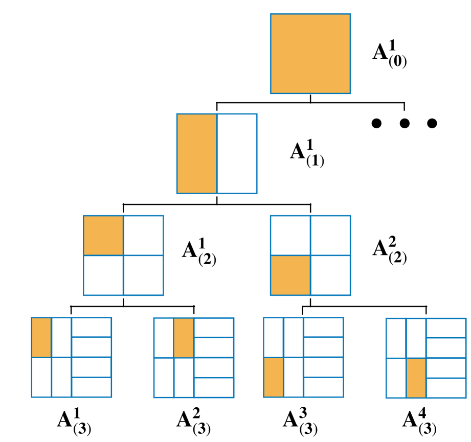
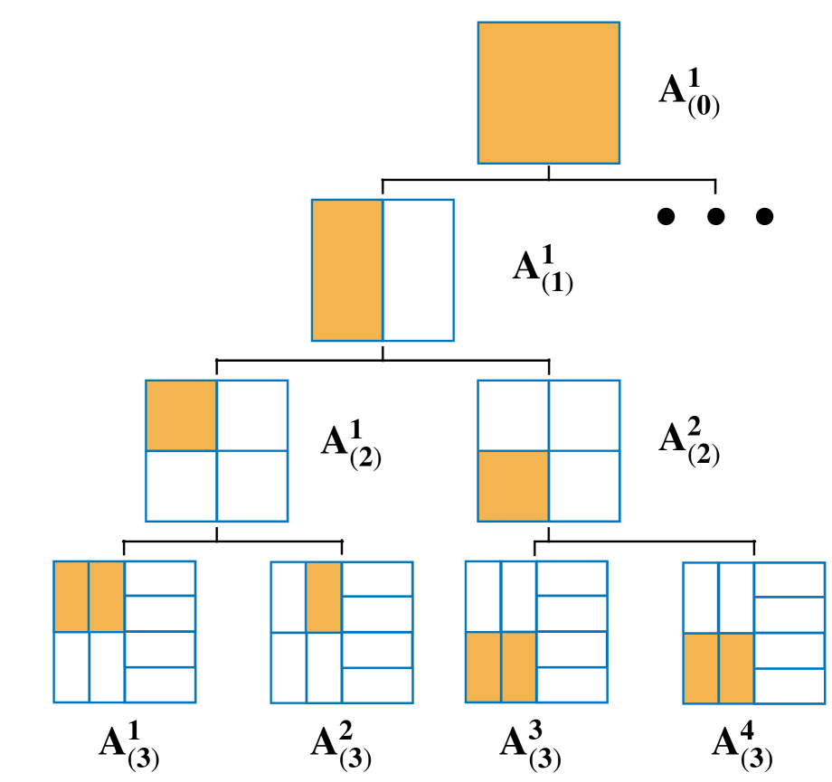
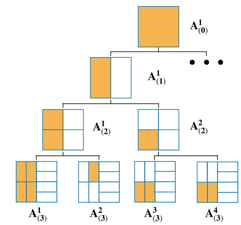
The complete process is presented in Algorithm 1 and illustrated in Figure 1. For each grid, the partition rule selects the midpoint of the longest edges that achieves the largest score reduction. This procedure continues until either node has no samples or the depth of the tree reaches its limit. We also define relationships between nodes which are necessary in Section 5. For node , we define its parent node as
For , the ancestor of a node with depth is then defined as
which is the grid in that contains .
3.3 Privacy mechanism for any partition
This section focuses on the privacy mechanism based on general tree partitions. We first introduce the necessary definitions and then present our private estimation based on the Laplacian mechanism in (8). To avoid confusion, we refer the readers to a clear summarization of the defined estimators in Appendix A.1.
For index set , let be the tree partition created by Algorithm 1. A population classification tree estimation is defined as
| (3) |
The label is inferred using the population tree classifier which is defined as . Here, we let by definition.
To get an empirical estimator given the data set , we estimate the numerator and the denominator of (3) separately. To estimate the denominator, each sample contributes a one-hot vector where the -th element of is . Then an estimation of is , which is the number of samples in divided by . Analogously, let . An estimation of is , which is the sum of the labels in divided by . Combining the pieces, a classification tree estimation is defined as
| (4) |
The corresponding classifer is defined as . In other words, estimates by the average of the responses in the cell. In the non-private setting, each data holder prepares and according to the partition and sends it to the curator. Then the curator aggregates the transmission following (4).
To protect the privacy of each data, we propose to estimate the numerator and denominator of the population regression tree using a privatized method. Specifically, and are combined with the Laplace mechanism [Dwo+06] before being sent to the curator. For i.i.d. standard Laplace random variables and , let
| (5) |
Then a privatized estimation of is . Analogously, let
| (6) |
An estimation of is . Then using the privatized information , we can estimate the regression function as
| (7) |
The procedure is also derived by [BB19]. As an alternative, one can use random response [War65] since both and are binary vectors. The following proposition shows that the estimation procedures satisfy LDP.
Proposition 2.
In the case where one also has access to the -data in addition to the -data, the data can be used to help the classification task under the target distribution and should be taken into consideration. The utilization of data must satisfy the local DP constraint while the data can be arbitrarily adopted. We accommodate the existing private estimation (7) and non-private estimation (4) by taking a weighted average based on both estimators. Denote the encoded information from and as and , respectively. We use the same partition for estimator and estimator. Namely, (4) and (7) are constructed via an identical . When taking the average, data from the different distributions should have different weights since the signal strengths are different between and . To make the classification at , the Locally differentially Private Classification Tree estimation (LPCT) is defined as follows:
| (8) |
Here, we let . The locally private tree classifier is . In each leaf node , the classifier is assigned a label based on the weighted average of estimations from and data. The parameter serves to balance the relative contributions of both and . A higher value of indicates that the final predictions are predominantly influenced by the public data, and vice versa.
4 Theoretical results
In this section, we present the obtained theoretical results. We present the matching lower and upper bounds of excess risk in Section 4.1 and 4.2. Finally, we demonstrate that LPCT is free from the unknown range parameter in Section 4.3. All technical proofs can be found in Appendix B.
4.1 Mini-max convergence rate
We first give the necessary assumptions on the distribution and . Then we provide the mini-max rate under the assumptions.
Assumption 3.
Let . Assume the regression function is -Hölder continuous, i.e. there exists a constant such that for all , . Also, assume that the marginal density functions of and are upper and lower bounded, i.e. for some .
Assumption 4 (Margin Assumption).
Let . Assume
Assumption 5 (Relative Signal Exponent).
Let the relative signal exponent and . Assume that
Assumption 3 and 4 are standard conditions that have been widely used for non-parametric classification problems [AT07, Sam12, CD14]. Assumption 5 depicts the similarity between the conditional distribution of public data and private data. When is small, the signal strength of is strong compared to . In the extreme instance of , consistently remains distant from by a constant. In contrast, when is large, there is not much information contained in . The special case of allows to always be and is thus non-informative. We present the following theorem that specifies the mini-max lower bound with LDP constraints on data under the above assumptions. The proof is based on first constructing two function classes and then applying the information inequalities for local privacy [DJW18] and Assouad’s Lemma [Tsy09].
Theorem 6.
If , our results reduce to the special case of LDP non-parametric classification with only private data. In this case, the mini-max lower bound is of the order . Previously, [BB19] provided an estimator that reaches the mini-max optimal convergence rate. If , the result recovers the learning rate established for transfer learning under posterior drift [CW21]. In this case, we have only source data from and want to generalize the classifier on the target distribution .
The mini-max convergence rate (9) is the same as if one fits an estimator using only data with sample size . The contribution of data is substantial when . Otherwise, the convergence rate is not significantly better than using data only. The quantity , which is referred to as effective sample size, represent the theoretical gain of using data with sample size under given , and . Notably, the smaller is, the more effective the data becomes, and the greater gain is acquired by using data. Regarding different values of , our work covers the setting in previous work when a small amount of effective public samples are required [BKS22, Ben+23], and when a large amount of noisy/irrelevant public samples are required [Yu+21a, Gan+23, Yu+23]. Also, the public data is more effective for small , i.e. under weaker privacy constraints. Compared to the effective sample size of the two-sample classifier in [CW21] which is , our effective sample size is much larger. As an interpretation, compared to transfer learning in the non-private setting, public data becomes more valuable in the private setting.
4.2 Convergence rate of LPCT
In the following, we show the convergence rate of LPCT reaches the lower bound with proper parameters. The proof is based on a carefully designed decomposition in Appendix B.3. Define the quantity
| (10) |
Theorem 7.
Let be constructed through the max-edge partition in Section 3.2 with depth . Let be the locally private two-sample tree classifier. Suppose Assumption 3, 4, and 5 hold. Then, for , if and , there holds
| (11) |
with probability with respect to where is the joint distribution of privacy mechanisms in (5) and (6).
Compared to Theorem 6, the LPCT with the best parameter choice reaches the mini-max lower bound up to a logarithm factor. Both parameters and should be assigned a value of the correct order to achieve the optimal trade-off. The depth increases when either or grows. This is intuitively correct since the depth of a decision tree should increase with a larger number of samples. The strength ratio , on the other hand, is closely related to the value of . As explained earlier, a small guarantees a stronger signal in . Thus, the value of is decreasing for . In this case, when the signal strength of is large, we rely more on the estimation by data by assigning a larger ratio to it.
We note that when is large, there is a gap between in the lower bound and in the upper bound. The problem can be mitigated by employing the random response mechanism [War65] instead of the Laplace mechanism, as mentioned in Section 3.3. The theoretical analysis generalizes analogously, see e.g. [Ma+23]. Here, we do not address this issue as we want to focus on public data. The theorem restricts . When , the estimator is drastically perturbed by the random noise and the convergence rate is no longer optimal. As gets larger, the upper bound of excess risk decreases until . When , the random noise is negligible and the convergence rate remains to be
which recovers the rate of non-private learning as established in [CW21].
We discuss the order of ratio . When , we have . This rate is exactly the same as in the conventional transfer learning case [CW21] and is enough to achieve the optimal trade-off. Yet, under privacy constraints, this choice of will fail when . Roughly speaking, if we let in this case, there is a probability such that the noise in (8) will dominate the non-private density estimation . When the domination happens, the point-wise estimation is decided by random noises, and thus the overall excess risk fails to converge. To alleviate this issue, we assign a larger value to ensure . As an interpretation, in the private setting, we place greater reliance on the estimation by public data compared to the non-private setting.
Last, we discuss the computational complexity of LPCT. We first consider the average computation complexity of LPCT. The training stage consists of two parts. Similar to the standard decision tree algorithm [Bre84], the partition procedure takes time. The computation of (8) takes time. From the proof of Theorem 7, we know that , where . Thus the training stage complexity is around which is sub-linear. Since each prediction of the decision tree takes time, the test time for each test instance is no more than . As for storage complexity, since LPCT only requires the storage of the tree structure and the prediction value at each node, the space complexity of LPCT is which is also sub-linear. In short, LPCT is an efficient method in time and memory.
4.3 Eliminating the range parameter
We discuss how public data can eliminate the range parameter contained in the convergence rate. When is unknown, one must select a predefined range for creating partitions. Only then do the data holders have a reference for encoding their information. In this case, the convergence rate of [BB19] becomes , which is slower than the known for any . A small means that a large part of the informative will be ignored (the second term is large), whereas a large may create too many redundant cells (the first term is large). See [GK22] for detailed derivation. Without much prior knowledge, this parameter can be hard to tune. The removal of the range parameter is first discussed in [BKS22], where public data is required. Our result shows that we do not need to tune this range parameter with the help of public data.
Theorem 8.
Suppose the domain is unknown. Let and . Define the min-max scaling map where . The the min-max scaled and is written as and . Then for trained within on and as in Theorem 7, we have
with probability with respect to .
5 Data-driven tree structure pruning
Parameter tuning stands as an essential issue in differential privacy [LT19, PS21, Moh+22, Low+23] and remains an unsolved problem in local differential privacy. Common strategies, such as cross-validation and information criteria, remain unavailable due to their requirement for multiple queries to the training data. Tuning by omitting a validation set is restrictive in terms of the size of the potential hyperparameter space [Ma+23]. Hence, an available parameter tuning procedure is indispensable for a locally private model.
In terms of LPCT, there are two parameters, the depth and the relative ratio , both of which have an optimal value depending on the unknown and . We do not select a global parameter. Instead, we first query the privatized information with a sufficient tree depth . Then, we introduce a greedy procedure to locally prune the tree to an appropriate depth and select based on local information. This scheme is beneficial from two perspectives: (1) This procedure avoids multiple queries to the data and works under the non-interactive setting, i.e. each data holder only sends their privatized message once. (2) This procedure avoids the tuning of sensitive parameters and . Instead, it only requires a predefined parameter, . Furthermore, the performance of the pruned estimator is insensitive to . The estimator achieves satisfactory results over a wide range of , making it feasible to select a default value. As a result, we do not specifically waste any privacy budget on parameter selection. However, there is a reasonable drop in performance compared to the model with the best parameters.
Below, in Section 5.1, we derive a selection scheme in the spirit of Lepski’s method [Lep92], a classical method for adaptively choosing the hyperparameter. Yet, we show this method fails in the presence of privacy protection. In Section 5.2, we make slight modifications to the scheme and illustrate the effectiveness of the amended approach.
5.1 A naive strategy
For max-edge partition with depth and node , the depth ancestor private tree estimation is defined as
| (12) |
and consequently the classifier is defined as . See Figure 2(a) for an illustration of estimation at ancestor nodes. We provide a preliminary result that will guide the derivation of the pruning procedure in the following proposition.
Proposition 9.
Let be constructed through the max-edge partition in Section 3.2 with depth . Let be the tree estimator with depth ancestor node in (12). Suppose Assumption 3 holds. Define the quantity
| (13) |
where the summation over is with respect to all descendent nodes of the depth- ancestor, i.e. . The constant is specified in the proof. Then, for all and , if there holds
with probability with respect to where is the distribution of privacy mechanisms in (6).
The above proposition indicates that if , then there holds
with probability . Similar conclusion holds when . In other words, when we have
| (14) |
the population version of ancestor estimation is of the same sign as the sample version estimation. As long as (14) holds, it is enough to use the sample version estimation, and our goal is to find the best for to approximate . Under continuity assumption 3, the approximation error is bounded by the radius of the largest cell (see Lemma 19). Consequently, one can show that is monotonically decreasing with respect to . Thus, our goal is to find the largest such that (14) holds. On the other hand, (14) is dependent on . We select the best possible in order to let (14) hold for each and , i.e.
| (15) |
for . The optimization problem in (15) has a closed-form solution that can be computed efficiently and explicitly. The derivation of the closed-form solution is postponed to Section A.2.
Based on the above analysis, we can perform the following pruning procedure. We first query with a sufficient depth, i.e. we select large enough, create a partition on , and receive the information from data holders. Then we prune back by the following procedure:
- •
-
•
If is not assigned, we select .
-
•
Assign for all .
This process can be done efficiently. The exact process is illustrated in Figure 2. We first calculate estimations as well as the relative signal strength at all nodes. Then we trace back from each leaf node to the root and find the node that maximizes the statistic (14). The prediction value at the leaf node is assigned as the prediction at the ancestor node with the maximum statistic value. In total, the pruning causes additional time complexity at most , which is ignorable compared to the original complexity as long as .
However, in the following proposition, we demonstrate that the approach is no longer effective due to privacy constraints.
Proposition 10.
In this proposition, we allow the quantity to be any order of , rather than fixing it as in the proof of Proposition 9. This is a common technique in the literature of adaptive data-driven methods [Lep92, CCK14].
The result can be interpreted as follows: Regardless of the chosen value of , one of the following disasters will occur with positive probability — either the pruning process will never stop until it reaches close to the root node, or it will stop immediately after starting. Consequently, the pruning process has a positive probability of failing, which results in a trivial excess risk. The reason is that the error bound (13) is completely determined by Laplace noise when the conditions in Proposition 10 hold. In this case, the bound contains no information other than the level of noise.
5.2 Pruned LDP classification tree
We note that the failure of the pruning process only happens when is small and data is negligible. In the absence of these conditions, the pruning procedure can be shown to be rate optimal [Lep92, CW21] and insensitive of parameter . Then, only the case of small and negligible data remains unsolved.
To deal with the issue, we simultaneously perform two pruning procedures using information of solely or data. Specifically, when , we compare the values of with and , associating to and data, respectively. If either of the statistics is larger than 1, we terminate the pruning. If the statistic associated with is larger, we return the estimation . In this case, we guarantee that the pruned classifier is at least as good as the estimation using only . If the statistic associated with is larger, we terminate only if . This terminating condition is close to the optimal value of . Note that the scheme is only feasible if we ensure data is unimportant and get rid of the influence of the unknown . The detailed algorithm is presented in Algorithm 2. Moreover, we show that the adjusted pruning procedure will result in a near-optimal excess risk.
Theorem 11.
The conclusion of Theorem 11 is twofold. On one hand, when data dominates data, i.e. , the pruned estimator remains to be rate optimal with any choice of that is sufficiently large. In this case, we can confidently choose a relatively large . On the other hand, when data dominates data, i.e. , the convergence rate is degraded. When the public data has moderate quality, i.e. when is not too large, we only need a small number of public samples to avoid this degradation. In this case, our estimator achieves excess risk given by
indicating that the excess risk of always diminishes.
We compare our method with other naive choices, namely fitting an unpruned LPCT with a default on only or data. The naive approach is never adaptive, which means that the estimator is never rate-optimal when and are unknown. Thus, when data dominates, our estimator is theoretically superior. When data dominates, the naive approach achieves higher excess risk for . Specifically, when , the naive approach is always worse. In summary, the pruned LPCT is better than naive choices in most cases and remains insensitive with respect to .
6 Experiments on synthetic data
We validate our theoretical findings by comparing LPCT with several of its variants on synthetic data in this section. All experiments are conducted on a machine with 72-core Intel Xeon 2.60GHz and 128GB memory. Reproducible codes are available on GitHub222https://github.com/Karlmyh/LPCT. .
6.1 Simulation design
We motivate the design of simulation settings. While conducting experiments across various combinations of , , and , our primary focus is on two categories of data: (1) both and are small, i.e. we have a small amount of high-quality public data (2) both and are large, i.e. we have a large amount of low-quality public data. When is small but is large, using solely public data yields sufficient performance, rendering private estimation less meaningful. Conversely, when is large but is small, incorporating public data into the estimation offers limited assistance. Moreover, we require to be much larger than since practical data collection becomes much easier with a privacy guarantee.
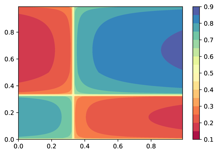
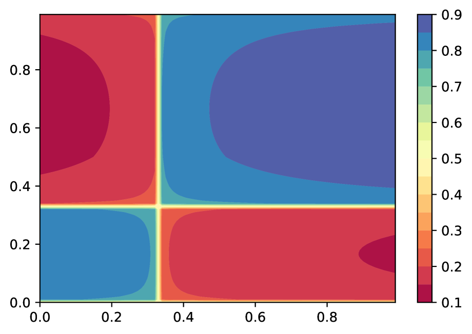
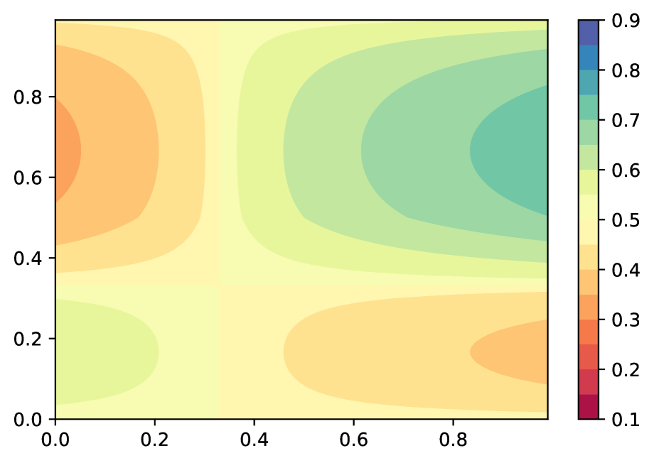
We consider the following pair of distributions and . The marginal distributions are both uniform distributions on . The regression function of is
while the regression function of with parameter is
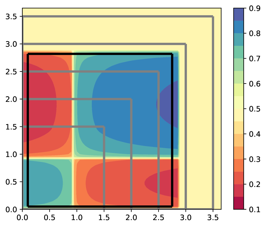
It can be easily verified that the constructed distributions above satisfy Assumption 3, 4, and 5. Throughout the following experiments, we take in 0.5 and 5. For better illustration, their regression functions are plotted in Figure 3.
We conduct experiments with privacy budgets . Here, can be regarded as the non-private case which marks the performance limitation of our methods. The other budget values cover all commonly seen magnitudes of privacy budgets. We take classification accuracy as the evaluation metric. In the simulation studies, the comparison methods and their abbreviation are as follows:
-
•
LPCT is the proposed algorithm with the max-edge partition rule. We select the parameters among and . We choose the Gini index as the reduction criterion.
-
•
LPCT-P and LPCT-Q are the estimation associated to and data, respectively. Their parameter grids are the same as LPCT-M.
-
•
LPCT-R is the proposed algorithm using the random max-edge partition [Cai+23]. Specifically, we randomly select an edge among the longest edges to cut at the midpoint. Its parameter grids are the same as LPCT-M.
- •
For each model, we report the best result over its parameter grids, with the best result determined based on the average result of at least 100 replications.
6.2 Simulation results
In Section 6.2.1 and 6.2.2, we analyze the influence of underlying parameters and sample sizes to validate the theoretical findings. In Section 6.2.3, we analyze the parameters of LPCT to understand their behaviors. We illustrate various ways that public data benefits the estimation in Section 6.2.4.
6.2.1 Influence of underlying parameters
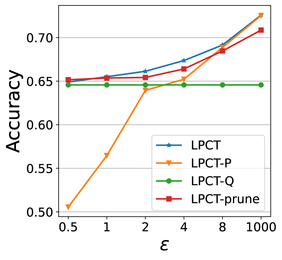
Privacy-utility trade-off
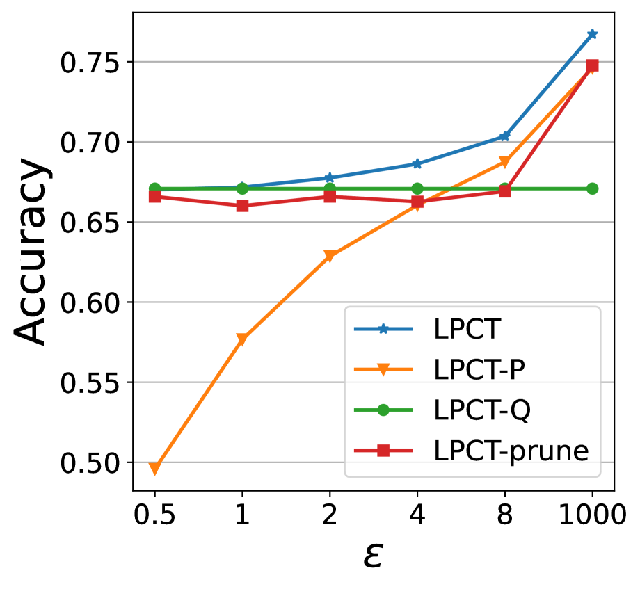
We analyze how the privacy budget influences the quality of prediction in terms of accuracy. We generate 10,000 private samples, with 50 and 1,000 public samples for and , respectively. The results are presented in Figure 4(a) and 4(b). In both cases, the performances of all models increase as increases. Furthermore, the performance of LPCT is consistently better than both LPCT-P and LPCT-Q, demonstrating the effectiveness of our proposed method in combining both data. LPCT-prune performs reasonably worse than LPCT. In the high privacy regime (), LPCT-P is almost non-informative and our estimator performs similarly to LPCT-Q. In the low privacy regime (), the performance of our estimator improves rapidly along with LPCT-P. In the medium regime, neither LPCT-P nor LPCT-Q obviously outperforms each other, and there is a clear performance gain from using LPCT.
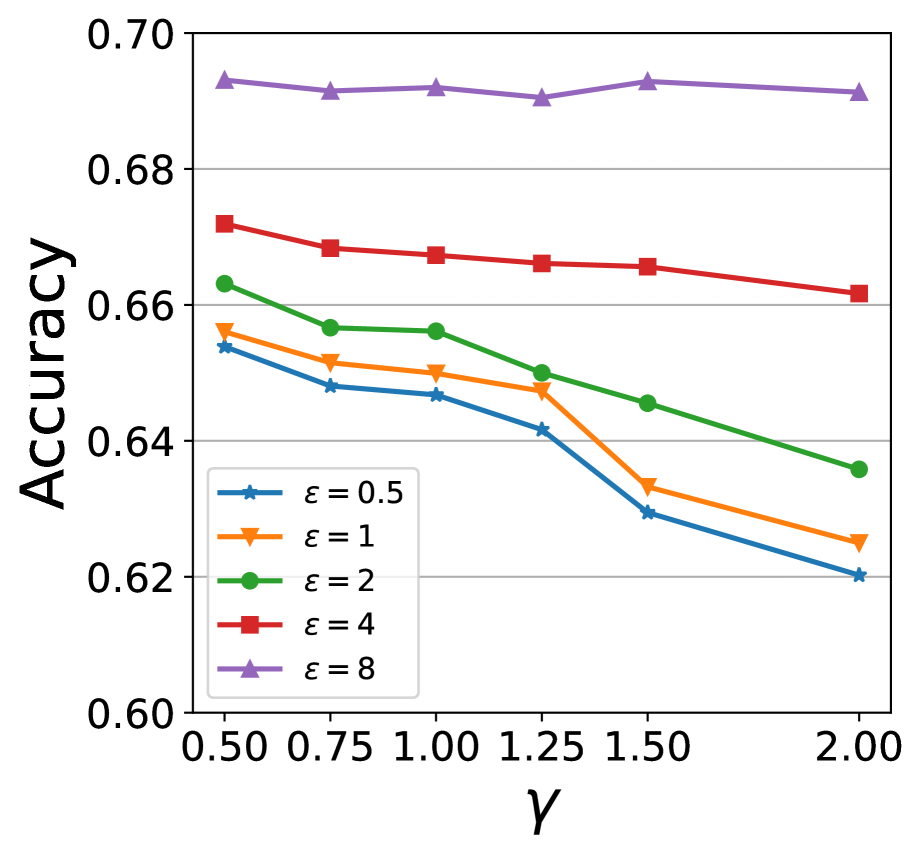
Influence of
We analyze how the relative signal exponent influences the performance. We set , and , while varying in . In Figure 4(c), we can see that the accuracy of LPCT is decreasing with respect to for all , which aligns with Theorem 7. Since only influences the performance through data, its effect is less apparent when the data takes the dominance, for instance .
6.2.2 Influence of sample sizes
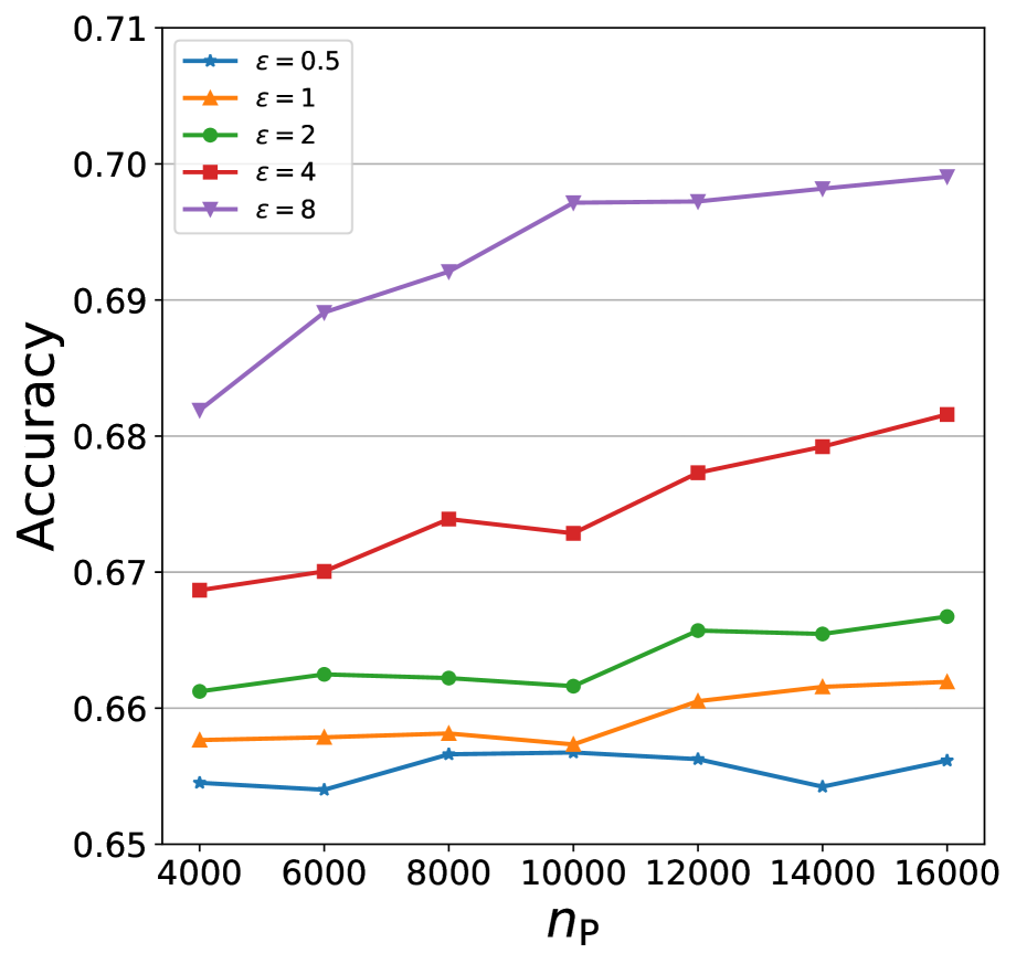
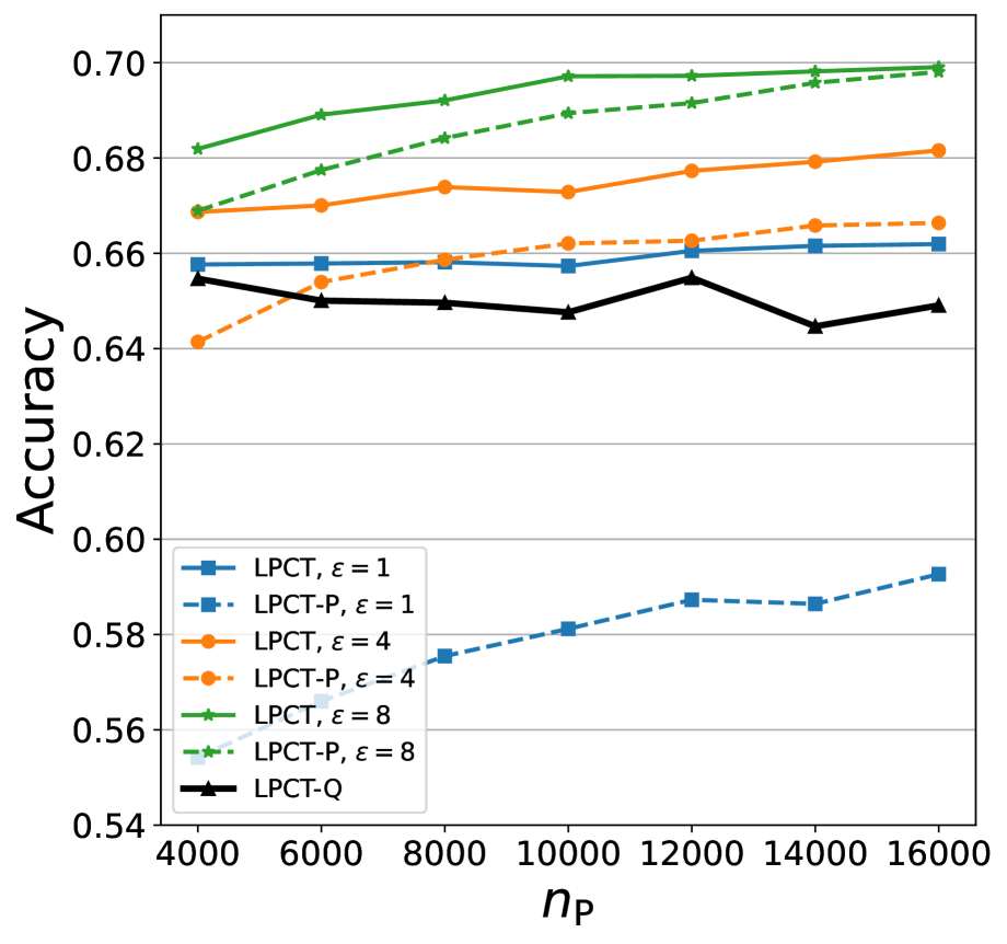
Accuracy -
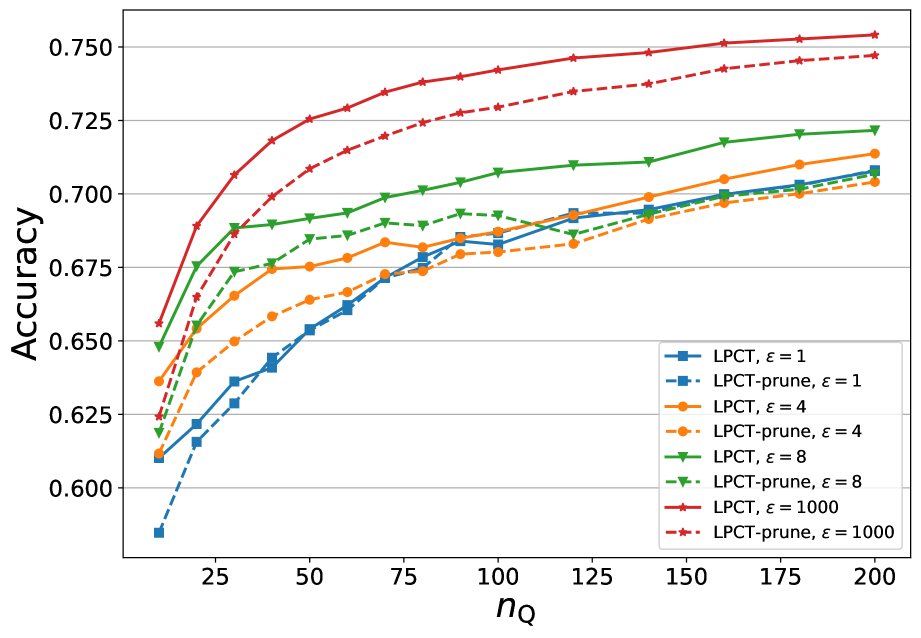
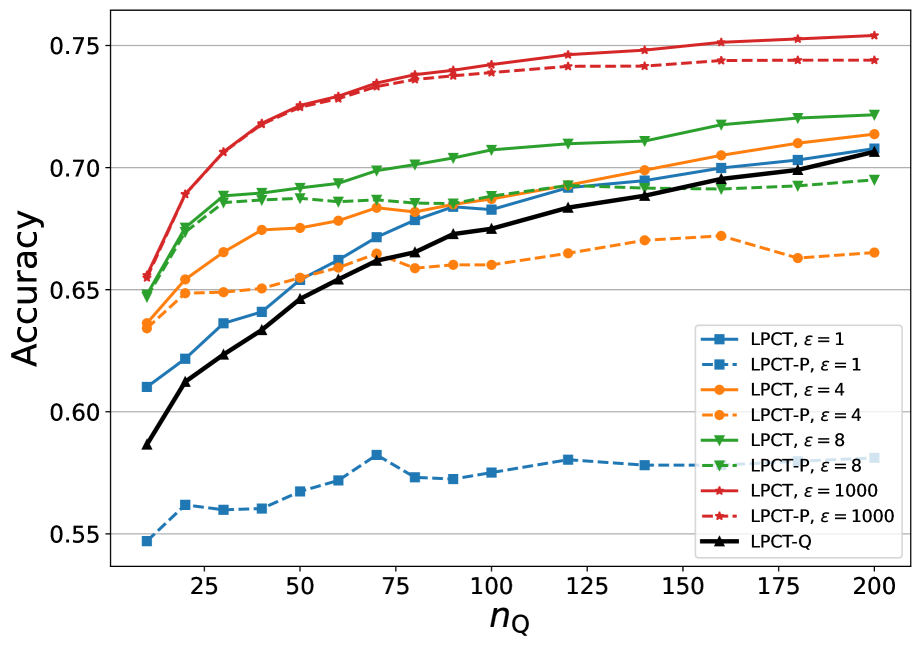
We conduct experiments to investigate the influence of the private sample size . We fix and while varying from to . The results are presented in Figure 5(a). Additionally, we compare the performance of LPCT-P and LPCT-Q to analyze the contribution of both datasets, as shown in Figure 5(b). Moreover, we compare LPCT and LPCT-prune in Figure 5(c). In Figure 5(a), except for , the accuracy improves as increases for all values. Moreover, the rate of improvement is more pronounced for higher values of . This observation aligns with the convergence rate established in Theorem 7. In 5(b), LPCT always outperforms methods using single datasets, i.e. LPCT-P and LPCT-Q. The improvement of LPCT over LPCT-Q is more significant for large . In Figure 5(c), we justify that LPCT-prune performs analogously to LPCT and its performance improves as and increase.
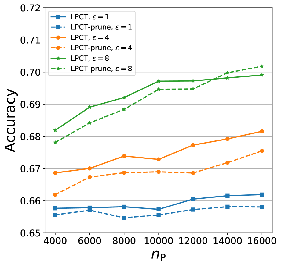
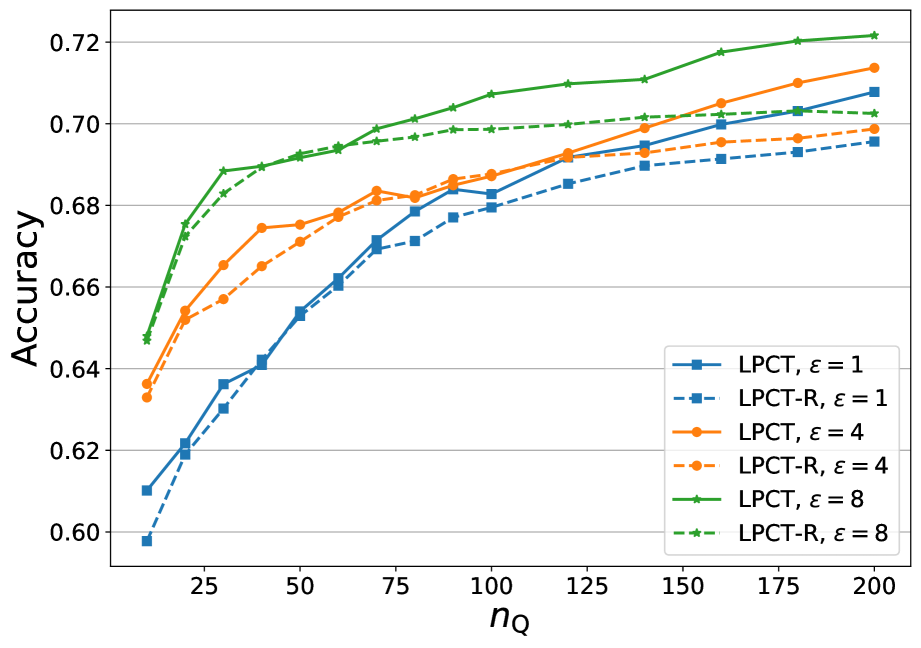
Accuracy -
We conduct experiments to investigate the influence of the private sample size . We keep and while varying from 10 to 200. The classification accuracy monotonically increases with respect to for all methods. In Figure 6(a), the performance of LPCT-prune is closer to LPCT when gets larger. As explained in Section 5.2, the pruning is appropriately conducted when data takes the dominance, and is disturbed when data takes the dominance. In Figure 6(b), it is worth noting that the performance improvement is more significant for small values of , specifically when . Moreover, the performance of LPCT-P also improves in this region and remains approximately unchanged for larger . This can be attributed to the information gained during partitioning, which is further validated in Figure 9.
6.2.3 Analysis of model parameters
Parameter analysis of depth
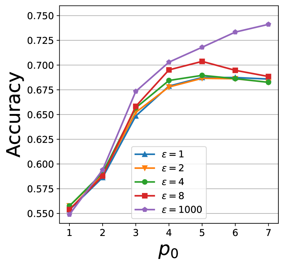
We conduct experiments to investigate the choice of depth. Under and , we plot the best performance of LPCT and LPCT-prune when fixing and to certain values, respectively in Figure 7(a) and 7(b). In Figure 7(a), the accuracy first increases as increases until it reaches a certain value. Then the accuracy begins to decrease as increases. This confirms the trade-off observed in Theorem 7. Moreover, the that maximizes the accuracy is increasing with respect to . This is compatible with the theory since the optimal choice is monotonically increasing with respect to . As in Figure 7(b), the accuracy increases with at first, whereas the performance remains unchanged or decreases slightly for larger than the optimum. Note that the axes of 7(a) and 7(b) are aligned. LPCT-prune behaves analogously to LPCT in terms of accuracy and optimal depth choice.
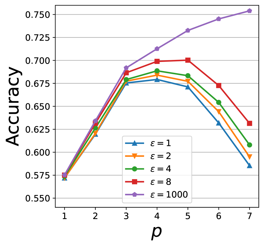
Parameter analysis of
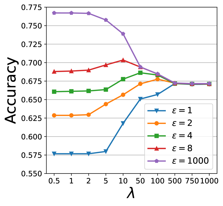
We conduct experiments to investigate the choice of in terms of accuracy. Under and , we plot in Figure 7(c) the best performance of LPCT when fixing to certain values. In Figure 7(c), the relation between accuracy and is inverted U-shaped for , while is monotonically increasing and decreasing for and , respectively. The results indicate that a properly chosen is necessary as stated in Theorem 7. Moreover, the that maximizes the accuracy is decreasing with respect to , which justify the fact that we should rely more on public data with higher privacy constraint.
6.2.4 Benefits of public data
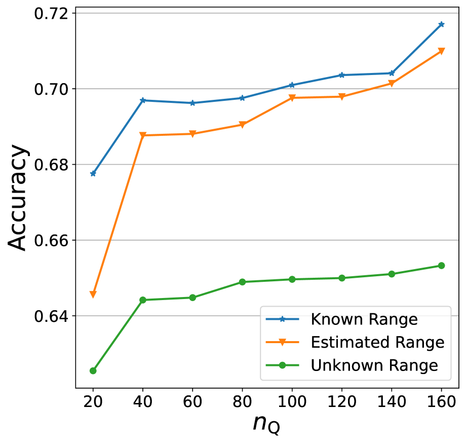
Range parameter
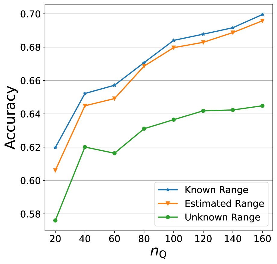
We demonstrate the effectiveness of range estimation using public data when the domain is unknown. Consider the case where and is a random variable uniformly distributed in . We compare the following scenarios: (I) is known. (II) is estimated using public data as shown in Theorem 8. (III) is unknown. Case (I) is equivalent to . In case (II), we min-max scale the samples from the estimated range to . In case (III), we scale the samples from to and select the best among . In Figure 8(a), we showcase the scaling schemes in (II) and (III). The estimated range from public data is much more concise than the best . Given no prior knowledge, the chosen in practice can perform significantly worse. In Figure 8(b) and 8(c), we observe that the performance of the estimated range matches that of (I) as increases, whereas the unknown range significantly degrades performance. The performance gap between the known and estimated range is more substantial when is small. This observation is compatible with the conclusion drawn in Theorem 8 emphasizing the need for sufficient public data to resolve the unknown range issue.
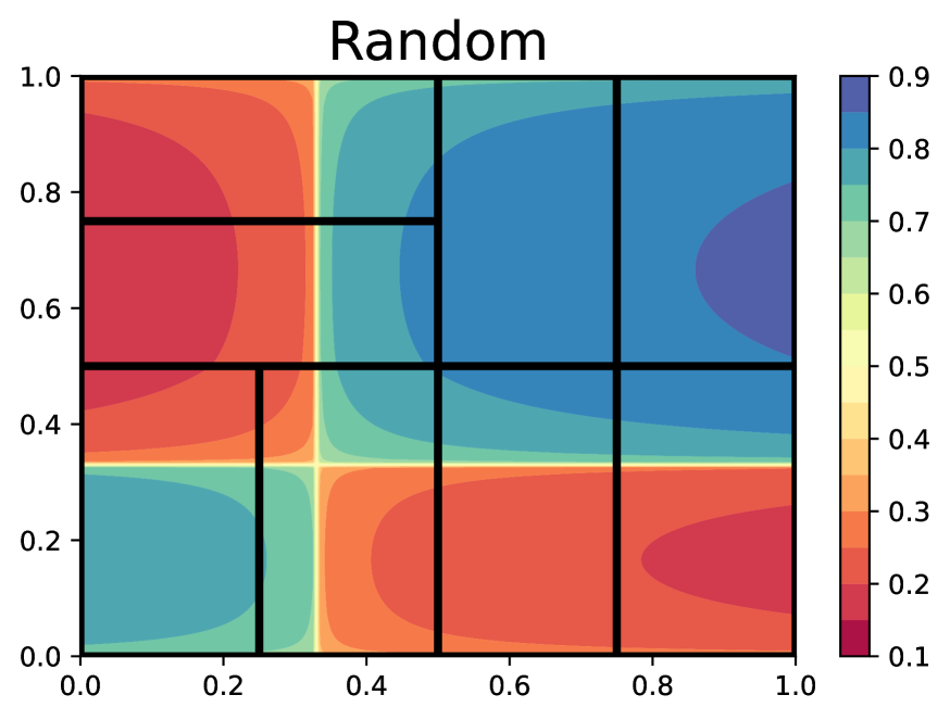
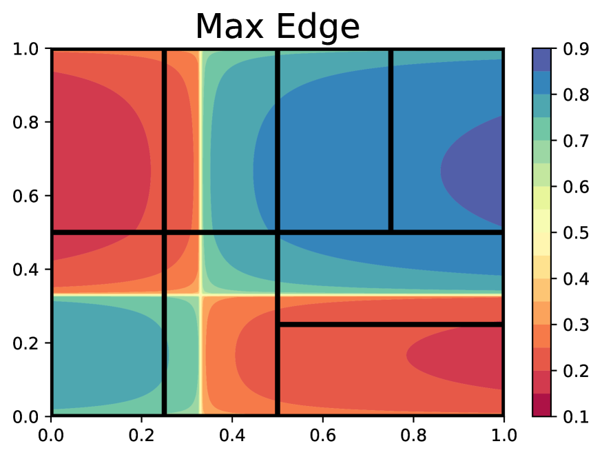
Partition
We demonstrate the effectiveness of partitioning with information of public data by comparing LPCT with LPCT-R. In Figure 9(a), the showcase of is presented. The random partition is possibly created as the top figure, where the upper left and the lower right cells are hard to distinguish as 0 or 1. Using sufficient public data, the max-edge partition is bound to create an informative partition like the lower figure. Moreover, Figure 9(b) shows that outperforms LPCT-R.
7 Experiments on real data
7.1 Data description
We conduct experiments on real-world data sets to show the superiority of LPCT in this section. We utilize 11 real datasets that are available online. Each of these datasets contains sensitive information and necessitates privacy protection. Furthermore, these datasets cover a wide range of sample sizes and feature dimensions commonly encountered in real-world scenarios. When creating and from the original dataset , some datasets have explicit criteria for splitting, reflecting real-world considerations. In these cases, we have . For others, the split is performed randomly and we have . A summary of key information for these datasets after pre-processing can be found in Table 1. Following the analysis in Section 4.3, we min-max scale each data to according to public data. Detailed data information and pre-processing procedures are provided in Appendix C.1.
| Dataset | d | Area | |||
|---|---|---|---|---|---|
| Anonymity | 453 | 50 | 14 | Social | |
| Diabetes | 2,054 | 200 | 8 | Medical | |
| 3,977 | 200 | 3,000 | Text | ||
| Employ | 2,225 | 200 | 8 | Business | |
| Rice | 240 | 3,510 | 7 | Image | |
| Census | 41,292 | 3,144 | 46 | Social | |
| Election | 1,752 | 222 | 9 | Social | |
| Employee | 3,319 | 504 | 9 | Business | |
| Jobs | 46,218 | 14,318 | 11 | Social | |
| Landcover | 7,097 | 131 | 28 | Image | |
| Taxi | 3,297,639 | 117,367 | 93 | Social |
7.2 Competitors
We compare LPCT with several state-of-the-art competitors. For each model, we report the best result over its parameter grids based on an average of 20 replications. The tested methods are
-
•
LPCT is described in Section 6. In real data experiments, we enlarge the grids to and due to the large sample size. Since the max-edge rule is easily affected by useless features or categorical features [Ma+23], we boost the performance of LPCT by incorporating the criterion reduction scheme from the original CART [Bre84] to the tree construction. Since Proposition 2 holds for any partition, the method is also -LDP. We choose the Gini index as the reduction criterion.
-
•
LPCT-prune is the same estimators described in Section 6. We also adopt the criterion reduction scheme for tree construction.
-
•
CT is the original classification tree [Bre84] with the same grid as LPCT. We define two approaches, CT-W and CT-Q. For CT-W, we fit CT on the whole data, namely and data together, with no privacy protection. Its accuracy will serve as an upper bound. For CT-Q, we fit CT on data only. Its performance is taken into comparison. We use implementation by sklearn [Ped+11] with default parameters while varying max_depth in .
-
•
PHIST is the locally differentially private histogram estimator proposed by [BB19]. We fit PHIST on private data solely as it does not leverage public data. We choose the number of splits along each axis in .
-
•
LPDT is the locally private decision tree originally proposed for regression [Ma+23]. The approach creates a partition on data and utilizes data for estimation. We adapt the strategy to classification. We select in the same range as LPCT.
-
•
PGLM is the locally private generalized linear model proposed by [Wan+23] with logistic link function. Note that their privacy result is under -LDP. We let for a fair comparison.
-
•
PSGD is the locally private stochastic gradient descent developed in [Low+23]. The presented algorithm is in a sequentially interactive manner, meaning that the privatized information from depends on the information from . We adopt the warm start paradigm where we first find a minimizer on the public data and then initialize the training process with the minimizer. Following [Low+23], we choose the parameters of the privacy mechanism, i.e. PrivUnitG, by the procedure they provided. We let and learning rate . We consider two models: PSGD-L is the linear classifier using the logistic loss; PSGD-N is the non-linear neural network classifier with one hidden layer and ReLU activation function. The number of neurons is selected in .
7.3 Experiment results
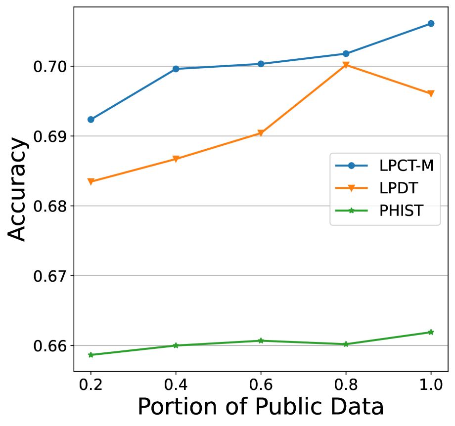
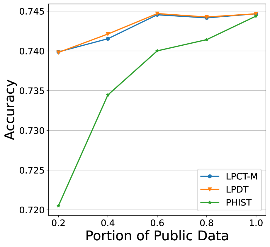
We first illustrate the substantial utility gain brought by public data. We choose Diabetes and Employee, representing the case of and , respectively. On each data, we randomly select a portion of private data and 80 public samples to train three models: LPCT, LPDT, and PHIST. PHIST does not leverage any information of public data, while LPDT benefits from public data only through the partition. LPCT utilizes public data in both partition and estimation. In Figure 10, the accuracy increases with respect to the extent of public data utilization for both identically and non-identically distributed public data. Moreover, the accuracy gain is significant. For instance, in Figure 10(b), 80 public samples and private samples achieve the same accuracy using private samples alone. The observation yields potential practical clues. For instance, when data-collecting resources are limited, organizations can put up rewards to get a small amount of public data rather than collecting a large amount of private data.
Next, we report the averaged accuracy for in Table 2 on each real data set. Here, CT-W is not private and serves as a reference. To ensure significance, we adopt the Wilcoxon signed-rank test [Wil92] with a significance level of 0.05 to check if the result is significantly better. For each dataset, trials that exceed a memory of 100GB or a running time of one hour are terminated.
| Datasets | CT-W | LPCT | LPCT-prune | CT-Q | PHIST | LPDT | PGLM | PSGD-L | PSGD-N | ||
| Maxedge | CART | Maxedge | CART | ||||||||
| Anonymity | 8.346 | 8.346* | 8.346* | 8.346* | 8.346* | 8.346* | 8.346* | 7.546 | 5.899 | 7.790 | 8.123 |
| Diabetes | 9.964 | 7.067 | 7.590* | 6.489 | 7.398 | 7.301 | 6.676 | 6.305 | 5.499 | 6.582 | 6.448 |
| 9.261 | 7.332 | 7.487 | 7.176 | 7.060 | 7.283 | - | 7.112 | 5.136 | 6.435 | 6.292 | |
| Employ | 9.048 | 7.403 | 8.646* | 5.941 | 5.963 | 8.577 | 5.704 | 5.644 | 4.874 | 5.742 | 5.595 |
| Rice | 8.992 | 9.039 | 9.183* | 8.983 | 9.183* | 9.117 | 5.467 | 6.583 | 4.886 | 8.517 | 8.142 |
| Census | 8.685 | 8.539 | 8.743* | 8.017 | 8.440 | 8.285 | - | 7.195 | 5.104 | 8.310 | 8.405 |
| Election | 6.408 | 5.610 | 5.846 | 5.268 | 5.846 | 5.958* | 5.060 | 5.089 | 4.948 | 5.207 | 5.074 |
| Employee | 7.648 | 7.397* | 7.131 | 6.383 | 6.777 | 7.151 | 6.660 | 6.098 | 5.280 | 6.493 | 6.387 |
| Jobs | 7.863 | 5.628 | 7.814* | 5.575 | 7.671 | 7.599 | 5.327 | 5.441 | 4.942 | 5.530 | 5.732 |
| Landcover | 9.404 | 8.615 | 8.960 | 8.249 | 8.504 | 6.670 | 8.362 | 8.366 | 4.955 | 8.368 | 8.349 |
| Taxi | 9.601 | 5.647 | 9.589* | 5.416 | 9.589* | 9.490 | - | 5.438 | 4.912 | - | - |
| Rank Sum | 35 | 21* | 64 | 35 | 36 | 81 | 82 | 106 | 66 | 79 | |
| No. 1 | 2 | 10* | 1 | 5 | 5 | 1 | 0 | 0 | 0 | 0 | |
| Datasets | CT-W | LPCT | LPCT-prune | CT-Q | PHIST | LPDT | PGLM | PSGD-L | PSGD-N | ||
| Maxedge | CART | Maxedge | CART | ||||||||
| Anonymity | 8.346 | 8.346* | 8.346* | 8.346* | 8.346* | 8.346* | 8.346* | 8.346* | 5.899 | 7.965 | 8.039 |
| Diabetes | 9.964 | 7.274 | 7.590* | 6.529 | 7.401 | 7.301 | 6.676 | 6.676 | 5.499 | 6.653 | 6.674 |
| 9.261 | 7.350 | 7.485* | 7.176 | 7.060 | 7.283 | - | 7.181 | 5.136 | 7.136 | 7.203 | |
| Employ | 9.048 | 7.702 | 9.121* | 5.966 | 5.962 | 8.577 | 6.174 | 7.181 | 4.874 | 5.786 | 5.792 |
| Rice | 8.992 | 9.027 | 9.183* | 8.983 | 9.183* | 9.117 | 5.467 | 8.458 | 4.886 | 9.050 | 8.750 |
| Census | 8.685 | 8.537 | 8.743* | 8.017 | 8.440 | 8.285 | - | 8.017 | 5.104 | 8.432 | 8.471 |
| Election | 6.408 | 5.648 | 5.850 | 5.268 | 5.846 | 5.958* | 5.056 | 5.114 | 4.948 | 5.323 | 5.111 |
| Employee | 7.648 | 7.437* | 7.175 | 6.383 | 6.777 | 7.151 | 6.472 | 6.951 | 5.280 | 6.400 | 6.383 |
| Jobs | 7.863 | 5.628 | 7.821* | 5.575 | 7.671 | 7.599 | 5.333 | 5.591 | 4.942 | 6.788 | 5.934 |
| Landcover | 9.404 | 8.715 | 8.960* | 8.249 | 8.504 | 6.670 | 8.367 | 8.493 | 4.955 | 8.553 | 8.369 |
| Taxi | 9.601 | 5.659 | 9.590* | 5.416 | 9.589 | 9.490 | - | 5.536 | 4.912 | - | - |
| Rank Sum | 37 | 20* | 73 | 42 | 37 | 80 | 67 | 103 | 70 | 76 | |
| No. 1 | 3 | 10* | 1 | 5 | 4 | 1 | 1 | 0 | 1 | 0 | |
| Datasets | CT-W | LPCT | LPCT-prune | CT-Q | PHIST | LPDT | PGLM | PSGD-L | PSGD-N | ||
| Maxedge | CART | Maxedge | CART | ||||||||
| Anonymity | 8.346 | 8.346* | 8.346* | 8.346* | 8.346* | 8.346* | 8.346* | 8.346* | 5.395 | 8.338 | 8.154 |
| Diabetes | 9.964 | 7.503 | 7.930* | 6.628 | 7.410 | 7.301 | 6.676 | 7.496 | 5.588 | 7.244 | 7.101 |
| 9.261 | 7.355 | 7.520 | 7.176 | 7.060 | 7.283 | - | 7.326 | 5.271 | 8.446 | 7.060 | |
| Employ | 9.048 | 7.619 | 9.068* | 5.921 | 5.961 | 8.577 | 9.043 | 7.572 | 5.237 | 5.795 | 5.798 |
| Rice | 8.992 | 9.011 | 9.183* | 8.983 | 9.181 | 9.117 | 8.858 | 9.017 | 6.283 | 9.017 | 8.875 |
| Census | 8.685 | 8.557 | 8.743* | 8.017 | 8.440 | 8.285 | - | 8.527 | 5.389 | 8.530 | 8.154 |
| Election | 6.408 | 5.894 | 6.082* | 5.368 | 5.846 | 5.958 | 5.015 | 5.892 | 5.462 | 5.765 | 5.705 |
| Employee | 7.648 | 7.441* | 7.173 | 6.383 | 6.777 | 7.151 | 7.437 | 7.439 | 4.930 | 6.775 | 6.883 |
| Jobs | 7.863 | 5.650 | 7.861* | 5.575 | 7.671 | 7.599 | 5.992 | 5.641 | 6.802 | 7.712 | 7.414 |
| Landcover | 9.404 | 8.737 | 8.963 | 8.366 | 8.504 | 6.670 | 8.367 | 8.695 | 5.551 | 9.137* | 8.948 |
| Taxi | 9.601 | 5.666 | 9.610* | 5.416 | 9.589 | 9.490 | - | 5.620 | 5.087 | - | - |
| Rank Sum | 39 | 22* | 77 | 43 | 39 | 83 | 64 | 104 | 56 | 78 | |
| No. 1 | 2 | 8* | 1 | 3 | 4 | 2 | 2 | 0 | 3 | 0 | |
From Table 2, we can see that LPCT-based methods generally outperform their competitors, both in the sense of average performance (rank sum) and best performance (number of No.1). Compared to LPCT, LPCT-prune performs reasonably worse due to its data-driven nature. In practice, however, all other methods require parameter tuning which limits the privacy budget for the final estimation. Thus, their real performance is expected to drop down while that of LPCT-prune remains. Methods with the CART rule substantially outperform those with the max-edge rule, as the CART rule is robust to useless features or categorical features and can fully employ data information. We note that on some datasets, the results of LPCT remain the same for all . This is the case where public data takes dominance and the estimator is barely affected by private data. Moreover, we observe that linear classifiers such as PSDG-L and PGLM perform poorly on some datasets. This is attributed to the non-linear underlying nature of these datasets.
We compare the efficiency of the methods by reporting the total running time in Table 3. PSGD-L and PSGD-N are generally slower and even take more than one hour for a single round on taxi data. Compared to these sequential-LDP methods, non-interactive methods achieve acceptable running time. We argue that the performance gap between LPCT and CT is caused by cython acceleration in sklearn. Moreover, PHIST causes memory leakage on three datasets. Though histogram-based methods and tree-based methods possess the same storage complexity theoretically [Ma+23], LPCT avoids memory leakage when is large in practice. The results show that LPCT is an efficient method.
| Datasets | CT-W | LPCT | LPCT-prune | CT-Q | PHIST | LPDT | PGLM | PSGD-L | PSGD-N | ||
|---|---|---|---|---|---|---|---|---|---|---|---|
| Maxedge | CART | Maxedge | CART | ||||||||
| Anonymity | 3e-3 | 1e-2 | 6e-3 | 9e-3 | 1e-2 | 2e-3 | 1e-2 | 2e-3 | 2e-3 | 8e-1 | 1e0 |
| Diabetes | 1e-2 | 1e-1 | 3e-2 | 3e-2 | 3e-2 | 3e-3 | 3e-2 | 6e-3 | 3e-3 | 3e0 | 6e0 |
| 3e0 | 1e0 | 3e-2 | 2e-1 | 1e0 | 6e-2 | - | 1e0 | 4e0 | 8e0 | 3e3 | |
| Employ | 5e-3 | 9e-2 | 2e-1 | 1e0 | 9e-1 | 3e-3 | 3e-2 | 4e-2 | 4e-3 | 5e0 | 7e0 |
| Rice | 1e-2 | 2e-2 | 1e-2 | 1e-2 | 2e-2 | 2e-2 | 5e-3 | 6e-3 | 8e-3 | 2e0 | 2e0 |
| Census | 6e-1 | 1e0 | 5e0 | 6e-1 | 9e-1 | 3e-1 | - | 2e-1 | 5e-2 | 2e1 | 3e1 |
| Election | 1e-2 | 6e-2 | 3e-2 | 3e-2 | 3e-2 | 3e-3 | 1e0 | 3e-2 | 3e-3 | 3e0 | 5e0 |
| Employee | 6e-3 | 8e-2 | 1e-1 | 4e-2 | 1e-1 | 3e-3 | 5e-2 | 5e-2 | 4e-3 | 7e0 | 1e2 |
| Jobs | 1e-1 | 1e0 | 1e0 | 6e-1 | 6e-1 | 3e-2 | 8e-1 | 5e-1 | 3e-2 | 1e2 | 1e2 |
| Landcover | 2e-1 | 1e-1 | 8e-2 | 9e-2 | 1e-1 | 5e-3 | 2e-1 | 9e-2 | 5e-3 | 1e1 | 2e1 |
| Taxi | 1e2 | 2e2 | 7e1 | 4e1 | 4e1 | 1e0 | - | 1e2 | 1e0 | - | - |
8 Conclusion and discussions
In this work, we address the under-explored problem of public data assisted LDP learning by investigating non-parametric classification under the posterior drift assumption. We propose the locally private classification tree that achieves the mini-max optimal convergence rate. Moreover, we introduce a data-driven pruning procedure that avoids parameter tuning and produces an estimator with a fast convergence rate. Extensive experiments on synthetic and real datasets validate the superior performance of these methods. Both theoretical and experimental results suggest that public data is significantly more effective compared to data under privacy protection. This finding leads to practical suggestions. For instance, prioritizing non-private data collection should be considered. When data-collecting resources are limited, organizations can offer rewards to encourage users to share non-private data instead of collecting a large amount of privatized data.
We summarize the ways that public data contributes to LPCT. The benefits lie in four-fold: (1) Elimination of range parameter. Since the domain is unknown in the absence of the raw data, the convergence rate and performance of partition-based estimators are degraded by a range parameter. For LPCT, public data helps to eliminate the range parameter both theoretically and empirically, as demonstrated in Section 4.3 and 6.2.4, respectively. (2) Implicit information in partition. Through the partition created on public data, LPCT implicitly feeds information from public data to the estimation. The performance gain is explained empirically in Section 6.2.4. (3) Augmented estimation. In the weighted average estimation, the public data reduces the instability caused by perturbations and produces more accurate estimations. Theoretically, the convergence rate can be significantly improved. Empirically, even a small amount of public data improves the performance significantly (Section 6 and 7). (4) Data-driven pruning. As shown in Section 5.2, we are capable of deriving the data-driven approach only with the existence of public data.
We discuss the potential future works and improvements. The assumption that and are identical can be mitigated. Similar to [Ma+23], we only need the density ratio to be bounded. Moreover, the marginal densities are not necessarily lower bounded, if we add a parameter to guarantee that sufficient samples are contained in each cell [Ma+23]. In practice, and can be distinctive [Yu+21a, GKW23]. This problem is related to domain adaption [Red+20] and can serve as future work direction. Determining whether a dataset satisfies Assumption 5 is of independent interest, as demonstrated in [GKW23, Yu+23].
References
- [Aba+16] Martin Abadi et al. “Deep learning with differential privacy” In Proceedings of the 2016 ACM SIGSAC conference on computer and communications security, 2016
- [ABM19] Noga Alon, Raef Bassily and Shay Moran “Limits of private learning with access to public data” In Advances in neural information processing systems 32, 2019
- [Ami+22] Ehsan Amid et al. “Public data-assisted mirror descent for private model training” In International Conference on Machine Learning, 2022 PMLR
- [AT07] Jean-Yves Audibert and Alexandre B Tsybakov “Fast learning rates for plug-in classifiers” In Annals of statistics 35.2, 2007, pp. 608–633
- [Bas+20] Raef Bassily et al. “Private query release assisted by public data” In International Conference on Machine Learning, 2020, pp. 695–703 PMLR
- [BB19] Thomas Berrett and Cristina Butucea “Classification under local differential privacy” In arXiv preprint arXiv:1912.04629, 2019
- [Ben+23] Shai Ben-David et al. “Private Distribution Learning with Public Data: The View from Sample Compression” In Advances in Neural Information Processing Systems Accepted, 2023
- [Ber46] Sergei N. Bernstein “The Theory of Probabilities” Gastehizdat Publishing House, Moscow, 1946
- [BGW21] Thomas B Berrett, László Györfi and Harro Walk “Strongly universally consistent nonparametric regression and classification with privatised data” In Electronic Journal of Statistics 15, 2021, pp. 2430–2453
- [Bis19] Balaka Biswas “Email Spam Classification Dataset CSV”, 2019 URL: https://www.kaggle.com/datasets/balaka18/email-spam-classification-dataset-csv/data
- [BK96] Barry Becker and Ronny Kohavi “Adult”, UCI Machine Learning Repository, 1996 URL: https://doi.org/10.24432/C5XW20
- [BKS22] Alex Bie, Gautam Kamath and Vikrant Singhal “Private Estimation with Public Data” In Advances in Neural Information Processing Systems, 2022
- [Bre84] L Breiman “Classification and Regression Trees” In The Wadsworth & Brooks/Cole Advanced Books & Software, 1984
- [BTG18] Raef Bassily, Om Thakkar and Abhradeep Guha Thakurta “Model-agnostic private learning” In Advances in Neural Information Processing Systems 31, 2018
- [BY21] Tom Berrett and Yi Yu “Locally private online change point detection” In Advances in Neural Information Processing Systems 34, 2021, pp. 3425–3437
- [Cai+23] Yuchao Cai, Yuheng Ma, Yiwei Dong and Hanfang Yang “Extrapolated Random Tree for Regression” In Proceedings of the 40th International Conference on Machine Learning PMLR, 2023, pp. 3442–3468
- [CCK14] Victor Chernozhukov, Denis Chetverikov and Kengo Kato “ANTI-CONCENTRATION AND HONEST, ADAPTIVE CONFIDENCE BANDS” In The Annals of Statistics 42.5, 2014, pp. 1787–1818
- [CD14] Kamalika Chaudhuri and Sanjoy Dasgupta “Rates of convergence for nearest neighbor classification” In Advances in Neural Information Processing Systems 27, 2014
- [CO19] Cammeo and Osmancik “Rice”, UCI Machine Learning Repository, 2019 URL: https://doi.org/10.24432/C5MW4Z
- [CV13] Kamalika Chaudhuri and Staal A Vinterbo “A stability-based validation procedure for differentially private machine learning” In Advances in Neural Information Processing Systems 26, 2013
- [CW21] T Tony Cai and Hongji Wei “Transfer learning for nonparametric classification: Minimax rate and adaptive classifier” In The Annals of Statistics 49.1, 2021
- [DF19] Amit Daniely and Vitaly Feldman “Locally private learning without interaction requires separation” In Advances in neural information processing systems 32, 2019
- [DF20] Yuval Dagan and Vitaly Feldman “Interaction is necessary for distributed learning with privacy or communication constraints” In Proceedings of the 52nd Annual ACM SIGACT Symposium on Theory of Computing, 2020, pp. 450–462
- [DG17] Dheeru Dua and Casey Graff “UCI Machine Learning Repository”, 2017 URL: http://archive.ics.uci.edu/ml
- [DJW13] John C Duchi, Michael I Jordan and Martin J Wainwright “Local privacy and statistical minimax rates” In 2013 IEEE 54th Annual Symposium on Foundations of Computer Science, 2013, pp. 429–438 IEEE
- [DJW18] John Duchi, Michael Jordan and Martin Wainwright “Minimax optimal procedures for locally private estimation” In Journal of the American Statistical Association 113.521 Taylor & Francis, 2018, pp. 182–201
- [Dri21] DrivenData “Differential Privacy Temporal Map Challenge: Sprint 3 (Prescreened Arena)”, 2021 URL: https://www.drivendata.org/competitions/77/deid2-sprint-3-prescreened/page/332/
- [Dwo+06] Cynthia Dwork, Frank McSherry, Kobbi Nissim and Adam Smith “Calibrating noise to sensitivity in private data analysis” In Theory of cryptography conference, 2006, pp. 265–284 Springer
- [Elm23] Tawfik Elmetwally “Employee dataset”, 2023 URL: https://www.kaggle.com/datasets/tawfikelmetwally/employee-dataset/data
- [EPK14] Úlfar Erlingsson, Vasyl Pihur and Aleksandra Korolova “Rappor: Randomized aggregatable privacy-preserving ordinal response” In Proceedings of the 2014 ACM SIGSAC conference on computer and communications security, 2014, pp. 1054–1067
- [Gan+23] Arun Ganesh et al. “Why Is Public Pretraining Necessary for Private Model Training?” In International Conference on Machine Learning, 2023, pp. 10611–10627 PMLR
- [GK22] László Györfi and Martin Kroll “On rate optimal private regression under local differential privacy” In arXiv preprint arXiv:2206.00114, 2022
- [GKW23] Xin Gu, Gautam Kamath and Zhiwei Steven Wu “Choosing Public Datasets for Private Machine Learning via Gradient Subspace Distance” In arXiv preprint arXiv:2303.01256, 2023
- [Ham22] Anas Hamoutn “Students’ Employability Dataset - Philippines”, 2022 URL: https://www.kaggle.com/datasets/anashamoutni/students-employability-dataset/data
- [JI16] Brian A Johnson and Kotaro Iizuka “Integrating OpenStreetMap crowdsourced data and Landsat time-series imagery for rapid land use/land cover (LULC) mapping: Case study of the Laguna de Bay area of the Philippines” In Applied Geography 67 Elsevier, 2016, pp. 140–149
- [Jos+19] Matthew Joseph, Janardhan Kulkarni, Jieming Mao and Steven Z Wu “Locally private gaussian estimation” In Advances in Neural Information Processing Systems 32, 2019
- [Kai+21] Peter Kairouz, Monica Ribero Diaz, Keith Rush and Abhradeep Thakurta “(Nearly) Dimension Independent Private ERM with AdaGrad Rates via Publicly Estimated Subspaces” In Conference on Learning Theory, 2021, pp. 2717–2746 PMLR
- [Kos08] Michael R. Kosorok “Introduction to Empirical Processes and Semiparametric Inference”, Springer Series in Statistics Springer, New York, 2008
- [KOV14] Peter Kairouz, Sewoong Oh and Pramod Viswanath “Extremal mechanisms for local differential privacy” In Advances in neural information processing systems 27, 2014
- [Lep92] OV Lepskii “Asymptotically minimax adaptive estimation. i: Upper bounds. optimally adaptive estimates” In Theory of Probability & Its Applications 36.4 SIAM, 1992, pp. 682–697
- [Li+22] Xuechen Li, Florian Tramèr, Percy Liang and Tatsunori Hashimoto “Large Language Models Can Be Strong Differentially Private Learners” In The Tenth International Conference on Learning Representations, 2022
- [Liu+21] Chong Liu, Yuqing Zhu, Kamalika Chaudhuri and Yu-Xiang Wang “Revisiting model-agnostic private learning: Faster rates and active learning” In The Journal of Machine Learning Research 22.1 JMLRORG, 2021, pp. 11936–11979
- [Low+23] Andrew Lowy, Zeman Li, Tianjian Huang and Meisam Razaviyayn “Optimal Differentially Private Learning with Public Data” In arXiv preprint arXiv:2306.15056, 2023
- [LT19] Jingcheng Liu and Kunal Talwar “Private selection from private candidates” In Proceedings of the 51st Annual ACM SIGACT Symposium on Theory of Computing, 2019
- [Ma+23] Yuheng Ma, Han Zhang, Yuchao Cai and Yang Hanfang “Decision Tree for Locally Private Estimation with Public Data” In Advances in Neural Information Processing Systems Accepted, 2023
- [Men+15] Aditya Menon, Brendan Van Rooyen, Cheng Soon Ong and Bob Williamson “Learning from corrupted binary labels via class-probability estimation” In International conference on machine learning, 2015, pp. 125–134 PMLR
- [Moh+22] Shubhankar Mohapatra et al. “The role of adaptive optimizers for honest private hyperparameter selection” In Proceedings of the aaai conference on artificial intelligence 36, 2022, pp. 7806–7813
- [MT07] Frank McSherry and Kunal Talwar “Mechanism design via differential privacy” In 48th Annual IEEE Symposium on Foundations of Computer Science (FOCS’07), 2007, pp. 94–103 IEEE
- [Nas+23] Milad Nasr et al. “Effectively Using Public Data in Privacy Preserving Machine Learning” In Proceedings of the 40th International Conference on Machine Learning 202 PMLR, 2023
- [Pap+17] Nicolas Papernot et al. “Semi-supervised Knowledge Transfer for Deep Learning from Private Training Data” In International Conference on Learning Representations, 2017
- [Pap+18] Nicolas Papernot et al. “Scalable Private Learning with PATE” In International Conference on Learning Representations, 2018
- [Ped+11] F. Pedregosa et al. “Scikit-learn: Machine Learning in Python” In Journal of Machine Learning Research 12, 2011, pp. 2825–2830
- [piA19] piAI “Internet Privacy Poll”, 2019 URL: https://www.kaggle.com/datasets/econdata/internet-privacy-poll
- [Por23] Nandita Pore “Healthcare Diabetes Dataset”, 2023 URL: https://www.kaggle.com/datasets/nanditapore/healthcare-diabetes/data
- [PS21] Nicolas Papernot and Thomas Steinke “Hyperparameter Tuning with Renyi Differential Privacy” In International Conference on Learning Representations, 2021
- [Ram+20] Swaroop Ramaswamy et al. “Training production language models without memorizing user data” In arXiv preprint arXiv:2009.10031, 2020
- [Red+20] Ievgen Redko et al. “A survey on domain adaptation theory: learning bounds and theoretical guarantees” In arXiv preprint arXiv:2004.11829, 2020
- [Sam12] Richard J Samworth “OPTIMAL WEIGHTED NEAREST NEIGHBOUR CLASSIFIERS” In The Annals of Statistics JSTOR, 2012, pp. 2733–2763
- [SCS13] Shuang Song, Kamalika Chaudhuri and Anand D Sarwate “Stochastic gradient descent with differentially private updates” In 2013 IEEE global conference on signal and information processing, 2013, pp. 245–248 IEEE
- [STU17] Adam Smith, Abhradeep Thakurta and Jalaj Upadhyay “Is interaction necessary for distributed private learning?” In 2017 IEEE Symposium on Security and Privacy (SP), 2017, pp. 58–77 IEEE
- [SXW23] Jinyan Su, Jinhui Xu and Di Wang “On PAC Learning Halfspaces in Non-interactive Local Privacy Model with Public Unlabeled Data” In Asian Conference on Machine Learning, 2023, pp. 927–941 PMLR
- [Tan+17] Jun Tang et al. “Privacy loss in apple’s implementation of differential privacy on macos 10.12” In arXiv preprint arXiv:1709.02753, 2017
- [Tan23] Ayush Tankha “Employability Classification of Over 70,000 Job Applicants”, 2023 URL: https://www.kaggle.com/datasets/ayushtankha/70k-job-applicants-data-human-resource/data
- [TKC22] Florian Tramèr, Gautam Kamath and Nicholas Carlini “Considerations for Differentially Private Learning with Large-Scale Public Pretraining” In arXiv preprint arXiv:2212.06470, 2022
- [Tsy09] Alexandre B. Tsybakov “Introduction to Nonparametric Estimation” Revised and extended from the 2004 French original, Translated by Vladimir Zaiats, Springer Series in Statistics Springer, New York, 2009, pp. xii+214 DOI: 10.1007/b13794
- [Wai19] Martin J Wainwright “High-dimensional statistics: A non-asymptotic viewpoint” Cambridge University Press, 2019
- [Wan+20] Di Wang, Marco Gaboardi, Adam Smith and Jinhui Xu “Empirical risk minimization in the non-interactive local model of differential privacy” In The Journal of Machine Learning Research 21.1 JMLRORG, 2020, pp. 8282–8320
- [Wan+23] Di Wang et al. “Generalized Linear Models in Non-interactive Local Differential Privacy with Public Data” In Journal of Machine Learning Research 24.132, 2023, pp. 1–57
- [Wan+23a] Hua Wang et al. “DP-HyPO: An Adaptive Private Framework for Hyperparameter Optimization” In Thirty-seventh Conference on Neural Information Processing Systems, 2023
- [War65] Stanley L Warner “Randomized response: A survey technique for eliminating evasive answer bias” In Journal of the American Statistical Association 60.309 Taylor & Francis, 1965, pp. 63–69
- [WGX18] Di Wang, Marco Gaboardi and Jinhui Xu “Empirical risk minimization in non-interactive local differential privacy revisited” In Advances in Neural Information Processing Systems 31, 2018
- [Wil92] Frank Wilcoxon “Individual comparisons by ranking methods” In Breakthroughs in statistics Springer, 1992, pp. 196–202
- [WSX19] Di Wang, Adam Smith and Jinhui Xu “Noninteractive locally private learning of linear models via polynomial approximations” In Algorithmic Learning Theory, 2019, pp. 898–903 PMLR
- [WT22] Larry Winner and Jared Thacker “1992 U.S Presidential Election”, 2022 URL: https://www.kaggle.com/datasets/jwt0024/1992-us-presidential-election
- [Wu+22] Xiaotong Wu et al. “An ensemble of random decision trees with local differential privacy in edge computing” In Neurocomputing 485 Elsevier, 2022, pp. 181–195
- [WX20] Di Wang and Jinhui Xu “Principal component analysis in the local differential privacy model” In Theoretical computer science 809 Elsevier, 2020, pp. 296–312
- [WZ20] Jun Wang and Zhi-Hua Zhou “Differentially private learning with small public data” In Proceedings of the AAAI Conference on Artificial Intelligence 34, 2020
- [Yu+21] Da Yu, Huishuai Zhang, Wei Chen and Tie-Yan Liu “Do not Let Privacy Overbill Utility: Gradient Embedding Perturbation for Private Learning” In International Conference on Learning Representations, 2021
- [Yu+21a] Da Yu et al. “Large scale private learning via low-rank reparametrization” In International Conference on Machine Learning, 2021, pp. 12208–12218 PMLR
- [Yu+22] Da Yu et al. “Differentially Private Fine-tuning of Language Models” In The Tenth International Conference on Learning Representations, 2022
- [Yu+23] Da Yu et al. “Selective Pre-training for Private Fine-tuning” In arXiv preprint arXiv:2305.13865, 2023
- [ZMW17] Kai Zheng, Wenlong Mou and Liwei Wang “Collect at once, use effectively: Making non-interactive locally private learning possible” In International Conference on Machine Learning, 2017, pp. 4130–4139 PMLR
- [ZWB21] Yingxue Zhou, Steven Wu and Arindam Banerjee “Bypassing the Ambient Dimension: Private SGD with Gradient Subspace Identification” In International Conference on Learning Representations, 2021
Appendix A Methodology
A.1 Estimator summarization
A.2 Derivation of the closed-form solution for pruning procedure
Remind that
For each and , define the quantity
Also, let . When the signs of and are identical, the object in (15) becomes
where the inequality follows from Cauthy’s inequality. The maximum is attained when
By bringing in , this leads to the solution
When and have different signs, the object in (15) is maximized at the extremum, i.e. when or . The maximum value is
Appendix B Proofs
B.1 Proof of Proposition 2
Proof of Proposition 2.
For each conditional distribution , we can compute the density ratio as
| (16) |
The first part is characterized by the Laplace mechanism. Since the conditional density is identical if and belongs to a same , we have
The right-hand side can be computed as
By definition, and are one-hot vectors and differ at most on two entries. As a result,
| (17) |
For the second part, note that and also differ at most on two entries. Then with analogous steps, we have
| (18) |
Bringing (17) and (18) into (16) yields the desired conclusion. ∎
B.2 Proof of Theorem 6
Proof of Theorem 6.
The proof is analogous to [CW21, Theorem 3.2 ]. We first construct two classes of distributions and for . We then combine the information inequality under privacy constraint [DJW18] and Assouad’s Lemma [Tsy09]. We first define two classes of distributions by construction. Define the useful quantity
| (19) |
where , , and are some universal constants. Let
be a grid of points in the unit cube. Denote as points in . Since , we are interested in which are balls with radius centered at . Let denote the points that aren’t in any of the balls. Define function on :
And define
where , are some universal constants. Define the hypercube of pairs by
with and defined as follows. For conditional density, we let
Let all have the same marginal distribution on , with density defined as follows:
where is an normalizing constant that makes well-defined. Similar to [CW21], with a proper choice of all constants, is a subset of that satisfies 5, 3, and 4. Then it suffices to show that
Let and denote the total variation distance and the Hellinger distance between measures, respectively. Let denote the hamming distance between ordered indices. Let and be two indices in such that , i.e. they differ at only one element and . We compute the total variation between the induced and . By Scheffe’s theorem [Tsy09], there holds
Since the marginal distributions for both measures are identical, we have
According to [CW21], we have
| (20) |
Let conditional distribution be any transformation on that is - local differentially private as defined in Definition 1. Denote by the random variable mapped compositionally through and . Therefore, for , there holds
| (21) |
For the first term in (21), combining [Tsy09, Lemma 2.4 ] and [DJW18, Corollary 3 ] yields
This together with (19) lead to
| (22) |
For the second term in (21), (20) implies
Again, bringing in (19) leads to
| (23) |
Bringing (22), (23) into (21), we have
as long as the constants are small enough such that . Let
Apply [Tsy09, Theorem 2.12 ], there holds
| (24) |
Next, we reduce the mini-max risk into this quantity. Since
for any estimator , we can reduce the excess risk as
This together with (24) yield
∎
B.3 Proof of Theorem 7
To prove Theorem 7, we rely on the following decomposition.
| (25) |
where we define
| (26) |
| (27) |
Correspondingly, we let and .
Loosely speaking, the first error term quantifies the degradation brought by adding noises to the estimator, which we call the privatized error. The second term corresponds to the expected estimation error brought by the randomness of the data, which we call the sample error. The last term is called signal strength, which quantifies the uncertainty of the population regression function. In general, we want the absolute value of the third term to be large, (i.e. the population regression function is sure about the label) while the first and the second terms to be small (i.e. the noise is small). In the proof of Theorem 7, we specify a region containing points with strong signal strength. We show that the first two terms are dominated by the signal strength on . The following three lemmas provide bounds for each of the three terms.
Lemma 12 (Bounding of Privatized Error).
Lemma 13 (Bounding of Sample Error).
Lemma 14 (Bounding of Signal Strength).
We also need the following technical lemma.
Lemma 15.
Suppose . If we let
then the following statements hold:
All proofs are provided in Section B.4.
Proof of Theorem 7.
Remind the definition in (28). Theorem 7 takes and . We prove the theorem by separately considering the region
for constant such that . In this case, suppose we have . Then it suffices to take .
For , we show that . Without loss of generality, let . By Lemma 12, 13, and 14 we have
| (29) |
with probability with respect to . We first compare the signal strength with the privatized error. From the conditions in Theorem 7, we have the fact that .
By bringing in the value of and applying Lemma 15 (the first conclusion) , there holds
Thus, for sufficiently large , we have
| (30) |
Analogously, we compare the signal strength with the sample error, which is
By bringing in the value of and applying Lemma 15 (the first conclusion) , there holds
Thus, for sufficiently large and , we have
| (31) |
Combined with (30) and (31), (29) yields , which indicates that for all .
B.4 Proofs of Lemmas in Section B.3
To prove lemmas in Section B.3, we first present several technical results. Their proof will be found in Section B.4
Lemma 16.
Suppose are independent sub-exponential random variables with parameters [Wai19, Definition 2.9]. Then there holds
for any . Moreover, a standard Laplace random variable is sub-exponential with parameters . A union bound argument yields that
Lemma 17.
Lemma 18.
Lemma 19.
Let be the partition generated by Algorithm 1 with depth . Then for any , there holds
Proof of Lemma 12.
We intend to bound
For each and any , the error can be decomposed as
For the first term in , we can apply Lemma 16 and 18 to get
with probability at least , where we used the fact that
Using Lemma 15 (the second and the third conclusions), we know that the second term is the dominating term, indicating that
Analogously, by Lemma 17, there holds
| (32) |
as well as
The last step is by Lemma 15 (the second and the third conclusions), knowing that is the dominating term. Combining these three pieces, there holds
| (33) |
For , (32) and Lemma 16 together yields
| (34) |
Proof of Lemma 13.
Proof of Lemma 14.
Without loss of generality, consider for any . By Assumption 5, we have
| (37) |
If Assumption 3 holds, for any , we have
where the second last and the last inequalities come from Lemma 19 and the definition of , respectively. For sufficiently large , we have for all , and thus (37) yields
which yields the desired result. Note that the factor comes from the lower bound of ratio . ∎
Proof of Lemma 15.
We prove the statement by discussing four cases depending on the value of , , and , , .
Case (): and . We prove the three conclusions by turn. The first conclusion follows from
For the second conclusion, let for some constant . Note that we have . By replacing all terms with equivalent order of , it suffices to prove
The left-hand side is dominated respectively by and
Here, the inequality is drawn by
Note that we omit the log factor since the polynomial part of the left-hand side is strictly dominated by the right-hand side, yielding that the conclusion holds with sufficiently large and . For the last statement, the same procedure yields that it suffices to show
which holds since .
Case (): and . Compared to case (), the value is is multiplied by a factor . Thus, the first conclusion holds since the value of the left-hand side increases. The third conclusion holds since the value of the left-hand side decreases. For the second conclusion, by replacing all terms with equivalent order of , it suffices to prove
For the left-hand side, the first term is dominated as . Since , we have . Thus, the second term of left-hand side is controlled by .
Case (): and . We now have . There holds
for sufficiently large , which implies the first conclusion. For the second conclusion, we want
The left-hand side is dominated by the term . Thus, the conclusion holds since there holds for all , and . For the last statement, the same procedure yields that it suffices to show
Thus, the conclusion holds since the following conditions hold:
Case (): and . Compared to case (), the value is is multiplied by a factor . Thus, the first conclusion holds since the value of the left-hand side increases. The third conclusion holds since the value of the left-hand side decreases. For the second conclusion, by replacing all terms with equivalent order of , it suffices to prove
We have and . ∎
B.5 Proofs of results in Section B.4
In the subsequent proof, we define the empirical measure given samples , where is the Dirac function. To conduct our analysis, we need to introduce the following fundamental descriptions of covering number which enables an approximation of an infinite set by finite subsets.
Definition 20 (Covering Number).
Let be a metric space and . For , the -covering number of is denoted as
where .
To prove Lemma 21, we need the following fundamental lemma concerning the VC dimension of random partitions in Section 3.2. To this end, let be fixed and be a partition of with the number of splits and denote the collection of all partitions .
Lemma 21.
Let be the collection of all cells in . For all , there exists a universal constant such that
Before we proceed, we list the well-known Bernstein’s inequality that will be used frequently in the proofs. Lemma 22 was introduced in [Ber46] and can be found in many statistical learning textbooks.
Lemma 22 (Bernstein’s inequality).
Let and be real numbers, and be an integer. Furthermore, let be independent random variables satisfying , , and for all . Then for all , we have
Proof of Lemma 17.
Since and share the same marginal distribution, it is equivalent to prove
holds with probability at least for . Let be the collection of all cells in . Applying Lemma 21 with , there exists an -net with
| (38) |
such that for any , there exist some such that
Since
we get
| (39) |
Consequently, by the definition of the covering number and the triangle inequality, for any , there holds
Therefore, we get
| (40) | ||||
| (41) |
For any fixed , let the random variable be defined by for and for . Then we have , , and . According to Assumption 3, there holds . Applying Bernstein’s inequality in Lemma 22, we obtain
with probability at least . Then the union bound together with the covering number estimate (38) implies that
with probability at least . Let and . Then for any , we have . Therefore, we have
with probability at least . This together with (40) yields that
We now compare to see which term is dominating. Apply Lemma 15 (the first conclusion), we have
When and ,
When and ,
When and , the derivation is the same as the last situation. When and ,
These derivations imply that the first term is dominating the upper bound, which implies the desired result. ∎
Proof of Lemma 18.
For notation simplicity, let for and for . Let for and for . Let . Let be the collection of all cells in . Then there exists an -net with bounded by (38) such that for any , (39) holds for some . Consequently, by the definition of the covering number and the triangle inequality, for any , there holds
| (42) |
where the last inequality follow from the condition .
For any fixed , let the random variable be defined by for and for . Then we have , , and . According to Assumption 3, there holds . Applying Bernstein’s inequality in Lemma 22, we obtain
with probability at least . Similar to the proof of Lemma 17, one can show that for any , there holds
with probability at least . This together with (42) yields that
This implies the desired result by analogous derivations as in the last part of the proof of Lemma 17. ∎
Proof of Lemma 19.
According to the max-edge partition rule, when the depth of the tree is a multiple of dimension , each cell of the tree partition is a high-dimensional cube with a side length . On the other hand, when the depth of the tree is not a multiple of dimension , we consider the max-edge tree partition with depth and , whose corresponding side length of the higher dimensional cube is and . Note that in the splitting procedure of max-edge partition, the side length of each sub-rectangle decreases monotonically with the increase of , so the side length of a random tree partition cell is between and . This implies that
Since , we immediately get . ∎
B.6 Proof of Theorem 8
B.7 Proof of Proposition 9
Proof of Proposition 9.
We prove the conclusion for first. When and , the term can be written as
We bound the three parts separately. By Lemma 16, is bounded by
| (43) |
with probability for all . The proofs for and are analogous to the proof of Lemma 18 which utilizes Bernstein’s inequality with the VC dimension of possible squares on . is an independent sum of Bernoulli random variables with only non-zero elements. Thus by Bernstein’s inequality (Lemma 22), we have
with probability at least . The order of yields that . Since there are at most cells in the union of all , there holds
| (44) | ||||
with probability at least . By Lemma 16, for all , with probability , we have
If , there holds
as well as
for sufficiently large . In this case, we have
| (45) |
If , there holds
for sufficiently large . In this case, we get
| (46) |
Combinging (45) and (46), we get
| (47) |
Similarly to (44), we have
| (48) | ||||
with probability at least . Combining (47) and (48), we get
with probability at least . Here, we define constant for notation simplicity
We now prove the conclusion for with a slight modification on the above statement. For the term , summing among all nodes with the same ancestor yields the sum of Laplace random variables, for which we have
The proof is completed by bringing the bound into the decomposition in the beginning. ∎
B.8 Proof of Proposition 10
Lemma 23.
Suppose are independent standard exponential random variables. Then there holds
Moreover, a union-bound argument yields that
Proof of Lemma 23.
The conclusion follows directly from the central limit theorem and union-bound argument. ∎
Proof of Proposition 10.
Since we assumed that , we omit the effect of data in the following analysis, which causes only constant differences. We first show that (14) holds with a constant probability. The derivation in Section A.2 shows that
| (49) |
If , there holds
due to Lemma 17. By Lemma 23, this leads to
for sufficiently large with probability . As a result, the term is of the same order of , i.e.
| (50) |
Moreover, the definition of yields that , which indicates that the same conclusion holds for :
| (51) |
(50) and (51) together yield that both numerator and denominator of the estimation is dominated by the noises. Since both and are sums of independent exponential random variables, they are approximately distributed as standard normal. Thus, is approximately distributed as Cauchy distribution. As a result, there exist constants and such that
Bringing this into (49) yields
where is the cumulative distribution function of standard Gaussian distribution. Here, the second inequality comes from (50). The last inequality comes from first bringing in the definition of and then applying the central limit theorem.
To show the opposite direction, i.e. (14) does not hold, we first notice that if , an analysis analogous to above will yield
| (52) |
By (50) and definition of , this leads to
where is the cumulative distribution function of standard Gaussian distribution. Here, the second inequality comes from the central limit theorem. As for any order of , the probabilities and are determined is larger than a positive constant for all , the proof is completed. The positive constant depends only on and , where and depend only on the property of the standard Cauchy distribution.
Given the fact that (14) holds with a constant probability, to prove the proposition, we only consider the case where holds with a positive probability . If with high probability, then for sufficiently large , the first case holds any . Given this, we calculate the two probabilities under each and show that at least one of the statements holds. For notation simplicity, we denote
As a result, there exists constant such that . Then we have
for sufficiently large . For the second probability, there holds
For any large enough, there holds for some constant . As a result,
Then for any order of , which depends on , at least one of or is independent of and . Thus, we showed that at least one of and will happen.
∎
B.9 Proof of Theorem 11
In the proof, depth , , are all integers. Without loss of generality, we only write , , equal some order which will only cause difference in constants.
Proof of Theorem 11.
In the following proof, we give several version of upper bounds of for each fixed . Then, we consider the region which is
For some , by techniques analogous to the proof of Theorem 7, we can show that all in is assigned to the same label as the Bayes classifier. For each fixed , let denote the partition cell in that contains . We will discuss the stopping time of the pruning process and the resulting point-wise error. We prove the conclusion under two cases respectively.
Case (i): . Without loss of generality, we let . Following the analysis in Section A.2, the final statistics will satisfy
By Proposition 9, there exists a constant such that
| (53) |
with probability . Consider the region
Let . For each , by Lemma 14, there exist , such that,
| (54) |
Also, by Lemma 17, there exists constant such that
| (55) |
(54) and (55) together lead to
| (56) |
For sufficiently large constant , (56) yields that the choice of leads to
| (57) |
Combining (53) and (57), there holds the following
for the choice of . Thus, for and , the terminating condition will be triggered at least at , indicating that . Thus, in this case, we have
which implies that the signs of and are identical. By steps analogous to proof of Proposition 14, there holds for . Thus we show that, for each and , the label is assigned correctly as the Bayes classifier. Therefore, by Assumption 4, we have
Case (ii) . Under this case, the termination happens possibly at . The resulted estimator has a larger point-wise signal strength and thus can not be worse than the case where . Thus, in the following, we bound the excess risk of the estimator where for all .
Analogous to the proof of Lemma 12, there holds
| (58) |
Since , we have
Then (58) becomes
The noise on the numerator in each is , which is an independent sum of Laplace random variables. Applying Lemma 16 and 17, there holds
Since the estimation is based on now, the signal strength is bounded by
Then by the same logic in Case (i), the excess risk is bounded by
∎
Appendix C Experiment details
C.1 Real datasets pre-processing
We present additional information on the data sets including data source and pre-processing details. The datasets are sourced from UCI Machine Learning Repository [DG17] and Kaggle.
Anonymity: The Anonymity dataset [piA19] contains poll results about Internet privacy from a large number of people, including answers about whether the interviewee believes United States law provides reasonable privacy protection for Internet users or their conservativeness about Internet privacy. We use other variables to predict whether the interviewee has ever tried to mask his/her identity when using the Internet. We randomly select 50 samples as the public data.
Diabetes: This dataset from [Por23] contains a diverse range of health-related attributes, meticulously collected to aid in the development of predictive models for identifying individuals at risk of diabetes. We randomly select 200 samples as the public data.
Email: The dataset is used for spam or not-spam classification [Bis19]. For each row, the count of each word (column) in that email (row) is stored in the respective cells. Thus, information regarding all emails is stored in a compact data frame. We randomly select 200 samples as the public data.
Employ: The dataset [Ham22] was collected from different agencies in the Philippines consisting of mock interview performances of students. The final task is to decide whether the student got employed. We randomly select 200 samples as the public data.
Rice: The Rice dataset [CO19] contains morphological features obtained for two grains of rice to classify them. We randomly select 300 samples as the public data.
Census: This dataset is the well-known census data [BK96] and is used to predict whether income exceeds 50,000 per year. We select the samples whose native country is the U.S. to be public data and others to be private data.
Election: This dataset from [WT22] contains county-level demographics and whether or not Bill Clinton won each county during the 1992 U.S. presidential election. The goal of this dataset is to predict if Clinton won a county. We use samples whose state is TX as public data and the rest as private data.
Employee: The Employee data [Elm23] contains information about employees in a company, including their educational backgrounds, work history, and employment-related factors. We use these variables to predict whether the employee leaves or not. We select the sample to be public if the employee joined the company before 2012.
Jobs: The data [Tan23]contains a comprehensive collection of information regarding job applicants and their respective employability scores to predict whether the applicant has been hired. We select the samples whose native country is the U.S. to be public data and others to be private data.
Landcover: The data is from [JI16], which contains Landsat time-series satellite imagery information on given pixels and their corresponding land cover class labels (farm, forest, water, etc.) obtained from multiple sources. We classify whether the image comes from a farm or a forest. Within this dataset, there are two kinds of label sources: labels obtained from Open-StreetMap and labels that are accurately labeled by experts. We take the latter as public data and the former as private data.
Taxi: The Taxi dataset was obtained from the Differential Privacy Temporal Map Challenge [Dri21], which aims to develop algorithms that preserve data utility while guaranteeing individual privacy protection. The dataset contains quantitative and categorical information about taxi trips in Chicago, including time, distance, location, payment, and service provider. These features include the identification number of taxis (), time of each trip (), the distance of each trip (), index of the zone where the trip starts (), index of the zone where the trip ends (), service provider (), the method used to pay for the trip (), amount of tips () and fares (). We use the other variable to predict whether the passenger is paying by credit card or by cash. We select data from one company as public data and others as private data.