Coverage-Validity-Aware Algorithmic Recourse

Abstract.

Algorithmic recourse emerges as a prominent technique to promote the explainability, transparency and hence ethics of machine learning models. Existing algorithmic recourse approaches often assume an invariant predictive model; however, the predictive model is usually updated upon the arrival of new data. Thus, a recourse that is valid respective to the present model may become invalid for the future model. To resolve this issue, we propose a novel framework to generate a model-agnostic recourse that exhibits robustness to model shifts. Our framework first builds a coverage-validity-aware linear surrogate of the nonlinear (black-box) model; then, the recourse is generated with respect to the linear surrogate. We establish a theoretical connection between our coverage-validity-aware linear surrogate and the minimax probability machines (MPM). We then prove that by prescribing different covariance robustness, the proposed framework recovers popular regularizations for MPM, including the $\ell_{2}$-regularization and class-reweighting. Furthermore, we show that our surrogate pushes the approximate hyperplane intuitively, facilitating not only robust but also interpretable recourses. The numerical results demonstrate the usefulness and robustness of our framework.

1. Introduction

The recent prevalence of machine learning (ML) in the automation of consequential decisions related humans, such as loan approval [37], job hiring [12, 54], and criminal justice [10], urges the need of transparent ML systems with explanations and feedback to users [15, 36]. Algorithmic recourse [62] is an emerging approach for generating feedback in ML systems. A recourse suggests how the input instance should be modified in order to alter the outcome of a predictive model. Consider a specific scenario in which a financial institution’s ML model rejects the loan application of an individual. It has now become a legal necessity to provide explanations and recommendations to individuals to improve their situation and obtain a loan in the future (GDPR, [66]). For example, the recommendation can be “increase the income to $5000” or “reduce the debt/asset ratio to below 20%”. These recommendations empower individuals to understand the factors influencing their loan applications and take specific actions to address them. It also promotes transparency and fairness in the decision-making process, incentivizing users to improve their eligibility for loans.

Various techniques were proposed to devise algorithmic recourses for a given predictive model; extensive surveys are provided in [26, 59, 46, 63]. [68] introduced the definition of counterfactual explanations and proposed a gradient-based approach to finding the nearest instance that yields a favorable outcome. [62] proposed a mixed integer programming formulation (AR) that can find recourses for a linear classifier with a flexible design of the actionability constraints. In [27, 28], recourses that can accommodate causal relationships between features are investigated through the lens of minimal intervention. Recent works, including [52] and [38], studied the problem of generating a menu of diverse recourses to provide multiple possibilities that users might choose.

While these methods offer actionable recourses with low implementation costs, they face a critical downside regarding robustness in a real-world deployment. The recourse literature identifies three main types of robustness that are desirable: (i) robustness to changes in the input data point, which ensures consistent and comparable solutions for users with similar characteristics or needs [56], (ii) robustness to changes in attained recourses, which requires that the recommended actions to be stable with respect to minor variations in implementation [48, 35, 14, 64], (iii) robustness to model shifts, which are often caused by model retraining and updating [23, 71, 22, 41, 47, 8, 61].

Motivated by the fact that ML models are frequently retrained or recalibrated upon the arrival of new data, this paper focuses on the robustness with respect to model shifts. Because of the model shift, a recourse deemed valid for the current model may become invalid for the future model. For example, a second-time loan applicant, who has been rejected in his first attempt and spent great effort to achieve the recourse suggested by the ML system, could still be rejected (again), simply because of model shifts; see Figure 1 for an illustration. Such unfortunate events can result in inefficiency of the overall ML system, waste of resource and effort of the user, and distrust in ML systems in our society [51].

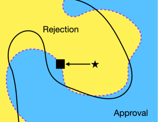
Figure 1. An example of recourse failures under model shifts. The present model’s boundary is plotted in a dashed curve, separating the input space into the rejection (yellow) and approval (blue) regions. The original input (star) lies in the rejection region of the present model. The recommended recourse (square symbol) is in the approval region of the present model. However, as the boundary shifts to the solid line, the recourse falls into the rejection region under the new boundary.

Studying this phenomenon, [49] first described several types of model shifts related to the correction, temporal, and geospatial shifts from data. They pointed out that even recourses constructed with state-of-the-art algorithms can be vulnerable to shifts in the model’s parameters. [47] studied counterfactual explanations under predictive multiplicity and its relation to the difference in how two classifiers treat predicted individuals. [8] showed that the constructed recourses might be invalid even for the model retrained with different initial conditions, such as weight initialization and leave-one-out variations in data.

To generate recourses that are robust to model shifts, [61] leveraged robust optimization to propose ROAR - wherein the parameter shifts are captured by an uncertainty set centered around the current parameter value of a linear surrogate. Methods using distributionally robust optimization have also been proposed, which capture the shifts of the parameters using probability distributions [11, 40]. This line of research formulates the design of recourse as a min-max problem, and the goal is to find a recourse that minimizes the loss function associated with the worst model parameters over the pre-specified range. Herein, the loss function can be an aggregation of different terms representing the implementation cost and the validity of the solution, among others. The min-max approach to recourse design is usually criticized for its over-conservativeness. In particular, whichever recourse is chosen, the corresponding worst shift parameter will be realized. As a consequence, although the min-max formulation can deliver a recourse with high validity, the cost for implementing the recourse is unrealistically high. Furthermore, compared with minimization or maximization problems, min-max problems are a more difficult class of computational problems. Not only the algorithmic design and analysis are much more involved, the computational complexity and ease of implementation are also worse than minimization/maximization problems in general. Finally, one may want to impose additional constraints to a mathematical formulation of the recourse design problem, for fairness, explainability or any other practical, legal or ethical considerations. These constraints are sometimes of mixed-integer type. Unfortunately, it is highly nontrivial to extend existing theory and algorithms of min-max formulations of the recourse design problem so as to allow extra constraints, especially ones involving integer variables.

These aforementioned methods all share the linear classifier setting, which is also a popular choice employed by earlier work on algorithmic recourse [62, 52, 49]. For non-linear classifiers, a linear surrogate method is used in the preprocessing step to locally approximate the nonlinear decision boundary of the black-box classifiers. The recourse is then generated subject to the linear surrogate instead of the nonlinear model. The most popular choice to construct the surrogate is Local Interpretable Model-Agnostic Explanations (LIME, [50]), a well-known method to explain ML predictions by fitting a reweighted linear regression model to the perturbed samples around an input instance. Arguably, LIME is the most common linear surrogate for the nonlinear decision boundary of the black-box models [62, 61]. Unfortunately, the LIME surrogate might not be locally faithful to the underlying model due to its weighted sampling scheme [32, 69]. Furthermore, it is also well-known that perturbation-based surrogates are sensitive to the original input and perturbations [2, 19, 58, 57, 1, 32]. Several approaches are proposed to overcome these limitations. [32] and [65] proposed alternative sampling procedures that generate sample instances in the neighborhood of the closest counterfactual to fit a local surrogate. [69] integrated counterfactual explanation to local surrogate models to introduce a novel fidelity measure of an explanation. Later, [17] and [1] analyzed theoretically the sensitivity of LIME, especially in the low sampling size regime. [72] leveraged Bayesian reasoning to improve the consistency in repeated explanations of a single prediction. However, the influence and efficacy of these surrogate models on the generation of recourse options remain elusive, especially when the situation is further complicated by model shifts.

1.1. Robust Surrogates for Actionable Recourse Generation

We propose a new framework for robust actionable recourse design: the core ingredient of our framework is the linear surrogate, which is known to be robust to the model shifts. The upshot is that our robust recourse generation framework does not need to solve a min-max problem. Hence, our method does not suffer from over-conservatism nor unfavorable complexity/scalability as in the (distributionally) robust recourse formulations. Moreover, it is amenable to additional constraints, even mix-integer ones, which allow us to impose fairness, legal, causality, explainability, ethical, or any other constraints easily.

To introduce our method, we assume that the covariate space is $\mathcal{X}=\mathbb{R}^{d}$, and we have a binary label space $\mathcal{Y}=\{-1,+1\}$. Without any loss of generality, we assume that label $-1$ encodes the unfavorable decision, while $+1$ encodes the favorable one. Given a black-box ML classifier $f$ and input $x_{0}$ with an unfavorable predicted outcome, we aim to find an actionable recourse recommendation for $x_{0}$ that has a high probability of being classified into a favorable group, subject to possible shifts of the ML classifier $f$. Such recourse is termed a robust actionable recourse. Figure 2 provides a schematic view of ur recourse generator consisting of three components:

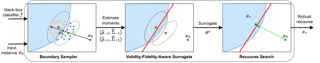
Figure 2. The sampler synthesizes new instances around $x_{0}$ and queries the predicted labels from the classifier $f$ . The moment information $(\widehat{\mu}_{y},\widehat{\Sigma}_{y})$ estimated from the synthetic pseudo-labeled data (represented by triangles and ellipsoids) serves as inputs to find the (covariance-robust) Coverage-Validity-Aware Surrogate. The surrogate $\theta^{\varphi}$ (red hyperplane) is the target classifier to generate recourses (red circle).

1. a local sampler: given an instance $x_{0}$, we choose $k$ nearest counterfactuals $x_{1},\ldots,x_{k}$ from the training data with the opposite predicted label to $x_{0}$. For each $x_{i}$, we perform a line search to find a point $x_{b,i}$ that is on the decision boundary and the line segment between $x_{0}$ and $x_{i}$. Among $x_{b,i}$, we choose the nearest point $x_{b}$ to $x_{0}$ and sample uniformly in an $\ell_{2}$-neighborhood with radius $r_{p}$ around $x_{b}$. We then query the black-box ML classifier $f$ to obtain the predicted labels of the synthetic samples.

2. a linear surrogate that explicitly balances the coverage-validity trade-off: we propose two performance metrics for the surrogate, coverage and validity, that are motivated by the popular precision-recall metrics in the machine learning literature. We then use the synthesized samples to estimate the moment information $(\widehat{\mu}_{y},\widehat{\Sigma}_{y})$ of the covariate conditional on each predicted class $y$, and then train a coverage-validity-aware linear surrogate to approximate the local decision boundary of the ML model.

3. a recourse search: in principle, we can integrate our coverage-validity-aware surrogate with any robust recourse search method to find a robust recourse. This paper uses two simplest recourse search methods: a simple projection and AR [62], a MIP-based framework, to promote actionable recourses.

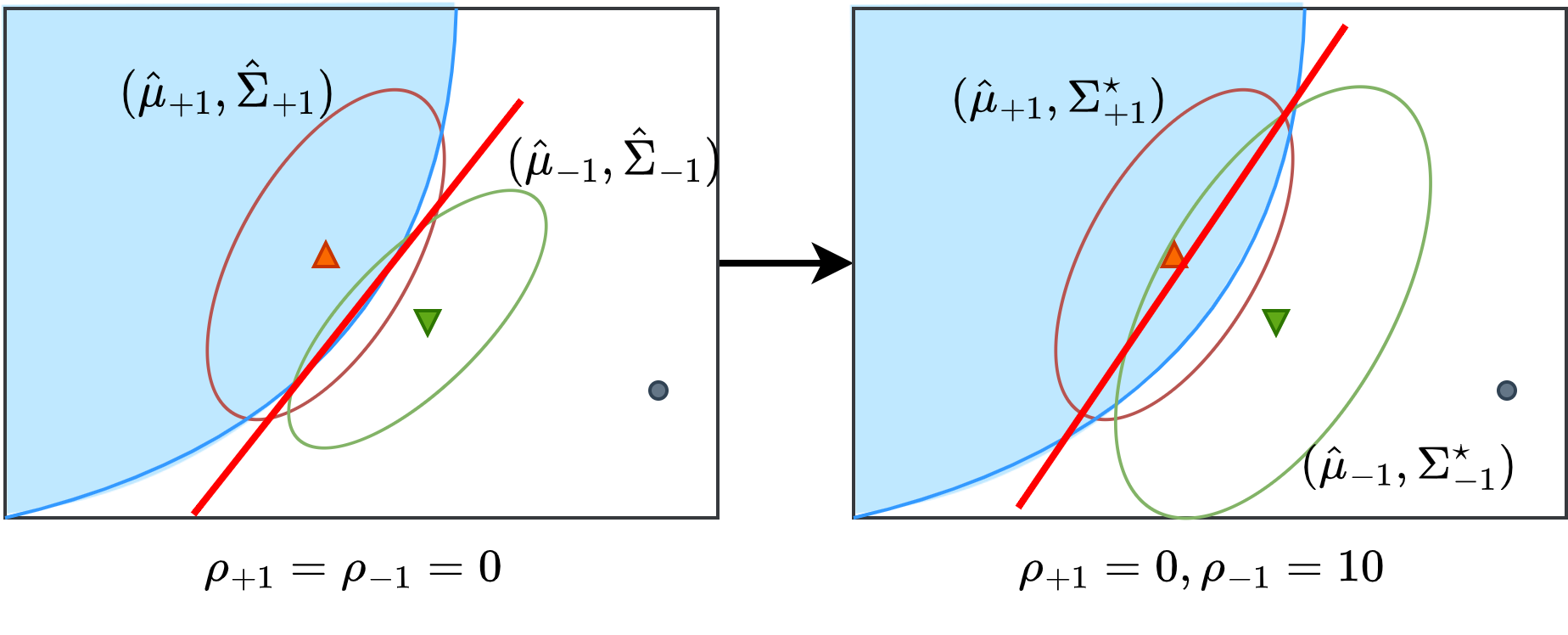
Figure 3. An intuitive explanation of the robustification mechanism. Left: CVAS, right: covariance-robust CVAS with $\rho_{-1}>\rho_{+1}$. By increasing the radius $\rho_{-1}$, the worst-case covariance matrix of the class $-1$ is inflated (bigger green ellipsoid) and shifts the surrogate boundary towards the class $+1$. The projection of the input $x_{0}$ onto the hyperplane will tend to lie deeper into the favorable region and may become more robust to model shifts.

One of the novelties of our framework is the possibility of shifting the linear coverage-validity-aware surrogate towards the region of the favorable class, which induces robust recourse with respect to model shifts in a geometrically intuitive manner (see Figure 3 for an illustration). There is a clear distinction between our framework and the existing method of ROAR [61] and DiRRAc [40]: ROAR and DiRRAc uses a non-robust surrogate in Step (ii) and then formulates a min-max optimization problem in Step (iii) for recourse search. On the contrary, our framework uses a robust surrogate in Step (ii) and then employs a simple recourse search in Step (iii). Using our framework, we can leverage mixed-integer formulations in Step (iii) (e.g., AR [62]) to generate more realistic or actionable, robust recourses. On the contrary, it is unclear how mixed-integer constraints can be integrated into the ROAR or DiRRAc’s min-max formulation.

1.2. Contributions

Motivated by the need to generate robust recourses under various practical considerations such as fairness, explainability, ethics or causality, we propose a novel coverage-validity-aware linear surrogate of the nonlinear boundary of the black-box classifier. Based on ideas from distributionally robust optimization, we develop a variant of the covariance-robust coverage-validity-aware surrogate that can promote robustness against model shifts in the recourse generation task. Unlike some common recourse generation schemes in the literature, our scheme does not require solving min-max problems, and it allows the incorporation of mixed-integer constraints for modelling various practical considerations. Our main contributions can be summarized as follows:

• Coverage-validity-aware surrogate (CVAS). We propose this new linear surrogate approximating the classifier’s decision boundary by balancing the coverage and validity quantities. We establish a strong connection between CVAS and the minimax probability machines proposed by [31] (Proposition 2.1). This connection enables us to identify the surrogate efficiently using second-order cone optimization (Lemma 2.2).

• Covariance-robust CVAS variants: To hedge against potential model shifts, we propose and analyze several robust variants of the CVAS obtained by perturbing the second-order moment information of the synthetic samples around the local decision boundary. We show that the covariance-robust CVAS admits a general form of reformulation (Proposition 3.1). Further, the covariance-robust can be motivated in the parametric Gaussian subspace thanks to the equivalence of the solution between the nonparametric and the parametric Gaussian formulations (Proposition 3.2).

• Covariance-robustness induces regularization. Interestingly, we show that the covariance-robust variants are equivalent to undiscovered regularizations of the MPM. Specifically, using the Bures distance to prescribe the ambiguity set will recover the $\ell_{2}$-regularization scheme (Theorem 4.4). If the ambiguity set is dictated by the Fisher-Rao or LogDet distance, we recover the class reweighting schemes (Theorem 4.7 and 4.10).

• Robust recourse generation: We show that our covariance-robust CVAS can be integrated into the robust recourse generation process. Among multiple variants of the surrogate in this paper, we show that the Fisher-Rao or LogDet surrogates exhibit a more intuitive and interpretable boundary shift in a certain asymptotic sense (Proposition 5.2). This shift aligns better with the coverage-validity trade-off we desire to observe for the recourse generation task; thus, the Fisher-Rao or LogDet CVAS are reasonable surrogates for the recourse generation task. Formulations of the recourse generation problem using CVAS are provided in Section 6.

This paper unfolds as follows. Section 2 and 3 dive deeper into the construction of the CVAS and its robustification to hedge against model shifts. Section 4 presents and compares several variants of covariance-robust surrogates using the Bures, Fisher-Rao, and LogDet distance on the space of covariance matrices. Section 5 studies the asymptotic surrogate as one of the radii grows to infinity, along with the implications on the robust recourse generation task. In Section 6, we demonstrate empirically that our proposed surrogates provide a competitive approximation of the local decision boundary and improve the robustness of the recourse subject to model shifts. All proofs are relegated to the appendix.

2. Coverage-Validity-Aware Linear Surrogate

We present the intuition supporting our construction of the coverage-validity-aware surrogate (CVAS). Given the moment information $(\widehat{\mu}_{y},\widehat{\Sigma}_{y})$ for each $y\in\mathcal{Y}$ that is obtained by the local sampler, we aim to construct a linear surrogate that approximates the local decision boundary of the underlying model and enables the robust generation of recourses in the latter phase. A linear surrogate is parametrized by $\theta=(w,b)\in\mathbb{R}^{d+1}$, $w\neq 0$ with a decision rule

$$\mathcal{C}_{\theta}(x)=\operatorname{sign}(w^{\top}x-b),$$

where $w$ is the slope and $b$ is the intercept.

Figure 4 depicts three potential cases where the relative position of the surrogate to the data clusters differ. The red line depicts the set $\mathbb{H}_{\theta}=\{x\in\mathbb{R}^{d}:w^{\top}x-b=0\}$, termed the decision boundary surrogate: it contains all inputs that lie on the surrogate hyperplane $w^{\top}x=b$. The arrow associated with the line shows the direction toward the positively-predicted hyperplane. The halfspace $\mathbb{H}_{\theta,+1}=\{x\in\mathbb{R}^{d}:\mathcal{C}_{\theta}(x)=+1\}$ on the same side with the arrow contains all inputs which will be predicted positively by the surrogate. Similarly, $\mathbb{H}_{\theta,-1}=\{x\in\mathbb{R}^{d}:\mathcal{C}_{\theta}(x)=-1\}$ is the negatively-predicted halfspace for the surrogate. If we use $\theta$ as a surrogate, any point $x\in\mathbb{H}_{\theta,+1}$ will be considered a feasible recourse under the surrogate’s prediction.

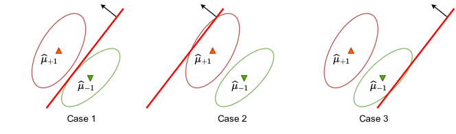
Figure 4. Three scenarios in which the relative position of the surrogate to the data clusters differs. The black arrow indicates the normal vector of the hyperplane.

Next, we define and quantify two qualities of the surrogate associated with the recourse generation.

Coverage. The coverage of a surrogate refers to the surrogate’s ability to capture the valid recourses of the black-box classifier. This coverage can be quantified by the degree of overlap between the set $\mathbb{H}_{\theta,+1}$ (representing possible recourses) and the positive data cluster. We use the Mahalanobis distance from the mean vector of the positive data $\widehat{\mu}_{+1}$ to the decision boundary $\mathbb{H}_{\theta}$ as the proxy to measure this overlap. Specifically, the coverage can be computed as

(2.1) $$\widehat{\mathrm{Co}}_{\widehat{\Sigma}_{+1}}(\theta)\triangleq\inf_{x\in\mathbb{H}_{\theta,-1}}~{}\sqrt{(\widehat{\mu}_{+1}-x)^{\top}\widehat{\Sigma}_{+1}^{-1}(\widehat{\mu}_{+1}-x)},$$

where the Mahalanobis distance is weighted using the data-driven covariance matrix $\widehat{\Sigma}_{+1}$. It is worth noting that we utilize the set $\mathbb{H}_{\theta,-1}$ instead of $\mathbb{H}_{\theta}$ to penalize the case where the surrogate incorrectly predicts the positive center $\widehat{\mu}_{+1}$ (case 2 in Figure 4). In cases 1 and 3, the Mahalanobis distance from the mean of the positive data cluster to the decision boundary $\mathbb{H}_{\theta}$ coincides with that to the set $\mathbb{H}_{\theta,-1}$ (see Lemma B.1 for proof).

Validity. Validity refers to the effectiveness of recourses generated using the surrogate. We measure the validity by assessing the proximity between the set $\mathbb{H}_{\theta,+1}$ and the negative data cluster. Specifically, we employ the following proxy

(2.2) $$\widehat{\mathrm{Va}}_{\widehat{\Sigma}_{-1}}(\theta)\triangleq\inf_{x\in\mathbb{H}_{\theta,+1}}~{}\sqrt{(\widehat{\mu}_{-1}-x)^{\top}\widehat{\Sigma}_{-1}^{-1}(\widehat{\mu}_{-1}-x)},$$

where $\widehat{\Sigma}_{-1}$ is the estimated covariance matrix of the negative samples. A small value of $\widehat{\mathrm{Va}}_{\widehat{\Sigma}_{-1}}(\theta)$ indicates that the recourse set is closer to the cluster of negative samples, implying that the recourses generated using the surrogate are susceptible to perturbations in the ML model’s boundary.

We can relate the relationship between coverage and validity to that of recall and precision, widely used metrics in the ML community. Coverage, similar to recall, measures the quantity or extent of relevant recourses captured by the surrogate model. Validity, similar to precision, measures the quality or reliability of recourses constructed for the surrogate. High coverage suggests that the positively predicted halfspace of a surrogate can encompass a significant portion of the relevant recourses of the underlying model. Meanwhile, high validity indicates that recourses constructed for a surrogate are more likely to remain valid under the underlying model. We can also relate the extreme behavior of the coverage-validity trade-off to the cases of Figure 4. The surrogate plotted in case 2 has $\widehat{\mathrm{Co}}_{\widehat{\Sigma}_{+1}}(\theta)=0$ because $\widehat{\mu}_{+1}\in\mathbb{H}_{\theta,-1}$. Similarly, the surrogate in case 3 has $\widehat{\mathrm{Va}}_{\widehat{\Sigma}_{-1}}(\theta)=0$ because $\widehat{\mu}_{-1}\in\mathbb{H}_{\theta,+1}$. Coverage and validity are thus conflicting criteria and a surrogate with nontrivial coverage-validity trade-off should separate the mean vectors, as in case 1 of Figure 4. Under the assumption that $\widehat{\mu}_{-1}\neq\widehat{\mu}_{+1}$, the separating hyperplane theorem asserts that a linear hyperplane that can separate the mean vectors exists. Hence, we propose a maximin problem to find an appropriate linear surrogate:

(2.3) $$\max\limits_{\theta\in\Theta}~{}\min\left\{\widehat{\mathrm{Co}}_{\widehat{\Sigma}_{+1}}(\theta),~{}\widehat{\mathrm{Va}}_{\widehat{\Sigma}_{-1}}(\theta)\right\}.$$

where $\Theta$ is a set of plausible surrogates defined by

(2.4) $$\Theta\triangleq\{\theta=(w,b)\in\mathbb{R}^{d+1}:w\neq 0\},$$

in which the constraint $w\neq 0$ eliminates trivial surrogates. Note that the minimum problem aims to balance the coverage and validity of the surrogate. This design is reasonable since both measurements are intended to be of similar magnitude.

2.1. Relationship with Minimax Probability Machines

Minimax Probability Machines (MPM) is a binary classification framework pioneered by [31] and extended to Quadratic MPM in [30]. For each class $y\in\mathcal{Y}$, MPM does not assume the specific parametric form of the (conditional) distribution $\widehat{\mathbb{P}}_{y}$ of $X|f(X)=y$. Instead, MPM assumes that we can identify $\widehat{\mathbb{P}}_{y}$ only up to the first two moments, i.e., $\widehat{\mathbb{P}}_{y}$ has mean vector $\widehat{\mu}_{y}\in\mathbb{R}^{d}$ and covariance matrix $\widehat{\Sigma}_{y}\in\mathbb{S}_{+}^{d}$, denoted $\widehat{\mathbb{P}}_{y}\sim(\widehat{\mu}_{y},\widehat{\Sigma}_{y})$. These moments can be estimated from the samples synthesized from the boundary sampler. MPM aims to find a (non-trivial) linear classifier that minimizes the maximum misclassification rate among classes. MPM solves the min-max optimization problem

(2.5) $$\min\limits_{\theta\in\Theta}~{}\max\limits_{y\in\mathcal{Y}}~{}\max\limits_{\widehat{\mathbb{P}}_{y}\sim(\widehat{\mu}_{y},\widehat{\Sigma}_{y})}\widehat{\mathbb{P}}_{y}(\mathcal{C}_{\theta}(X)\neq y),$$

where the set $\Theta$ is defined as in (2.4).

Proposition 2.1 (Equivalence characterization).

The CVAS obtained by solving (2.3) coincides with the MPM obtained by solving (2.5).

Proposition 2.1 establishes an intriguing link between CVAS and MPM. It shows that our surrogate also minimizes the misclassification rate, similar to MPM, by maximizing the coverage and validity quantities. Maximizing the coverage corresponds to minimizing the misclassification rate within the positive class. Meanwhile, the maximization of validity is equivalent to minimizing the misclassification probability within the negative class.

2.2. Solution Procedure

The main instrument to find the coverage-validity-aware surrogate is the result from [31, §2], which provides the optimal solution for the MPM problem. Then, we can leverage the equivalence result from Proposition 2.1 to find the surrogate. Define the set of feasible slopes $\mathcal{W}=\{w\in\mathbb{R}^{d}\backslash\{0\}:\sum_{y\in\mathcal{Y}}yw^{\top}\widehat{\mu}_{y}=1\}$, which is a hyperplane in $\mathbb{R}^{d}$. The next lemma asserts an efficient procedure to compute the surrogate.

Lemma 2.2 (Optimal solution, adapted from [31, §2]).

Let $\widehat{w}$ be an optimal solution to the second-order cone program

(2.6) $$\min\limits_{w\in\mathcal{W}}~{}\sum\nolimits_{y\in\mathcal{Y}}\sqrt{w^{\top}\widehat{\Sigma}_{y}w},$$

and let $\widehat{\kappa}=\big{(}\sum\nolimits_{y\in\mathcal{Y}}\sqrt{\widehat{w}^{\top}\widehat{\Sigma}_{y}\widehat{w}}\big{)}^{-1}$, and $\widehat{b}=\widehat{w}^{\top}\widehat{\mu}_{+1}-\widehat{\kappa}\sqrt{\widehat{w}^{\top}\widehat{\Sigma}_{+1}\widehat{w}}$. Then $\widehat{\theta}=(\widehat{w},\widehat{b})$ solves the coverage-validity-aware surrogate problem (2.3).

In this paper, we refer to the second-order cone program (2.6) as the nominal problem.

3. Coverage-Validity-Aware Linear Surrogate under Model Shifts

The CVAS presented in the previous section is adapted to the black-box ML model $f$. Each synthetic sample is associated with a pseudo-label generated from $f$, which helps define the data clusters for each class and guides the surrogate problem (2.3). A typical recourse generation framework often assumes that the model $f$ does not change over time. Nevertheless, this assumption is usually violated in practice. To model the potential shifts of the model $f$, one can opt for modeling the decision boundary of $f$ and how this boundary may alter temporally. Unfortunately, representing a nonlinear decision boundary and its possible shifts poses a significant technical challenge. Further, because our framework aims to find an approximate linear surrogate $\mathcal{C}_{\theta}$ represented by a $(d+1)$ dimensional parameter, tracing the nonlinear shifts of the decision boundary of $f$ is a likely overload of unnecessary information.

We propose to model the potential shifts of the black-box ML model $f$ using the shifts of the data clusters. Specifically, we are not modeling how each data pseudolabel may shift but how the aggregated second-order moment information of the data may change. To do this, we suppose that the covariance matrix of the $y$-class data cluster may shift to a value $\Sigma_{y}$, which can be different from the nominal value $\widehat{\Sigma}_{y}$. These shifts of $\Sigma_{y}$ away from $\widehat{\Sigma}_{y}$ represent the second-order shift of the future ML model away from the current model $f$. The shift amount is quantified using the function $\varphi$, which measures the dissimilarity between covariance matrices. The function $\varphi$ should be a divergence: it is non-negative and $\varphi(\Sigma_{y}\parallel\widehat{\Sigma}_{y})=0$ if and only if $\Sigma_{y}=\widehat{\Sigma}_{y}$. We also need to specify the shift budgets $\rho_{y}$, which dictate the maximal amount of covariance shifts possible for the $y$-class data cluster.

Motivated by the success of (distributionally) robust optimization in machine learning and ethical AI [60, 67], we introduce the covariance-robust CVAS, which is defined as the solution of the adversarial trade-off balancing problem

(3.1) $$\max\limits_{\theta\in\Theta}~{}\min\limits_{\Sigma_{y}\in\mathbb{S}_{++}^{d}:\varphi(\Sigma_{y}\parallel\widehat{\Sigma}_{y})\leq\rho_{y}~{}\forall y}~{}\min\left\{~{}\widehat{\mathrm{Co}}_{\Sigma_{+1}}(\theta),\widehat{\mathrm{Va}}_{\Sigma_{-1}}(\theta)\right\},$$

where we make explicit the dependence of the coverage and validity measures on the covariance weighting matrices $\Sigma_{+1}$ and $\Sigma_{-1}$, respectively. The covariance-robust CVAS (3.1) alleviates the model shifts problem by injecting an additional layer of conservativeness to the surrogate: the surrogate now maximizes the worst-case values of the coverage and validity measures, subject to all possible perturbations of the covariance matrix of each data cluster. One can view problem (3.1) as a zero-sum game between the surrogate generator and a fictitious adversarial opponent: the surrogate generator aims to find a parameter $\theta$ that can balance the coverage and validity trade-off. In contrast, the opponent can shift the covariance matrices of the data clusters to reduce the coverage and validity of the surrogate.

There are now two main questions about the new family of covariance-robust CVASes: (i) How could we solve problem (3.1) efficiently? (ii) how could we choose the divergence $\varphi$? In Section 3.1, we establish a general result on the solution method of problem (3.1) for a generic choice of $\varphi$. Then, Section 3.2 motivates to choose $\varphi$ using statistical divergence between Gaussian distributions.

3.1. Equivalence and Solution Procedure

Proposition 2.1 establishes an equivalence between the CVAS and the MPM. It is reasonable to predict that the (covariance-robust) CVAS should be equivalent to a certain form of MPM under probability misspecification. We will establish this equivalence in this section. We first define the ambiguity set

$$\mathbb{U}_{y}^{\varphi}(\widehat{\mathbb{P}}_{y})=\{\mathbb{P}_{y}:~{}\mathbb{P}_{y}\sim(\widehat{\mu}_{y},\Sigma_{y}),~{}\varphi(\Sigma_{y}\parallel\widehat{\Sigma}_{y})\leq\rho_{y}\}$$

for each conditional distribution respective to the $y$-label. Each $\mathbb{U}_{y}^{\varphi}(\widehat{\mathbb{P}}_{y})$ is a non-parametric set: it contains all distributions supported on $\mathbb{R}^{d}$ with mean $\widehat{\mu}_{y}$ and covariance matrix $\Sigma_{y}$, whereas the $\Sigma_{y}$ resides in the neighborhood of radius $\rho_{y}$ from the nominal values $\widehat{\Sigma}_{y}$. Consider now the MPM under probability misspecification, which is a distributionally robust optimization problem:

(3.2) $$\min\limits_{\theta\in\Theta}~{}\max\limits_{y\in\mathcal{Y}}~{}\max\limits_{\mathbb{P}_{y}\in\mathbb{U}^{\varphi}_{y}(\widehat{\mathbb{P}}_{y})}\mathbb{P}_{y}(\mathcal{C}_{\theta}(X)\neq y).$$

The goal of problem (3.2) is to find a linear classifier that minimizes the worst-case maximal misclassification rate among classes, where the conditional data generating distributions are confined to the ambiguity sets $\mathbb{U}_{y}^{\varphi}(\widehat{\mathbb{P}}_{y})$. Problem (3.2) is not new: in fact, it was first proposed by [30] but with $\varphi$ being the squared Frobenius distance $\varphi(\Sigma_{y}\parallel\widehat{\Sigma}_{y})=\operatorname{Tr}\big{[}(\Sigma_{y}-\widehat{\Sigma}_{y})^{2}\big{]}$.

Now, we will establish that the optimal solution of problem (3.1) is equivalent to the optimal solution of problem (3.2). This equivalence is established for any arbitrary divergence function $\varphi$. Toward this goal, for any $y\in\mathcal{Y}$, define $\tau_{y}:\mathbb{R}^{d}\to\mathbb{R}$ as

(3.3) $$\tau_{y}^{\varphi}(w)\triangleq\max\limits_{\Sigma_{y}\in\mathbb{S}_{+}^{d}:\varphi(\Sigma_{y}\parallel\widehat{\Sigma}_{y})\leq\rho_{y}}\sqrt{w^{\top}\Sigma_{y}w}.$$

We now provide a generalized equivalence result and a reformulation of the CVAS under model shifts problem (3.1).

Proposition 3.1 (Robust surrogate under model shifts).

Let $\varphi$ be an arbitrary divergence on the space of covariance matrices. The CVAS under model shifts obtained by solving (3.1) coincides with the MPM under probability misspecification obtained by solving (3.2). Moreover, let $w^{\varphi}$ be the optimal solution to the problem

$$\min\limits_{w\in\mathcal{W}}~{}\sum\nolimits_{y\in\mathcal{Y}}\tau_{y}^{\varphi}(w),$$

and let $\kappa^{\varphi}=\big{(}\displaystyle\sum\nolimits_{y\in\mathcal{Y}}\tau_{y}^{\varphi}(w^{\varphi})\big{)}^{-1}$, and $b^{\varphi}=(w^{\varphi})^{\top}\widehat{\mu}_{+1}-\kappa^{\varphi}\tau_{+1}^{\varphi}(w^{\varphi})$. Then $\theta^{\varphi}=(w^{\varphi},b^{\varphi})$ solves the covariance-robust CVAS problem (3.1).

This equivalence result provides a generic solution procedure to find the covariance-robust CVAS, provided that we can evaluate the function $\tau_{y}^{\varphi}$ in (3.3).

3.2. Equivalence under Gaussian Assumptions

When $\varphi$ is chosen as the squared Frobenius distance, we recover the Quadratic MPM first studied in [30]. As we will delineate in Section 4.1, the Quadratic MPM will give rise to a Quadratic surrogate. Nevertheless, the squared Frobenius distance is not statistically meaningful: it does not coincide with any distance between probability distributions with the corresponding covariance information. On the upside, the connection between the MPM framework and our surrogate can be exploited to design many versions of the surrogate by simply choosing different divergences $\varphi$. One thus can consider more principled approaches of choosing $\varphi$ by leveraging the distributional properties of the MPM formulation.

This section shows that the MPM under probability misspecification problem (3.2) is invariant with the Gaussian information. Put differently, the solution to problem (3.2) does not change if a parametric Gaussian assumption is imposed on the conditional distributions. To see this, define a parametric ambiguity set constructed on the space of Gaussian distributions of the form

$$\mathcal{U}_{y}^{\mathcal{N}}(\widehat{\mathbb{P}}_{y})=\left\{\mathbb{P}_{y}\in\mathcal{P}(\mathcal{X}):~{}\mathbb{P}_{y}\sim\mathcal{N}(\widehat{\mu}_{y},\Sigma_{y}),~{}\varphi(\Sigma_{y}\parallel\widehat{\Sigma}_{y})\leq\rho_{y}\right\},$$

wherein any distribution in this set is Gaussian. Consider the Gaussian-robust MPM problem

(3.4) $$\min\limits_{\theta\in\Theta}~{}\max\limits_{y\in\mathcal{Y}}~{}\max\limits_{\mathbb{P}_{y}\in\mathcal{U}_{y}^{\mathcal{N}}(\widehat{\mathbb{P}}_{y})}~{}\mathbb{P}_{y}(\mathcal{C}_{\theta}(X)\neq y).$$

The only difference between problem (3.4) and problem (3.2) is the Gaussian specification of the ambiguity sets. Nevertheless, the next result asserts that the solutions to the two problems coincide.

Proposition 3.2 (Gaussian equivalence).

The optimizer $\theta^{\varphi}=(w^{\varphi},b^{\varphi})$ in Proposition 3.1 also solves the Gaussian-robust MPM problem (3.4).

Proposition 3.2 implies that it suffices to restrict the MPM problem to Gaussian misspecification. It thus justifies using divergences $\varphi$ induced by some dissimilarity measures between Gaussian distributions. This leads to a family of surrogates, as we will explore in the next section.

4. Examples of Robust Surrogates

We discuss in this section several versions of the CVASes under model shifts, including the Quadratic CVAS in Section 4.1, the Bures CVAS in Section 4.2, the Fisher-Rao CVAS in Section 4.3, and the LogDet CVAS in Section 4.4.

4.1. Quadratic Surrogate

First, consider the perturbation of the covariance matrix using the quadratic divergence.

Definition 4.1 (Quadratic divergence).

Given two positive semidefinite matrices $\Sigma$, $\widehat{\Sigma}\in\mathbb{S}_{+}^{d}$, the quadratic divergence between them is $\mathds{Q}(\Sigma\parallel\widehat{\Sigma})=\operatorname{Tr}\big{[}(\Sigma-\widehat{\Sigma})^{2}\big{]}$.

The divergence $\mathds{Q}$ is the squared Frobenius norm of $\Sigma-\widehat{\Sigma}$; thus $\mathds{Q}$ is non-negative and vanishes to zero if and only if $\Sigma=\widehat{\Sigma}$, so it is a divergence on $\mathbb{S}_{+}^{d}$. The Quadratic CVAS has the below form.

Theorem 4.2 (Quadratic surrogate).

Suppose that $\varphi\equiv\mathds{Q}$. Let $w^{\mathds{Q}}$ be a solution to the problem

(4.1) $$\min\limits_{w\in\mathcal{W}}~{}\displaystyle\sum\nolimits_{y\in\mathcal{Y}}\sqrt{w^{\top}(\widehat{\Sigma}_{y}+\sqrt{\rho_{y}}I)w}.$$

Then $\theta^{\mathds{Q}}=(w^{\mathds{Q}},b^{\mathds{Q}})$ solves the surrogate problem under model shifts (3.1), with

$$\kappa^{\mathds{Q}} =\left(\sum\nolimits_{y\in\mathcal{Y}}\sqrt{(w^{\mathds{Q}})^{\top}(\widehat{\Sigma}_{y}+\sqrt{\rho_{y}}I)w^{\mathds{Q}}}\right)^{-1},$$

$$\text{and}\qquad b^{\mathds{Q}} =(w^{\mathds{Q}})^{\top}\widehat{\mu}_{+1}-\kappa^{\mathds{Q}}\sqrt{(w^{\mathds{Q}})^{\top}(\widehat{\Sigma}_{+1}+\sqrt{\rho_{+1}}I)w^{\mathds{Q}}}.$$

Theorem 4.2 is obtained by exploiting the result from [30], which asserts the optimal form of the Quadratic MPM. We present Theorem 4.2 mainly for comparison purposes against our new statistical variants. Problem (4.1) can be considered as a regularization of the nominal problem (2.6): each matrix $\widehat{\Sigma}_{y}$ is added with a diagonal matrix $\sqrt{\rho_{y}}I$, making the matrix better conditioned. This is equivalently known as inverse regularization, which ensures invertibility when $\widehat{\Sigma}_{y}$ is low-rank and $\rho_{y}>0$.

4.2. Bures Surrogate

We now explore a variant of a statistically-motivated surrogate using Bures divergence as $\varphi$.

Definition 4.3 (Bures divergence).

Given two positive semi-definite matrices $\Sigma$, $\widehat{\Sigma}\in\mathbb{S}_{+}^{d}$, the Bures divergence between them is $\mathds{B}(\Sigma\parallel\widehat{\Sigma})=\operatorname{Tr}\big{[}\Sigma+\widehat{\Sigma}-2(\widehat{\Sigma}^{\frac{1}{2}}\Sigma\widehat{\Sigma}^{\frac{1}{2}})^{\frac{1}{2}}\big{]}$.

It can be shown that $\mathds{B}$ is symmetric and non-negative, and it vanishes to zero if and only if $\Sigma=\widehat{\Sigma}$. As such, $\mathds{B}$ is a divergence on the space of positive semidefinite matrices. Additionally, it is equivalent to the squared type-2 Wasserstein distance between two Gaussian distributions with the same mean vector and covariance matrices $\Sigma$ and $\widehat{\Sigma}$ [45, 20, 18]. Next, we state the form of the Bures surrogate.

Theorem 4.4 (Bures surrogate).

Suppose that $\varphi\equiv\mathds{B}$. Let $w^{\mathds{B}}$ be the solution to the problem

(4.2) $$\min\limits_{w\in\mathcal{W}}~{}\displaystyle\sum\nolimits_{y\in\mathcal{Y}}\sqrt{w^{\top}\widehat{\Sigma}_{y}w}+\big{(}\sum\nolimits_{y\in\mathcal{Y}}\rho_{y}\big{)}\|w\|_{2}.$$

Then $\theta^{\mathds{B}}=(w^{\mathds{B}},b^{\mathds{B}})$ solves the surrogate problem under model shifts (3.1), where

$$\kappa^{\mathds{B}} =\left(\sum\nolimits_{y\in\mathcal{Y}}\sqrt{(w^{\mathds{B}})^{\top}\widehat{\Sigma}_{y}w^{\mathds{B}}}+\big{(}\sum\nolimits_{y\in\mathcal{Y}}\rho_{y}\big{)}\|w^{\mathds{B}}\|_{2}\right)^{-1},$$

$$\text{and}\qquad b^{\mathds{B}} =(w^{\mathds{B}})^{\top}\widehat{\mu}_{+1}-\kappa^{\mathds{B}}(\sqrt{(w^{\mathds{B}})^{\top}\widehat{\Sigma}_{+1}w^{\mathds{B}}}+\rho_{+1}\|w^{\mathds{B}}\|_{2}).$$

Theorem 4.4 unveils a fundamental connection between robustness and regularization: if we perturb the covariance matrices using the Bures divergence, the resulting optimization problem (4.2) is an $l_{2}$-regularization of the problem (2.6). This connection aligns with previous observations showing the equivalence between regularization schemes and optimal transport robustness [55, 9, 29]. To prove Theorem 4.4, we provide in Proposition 4.5 a result that asserts the analytical form of $\tau_{y}^{\mathds{B}}(w)$. The proof of Theorem 4.4 follows by combining Propositions 3.1 and 4.5.

Proposition 4.5 (Bures divergence).

If $\varphi\equiv\mathds{B}$, then $\tau_{y}^{\mathds{B}}(w)=\rho_{y}\|w\|_{2}+\sqrt{w^{\top}\widehat{\Sigma}_{y}w}$ for all $y\in\mathcal{Y}$.

4.3. Fisher-Rao Surrogate

The second new variant of a statistically-motivated surrogate is obtained by taking $\varphi$ as the Fisher-Rao divergence.

Definition 4.6 (Fisher-Rao distance).

Given two positive definite matrices $\Sigma$, $\widehat{\Sigma}\in\mathbb{S}_{++}^{d}$, the Fisher-Rao distance between them is $\mathds{F}(\Sigma,\widehat{\Sigma})=\|\log(\widehat{\Sigma}^{-\frac{1}{2}}\Sigma\widehat{\Sigma}^{-\frac{1}{2}})\|_{2}$, where $\log(\cdot)$ is the matrix logarithm.

The Fisher-Rao distance enjoys many desirable properties. In particular, it is invariant to inversion and congruence, i.e., for any $\Sigma,~{}\widehat{\Sigma}\in\mathbb{S}_{++}^{d}$ and invertible $A\in\mathbb{R}^{d\times d}$, $\mathds{F}(\Sigma,\widehat{\Sigma})=\mathds{F}(\Sigma^{-1},\widehat{\Sigma}^{-1})=\mathds{F}(A\Sigma A^{\top},A\widehat{\Sigma}A^{\top})$. Such invariances are statistically meaningful because it implies that the results remain unchanged if we reparametrize the problem with an inverse covariance matrix (instead of the covariance matrix), or if we apply a change of basis to the data space $\mathcal{X}$. It is shown that $\mathds{F}$ is the unique Riemannian distance (up to scaling) on the cone $\mathbb{S}_{++}^{d}$ with such invariances [53]. Next, we assert the form of the Fisher-Rao surrogate.

Theorem 4.7 (Fisher-Rao surrogate).

Suppose that $\varphi\equiv\mathds{F}$. Let $w^{\mathds{F}}$ be the solution of the following problem

(4.3) $$\min\limits_{w\in\mathcal{W}}~{}\sum\nolimits_{y\in\mathcal{Y}}\exp\left(\frac{\rho_{y}}{2}\right)\sqrt{w^{\top}\widehat{\Sigma}_{y}w}.$$

Then $\theta^{\mathds{F}}=(w^{\mathds{F}},b^{\mathds{F}})$ solves the surrogate problem under model shifts (3.1), where

$$\kappa^{\mathds{F}} \!=\!\big{(}\sum_{y\in\mathcal{Y}}\exp\left(\frac{\rho_{y}}{2}\right)\sqrt{(w^{\mathds{F}})^{\top}\widehat{\Sigma}_{y}w^{\mathds{F}}}\big{)}^{-1}$$

$$\text{and}\quad b^{\mathds{F}} \!=\!(w^{\mathds{F}})^{\top}\widehat{\mu}_{+1}-\kappa^{\mathds{F}}\exp\left(\frac{\rho_{+1}}{2}\right)\sqrt{(w^{\mathds{F}})^{\top}\widehat{\Sigma}_{+1}w^{\mathds{F}}}.$$

Theorem 4.7 divulges another foundational connection between robustness and regularization: if we construct the ambiguity sets for the covariance matrices using the Fisher-Rao distance, the resulting optimization problem (4.3) is a reweighted version of the nominal problem (2.6). Each term $(w^{\top}\widehat{\Sigma}_{y}w)^{\frac{1}{2}}$ is assigned a weight $\exp(\rho_{y}/2)$, which is proportional to the radius $\rho_{y}$. This connection aligns with previous observations highlighting the equivalence between reweighting schemes and distributional robustness [4, 3, 39, 24]. To prove Theorem 4.7, we derive an analytical expression of $\tau_{y}^{\mathds{F}}(w)$ in Proposition 4.8. The proof of Theorem 4.7 follows by combining Proposition 3.1 and Proposition 4.8.

Proposition 4.8 (Fisher-Rao distance).

If $\varphi\equiv\mathds{F}$, then $\tau_{y}^{\mathds{F}}(w)=\exp\left(\frac{\rho_{y}}{2}\right)(w^{\top}\widehat{\Sigma}w)^{\frac{1}{2}}$ for all $y\in\mathcal{Y}$.

4.4. LogDet Surrogate

Last, we consider the case when $\varphi$ is the Log-Determinant (LogDet) divergence, which is a distance-like measure closely related to information theory, see [44, 70].

Definition 4.9 (LogDet divergence).

Given two positive definite matrices $\Sigma$, $\widehat{\Sigma}\in\mathbb{S}_{++}^{d}$, the log-determinant divergence between them is $\mathds{D}(\Sigma\parallel\widehat{\Sigma})=\operatorname{Tr}\big{[}\Sigma\widehat{\Sigma}^{-1}\big{]}-\log\det(\Sigma\widehat{\Sigma}^{-1})-d$.

It can be shown that $\mathds{D}$ is a divergence because it is non-negative and vanishes to zero if and only if $\Sigma=\widehat{\Sigma}$. However, $\mathds{D}$ is not symmetric, and in general, we have $\mathds{D}(\Sigma\parallel\widehat{\Sigma})\neq\mathds{D}(\widehat{\Sigma}\parallel\Sigma)$. The LogDet divergence $\mathds{D}$ is related to the relative entropy: it is equal to the Kullback-Leibler divergence between two Gaussian distributions with the same mean vector and covariance matrices $\Sigma$ and $\widehat{\Sigma}$. We now provide the form of the LogDet surrogate problem.

Theorem 4.10 (LogDet surrogate).

Suppose that $\varphi\equiv\mathds{D}$. Let $w^{\mathds{D}}$ be the optimal solution of the following second-order cone problem

(4.4) $$\min\limits_{w\in\mathcal{W}}~{}\sum_{y\in\mathcal{Y}}\sqrt{c_{y}}\sqrt{w^{\top}\widehat{\Sigma}_{y}w},$$

where $c_{y}=-W_{-1}(-\exp(-\rho_{y}-1))$ and $W_{-1}$ is the Lambert-W function for the branch $-1$. Then $\theta^{\mathds{D}}=(w^{\mathds{D}},b^{\mathds{D}})$ solves the surrogate problem under model shifts (3.1), where

$$\kappa^{\mathds{D}} =\displaystyle\frac{1}{\sum_{y\in\mathcal{Y}}\sqrt{c_{y}}\sqrt{(w^{\mathds{D}})^{\top}\widehat{\Sigma}_{y}w^{\mathds{D}}}}$$

$$\text{and}\quad b^{\mathds{D}} =(w^{\mathds{D}})^{\top}\widehat{\mu}_{+1}-\kappa^{\mathds{D}}\sqrt{c_{+1}}\sqrt{(w^{\mathds{D}})^{\top}\widehat{\Sigma}_{+1}w^{\mathds{D}}}.$$

Theorem 4.10 shows that the LogDet divergence induces a similar reweighting scheme as the Fisher-Rao MPM. The proof of Theorem 4.10 follows by combining Proposition 4.11 below, which provides the analytical form of $\tau_{y}^{\mathds{D}}(w)$, with Proposition 3.1.

Proposition 4.11 (LogDet divergence).

Suppose that $\varphi\equiv\mathds{D}$, then for any $y\in\mathcal{Y}$, we have

$$\tau_{y}^{\mathds{D}}(w)=\sqrt{-W_{-1}(-\exp(-\rho_{y}-1))}\sqrt{w^{\top}\widehat{\Sigma}_{y}w},$$

where $W_{-1}$ is the Lambert-W function for the branch $-1$.

5. Asymptotic Surrogates

The preceding section shows that employing various divergences to prescribe the ambiguity sets leads to different regularizations of the vanilla CVAS. This section studies the asymptotic surrogates to examine how these surrogates behave as the perturbation radii grow. These analyses provide valuable insights into the impact of the covariance-robust surrogates on the subsequent recourse generation phase and offer guidance for selecting the surrogate that best suits the task of robust recourse generation.

Proposition 5.1 (Asymptotic surrogates).

Fix $y\in\mathcal{Y}$, let $-y$ be its opposite class, and let $a\triangleq\sum_{y^{\prime}\in\mathcal{Y}}y^{\prime}\widehat{\mu}_{y^{\prime}}$. Suppose that $\rho_{-y}$ remains constant, then as $\rho_{y}\to\infty$, the optimal solution $\theta^{\varphi}_{\rho_{y}}=(w_{\rho_{y}}^{\varphi},b_{\rho_{y}}^{\varphi})$ of problem (3.1), parametrized by $\rho_{y}$, can be expressed as follows.

1. If $\varphi$ is the Quadratic or Bures distance, then

   $$w_{\rho_{y}}^{\varphi}\to w_{\infty,y}^{\varphi}\triangleq\frac{a}{\|a\|_{2}^{2}}\quad\text{and}\quad b_{\rho_{y}}^{\varphi}\to b_{\infty,y}^{\varphi}\triangleq(w_{\infty,y}^{\varphi})^{\top}\widehat{\mu}_{y}-y.$$

2. If $\varphi$ is the Fisher-Rao or LogDet distance, then

   $$w_{\rho_{y}}^{\varphi}\to w_{\infty,y}^{\varphi}\triangleq\frac{\widehat{\Sigma}_{y}^{-1}a}{a^{\top}\widehat{\Sigma}_{y}^{-1}a}\quad\text{and}\quad b_{\rho_{y}}^{\varphi}\to b_{\infty,y}^{\varphi}\triangleq(w_{\infty,y}^{\varphi})^{\top}\widehat{\mu}_{y}-y.$$

Because the intercept $b_{\rho_{y}}^{\varphi}$ tends towards $b_{\infty,y}^{\varphi}=(w_{\infty,y}^{\varphi})^{\top}\widehat{\mu}_{y}-y$, the asymptotic hyperplane defined by ($w_{\infty,y}^{\varphi},b_{\infty,y}^{\varphi})$ is then characterized by the linear equation $(w_{\infty,y}^{\varphi})^{\top}(x-\widehat{\mu}_{y})+y=0$. This equation identifies a hyperplane passing through $\widehat{\mu}_{-y}$ as $\sum_{y\in\mathcal{Y}}yw^{\top}\widehat{\mu}_{y}=1$.

Proposition 5.1(i) shows that the Quadratic surrogate and the Bures surrogate are asymptotically equivalent even though they induce different regularizations of the vanilla surrogate (2.6). Moreover, for these two divergences, the asymptotic slope depends only on the aggregated quantity $\sum\nolimits_{y^{\prime}\in\mathcal{Y}}y^{\prime}\widehat{\mu}_{y^{\prime}}$, but not on the specification of $y$. On the contrary, the asymptotic hyperplane of the Fisher-Rao and LogDet surrogate depends explicitly on the covariance matrix $\widehat{\Sigma}_{y}$. The following result asserts the explicit trade-off between coverage and validity when calibrating the Fisher-Rao radii.

Proposition 5.2 (Coverage-validity trade-off).

Let $\rho=(\rho_{+1},\rho_{-1})$ and $\rho^{\prime}=(\rho^{\prime}_{+1},\rho^{\prime}_{-1})$ be two sets of radii such that $\rho_{+1}=\rho_{+1}^{\prime}=0$ and $\rho_{-1}>\rho_{-1}^{\prime}\geq 0$. Let $\theta_{\rho}=(w_{\rho},b_{\rho})$ and $\theta_{\rho^{\prime}}=(w_{\rho^{\prime}},b_{\rho^{\prime}})$ be the two optimal hyperplanes obtained by solving the Fisher-Rao surrogate problem (4.3) with radii $\rho$ and $\rho^{\prime}$, respectively. Then

$$\widehat{\mathrm{Co}}_{\widehat{\Sigma}_{+1}}(\theta_{\rho})<\widehat{\mathrm{Co}}_{\widehat{\Sigma}_{+1}}(\theta_{\rho^{\prime}})\quad\text{and}\quad\widehat{\mathrm{Va}}_{\widehat{\Sigma}_{-1}}(\theta_{\rho})>\widehat{\mathrm{Va}}_{\widehat{\Sigma}_{-1}}(\theta_{\rho^{\prime}}).$$

Note that a similar result to Proposition 5.2 also holds for the robust LogDet surrogate because the LogDet surrogate also recovers the class-reweighting regularization. Proposition 5.2 suggests that, by fixing $\rho_{+1}=0$ and increasing $\rho_{-1}$, our linear surrogate exhibits higher validity but lower coverage. The increased validity indicates that the generated recourse is more likely to be valid when applied to the underlying model. However, the reduced coverage suggests a potential increase in the cost of implementing recourses due to the decreased overlap between the recourse sets of the surrogate and the underlying model. We will probe this rise in cost in the experimental section.

It is worth noting further that the validity inequality does not hold universally for Quadratic and Bures divergences. To illustrate this, we consider the following counterexample.

Counterexample 5.3.

Consider the following nominal mean vector and covariance matrix for each class:

$$\widehat{\mu}_{-1}=\begin{pmatrix}0\\ 0\end{pmatrix},~{}\widehat{\Sigma}_{-1}=\begin{bmatrix}5&2\\ 2&1\end{bmatrix}\quad\text{and}\quad\widehat{\mu}_{+1}=\begin{pmatrix}10\\ 0\\ \end{pmatrix},~{}\widehat{\Sigma}_{+1}=\begin{bmatrix}5&2\\ 2&1\end{bmatrix}.$$

The nominal surrogate obtained by Lemma 2.2 with $\rho_{+1}^{\prime}=\rho_{-1}^{\prime}=0$ is given by $x_{1}-2x_{2}-5=0$, which achieves $\widehat{\mathrm{Va}}_{\widehat{\Sigma}_{-1}}(\theta_{\rho^{\prime}})=5$. Fixing $\rho_{+1}=0$ and letting $\rho_{-1}\to\infty$, Propositions 5.1 asserts that both Quadratic and Bures surrogates converge to the hyperplane prescribed by $x_{1}-10=0$, which attains $\widehat{\mathrm{Va}}_{\widehat{\Sigma}_{-1}}(\theta_{\rho})=\frac{10}{\sqrt{5}}$. Therefore, $\widehat{\mathrm{Va}}_{\widehat{\Sigma}_{-1}}(\theta_{\rho})<\widehat{\mathrm{Va}}_{\widehat{\Sigma}_{-1}}(\theta_{\rho^{\prime}})$ even though $\rho_{-1}>\rho_{-1}^{\prime}$, meaning that the Quadratic and Bures surrogates violate the validity inequality.

Meanwhile, if we use the Fisher-Rao surrogate, the optimal surrogate when $\rho_{-1}\to\infty$ is characterized by the hyperplane $x_{1}-2x_{2}-10=0$. This surrogate achieves $\widehat{\mathrm{Va}}_{\widehat{\Sigma}_{-1}}(\theta_{\rho})=10$, which is consistent with Proposition 5.2. Figure 5 illustrates and compares the asymptotic hyperplanes of three surrogates.

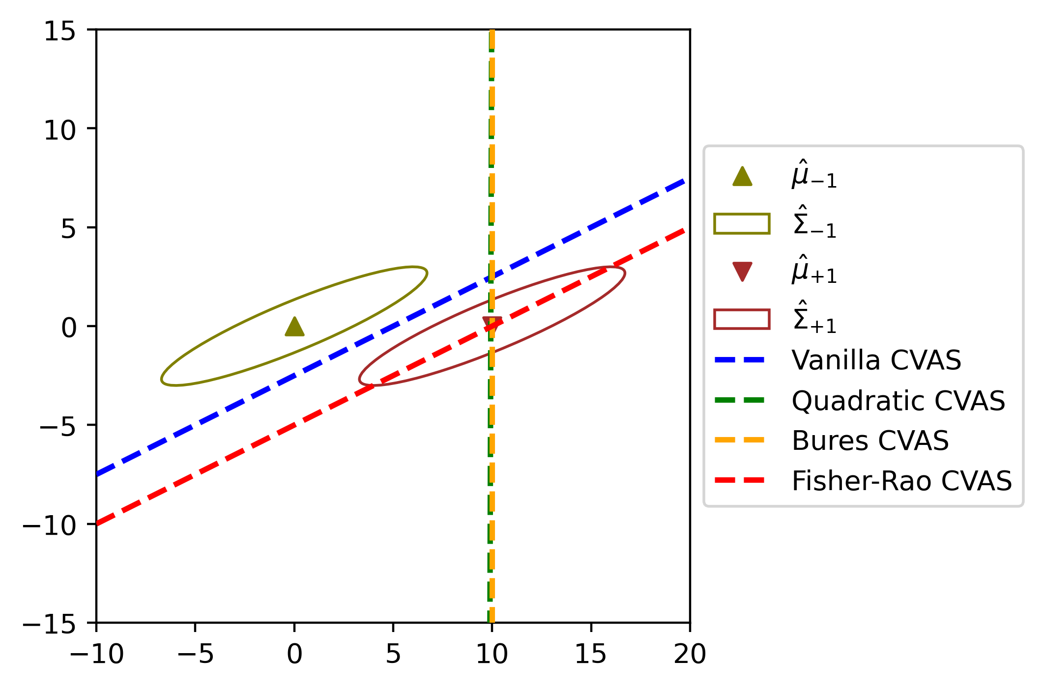
Figure 5. Comparison of the asymptotic hyperplanes of Quadratic, Bures, and Fisher-Rao surrogates as $\rho_{-1}\to\infty$.

6. Numerical Experiments

The goals of the experiments are two-fold: First, we investigate the sensitivity and fidelity of our CVASes compared with LIME [50], a widely-used surrogate in recourse literature. Second, we empirically demonstrate that CVAS can be integrated into the recourse generation problem to promote robustness. More extensive experiments, including comparisons with RBR [41] and DiRRAc [40], are provided in Appendix A.2.

We provide the information regarding the architecture we use for the black-box model, as well as the dataset and the data processing.

Classifier. To construct the black-box classifier, we use a three-layer MLP with 20, 50, 20 nodes and ReLU activation in each consecutive layer. We use a sigmoid function in the last layer to produce probabilities. We use the binary cross-entropy to train this classifier, solved using the Adam optimizer and 1000 epochs.

Dataset. We evaluate our framework using popular real-world datasets for algorithmic recourse: German Credit [16, 21], Small Bussiness Administration (SBA) [34], and Student performance [13]. Each dataset contains two sets of data (the present data $D_{1}$ and the shifted data $D_{2}$). The shifted dataset $D_{2}$ could capture the correction shift (for the German dataset), temporal shift (SBA), or geospatial shift (Student). For each dataset, we use $80\%$ of the instances in the present data $D_{1}$ to train an underlying classifier, and the remaining instances are used as input to generate recourses. The shifted data $D_{2}$ is used to train future classifiers to evaluate the validity of the recourse; see further details in Section 6.2.

Naming convention. The Quadratic surrogate obtained in Theorem 4.2 is denoted QUAD-CVAS, the Bures surrogate obtained in Theorem 4.4 is denoted BW-CVAS, and the Fisher-Rao surrogate obtained in Theorem 4.7 is denoted FR-CVAS.

6.1. Sensitivity and Fidelity of CVAS

In the first set of experiments, we evaluate and compare covariance-robust CVASes against LIME [50] in terms of their sensitivity with respect to the input and their fidelity with respect to the current classifier.

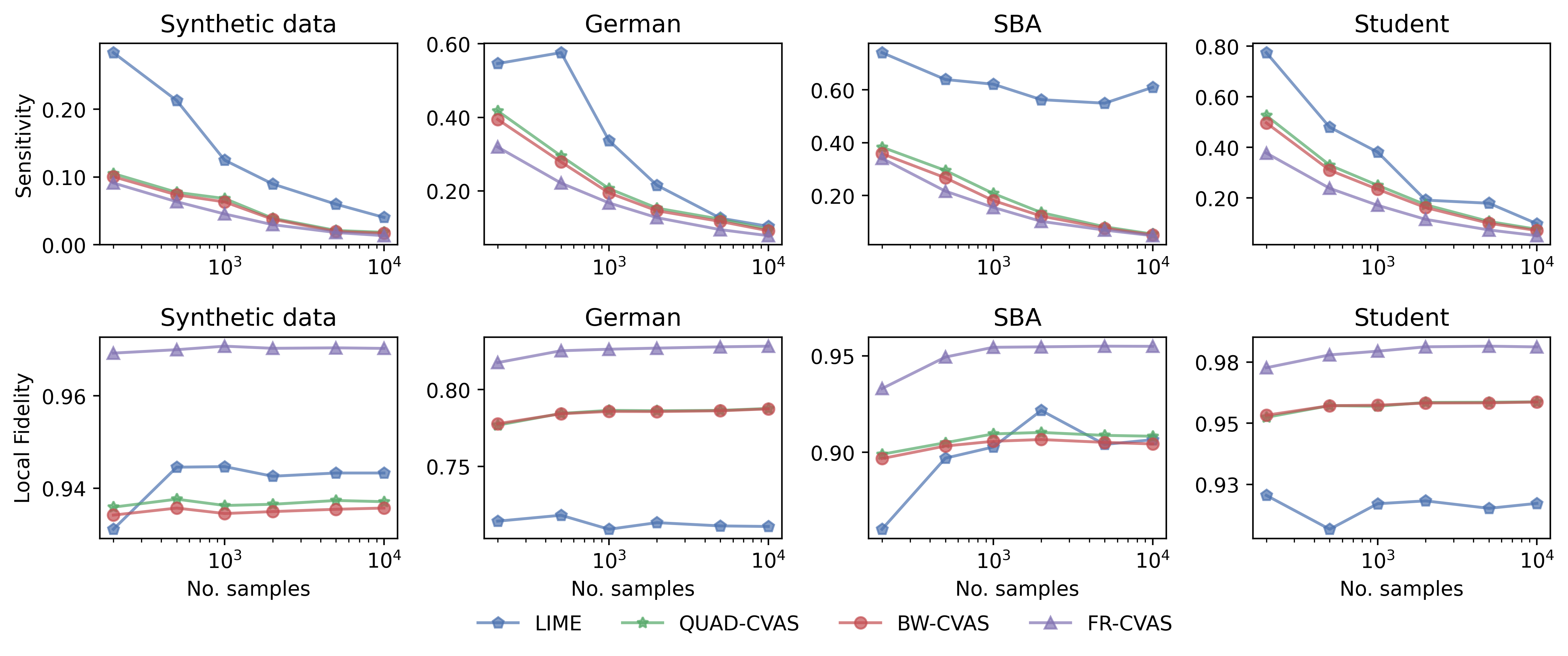
Figure 6. Benchmarks of sensitivity (top row) and local fidelity (bottom row) on four datasets. Lower sensitivity and higher local fidelity are better.

Sensitivity. We use the procedure in [1] to measure the sensitivity of the surrogates with respect to small perturbations in the input instance. For a given instance $x$, we draw a set $\mathcal{U}_{x}$ of 10 neighbors of $x$ from $\mathcal{N}(x,0.001I)$ independently. We use the above-mentioned methods to find the linear surrogate $\theta_{x^{\prime}}=(w_{x^{\prime}},b_{x^{\prime}})$ for each $x^{\prime}\in\mathcal{U}_{x}$. We report the maximum difference between the surrogates for $x^{\prime}$ and that for $x$. Precisely, the sensitivity of a surrogate $\theta_{x}$ can be computed by

$$\mathrm{Sensitivity}(\theta_{x})=\max\nolimits_{x^{\prime}\in\mathcal{U}_{x}}\|w_{x}-w_{x^{\prime}}\|_{2}.$$

Ideally, the smaller the sensitivity, the better because it indicates that the surrogate is more stable to perturbations in the input instance $x_{0}$.

Local Fidelity. We use the $\mathrm{LocalFid}$ criterion as in [32] to measure the fidelity of a local surrogate model to the underlying model. For a given instance $x$ and a constructed linear surrogate $\mathcal{C}_{\theta_{x}}$, we draw a set $\mathcal{V}_{x}$ of 1000 instances uniformly from an $l_{2}$-ball of radius $r_{\mathrm{fid}}$ centered on $x$. The local fidelity of the surrogate $\theta_{x}$ is then measured as:

$$\mathrm{LocalFid}(\theta_{x})=\frac{1}{2|\mathcal{V}_{x}|}\sum_{x^{\prime}\in\mathcal{V}_{x}}\left|f(x^{\prime})-\mathcal{C}_{\theta_{x}}(x^{\prime})\right|,$$

where $f$ is the original classifier. The metric $\mathrm{LocalFid}$ measures the fraction of instances where the output class of $f$ and $\mathcal{C}_{\theta_{x}}$ agree. The constant $2$ in the denominator normalizes the value to $[0,1]$ because the output of the models is in $\{-1,+1\}$. The higher local fidelity value indicates that the linear surrogate $\mathcal{C}_{\theta_{x}}$ better approximates the local decision boundary of $f$. Here, we set $r_{\mathrm{fid}}$ to 10$\%$ of the maximum distance between instances in the training data. Note that $\mathcal{V}_{x}$ is for evaluation only and independent from the perturbation samples used to train the local surrogate.

To construct our CVASes, we choose $k=10$ examples in the favorable class with the smallest $\ell_{1}$ distance to the input instance $x_{0}$. We then use these examples to perform a line search to find $x_{b}$. The perturbation radius $r_{p}$ is set to 5% of the maximum distance between instances in the training data and set $\rho_{+1}=0$, $\rho_{-1}=1.0$. For LIME, we use the default parameters recommended in the LIME source code and return $\theta=(w,b-0.5)$ as the LIME’s surrogate, similar to [32]. We vary the number of perturbation samples in a range of $[500,10000]$ to measure the fidelity and sensitivity of constructed surrogates under small sampling sizes. The results in Figure 6 show the superiority of CVASes to LIME in both sensitivity and local fidelity metrics. Meanwhile, FR-CVAS provides higher-fidelity surrogates compared to QUAD-CVAS and BW-CVAS. These results assert that CVAS variants can serve as competitive linear surrogates to approximate the nonlinear decision boundary of black-box classifiers. The family of (covariance-robust) CVASes thus possesses a great opportunity to be an algorithmic explainer. However, we will focus on integrating CVASes into the recourse generation workflow for the remainder of the experiments.

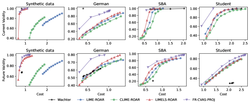
Figure 7. Pareto frontier of the cost-validity trade-off on four datasets. Each method has 11 configurations for the ambiguity size, but only non-dominated configurations are presented for clarity.

6.2. CVAS for Robust Recourse Generation

We now study the integration of the covariance-robust CVASes into the recourse generation scheme and the related robustness to model shifts and the cost-validity trade-off. Proposition 5.2 suggests that the Fisher-Rao model is a good candidate to form the surrogate for the recourse generation. In this section, we use FR-CVAS as the linear surrogate $\theta^{\mathds{F}}=(w^{\mathds{F}},b^{\mathds{F}})$, and we integrate $\theta^{\mathds{F}}$ with two types of generation: gradient-based recourse method (Section 6.2.1) and actionable recourse method (Section 6.2.2). Notice that $\theta^{\mathds{F}}$ inherently depends on the ambiguity size $\rho$, but this dependence is omitted to avoid clutter.

Metrics. Throughout this experiment, we use an $\ell_{1}$-distance as the cost function, which is a standard setting in the literature [62, 61]. We define the current validity as the validity of the generated recourses with respect to the given black-box classifier. To measure the validity of recourses under the model shifts, we sample $80\%$ instances of the shifted data $D_{2}$ 100 times to train 100 ‘future’ MLP classifiers. We then report the future validity of recourse as the fraction of the future classifiers with respect to which the recourse remains valid. Both the current and future validity are standard metrics in the literature of robust recourse [61, 40].

6.2.1. Robust Projection-based Recourse

Because CVAS is a linear surrogate, the most simple recourse search is a projection onto the decision boundary surrogate. We thus consider the following recourse search mechanism

$$x_{r}=\arg\min\{\|x-x_{0}\|_{1}:x^{\top}w^{\mathds{F}}+b^{\mathds{F}}\geq 0\},$$

which is the 1-norm projection onto the hyperplane $\{x:x^{\top}w^{\mathds{F}}+b^{\mathds{F}}\geq 0\}$. This method is named FR-CVAS-PROJ. We compare this simple recourse against several baselines:

1. Wachter [68] (Wachter). We suppose that the binary classifier $f$ takes the form

   $$f(x)=\begin{cases}+1&\text{if }g(x)\geq 0.5,\\ -1&\text{otherwise,}\end{cases}$$

   where $g(x)$ is the probability output of the model. Then Wachter solves

   (6.1) $$\min\limits_{x}~{}\left\{(g(x)-0.5)^{2}+\lambda\|x-x_{0}\|_{1}\right\},$$

   where the first term is a quadratic loss function between the probability output of $x$ and the threshold $0.5$, and the second term is the $\ell_{1}$-distance between $x$ and $x_{0}$. The parameter $\lambda>0$ is the weight balancing the validity and the implementation cost. We use a well-known CARLA’s implementation for Wachter [68]. This repository employs an adaptive scheme to adjust the hyperparameter $\lambda$ if no valid recourse is found.

2. a simple 1-norm projection onto the LIME surrogate (LIME-PROJ),

3. a min-max formulation ROAR [61] coupled with three local surrogates LIME [50], CLIME [1], and LIMELS [32] as nominal surrogate (LIME-ROAR, CLIME-ROAR, and LIMELS-ROAR, respectively). While LIME trains a weighted linear regression, CLIME trains a linear regression, and LIMELS trains a ridge regression to find the surrogate. Because there is no publicly available implementation for CLIME [1] and LIMELS [32], we implement according to the original papers and based on LIME’s source code. We use the CARLA’s implementation for ROAR and set the initial $\lambda$ to $0.1$ as suggested in [61].

Note, once again, that Wachter and LIME-PROJ are simple gradient-based methods that are not necessarily robust, while ROAR is a robust method using a min-max formulation.

Table 1. Performance of competing algorithms on the German, SBA, and Student datasets. For the current and future validity, higher is better. For the cost, lower is better. Bold indicates the best performance. FR-CVAS-PROJ has similar future validity to ROAR-related methods but has higher current validity and lower cost.

Method	German			SBA			Student
	Cost $\downarrow$	Cur Validity $\uparrow$	Fut Validity $\uparrow$	Cost $\downarrow$	Cur Validity $\uparrow$	Fut Validity $\uparrow$	Cost $\downarrow$	Cur Validity $\uparrow$	Fut Validity $\uparrow$
Wachter	0.44 $\pm$ 0.03	1.00 $\pm$ 0.00	0.53 $\pm$ 0.03	1.15 $\pm$ 0.15	0.97 $\pm$ 0.01	0.14 $\pm$ 0.06	2.30 $\pm$ 0.04	0.95 $\pm$ 0.03	0.31 $\pm$ 0.04
LIME-PROJ	0.45 $\pm$ 0.10	0.35 $\pm$ 0.11	0.51 $\pm$ 0.08	0.81 $\pm$ 0.06	0.97 $\pm$ 0.01	0.79 $\pm$ 0.03	1.07 $\pm$ 0.13	0.78 $\pm$ 0.04	0.37 $\pm$ 0.07
LIME-ROAR	1.09 $\pm$ 0.19	0.66 $\pm$ 0.15	0.64 $\pm$ 0.08	1.83 $\pm$ 0.16	1.00 $\pm$ 0.00	0.87 $\pm$ 0.04	2.41 $\pm$ 0.31	0.95 $\pm$ 0.03	0.74 $\pm$ 0.11
CLIME-ROAR	1.40 $\pm$ 0.45	0.76 $\pm$ 0.17	0.72 $\pm$ 0.11	1.50 $\pm$ 0.53	0.97 $\pm$ 0.04	0.78 $\pm$ 0.13	3.07 $\pm$ 0.75	0.95 $\pm$ 0.04	0.81 $\pm$ 0.11
LIMELS-ROAR	1.29 $\pm$ 0.07	0.88 $\pm$ 0.03	0.79 $\pm$ 0.02	1.63 $\pm$ 0.23	1.00 $\pm$ 0.00	0.88 $\pm$ 0.05	2.47 $\pm$ 0.29	0.95 $\pm$ 0.03	0.75 $\pm$ 0.09
FR-CVAS-PROJ	1.04 $\pm$ 0.02	0.94 $\pm$ 0.03	0.79 $\pm$ 0.01	1.72 $\pm$ 0.13	1.00 $\pm$ 0.00	0.97 $\pm$ 0.02	2.34 $\pm$ 0.20	0.95 $\pm$ 0.03	0.80 $\pm$ 0.06

The main comparison herein is the cost-validity trade-off among different methods. We fix the number of perturbation samples to $1000$ and vary the ambiguity size with $\rho_{+1}=0$, $\rho_{-1}\in[0,10]$ with step size $0.1$ for FR-CVAS-PROJ, and $\delta_{\max}\in[0,0.2]$ with step size $0.02$ for the uncertainty size of ROAR. We then plot the Pareto frontiers of the cost-validity trade-off in Figure 7. Generally, increasing the ambiguity size $\rho$ will increase the current and future validity of the FR-CVAS-PROJ recourse, but will also sacrifice in terms of the implementation cost. A similar observation applies to ROAR-related recourses when we increase the uncertainty size $\delta_{\max}$. These results are consistent with the analysis in [49]. However, the Pareto frontiers of FR-CVAS-PROJ dominate the frontiers of ROAR-related methods on all evaluated datasets. In other words, with the same cost (or validity), our method will provide recourses with a higher validity (or lower cost) compared to ROAR. For the experiment in Table 1, we choose $\rho_{+1}=0,\rho_{-1}=10$ for FR-CVAS-PROJ and $\delta_{\max}=0.2$ for ROAR with different surrogates. Table 1 demonstrates that our method has similar validity but a much smaller cost than the best baseline LIMELS-ROAR on German datasets. Meanwhile, our method achieves higher validity with reasonable cost on SBA and Student datasets.

6.2.2. Robust Actionable Recourse

Because our proposed covariance-robust CVASes can explicitly hedge against model shifts, our method can be integrated with AR [62] to promote robust and actionable recourses. To ensure that recourses are actionable, AR restricts each feature to a discrete set of feasible values predefined using the training data. We follow the specification in [62] and model the actionability using mixed-integer constraints. The robust actionable recourse is

$$x_{ar}=\arg\min\{\|x-x_{0}\|_{1}:x^{\top}w^{\mathds{F}}+b^{\mathds{F}}\geq 0,~{}\delta=x-x_{0},~{}\delta\text{~{}actionable}\}.$$

Here, each feature $\delta_{j}$ is restricted to a grid of $m_{j}+1$ feasible values $\delta_{j}\in\{0,\delta_{j1},\ldots,\delta_{jm_{j}}\}$ via the indicator variables. Following the same setup in [46], we consider the actionability constraints such as immutable race, gender, or non-decrease age; see Appendix A.1 for the specification of the actionability constraints. We use the original authors’ implementations of for AR.

For the baselines, we will compare our above robust actionable recourse against three different surrogates, where $(w^{\mathds{F}},b^{\mathds{F}})$ are replaced by the LIME, CLIME, and LIMELS, respectively. For FR-CVAS, we set $\rho_{+1}=0$, $\rho_{-1}=1.0$. Table 2 demonstrates that the actionable recourse with FR-CVAS surrogate increases the current and future validity substantially compared to other surrogates.

Table 2. Performance of AR using different local surrogates.

Method	German			SBA			Student
	Cost $\downarrow$	Cur Validity $\uparrow$	Fut Validity $\uparrow$	Cost $\downarrow$	Cur Validity $\uparrow$	Fut Validity $\uparrow$	Cost $\downarrow$	Cur Validity $\uparrow$	Fut Validity $\uparrow$
LIME-AR	0.44 $\pm$ 0.08	0.14 $\pm$ 0.05	0.39 $\pm$ 0.07	4.76 $\pm$ 3.06	0.09 $\pm$ 0.06	0.05 $\pm$ 0.03	3.38 $\pm$ 0.25	0.46 $\pm$ 0.07	0.42 $\pm$ 0.06
CLIME-AR	0.72 $\pm$ 0.52	0.27 $\pm$ 0.12	0.44 $\pm$ 0.10	5.73 $\pm$ 4.13	0.40 $\pm$ 0.38	0.17 $\pm$ 0.18	4.35 $\pm$ 1.24	0.63 $\pm$ 0.28	0.49 $\pm$ 0.15
LIMELS-AR	0.36 $\pm$ 0.11	0.24 $\pm$ 0.09	0.44 $\pm$ 0.08	5.48 $\pm$ 3.17	0.19 $\pm$ 0.07	0.07 $\pm$ 0.04	3.16 $\pm$ 0.16	0.49 $\pm$ 0.13	0.38 $\pm$ 0.03
FR-CVAS-AR	1.95 $\pm$ 0.11	0.80 $\pm$ 0.05	0.73 $\pm$ 0.03	7.59 $\pm$ 2.42	0.83 $\pm$ 0.18	0.50 $\pm$ 0.21	9.64 $\pm$ 0.38	1.00 $\pm$ 0.00	0.95 $\pm$ 0.03

7. Conclusions

This paper developed a new framework of robust recourse design, with the flexibility to incorporate additional mixed-integer constraints for capturing various practical considerations. One notable feature of our framework is a novel linear surrogate for approximating the nonlinear decision boundary of a black-box machine learning model, called the coverage-validity-aware surrogate. The proposed surrogate allows us to trade off the two criteria, coverage and validity, in a geometrically intuitive manner. Theoretically, we established the strong connections between this surrogate and the canonical MPM classifier. Moreover, we studied multiple robust variants, which are able to hedge against boundary shifts. We showed that these robust variants correspond to new forms of regularizations of the MPM classifier. We have investigated the asymptotic properties of the robust variants of the proposed surrogate. Through extensive numerical results with using real datasets, we demonstrated that our surrogates exhibit higher fidelity to the underlying model and lower sensitivity to the problem inputs compared to well-known baseline surrogates. Consequentially, our recourses achieved robustness with a better cost-validity trade-off while enabling actionability through mixed-integer constraints.

Appendix A Additional Experiments

A.1. Experimental Details

Synthetic data generation. For synthetic data, we generate 2-dimensional data by sampling instances uniformly in a rectangle $x=(x_{1},x_{2})\in[-2,4]\times[-2,7]$. Each sample is labeled using the following function:

$$f(x)=\left\{\begin{array}[]{cl}1&\mathrm{if}\quad x_{2}\geq 1+x_{1}+2x_{1}^{2}+x_{1}^{3}-x_{1}^{4}+\varepsilon,\\ -1&\mathrm{otherwise},\end{array}\right.$$

where $\varepsilon$ is a random noise. We generate a present data set $D_{1}$ with $\varepsilon=0$ and a shifted data set $D_{2}$ with $\varepsilon\sim\mathcal{N}(0,1)$. The decision boundary of the MLP classifier for current synthetic data is illustrated in Figure 8.

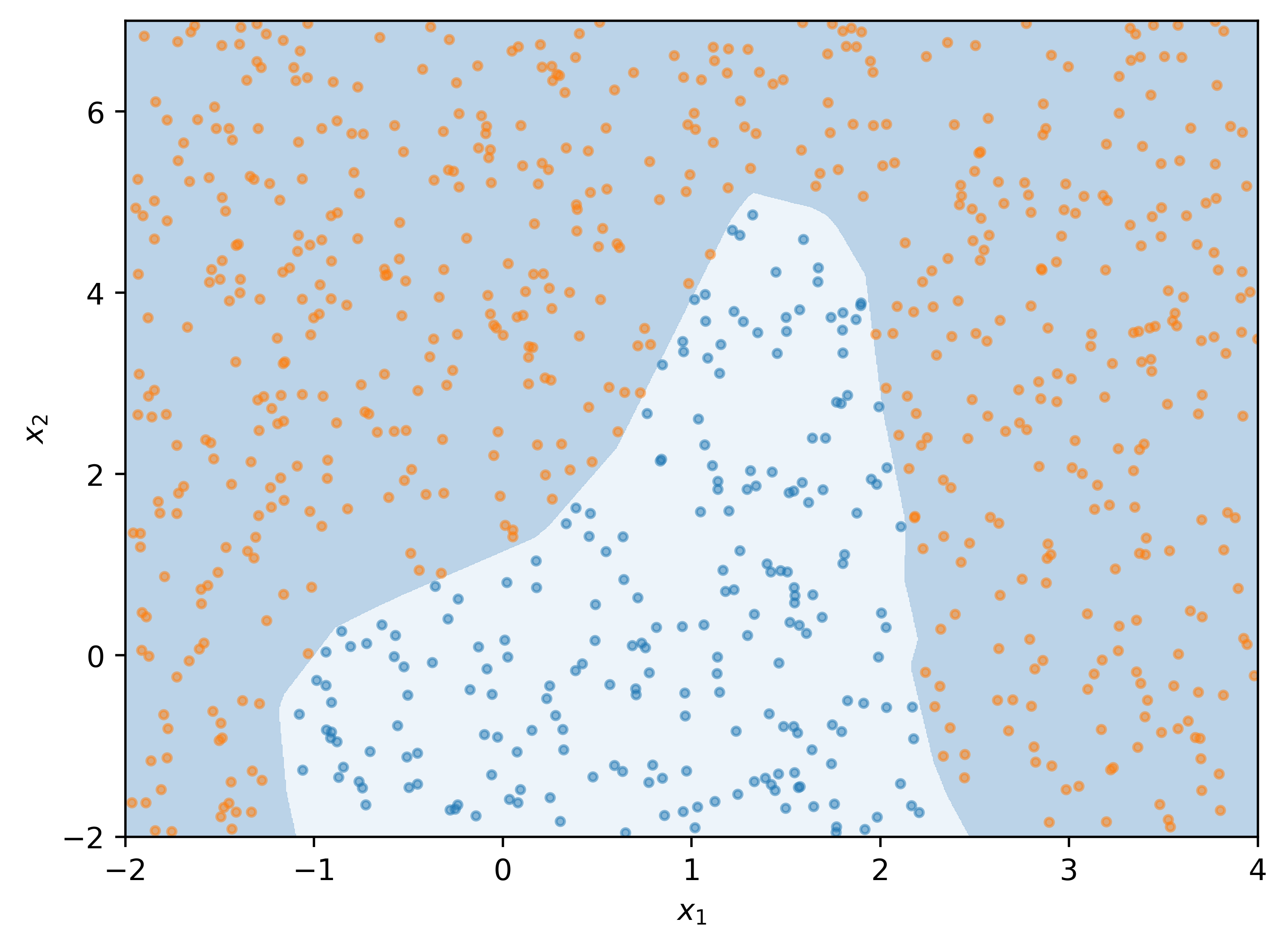
Figure 8. An illustration of MLP’s decision boundary for the synthetic data.

Real-world datasets. The details of three real-world datasets are listed below:

1. German Credit [16]. The dataset contains the information (e.g. age, gender, financial status,…) of 1000 customers who took a loan from a bank. The classification task is to determine an individual’s risk (good or bad). There is another version of this dataset regarding corrections of coding error [21]. We use the corrected version of this dataset as shifted data to capture the correction shift. The features we used in this dataset include ‘duration’, ‘amount’, ‘personal_status_sex’, and ‘age’. When considering actionability constraints in Section 6.2, we set ‘personal_status_sex’ as immutable and ‘age’ to be non-decreasing.

2. Small Bussiness Administration (SBA) [34]. This data includes 2,102 observations with historical data of small business loan approvals from 1987 to 2014. We divide this dataset into two datasets (one is instances from 1989 - 2006 and one is instances from 2006 - 2014) to capture temporal shifts. We use the following features: selected, ‘Term’, ‘NoEmp’, ‘CreateJob’, ‘RetainedJob’, ‘UrbanRural’, ‘ChgOffPrinGr’, ‘GrAppv’, ‘SBA_Appv’, ‘New’, ‘RealEstate’, ‘Portion’, ‘Recession’. When considering actionability constraints, we set ‘UrbanRural’ as immutable.

3. Student performance [13]. This data includes the performance records of 649 students in two schools: Gabriel Pereira (GP) and Mousinho da Silveira (MS). The classification task is to determine whether their final score is above average. We split this dataset into two sets in two schools to capture geospatial shifts. The features we used are: ‘age’, ‘Medu’, ‘Fedu’, ‘studytime’, ‘famsup’, ‘higher’, ‘internet’, ‘romantic’, ‘freetime’, ‘goout’, ‘health’, ‘absences’, ‘G1’, ‘G2’. When considering actionability constraints, we set ‘romantic’ as immutable and ‘age’ to be non-decreasing.

For categorical features, we convert them to binary features using the same one-hot encoding procedure proposed by [38]. We also normalize continuous features to zero mean and unit variance before training the classifier. The classifier’s performance on all datasets is reported in Table 3.

Table 3. Accuracy and AUC results of the classifiers on the synthetic and three real-world datasets.

Classifier	Dataset	Present data $D_{1}$		Shift data $D_{2}$
		Accuracy $\uparrow$	AUC $\uparrow$	Accuracy $\uparrow$	AUC $\uparrow$
MLP	Synthetic data	0.99 $\pm$ 0.00	1.00 $\pm$ 0.00	0.94 $\pm$ 0.01	0.99 $\pm$ 0.01
	German credit	0.67 $\pm$ 0.02	0.60 $\pm$ 0.03	0.66 $\pm$ 0.23	0.60 $\pm$ 0.04
	SBA	0.96 $\pm$ 0.00	0.99 $\pm$ 0.00	0.98 $\pm$ 0.01	0.96 $\pm$ 0.01
	Student	0.86 $\pm$ 0.02	0.93 $\pm$ 0.01	0.91 $\pm$ 0.04	0.97 $\pm$ 0.02

Reproducibility. We release all source code and scripts to replicate our experimental results at https://anonymous.4open.science/r/cvas. The repository includes source code, datasets, configurations, and instructions.

The hyperparameter configurations for our methods and other baseline are clearly stated in Section 6, Appendix A.1 and Appendix A.2 and also stored in the repository. The surrogates sharing the same local sampler have the same random seed and, therefore, have the same synthesized samples. The hyperparameters that affect baselines’ performance such as $\lambda$ and the probabilistic threshold of Wachter and ROAR will also be studied in Appendix A.2.

A.2. Additional Experimental Results

A.2.1. Local Fidelity and Sensitivity Comparisons

We run with a different setting for the sensitivity and local fidelity metric to assess the sensitivity of the results to the parameter choices. Specifically, we sample 10 neighbors in the distribution $\mathcal{N}(x,0.0001I)$ instead of $\mathcal{N}(x,0.001I)$ to measure the sensitivity. Meanwhile, we set $r_{fid}$ to 20% and the radius $r_{p}$ to 10% of the maximum distance between training instances. The result in Figure 9 is consistent with Figure 6, showing that our evaluation is not sensitive to the choice of hyper-parameters used to compute the metrics.

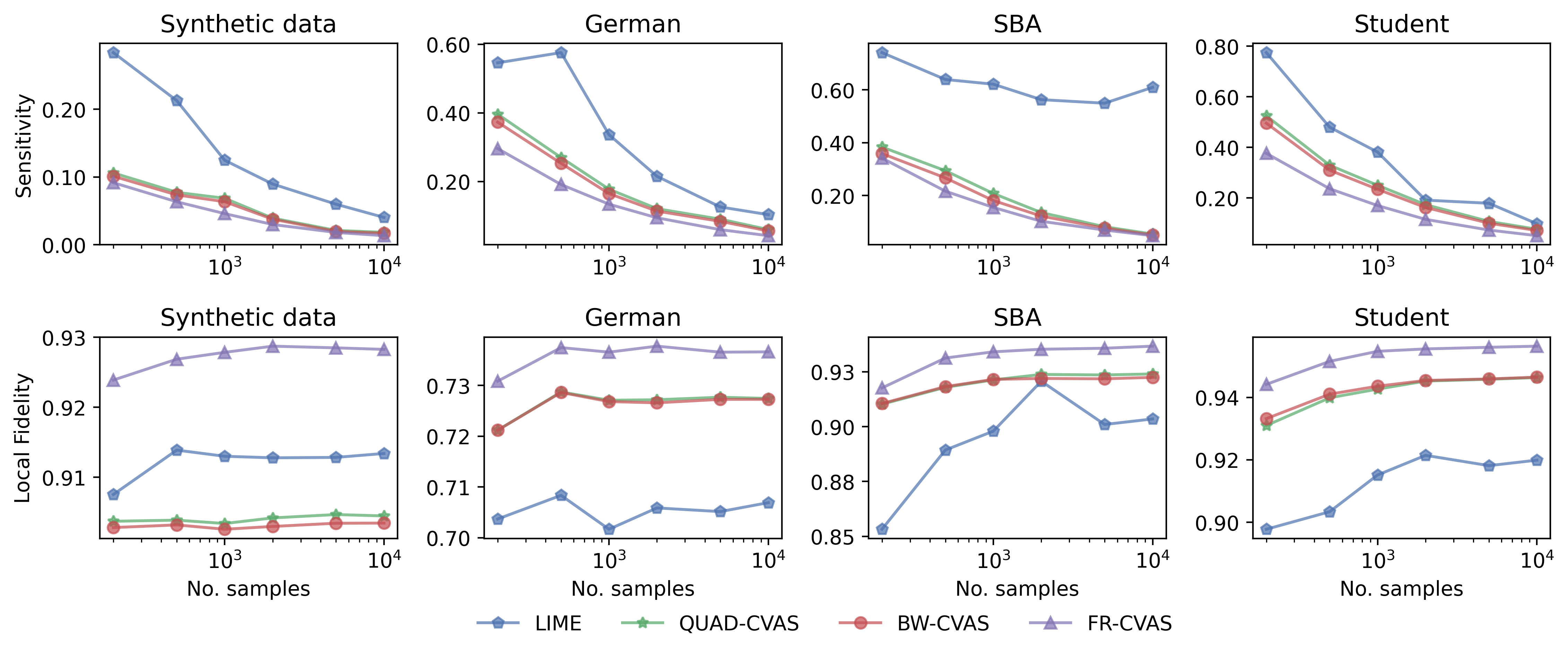
Figure 9. Benchmarks of sensitivity and local fidelity of LIME and CVAS variants on four datasets.

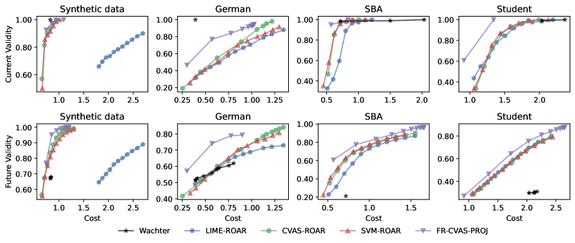
Figure 10. Pareto frontiers of our method compared with ROAR using LIME, non-robust CVAS, and SVM as the surrogate model. The recourses are generated with respect to the MLP classifier on synthetic and three real-world datasets.

A.2.2. Comparison with ROAR using the non-robust CVAS and SVM as the surrogate model.

Here, we compare the FR-CVAS-PROJ with ROAR using LIME, vanilla CVAS, and SVM [25] as the surrogate model. Both vanilla CVAS and SVM use the same boundary sample procedure (with the same seed number) as FR-CVAS. The settings are similar to the experiment in Section 6.2. The result shown in Figure 10 demonstrates the merits of our method.

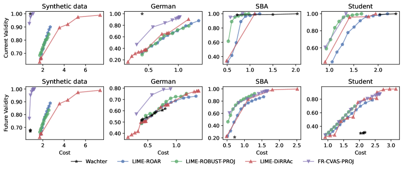
Figure 11. Ablation study: Pareto frontiers of FR-CVAS-PROJ compared to its ablations by alternating the FR-CVAS by LIME and alternating ROAR by DiRRAc and the robust projection. The recourses are generated with respect to the MLP classifier on synthetic and three real-world datasets.

A.2.3. Ablation Study.

We conduct an ablation study to understand the contribution of local surrogate models and recourse-generation approaches in our method. Figure 10 shows the comparison of our method with ROAR using vanilla CVAS and SVM as the local surrogate. Figure 11 shows the Pareto frontiers of FR-CVAS-PROJ compared to its ablations by substituting the FR-CVAS with other surrogates (LIME, CVAS) or substituting ROAR [61] by DiRRAc [40]. We also compare our method with LIME-ROBUST-PROJ, which uses LIME as the surrogate model and then solves the robustified projection:

$$x_{r}=\arg\min\{\|x-x_{0}\|_{1}~{}:~{}x\in\mathbb{R}^{d},~{}x^{\top}w+b-\delta_{\mathrm{max}}\|x\|_{2}\geq 0\},$$

where $(w,b)$ is the weight and bias of the LIME’s surrogate and $\delta_{\mathrm{max}}$ is similar to the uncertainty size of ROAR [61].

The recourses are generated with respect to the MLP classifier on synthetic and three real-world datasets. This result demonstrates the usefulness of the FR-CVAS in promoting the generation of robust recourses. Note that, for $\rho_{-1}=0$ and $\rho_{+1}=0$, the hyperplane of the FR-CVAS classifier coincides with the vanilla CVAS’s hyperplane.

A.2.4. Comparison with the Probabilistic Threshold Shiftings.

A probabilistic classifier uses a threshold to convert the probability to a binary outcome: if the probability value is above the threshold value, the outcome is considered ‘favorable’ (class $+1$). The standard threshold is 0.5, that is used as in Equation (6.1), and one possible approach to generate robust recourse is simply running the recourse generation problem with the same black-box classifier but with a higher threshold value. In doing so, the recourse will have a higher probability of being classified in the $+1$ class with respect to the current classifier. This can hopefully be translated to a higher probability of being classified in the $+1$ class with respect to the future classifier. While this method may not provide any guarantee, it is a simple and intuitive baseline.

In Figure 12, we compare the proposed method with Wachter, LIME, and vanilla CVAS with various probabilistic thresholds in the range $[0.5,0.9]$. For vanilla CVAS, we first obtain the solution $\widehat{\theta}=(\widehat{w},\widehat{b})$ for the coverage-validity-aware surrogate problem (2.3) and calibrate the intercept $\widehat{b}$. Figure 12 demonstrates that FR-CVAS-PROJ consistently achieves the best performance compared to other baselines. Interestingly, Wachter improves its future validity significantly on the synthetic and German datasets as the threshold increases. However, our method still dominates Wachter in all datasets. These results also suggest that robustification via distributionally robust optimization is more effective than that via the calibration of linear surrogate thresholds.

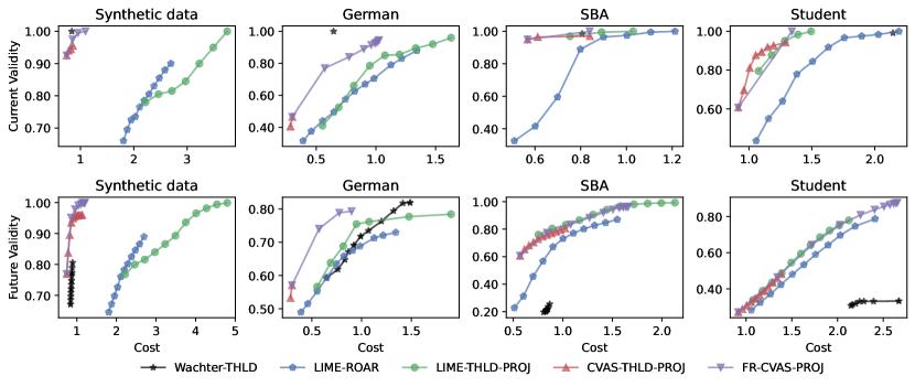
Figure 12. Comparison of FR-CVAS-PROJ, LIME-ROAR, and the probabilistic shiftings (Wachter-THLD, LIME-THLD-PROJ and CVAS-THLD-PROJ).

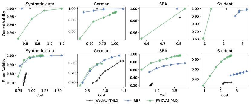
Figure 13. Comparison of our FR-CVAS-PROJ against RBR. We also plot Wachter with threshold shiftings as a comparison in the plot.

A.2.5. Comparison with Model Agnostic Approaches

We also compare FR-CVAS-PROJ with Robust Bayesian Recourse (RBR), a model-agnostic approach [41]. RBR does not use a surrogate model; instead, it directly optimizes the quasi-likelihood of the recourse using the synthesized samples. The frontiers for RBR are obtained by varying $\delta_{+}\in[0,0.2]$ and $\varepsilon_{1}\in[0,1.0]$. Figure 13 shows that FR-CVAS-PROJ provides a better cost-validity trade-off than RBR, especially on SBA and Student datasets.

A.2.6. Robust CVASes with Different Divergences

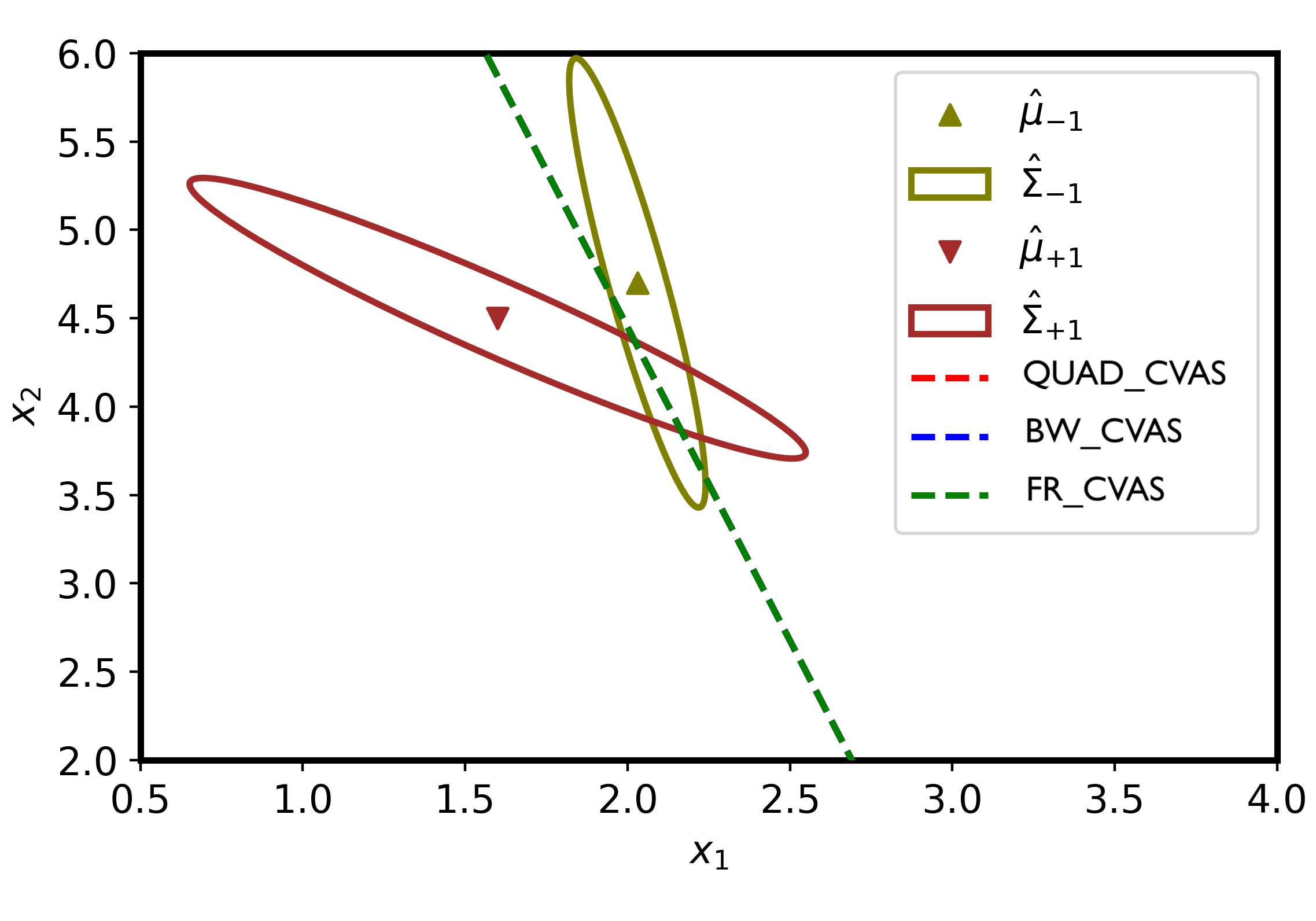
(a) $\rho_{+1}=\rho_{-1}=0$.

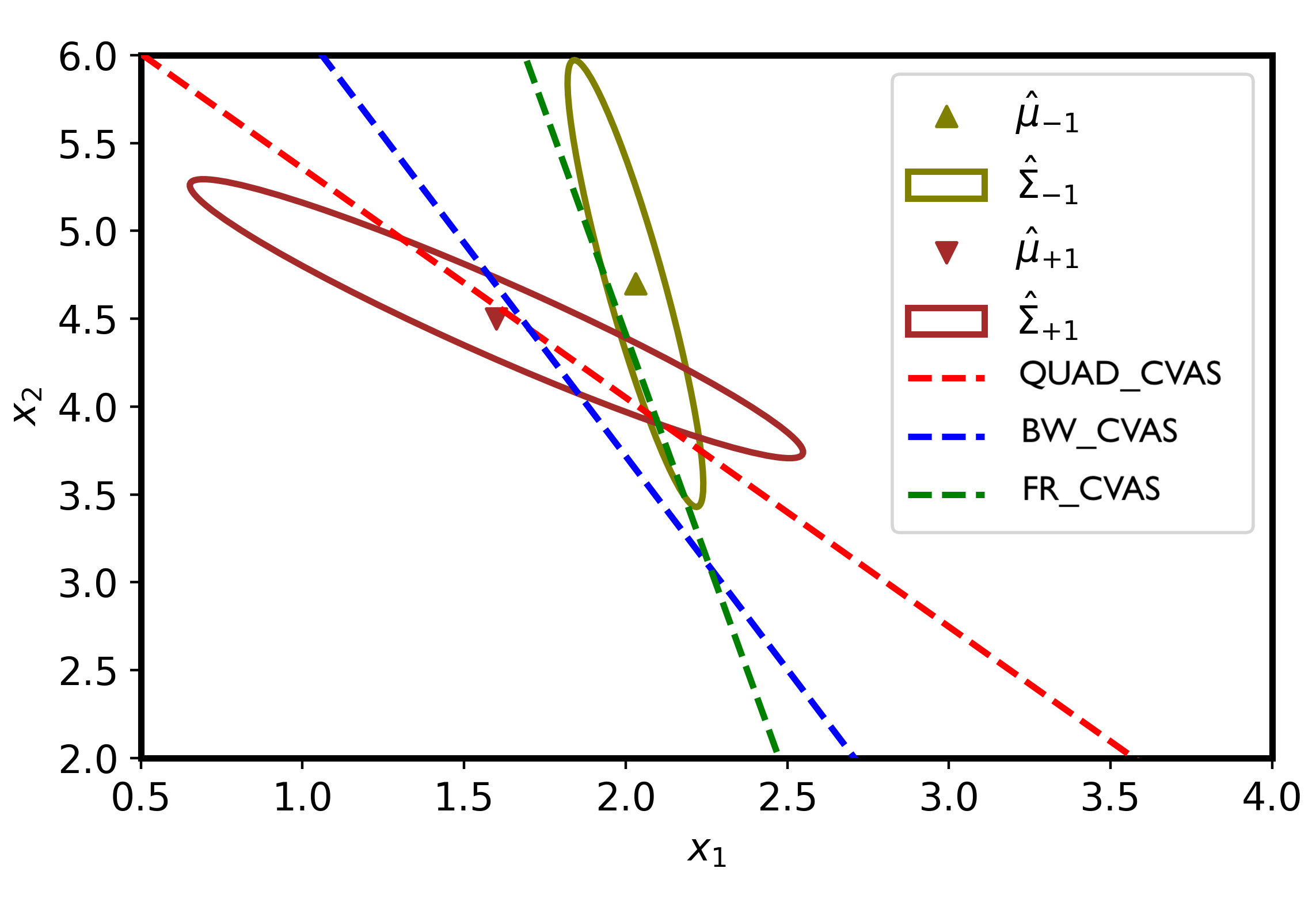
(b) $\rho_{+1}=0,\rho_{-1}=1$.

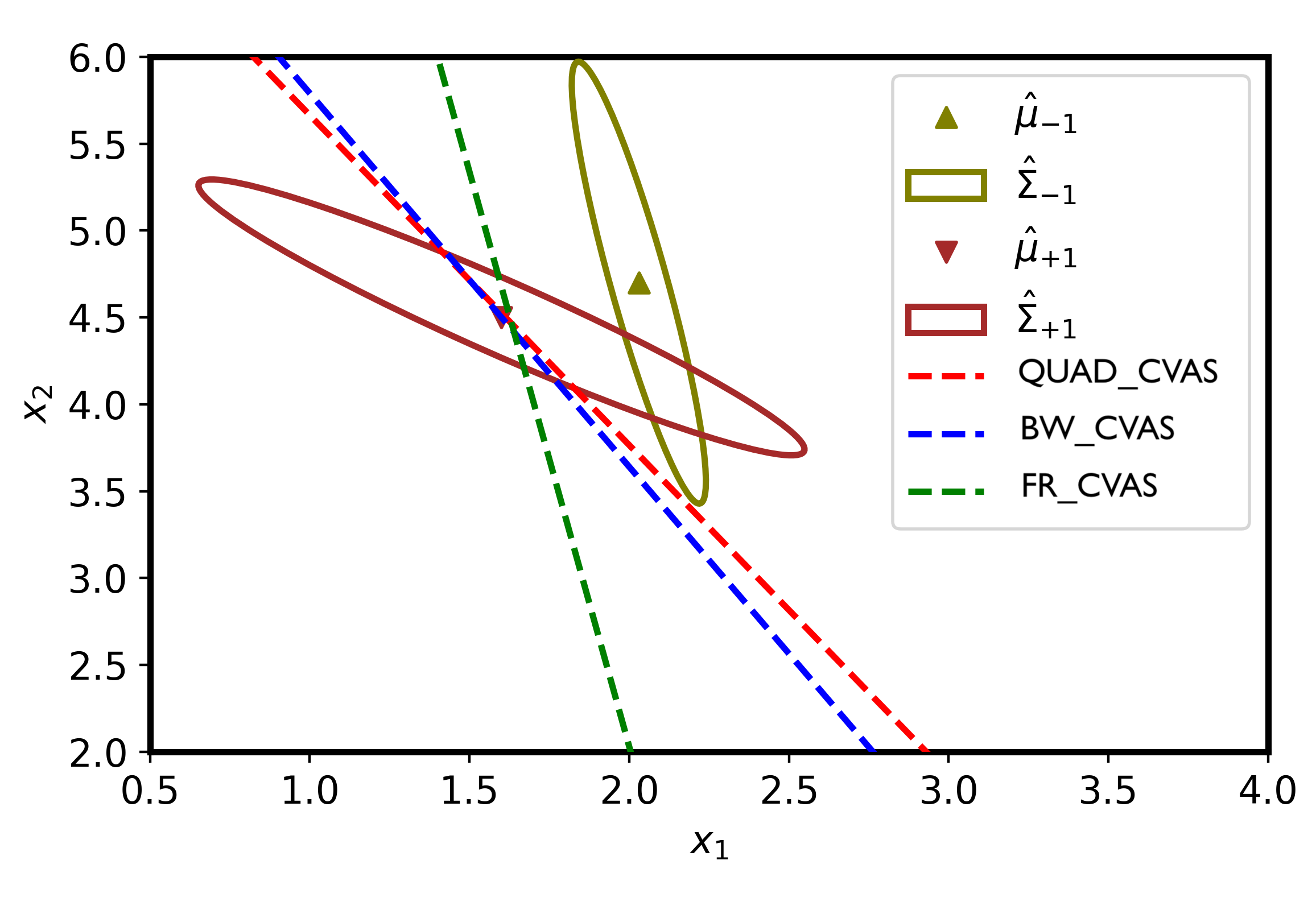
(c) $\rho_{+1}=0,\rho_{-1}=10$.

Figure 14. Visualization of CVAS’s hyperplanes with Quadratic, Bures, and Fisher-Rao distances.

This section discusses the variants of covariance-robust CVASes with different divergences. This discussion aims to provide guidance for choosing the surrogate model in practice, especially at a low sample size.

Proposition 5.1 showed that Quadratic surrogate and Bures surrogate coincide when one of the radii $\rho_{y}$ grows to infinity, and they are independent of the covariance matrices $\widehat{\Sigma}_{y}$. Meanwhile, the asymptotic hyperplane of the Fisher-Rao surrogate when $\rho_{y}\to\infty$ aligns with axes of the covariance matrices $\widehat{\Sigma}_{y}$ (see Proposition 5.1 and Figure 14). We can observe that when $\rho_{+1}=\rho_{-1}=0$, all hyperplanes coincide and recover the non-robust CVAS. All hyperplanes move towards the favorable class as the radius for the unfavorable class $\rho_{-1}$ increases. At $\rho_{-1}=10$ in Subfigure 14(c), the hyperplanes of the Quadratic and Bures surrogates come close together, which is distinct from the Fisher-Rao hyperplane. Notice that the Fisher-Rao surrogate in Subfigure 14(c) tends to position in parallel to the major axis of the unfavorable covariance matrix, which shows the dependence on $\widehat{\Sigma}_{-1}$. The Bures and Quadratic hyperplanes in Subfigure 14(c) do not depend on the covariance matrix, which aligns with the results in Proposition 5.1. Coupled with Proposition 5.2, we postulate that the Fisher-Rao surrogate is not a suitable surrogate at low sample sizes as it relies on the estimate of the covariance matrices. On the other hand, when the number of samples is sufficient to estimate the covariance matrices accurately, the Fisher-Rao surrogate would be better than the Quadratic and Bures surrogate as it considers the geometry of the data during robustification.

We probe the performance of CVASes with different divergences at low sample sizes to demonstrate our claim above.

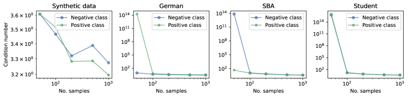
(a) The average condition number of the generated covariance matrices for positive and negative classes.

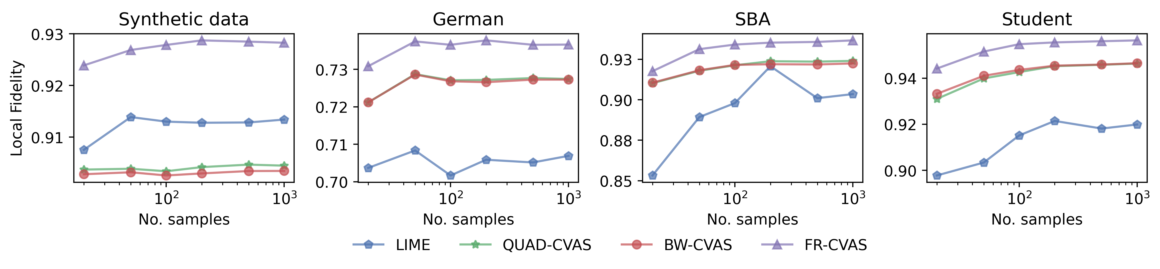
(b) Local fidelity of CVAS variants at low sample sizes.

Figure 15. The comparison among CVAS variants with different distances at low sample sizes.

Local fidelity. We probe the local fidelity at low sample sizes and plot the result in Figure 15. The experiment settings are similar to those in Section 6.1. The number of samples is set in the range of $[50,1000]$. We also measure the average condition number of estimated covariance matrices for both positive and negative classes in Figure 15(a). This figure shows that the covariance matrices are ill-conditioned at 50 samples on SBA and Student datasets. The fidelity of FR-CVAS is just slightly better than QUAD-CVAS and BW-CVAS. When the number of samples increased, FR-CVAS benefited the most, and the gap between FR-CVAS and QUAD-CVAS (or BW-CVAS) became more significant. It supports our claim that FR-CVAS would better approximate the decision boundary when the number of samples is sufficient for estimating the covariance matrices.

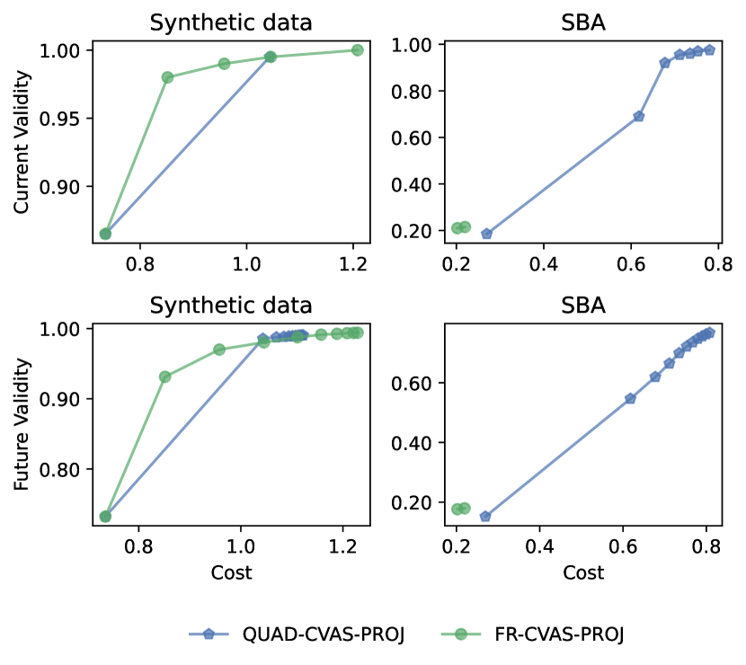
(a) 50 synthesized samples.

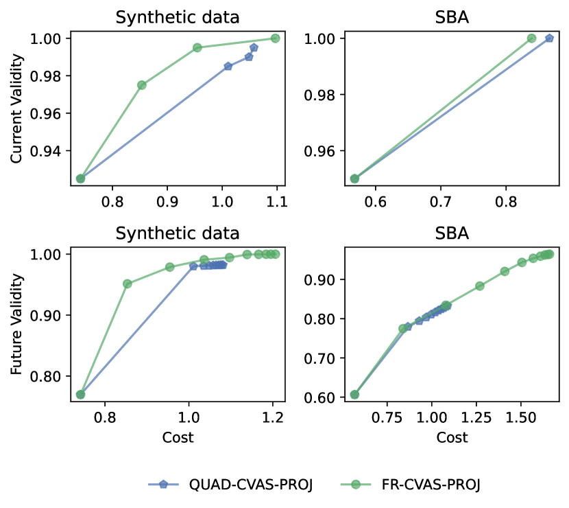
(b) 1000 synthesized samples.

Figure 16. The comparison of QUAD-CVAS-PROJ and FR-CVAS-PROJ at different sample sizes.

Robust recourses. We revisit the recourse generation with covariance-robust CVASes using Quadratic distance (QUAD-CVAS-PROJ) and Fisher-Rao distance (FR-CVAS-PROJ), at which the surrogate is estimated with 50 and 1000 synthesized samples. We omit the comparison with Bures distance to ease the presentation as it behaves asymptotically like the Quadratic surrogate. The results are shown in Figure 16. The results showed that QUAD-CVAS-PROJ would be better at low sample size. When increasing the number of samples, the recourses constructed with the Fisher-Rao surrogate exhibit a better cost-validity trade-off. This result is consistent with our previous observation in the local fidelity experiment.

Appendix B Proofs

B.1. Proofs of Section 2.1

Proof of Proposition 2.1.

[7, Theorem 10] asserts that

$$\sup_{\mathbb{P}_{y}\sim(\widehat{\mu}_{y},\widehat{\Sigma}_{y})}\mathbb{P}_{y}(X\in\mathbb{H}_{\theta,y})=\frac{1}{1+\nu_{y}^{2}},$$

where $\nu_{y}^{2}=\inf_{x\in\mathbb{H}_{\theta,y}}(\widehat{\mu}_{y}-x)^{\top}\widehat{\Sigma}_{y}^{-1}(\widehat{\mu}_{y}-x)$ is the squared distance from $\widehat{\mu}_{y}$ to the set $\mathbb{H}_{\theta,y}$, under the Mahalanobis distance induced by the matrix $\widehat{\Sigma}^{-1}_{y}$. Thus, the equivalence follows from the monotonicity of the square root and negative exponent functions:

$$\operatorname*{arg\,min}_{\theta\in\Theta}~{}\max\limits_{y\in\mathcal{Y}}~{}\sup_{\widehat{\mathbb{P}}_{y}\sim(\widehat{\mu}_{y},\widehat{\Sigma}_{y})}\widehat{\mathbb{P}}_{y}(\mathcal{C}_{\theta}(X)\neq y)= \operatorname*{arg\,min}_{\theta\in\Theta}~{}\max_{y\in\mathcal{Y}}~{}\frac{1}{1+\nu_{y}^{2}}$$

$$= \operatorname*{arg\,max}_{\theta\in\Theta}~{}\min_{y\in\mathcal{Y}}~{}\inf_{x\in\mathbb{H}_{\theta,y}}~{}(\widehat{\mu}_{y}-x)^{\top}\widehat{\Sigma}_{y}^{-1}(\widehat{\mu}_{y}-x)$$

$$= \operatorname*{arg\,max}_{\theta\in\Theta}~{}\min_{y\in\mathcal{Y}}~{}\inf_{x\in\mathbb{H}_{\theta,y}}~{}\sqrt{(\widehat{\mu}_{y}-x)^{\top}\widehat{\Sigma}_{y}^{-1}(\widehat{\mu}_{y}-x)}$$

$$= \operatorname*{arg\,max}_{\theta\in\Theta}~{}\min~{}\{\widehat{\mathrm{Va}}_{\widehat{\Sigma}_{-1}}(\theta),~{}\widehat{\mathrm{Co}}_{\widehat{\Sigma}_{+1}}(\theta)\}.$$

Thus, the optimal solution of the CVAS obtained by solving (2.3) coincides with the solution of the MPM problem (2.5). ∎

Proof of Proposition 3.1.

Recall the definition of the ambiguity set

$$\mathbb{U}_{y}^{\varphi}(\widehat{\mathbb{P}}_{y})=\{\mathbb{P}_{y}:~{}\mathbb{P}_{y}\sim(\widehat{\mu}_{y},\Sigma_{y}),~{}\varphi(\Sigma_{y}\parallel\widehat{\Sigma}_{y})\leq\rho_{y}\},$$

where $\mathbb{P}_{y}\sim(\widehat{\mu}_{y},\Sigma_{y})$ means that the the distribution $\mathbb{P}_{y}$ has mean $\widehat{\mu}_{y}$ and covariance $\Sigma_{y}$. In other words, each element $\mathbb{P}_{y}$ in the ambiguity $\mathbb{U}_{y}^{\varphi}(\widehat{\mathbb{P}}_{y})$ is determined by first choosing a covariance matrix $\Sigma_{y}$ satisfying the divergence constraint $\varphi(\Sigma_{y}\parallel\widehat{\Sigma}_{y})\leq\rho_{y}$ and then picking a distribution $\mathbb{P}_{y}$ having mean $\widehat{\mu}_{y}$ and covariance $\Sigma_{y}$. Therefore, the worst-case probability admits a two-layer decomposition

(B.1) $$\max\limits_{\mathbb{P}_{y}\in\mathbb{U}_{y}^{\varphi}(\widehat{\mathbb{P}}_{y})}~{}\mathbb{P}_{y}(y(w^{\top}X-b)\leq 0)=\max\limits_{\Sigma_{y}\in\mathbb{S}_{+}^{d}:\varphi(\Sigma_{y}\parallel\widehat{\Sigma}_{y})\leq\rho_{y}}~{}\max\limits_{\mathbb{P}_{y}\sim(\widehat{\mu}_{y},\Sigma_{y})}~{}\mathbb{P}_{y}(y(w^{\top}X-b)\leq 0).$$

Coupled with Proposition 2.1, the covariance-robust MPM problem

$$\min\limits_{\theta\in\Theta}~{}\max\limits_{y\in\mathcal{Y}}~{}\max\limits_{\mathbb{P}_{y}\in\mathbb{U}_{y}^{\varphi}(\widehat{\mathbb{P}}_{y})}~{}\mathbb{P}_{y}(\mathcal{C}_{\theta}(X)\neq y)$$

is equivalent to

$$\max\limits_{\theta\in\Theta}~{}\min\limits_{\Sigma_{y}\in\mathbb{S}_{++}^{d}:\varphi(\Sigma_{y}\parallel\widehat{\Sigma}_{y})\leq\rho_{y}~{}\forall y}~{}\min\left\{\widehat{\mathrm{Va}}_{\Sigma_{-1}}(\theta),~{}\widehat{\mathrm{Co}}_{\Sigma_{+1}}(\theta)\right\}.$$

Thus, the hyperplane obtained by solving (3.1) coincides with the MPM under probability misspecification obtained by solving (3.2). The remainder of this proof requires showing the optimal solution of the problem (3.2).

Reformulating the problem (3.2), we have

(B.2) $$\begin{array}[]{cl}\min&1-\alpha\\ \operatorname{s.t.}&\alpha\in\mathbb{R}_{+},~{}w\in\mathbb{R}^{d}\setminus\{0\},~{}b\in\mathbb{R}\\ &1-\alpha\geq\max\limits_{y\in\mathcal{Y}}\max\limits_{\mathbb{P}_{y}\in\mathbb{U}_{y}^{\varphi}(\widehat{\mathbb{P}}_{y})}~{}\mathbb{P}_{y}(y(w^{\top}X-b)\leq 0),\end{array}$$

where we used the classification rule that $\mathcal{C}_{\theta}(x)=\operatorname{sign}(w^{\top}x-b)$ if and only if $y(w^{\top}X-b)\geq 0$ and that the feasible set takes the form $\Theta\triangleq\{\theta=(w,b)\in\mathbb{R}^{d+1}:w\neq 0\}$. We claim that $w=0$ is never optimal. To see this, take $w=0$. Then,

$$\mathbb{P}_{y}(y(w^{\top}X-b)\leq 0)=\mathbb{P}_{y}(yb\geq 0),$$

which is independent of the random variable $X$ and is either $0$ or $1$ no matter what $b$ we choose. Therefore,

$$\max\limits_{y\in\mathcal{Y}}\max\limits_{\mathbb{P}_{y}\in\mathbb{U}_{y}^{\varphi}(\widehat{\mathbb{P}}_{y})}~{}\mathbb{P}_{y}(y(w^{\top}X-b)\leq 0)=1,$$

and hence $\alpha=0$, which is never optimal. So, the domain of $w$ can be relaxed from $\mathbb{R}^{d}\setminus\{0\}$ to $\mathbb{R}^{d}$. Problem (B.2) can then be further re-written as

(B.3) $$\begin{array}[]{cl}\max&\alpha\\ \operatorname{s.t.}&\alpha\in\mathbb{R}_{+},~{}w\in\mathbb{R}^{d},~{}b\in\mathbb{R}\\ &1-\alpha\geq\max\limits_{\mathbb{P}_{y}\in\mathbb{U}_{y}^{\varphi}(\widehat{\mathbb{P}}_{y})}~{}\mathbb{P}_{y}(y(w^{\top}X-b)\leq 0)\qquad\forall y\in\mathcal{Y}.\end{array}$$

Notice that here, equivalency means the optimal solution $(w^{\star},b^{\star})$ of (B.3) will constitute the optimal solution $\theta^{\star}=(w^{\star},b^{\star})$ of the original min-max-max problem.

Using [31, Equation (6)], the inner maximum value is given by

$$\max\limits_{\mathbb{P}_{y}\sim(\widehat{\mu}_{y},\Sigma_{y})}~{}\mathbb{P}_{y}(y(w^{\top}X-b)\leq 0)=\frac{1}{1+\frac{(b-w^{\top}\widehat{\mu}_{y})^{2}}{w^{\top}\Sigma_{y}w}}.$$

Combining with the two-layer decomposition in (B.1), we can rewrite the constraint in problem (B.3) as

(B.4) $$1-\alpha\geq\max\limits_{\mathbb{P}_{y}\in\mathbb{U}_{y}^{\varphi}(\widehat{\mathbb{P}}_{y})}~{}\mathbb{P}_{y}(y(w^{\top}X-b)\leq 0)=\max\limits_{\Sigma_{y}\in\mathbb{S}_{+}^{d}:\varphi(\Sigma_{y}\parallel\widehat{\Sigma}_{y})\leq\rho_{y}}\frac{1}{1+\frac{(b-w^{\top}\widehat{\mu}_{y})^{2}}{w^{\top}\Sigma_{y}w}},$$

which upon rearranging, becomes

(B.5) $$\frac{\alpha}{1-\alpha}\,\max\limits_{\Sigma_{y}\in\mathbb{S}_{+}^{d}:\varphi(\Sigma_{y}\parallel\widehat{\Sigma}_{y})\leq\rho_{y}}w^{\top}\Sigma_{y}w\leq(b-w^{\top}\widehat{\mu}_{y})^{2}.$$

Using the same argument as in [31] (see equation (4) and the discussions following it in [31]), we could show that the optimal $\theta=(w,b)$ must classify $\widehat{\mu}_{y}$ correctly, i.e., $y=\operatorname{sign}(w^{\top}\widehat{\mu}_{y}-b)$, which yields that

$$\sqrt{\frac{\alpha}{1-\alpha}}\,\max\limits_{\Sigma_{y}\in\mathbb{S}_{+}^{d}:\varphi(\Sigma_{y}\parallel\widehat{\Sigma}_{y})\leq\rho_{y}}\sqrt{w^{\top}\Sigma_{y}w}\leq y(w^{\top}\widehat{\mu}_{y}-b).$$

As a consequence, problem (B.3) is equivalent to

$$\begin{array}[]{cl}\max&\alpha\\ \operatorname{s.t.}&\alpha\in\mathbb{R}_{+},~{}w\in\mathbb{R}^{d},~{}b\in\mathbb{R}\\ &y(w^{\top}\widehat{\mu}_{y}-b)\geq\sqrt{\frac{\alpha}{1-\alpha}}\,\max\limits_{\Sigma_{y}\in\mathbb{S}_{+}^{d}:\varphi(\Sigma_{y}\parallel\widehat{\Sigma}_{y})\leq\rho_{y}}\sqrt{w^{\top}\Sigma_{y}w}\qquad\forall y\in\mathcal{Y}.\end{array}$$

Using that $\tau_{y}^{\varphi}(w)=\max\limits_{\Sigma_{y}\in\mathbb{S}_{+}^{d}:\varphi(\Sigma_{y}\parallel\widehat{\Sigma}_{y})\leq\rho_{y}}\sqrt{w^{\top}\Sigma_{y}w}$ and that $\alpha\mapsto\sqrt{\frac{\alpha}{1-\alpha}}$ is monotone increasing, the above problem is further equivalent to

(B.6) $$\begin{array}[]{cl}\max&\kappa\\ \operatorname{s.t.}&\kappa\in\mathbb{R}_{+},~{}w\in\mathbb{R}^{d},~{}b\in\mathbb{R}\\ &y(w^{\top}\widehat{\mu}_{y}-b)\geq\kappa\,\tau_{y}^{\varphi}(w)\qquad\forall y\in\mathcal{Y}.\end{array}$$

From the constraints, we get

(B.7) $$w^{\top}\widehat{\mu}_{+1}-\kappa\,\tau_{+1}^{\varphi}(w)\geq b\geq w^{\top}\widehat{\mu}_{-1}+\kappa\,\tau_{-1}^{\varphi}(w).$$

So, we can eliminate the variable $b$ and reduce problem (B.6) to

(B.8) $$\begin{array}[]{cl}\max&\kappa\\ \operatorname{s.t.}&\kappa\in\mathbb{R}_{+},~{}w\in\mathbb{R}^{d}\\ &w^{\top}\widehat{\mu}_{+1}-\kappa\,\tau_{+1}^{\varphi}(w)\geq w^{\top}\widehat{\mu}_{-1}+\kappa\,\tau_{-1}^{\varphi}(w).\end{array}$$

The inequality constraint in problem (B.8) is equivalent to

(B.9) $$\kappa\leq\frac{\sum_{y\in\mathcal{Y}}y\,w^{\top}\widehat{\mu}_{y}}{\sum_{y\in\mathcal{Y}}\tau_{y}^{\varphi}(w)}.$$

Thus, we can eliminate the variable $\kappa$ and rewrite problem (B.8) as

$$\min_{w\in\mathbb{R}^{d}}\frac{\sum_{y\in\mathcal{Y}}\tau_{y}^{\varphi}(w)}{\sum_{y\in\mathcal{Y}}y\,w^{\top}\widehat{\mu}_{y}}.$$

Using the definition of $\tau_{y}^{\varphi}(w)$, we can see that the above problem is homogeneous in $w$, which implies that we could further re-write it as

$$\min~{}\left\{\displaystyle\sum_{y\in\mathcal{Y}}\tau_{y}^{\varphi}(w)~{}:~{}w\in\mathbb{R}^{d},~{}\displaystyle\sum_{y\in\mathcal{Y}}y\,w^{\top}\widehat{\mu}_{y}=1\right\}.$$

Finally, note that from (B.7) and (B.9), at optimality, we have

$$\kappa=\frac{\sum_{y\in\mathcal{Y}}y\,w^{\top}\widehat{\mu}_{y}}{\sum_{y\in\mathcal{Y}}\tau_{y}^{\varphi}(w)}=\frac{1}{\sum_{y\in\mathcal{Y}}\tau_{y}^{\varphi}(w)},$$

and

$$b=w^{\top}\widehat{\mu}_{+1}-\kappa\,\tau_{+1}^{\varphi}(w)=w^{\top}\widehat{\mu}_{-1}+\kappa\,\tau_{-1}^{\varphi}(w).$$

This completes the proof. ∎

Proof of Proposition 3.2.

First, following the same arguments in the proof of Proposition 3.1, problem (3.4) is equivalent to

(B.10) $$\begin{array}[]{cl}\max&\alpha\\ \operatorname{s.t.}&\alpha\in\mathbb{R}_{+},~{}w\in\mathbb{R}^{d},~{}b\in\mathbb{R}\\ &1-\alpha\geq\max\limits_{\mathbb{P}_{y}\in\mathcal{U}_{y}^{\mathcal{N}}(\widehat{\mathbb{P}}_{y})}~{}\mathbb{P}_{y}(y(w^{\top}X-b)\leq 0)\qquad\forall y\in\mathcal{Y}.\end{array}$$

In the proof of Proposition 3.1, we handle the maximum in the constraint by decomposing it into two layers of maximization problems (see (B.1)). However, because of the Gaussian assumption, in this case, we can write

$$\max\limits_{\mathbb{P}_{y}\in\mathcal{U}_{y}^{\mathcal{N}}(\widehat{\mathbb{P}}_{y})}~{}\mathbb{P}_{y}(y(w^{\top}X-b)\leq 0)=\max\limits_{\begin{subarray}{c}\Sigma_{y}\in\mathbb{S}_{+}^{d}:\varphi(\Sigma_{y}\parallel\widehat{\Sigma}_{y})\leq\rho_{y}\\ \mathbb{P}_{y}\sim\mathcal{N}(\widehat{\mu}_{y},\Sigma_{y})\end{subarray}}~{}\mathbb{P}_{y}(y(w^{\top}X-b)\leq 0).$$

For each fixed $\Sigma_{y}$, using elementary probability theory, we can calculate the Gaussian probability explicitly as

$$\mathbb{P}_{y}(y(w^{\top}X-b)\leq 0)=1-\Phi\left(\frac{y(w^{\top}\widehat{\mu}_{y}-b)}{\sqrt{w^{\top}\Sigma_{y}w}}\right),$$

where $\Phi$ is the cumulative distribution function of the standard Gaussian random variable. Therefore, problem (B.10) can be re-written as

(B.11) $$\begin{array}[]{cl}\max&\alpha\\ \operatorname{s.t.}&\alpha\in\mathbb{R}_{+},~{}w\in\mathbb{R}^{d},~{}b\in\mathbb{R}\\ &\alpha\leq\max\limits_{\Sigma_{y}\in\mathbb{S}_{+}^{d}:\varphi(\Sigma_{y}\parallel\widehat{\Sigma}_{y})\leq\rho_{y}}~{}\Phi\left(\frac{y(w^{\top}\widehat{\mu}_{y}-b)}{\sqrt{w^{\top}\Sigma_{y}w}}\right)\qquad\forall y\in\mathcal{Y}.\end{array}$$

Using the monotonicity of $\Phi$, the constraints in problem (B.11) become

$$y(w^{\top}\widehat{\mu}_{y}-b)\geq\Phi^{-1}(\alpha)\min\limits_{\Sigma_{y}\in\mathbb{S}_{+}^{d}:\varphi(\Sigma_{y}\parallel\widehat{\Sigma}_{y})\leq\rho_{y}}~{}\sqrt{w^{\top}\Sigma_{y}w}\qquad\forall y\in\mathcal{Y}.$$

Using that $\tau_{y}^{\varphi}(w)=\max\limits_{\Sigma_{y}\in\mathbb{S}_{+}^{d}:\varphi(\Sigma_{y}\parallel\widehat{\Sigma}_{y})\leq\rho_{y}}\sqrt{w^{\top}\Sigma_{y}w}$ and that $\Phi^{-1}(\alpha)$ is monotone increasing, problem (B.11) is further equivalent to

$$\begin{array}[]{cl}\max&\kappa\\ \operatorname{s.t.}&\kappa\in\mathbb{R}_{+},~{}w\in\mathbb{R}^{d},~{}b\in\mathbb{R}\\ &y(w^{\top}\widehat{\mu}_{y}-b)\geq\kappa\,\tau_{y}^{\varphi}(w)\qquad\forall y\in\mathcal{Y},\end{array}$$

which is the same problem as (B.6) in the proof of Proposition 3.1. Hence, problem (3.4) shares the same optimal solution as problem (3.1). This completes the proof. ∎

B.2. Proofs of Section 4.2

We first prove Proposition 4.5 to lay the foundation for the proof of Theorem 4.4.

Proof of Proposition 4.5.

By [42, Proposition 2.8], we have

$$\tau_{y}^{\mathds{B}}(w)^{2}=\inf\limits_{\gamma I\succ ww^{\top}}~{}\gamma(\rho_{y}-\operatorname{Tr}\big{[}\widehat{\Sigma}_{y}\big{]})+\gamma^{2}\big{\langle}(\gamma I-ww)^{-1},\widehat{\Sigma}_{y}\big{\rangle}.$$

Using the Sherman-Morrison formula [6, Corollary 2.8.8], we find

$$(I-\frac{1}{\gamma}ww)^{-1}=I+\frac{ww^{\top}}{\gamma-\|w\|_{2}^{2}}.$$

Notice that the constraint $\gamma I\succ ww^{\top}$ is equivalent to $\gamma>\|w\|_{2}^{2}$ by Schur complement. Thus, we have

$$\tau_{y}^{\mathds{B}}(w)^{2}=\inf\limits_{\gamma>\|w\|_{2}^{2}}~{}\gamma\rho_{y}+\gamma\frac{w^{\top}\widehat{\Sigma}_{y}w}{\gamma-\|w\|_{2}^{2}}.$$

The optimal $\gamma$ can be found by using calculus, which is given by

$$\gamma^{\star}=\|w\|_{2}^{2}+\sqrt{\frac{w^{\top}\widehat{\Sigma}_{y}w\|w\|_{2}^{2}}{\rho_{y}}},$$

with the corresponding optimal value

$$\tau_{y}^{\mathds{B}}(w)^{2}=(\rho_{y}\|w\|_{2}+\sqrt{w^{\top}\widehat{\Sigma}_{y}w})^{2}.$$

We thus have the necessary result. ∎

We now prove Theorem 4.4.

Proof of Theorem 4.4.

Using the Bures divergence $\mathds{B}$, the optimization problem

$$\min\limits_{w\in\mathcal{W}}~{}\sum\nolimits_{y\in\mathcal{Y}}\tau_{y}^{\mathds{B}}(w)$$

becomes problem (4.2) by exploiting the analytical form of $\tau_{y}^{\mathds{B}}(w)$ in Proposition 4.5. By invoking Proposition 3.1, we obtain the postulated results on the optimal solution $\theta^{\mathds{B}}$ for the case of the Bures divergence. ∎

B.3. Proofs of Section 4.3

We first provide the proof of Proposition 4.8.

Proof of Proposition 4.8.

Notice that

$$\tau_{y}^{\mathds{F}}(w)^{2}=\max\left\{w^{\top}\Sigma_{y}w~{}:~{}\Sigma_{y}\in\mathbb{S}_{++}^{d},~{}\|\log(\widehat{\Sigma}_{y}^{-\frac{1}{2}}\Sigma_{y}\widehat{\Sigma}_{y}^{-\frac{1}{2}})\|_{F}\leq\rho_{y}\right\}.$$

Using the transformation $Z_{y}\leftarrow\widehat{\Sigma}_{y}^{-\frac{1}{2}}\Sigma_{y}\widehat{\Sigma}_{y}^{-\frac{1}{2}}$, we have

$$\tau_{y}^{\mathds{F}}(w)^{2}=\max\left\{v^{\top}Z_{y}v~{}:~{}\|\log Z_{y}\|_{F}\leq\rho_{y}\right\}$$

with $v=\widehat{\Sigma}_{y}^{\frac{1}{2}}w$. We now show that the above optimization problem admits the maximizer

$$Z_{y}^{\star}=UU^{\top}+\exp(\rho_{y})\frac{vv^{\top}}{\|v\|_{2}^{2}},$$

where $U$ is an $d\times(d-1)$ orthonormal matrix whose columns are orthogonal to $v$. First, by [43, Lemma C.1], the feasible region is compact. Since the objective function $v^{\top}Z_{y}v$ is continuous in $Z_{y}$, an optimal solution $Z_{y}^{\star}$ exists. Next, we first claim that the constraint holds with equality at optimality. Suppose that $\|\log Z_{y}^{\star}\|_{F}<\rho_{y}$. Then, for some small $\delta>0$, the matrix $Z_{y}^{\star}+\delta\,vv^{\top}$ is feasible due to the continuity of the constraint function $\|\log Z_{y}\|_{F}$ and has a strictly better objective value than the optimal solution $Z_{y}^{\star}$. This violates the optimality of $Z_{y}^{\star}$. Hence, $\|\log Z_{y}^{\star}\|_{F}=\rho_{y}$ for any optimal solution $Z_{y}^{\star}$, and the problem is equivalent to

$$\begin{array}[]{cl}\max&v^{\top}Q\text{Diag}(\lambda)Q^{\top}v\\ \operatorname{s.t.}&\sum_{i=1}^{d}(\log\lambda_{i})^{2}=\rho_{y}^{2},\\ &\lambda_{1}\geq\cdots\geq\lambda_{d}>0,\ Q\in\mathcal{O}(d),\end{array}$$

where $\mathcal{O}(d)$ is the set of $d\times d$ orthogonal matrices. For any orthogonal matrix $Q$, the objective function admits an upper bound $v^{\top}Q\text{Diag}(\lambda)Q^{\top}v\leq\lambda_{1}\|v\|_{2}^{2}$, the right-hand side of which can be attained by setting

$$Q=\left(\frac{v}{\|v\|_{2}},\ U\right)\in\mathcal{O}(d).$$

Therefore, our problem is further reduced to

$$\begin{array}[]{cl}\max&\lambda_{1}\|v\|_{2}^{2}\\ \operatorname{s.t.}&\sum_{i=1}^{d}(\log\lambda_{i})^{2}=\rho_{y}^{2},\,\lambda_{1}\geq\cdots\geq\lambda_{d}>0.\end{array}$$

It is then easy to see that at optimality, the optimal $\lambda\in\mathbb{R}^{d}_{++}$ must satisfy $\lambda_{2}=\cdots=\lambda_{d}=1$ and $(\log\lambda_{1})^{2}=\rho_{y}^{2}$. Since $\lambda_{1}\geq\lambda_{2}=1$, we have $\log\lambda_{1}=\rho_{y}$ and hence $\lambda_{1}=\exp(\rho_{y})$. In other words,

$$Z_{y}^{\star} =\left(\frac{v}{\|v\|_{2}},\ U\right)\begin{pmatrix}\exp(\rho_{y})&&&\\ &1&&\\ &&\ddots&\\ &&&1\end{pmatrix}\left(\frac{v}{\|v\|_{2}},\ U\right)^{\top}=UU^{\top}+\exp(\rho_{y})\frac{vv^{\top}}{\|v\|_{2}^{2}}.$$

The corresponding optimal value is

$$\tau_{y}^{\mathds{F}}(w)^{2}=v^{\top}Z_{y}^{\star}v=\exp(\rho_{y})\,\|v\|_{2}^{2}=\exp(\rho_{y})\,w^{\top}\widehat{\Sigma}_{y}w.$$

This completes the proof. ∎

We are now ready to prove Theorem 4.7.

Proof of Theorem 4.7.

Using the Fisher-Rao divergence $\mathds{F}$, the optimization problem

$$\min\limits_{w\in\mathcal{W}}~{}\sum\nolimits_{y\in\mathcal{Y}}\tau_{y}^{\mathds{F}}(w)$$

becomes problem (4.3) by exploiting the analytical form of $\tau_{y}^{\mathds{F}}(w)$ in Proposition 4.8. By invoking Proposition 3.1, we obtain the postulated results on the optimal solution $\theta^{\mathds{F}}$ for the case of the Fisher-Rao divergence. ∎

B.4. Proof of Section 4.4

Proof of Proposition 4.11.

By [33, Proposition 3.4], we have

$$\tau_{y}^{\mathds{D}}(w)^{2}=\inf\limits_{\begin{subarray}{c}\gamma>0\\ \gamma\widehat{\Sigma}_{y}^{-1}\succ ww^{\top}\end{subarray}}~{}\gamma\rho_{y}-\gamma\log\det(I-\widehat{\Sigma}_{y}^{\frac{1}{2}}ww^{\top}\widehat{\Sigma}_{y}^{\frac{1}{2}}/\gamma).$$

Using the matrix determinant formula [6], we have

$$\det(I-\widehat{\Sigma}_{y}^{\frac{1}{2}}ww^{\top}\widehat{\Sigma}_{y}^{\frac{1}{2}}/\gamma)=(1-w^{\top}\widehat{\Sigma}_{y}w/\gamma).$$

Notice that the constraint $\gamma\widehat{\Sigma}_{y}^{-1}\succ ww^{\top}$ is translated into $\gamma>w^{\top}\widehat{\Sigma}_{y}w$. Thus, we have

$$\tau_{y}^{\mathds{D}}(w)^{2}=\inf\limits_{\gamma>w^{\top}\widehat{\Sigma}_{y}w}~{}\gamma\rho_{y}-\gamma\log(1-w^{\top}\widehat{\Sigma}_{y}w/\gamma).$$

The first-order optimality condition for $\gamma$ is

$$\rho-\log\big{(}1-\frac{w^{\top}\widehat{\Sigma}_{y}w}{\gamma}\big{)}-\frac{w^{\top}\widehat{\Sigma}_{y}w}{\gamma-w^{\top}\widehat{\Sigma}_{y}w}=0,$$

and the optimal solution for $\gamma$ is

$$\gamma^{\star}=\frac{w^{\top}\widehat{\Sigma}_{y}w}{1+1/W_{-1}(-\exp(-\rho_{y}-1))}.$$

Replacing the value of $\gamma^{\star}$ into the objective function leads to the necessary result. ∎

B.5. Proof of Section 5

Proof of Proposition 5.1.

First, consider the case that $\varphi$ is the Quadratic distance. Because the objective function of the problem (4.1) is strictly convex and coercive in $w$, it has a unique optimal solution, and this solution coincides with the optimal solution $w^{\star}(\lambda)$ of the following second-order cone program

$$\min\limits_{w\in\mathcal{W}}~{}\displaystyle\sqrt{\lambda w^{\top}\widehat{\Sigma}_{y}w+w^{\top}w}+\sqrt{\lambda w^{\top}\widehat{\Sigma}_{-y}w+\lambda\rho_{-y}w^{\top}w},$$

where $\lambda=1/\rho_{y}$. By a compactification of $\mathcal{W}$ and applying Berge’s maximum theorem [5, pp. 115-116], the function $w^{\star}(\lambda)$ is continuous on a non-negative compact range of $\lambda$, and converges to $w^{\star}(0)$ as $\lambda\to 0$. The optimal solution $w^{\star}(0)$ coincides with the solution of

(B.12) $$\min\limits_{w\in\mathcal{W}}~{}\|w\|_{2},$$

which is the Euclidean projection of the origin onto the hyperplane $\mathcal{W}$. An elementary computation confirms that

$$w^{\star}(0)=\frac{\sum_{y\in\mathcal{Y}}y\widehat{\mu}_{y}}{\|\sum_{y\in\mathcal{Y}}y\widehat{\mu}_{y}\|_{2}^{2}}.$$

Letting $w_{\infty,y}^{\mathds{Q}}=w^{\star}(0)$, we have the asymptotic slope of the Quadratic surrogate.

Meanwhile, as $\rho_{-y}$ remains constant and $\rho_{y}\to\infty$,

$$\kappa\tau_{y}(w) =\frac{\sqrt{w^{\top}\widehat{\Sigma}_{y}w}+\rho_{y}\|w\|_{2}}{\sqrt{w^{\top}\widehat{\Sigma}_{y}w}+\sqrt{w^{\top}\widehat{\Sigma}_{-y}w}+(\rho_{y}+\rho_{-y})\|w\|_{2}}$$

$$=\frac{\frac{1}{\rho_{y}}\sqrt{w^{\top}\widehat{\Sigma}_{y}w}+\|w\|_{2}}{\frac{1}{\rho_{y}}(\sqrt{w^{\top}\widehat{\Sigma}_{y}w}+\sqrt{w^{\top}\widehat{\Sigma}_{-y}w})+(1+\frac{\rho_{-y}}{\rho_{y}})\|w\|_{2}}\to\frac{\|w\|_{2}}{\|w\|_{2}}=1.$$

By applying Proposition 3.1, we have $b_{\rho_{y}}\to b_{\infty,y}=w_{\infty,y}^{\top}\widehat{\mu}_{y}-y$.

In case $\varphi$ is the Bures distance, the optimal solution of the problem (3.1) coincides with the problem (4.2). Using similar arguments as for the Quadratic distance, we have the optimal solution of (4.2) coincides with the optimal solution $w^{\star}(\lambda)$ of the following second-order cone program

$$\min\limits_{w\in\mathcal{W}}~{}\displaystyle\lambda\sum_{y\in\mathcal{Y}}\sqrt{w^{\top}\widehat{\Sigma}_{y}w}+\|w\|_{2},$$

where $\lambda=1/(\sum_{y\in\mathcal{Y}}\rho_{y})$. The optimal solution $w^{\star}(0)$ also coincides with the solution of

(B.13) $$\min\limits_{w\in\mathcal{W}}~{}\|w\|_{2}.$$

Hence, the Quadratic and Bures surrogates are asymptotically equivalent when one of two radii grows to infinity.

Consider the case that $\varphi$ is Fisher-Rao or LogDet divergence. As the objective functions of the problem (4.3) and (4.4) are both strictly convex and coercive, it has a unique solution. Thus, its optimal solution coincides with the optimal solution $w^{\star}(\lambda)$ of the following second-order cone program

$$\min\limits_{w\in\mathcal{W}}~{}\displaystyle\sqrt{w^{\top}\widehat{\Sigma}_{y}w}+\lambda\sqrt{w^{\top}\widehat{\Sigma}_{-y}w},$$

where $\lambda=\exp\big{(}\frac{\rho_{-y}-\rho_{y}}{2}\big{)}$ if $\varphi$ is the Fisher-Rao distance and $\lambda=\sqrt{\frac{W_{-1}(-\exp(-\rho_{-y}-1))}{W_{-1}(-\exp(-\rho_{y}-1))}}$ if $\varphi$ is the LogDet distance. By a compactification of $\mathcal{W}$ and applying Berge’s maximum theorem [5, pp. 115-116], the function $w^{\star}(\lambda)$ is continuous on a non-negative compact range of $\lambda$, and converges to $w^{\star}(0)$ as $\lambda\to 0$. The optimal solution $w^{\star}(0)$ coincides with the solution of

$$\min\limits_{w\in\mathcal{W}}~{}\sqrt{w^{\top}\widehat{\Sigma}_{y}w}.$$

Because the square-root function is monotonically increasing, $w^{\star}(0)$ also solves

$$\min\limits_{w\in\mathcal{W}}~{}w^{\top}\widehat{\Sigma}_{y}w,$$

which is a convex, quadratic program with a single linear constraint. If $a$ is defined as in the statement, then a convex optimization argument implies

$$w^{\star}(0)=\frac{1}{a^{\top}\widehat{\Sigma}_{y}^{-1}a}\widehat{\Sigma}_{y}^{-1}a.$$

Thus, the asymptotic slope $w_{\infty,y}$ of the Fisher-Rao and LogDet surrogates converges to $w^{\star}(0)$.

Using similar arguments for the Quadratic asymptotic surrogate, we observe $\kappa\tau_{y}(w)\to 1$, as $\rho_{-y}$ remains constant and $\rho_{y}\to\infty$. Consequently, the intercept $b_{\rho_{y}}$ tends also towards $b_{\infty,y}=w_{\infty,y}^{\top}\widehat{\mu}_{y}-y$. The asymptotic hyperplane defined by ($w_{\infty,y},b_{\infty,y})$ is then characterized by the linear equation $w_{\infty,y}^{\top}x-w_{\infty,y}^{\top}\widehat{\mu}_{y}+y=0$. This equation identifies a hyperplane passing through $\widehat{\mu}_{-y}$ as $\sum_{y\in\mathcal{Y}}yw^{\top}\widehat{\mu}_{y}=1$. ∎

Before going to the proof of Proposition 5.2, we present Lemma B.1 that computes the Mahalanobis distance from a vector to a set specified by a hyperplane. A short proof is provided for completeness.

Lemma B.1 (Projection distance).

Given a positive definite matrix $\widehat{\Sigma}\in\mathbb{S}_{++}^{d}$ and $(w,b)\in\mathbb{R}^{d+1}$ such that $w\neq 0$, the Mahalanobis distance from a vector $\widehat{\mu}\in\mathbb{R}^{d}$ to the set $\{x\in\mathbb{R}^{d}:w^{\top}x-b\geq 0\}$ is

$$\min\left\{\sqrt{(\widehat{\mu}-x)^{\top}\widehat{\Sigma}^{-1}(\widehat{\mu}-x)}:x\in\mathbb{R}^{d},~{}w^{\top}x-b\geq 0\right\}=\begin{dcases}\frac{|w^{\top}\widehat{\mu}-b|}{\sqrt{w^{\top}\widehat{\Sigma}w}}&~{}\text{if}~{}w^{\top}\widehat{\mu}-b<0,\\ 0&~{}\text{otherwise}.\end{dcases}$$

Proof of Lemma B.1.

If $w^{\top}\widehat{\mu}-b\geq 0$, then clearly $x=\widehat{\mu}$ is the optimal solution to the minimization problem and the optimal value is $0$. It suffices now to consider the case when $w^{\top}\widehat{\mu}-b<0$. Using a transformation $x^{\prime}\leftarrow\widehat{\Sigma}^{-\frac{1}{2}}(\widehat{\mu}-x)$, $w^{\prime}\leftarrow\widehat{\Sigma}^{\frac{1}{2}}w$, and $b^{\prime}\leftarrow b-w^{\top}\widehat{\mu}$, we find

$$\min\left\{(\widehat{\mu}-x)^{\top}\widehat{\Sigma}^{-1}(\widehat{\mu}-x):x\in\mathbb{R}^{d},~{}w^{\top}x-b\geq 0\right\} =\min\left\{x^{\prime\top}x^{\prime}~{}:~{}x^{\prime}\in\mathbb{R}^{d},~{}w^{\prime\top}x^{\prime}-b^{\prime}\geq 0\right\}=\frac{(b^{\prime})^{2}}{\|w^{\prime}\|_{2}^{2}},$$

which leads to the necessary result. ∎

We are now ready to prove Proposition 5.2.

Proof of Proposition 5.2.

From the definitions of $\widehat{\mathrm{Co}}$ and Lemma B.1, we have

$$\widehat{\mathrm{Co}}_{\widehat{\Sigma}_{+1}}(\theta)=\begin{dcases}\frac{|w^{\top}\widehat{\mu}_{+1}-b|}{\sqrt{w^{\top}\widehat{\Sigma}_{+1}w}}&~{}\text{if}~{}w^{\top}\widehat{\mu}_{+1}-b>0,\\ 0&~{}\text{otherwise}.\end{dcases}$$

As both $\theta_{\rho}=(w_{\rho},b_{\rho})$ and $\theta_{\rho^{\prime}}=(w_{\rho^{\prime}},b_{\rho^{\prime}})$ are the optimal solutions of the problem (3.1), we can deduce that the hyperplanes induced by $\theta_{\rho}$ and $\theta_{\rho^{\prime}}$ classify $\widehat{\mu}_{+1}$ correctly, thus eliminating the case $\widehat{\mathrm{Co}}(\theta)=0$, which would never be the optimal value.

Using similar arguments for $\widehat{\mathrm{Va}}$, we can rewrite

$$\widehat{\mathrm{Co}}_{\widehat{\Sigma}_{+1}}(\theta)=\frac{|w^{\top}\widehat{\mu}_{+1}-b|}{\sqrt{w^{\top}\widehat{\Sigma}_{+1}w}}\quad\text{and}\quad\widehat{\mathrm{Va}}_{\widehat{\Sigma}_{-1}}(\theta)=\frac{|w^{\top}\widehat{\mu}_{-1}-b|}{\sqrt{w^{\top}\widehat{\Sigma}_{-1}w}},$$

where $\theta$ is the optimal solution of the problem (3.1).

We now show the coverage inequality. For $\rho_{+1}=\rho^{\prime}_{+1}=0$ and $\rho_{-1}>\rho^{\prime}_{-1}$, we have

$$\tau_{\rho^{\prime},y}(w) =\max\limits_{\Sigma_{y}\in\mathbb{S}_{+}^{d}:\varphi(\Sigma_{y}\parallel\widehat{\Sigma}_{y})\leq\rho^{\prime}_{y}}\sqrt{w^{\top}\Sigma_{y}w}$$

$$<\max\limits_{\Sigma_{y}\in\mathbb{S}_{+}^{d}:\varphi(\Sigma_{y}\parallel\widehat{\Sigma}_{y})\leq\rho_{y}}\sqrt{w^{\top}\Sigma_{y}w}=\tau_{\rho,y}(w)\quad\forall w\in\mathcal{W}.$$

Note that $\tau_{\rho,y}^{2}$ is a linear objective function optimized over a convex set; thus, the maximum value is obtained at an extreme point, where $\varphi(\Sigma^{\star}_{\rho,y}\parallel\widehat{\Sigma}_{y})=\rho_{y}$. Coupled with the fact that the domain specified by $\rho$ strictly covers one specified by $\rho^{\prime}$, the inequality is strict. We then have

$$(\kappa_{\rho^{\prime}})^{-1}=\sum_{y\in\mathcal{Y}}\tau_{\rho^{\prime},y}(w_{\rho^{\prime}})\leq\sum_{y\in\mathcal{Y}}\tau_{\rho^{\prime},y}(w)<\sum_{y\in\mathcal{Y}}\tau_{\rho,y}(w)=\kappa_{\rho}^{-1}$$

The first inequality follows from the fact that $(w_{\rho^{\prime}},b_{\rho^{\prime}})$ is the optimum solution for problem (4.7) with the radii $\rho^{\prime}$. We hence deduce $\kappa<\kappa^{\prime}$.

On the other hand, at the optimal solution of the problem (3.1), we have

$$\kappa=\min\limits_{\Sigma_{y}\in\mathbb{S}_{+}^{d}:\varphi(\Sigma_{y}\parallel\widehat{\Sigma}_{y})\leq\rho_{y}}~{}\frac{|w^{\top}\widehat{\mu}_{y}-b|}{\sqrt{w^{\top}\Sigma_{y}w}},\quad\forall y\in\mathcal{Y}.$$

For any $\rho_{+1}=\rho^{\prime}_{+1}$, we have

$$\min\limits_{\Sigma_{+1}\in\mathbb{S}_{+}^{d}:\varphi(\Sigma_{+1}\parallel\widehat{\Sigma}_{+1})\leq\rho_{+1}}\frac{|w_{\rho}^{\top}\widehat{\mu}_{+1}-b_{\rho}|}{\sqrt{w_{\rho}^{\top}\Sigma_{+1}w_{\rho}}}=\kappa_{\rho}<\kappa_{\rho^{\prime}}=\min\limits_{\Sigma_{+1}\in\mathbb{S}_{+}^{d}:\varphi(\Sigma_{+1}\parallel\widehat{\Sigma}_{+1})\leq\rho^{\prime}_{+1}}\frac{|w_{\rho^{\prime}}^{\top}\widehat{\mu}_{+1}-b_{\rho^{\prime}}|}{\sqrt{w_{\rho^{\prime}}^{\top}\Sigma_{+1}w_{\rho^{\prime}}}}.$$

Choosing $\rho_{+1}=\rho^{\prime}_{+1}=0$, we have the coverage inequality

$$\widehat{\mathrm{Co}}_{\widehat{\Sigma}_{+1}}(\theta_{\rho})=\frac{|w_{\rho}^{\top}\widehat{\mu}_{+1}-b_{\rho}|}{\sqrt{w_{\rho}^{\top}\widehat{\Sigma}_{+1}w^{\rho}}}<\frac{|w_{\rho^{\prime}}^{\top}\widehat{\mu}_{+1}-b_{\rho^{\prime}}|}{\sqrt{w_{\rho^{\prime}}^{\top}\widehat{\Sigma}_{+1}w_{\rho^{\prime}}}}=\widehat{\mathrm{Co}}_{\widehat{\Sigma}_{+1}}(\theta_{\rho^{\prime}}).$$

The remainder of the proposition requires showing the validity inequality. Assuming we are using the Fisher-Rao distance, then by the proposition 4.7, we have

$$\kappa\!=\!\big{(}\sum_{y\in\mathcal{Y}}\exp\left(\frac{\rho_{y}}{2}\right)\sqrt{(w)^{\top}\widehat{\Sigma}_{y}w}\big{)}^{-1},~{}\text{and}~{}b=w^{\top}\widehat{\mu}_{-1}-\kappa\exp(\frac{\rho_{-1}}{2}),$$

where $\theta=(w,b)$ is the optimal solution of Problem (4.3). Combining with the formulation of $\widehat{\mathrm{Va}}$, we have

(B.14) $$\widehat{\mathrm{Va}}_{\widehat{\Sigma}_{-1}}(\theta_{\rho})=\frac{|w^{\top}\widehat{\mu}_{-1}-b|}{\sqrt{w^{\top}\widehat{\Sigma}_{-1}w}}=\frac{\kappa\tau_{-1}(w)}{\sqrt{w^{\top}\widehat{\Sigma}_{-1}w}}=\exp(\frac{\rho_{-1}}{2})\kappa.$$

Therefore, for $\rho=(\rho_{+1},\rho_{-1})$ and $\rho^{\prime}=(\rho^{\prime}_{+1},\rho^{\prime}_{-1})$ such that $\rho_{+1}=\rho^{\prime}_{+1}=0$ and $\rho_{-1}>\rho^{\prime}_{-1}$, we have

$$\exp(\frac{\rho_{-1}}{2})\kappa_{\rho} =\frac{\exp(\frac{\rho_{-1}}{2})}{\exp(\frac{\rho_{-1}}{2})\sqrt{w_{\rho}^{\top}\widehat{\Sigma}_{-1}w_{\rho}}+\exp(\frac{\rho_{+1}}{2})\sqrt{w_{\rho}^{\top}\widehat{\Sigma}_{+1}w_{\rho}}}$$

$$\geq\frac{\exp(\frac{\rho_{-1}}{2})}{\exp(\frac{\rho_{-1}}{2})\sqrt{w_{\rho^{\prime}}^{\top}\widehat{\Sigma}_{-1}w_{\rho^{\prime}}}+\exp(\frac{\rho_{+1}}{2})\sqrt{w_{\rho^{\prime}}^{\top}\widehat{\Sigma}_{+1}w_{\rho^{\prime}}}}$$

$$\geq\frac{\exp(\frac{\rho^{\prime}_{-1}}{2})\exp(\frac{\rho_{-1}}{2})}{\exp(\frac{\rho^{\prime}_{-1}}{2})\exp(\frac{\rho_{-1}}{2})\sqrt{w_{\rho^{\prime}}^{\top}\widehat{\Sigma}_{-1}w_{\rho^{\prime}}}+\exp(\frac{\rho^{\prime}_{-1}}{2})\exp(\frac{\rho_{+1}}{2})\sqrt{w_{\rho^{\prime}}^{\top}\widehat{\Sigma}_{+1}w_{\rho^{\prime}}}}$$

$$>\frac{\exp(\frac{\rho^{\prime}_{-1}}{2})\exp(\frac{\rho_{-1}}{2})}{\exp(\frac{\rho^{\prime}_{-1}}{2})\exp(\frac{\rho_{-1}}{2})\sqrt{w_{\rho^{\prime}}^{\top}\widehat{\Sigma}_{-1}w_{\rho^{\prime}}}+\exp(\frac{\rho_{-1}}{2})\exp(\frac{\rho^{\prime}_{+1}}{2})\sqrt{w_{\rho^{\prime}}^{\top}\widehat{\Sigma}_{+1}w_{\rho^{\prime}}}}$$

$$\geq\frac{\exp(\frac{\rho^{\prime}_{-1}}{2})}{\exp(\frac{\rho^{\prime}_{-1}}{2})\sqrt{w_{\rho^{\prime}}^{\top}\widehat{\Sigma}_{-1}w_{\rho^{\prime}}}+\exp(\frac{\rho^{\prime}_{+1}}{2})\sqrt{w_{\rho^{\prime}}^{\top}\widehat{\Sigma}_{+1}w_{\rho^{\prime}}}}=\exp(\frac{\rho^{\prime}_{-1}}{2})\kappa_{\rho^{\prime}}.$$

The first inequality follows from the fact that $(w_{\rho},b_{\rho})$ is the optimal solution for the problem in Theorem 4.7 with parameter set $\rho$. Combining with (B.14), we thus have

$$\widehat{\mathrm{Va}}_{\widehat{\Sigma}_{-1}}(\theta_{\rho})>\widehat{\mathrm{Va}}_{\widehat{\Sigma}_{-1}}(\theta_{\rho^{\prime}}).$$

This completes the proof. ∎

References

- [1] S. Agarwal, S. Jabbari, C. Agarwal, S. Upadhyay, S. Wu, and H. Lakkaraju, Towards the unification and robustness of perturbation and gradient based explanations, in Proceedings of the 38th International Conference on Machine Learning, vol. 139, PMLR, 18–24 Jul 2021, pp. 110–119.
- [2] D. Alvarez-Melis and T. S. Jaakkola, On the robustness of interpretability methods, arXiv preprint arXiv:1806.08049, (2018).
- [3] G. Bayraksan and D. K. Love, Data-driven stochastic programming using phi-divergences, INFORMS TutORials in Operations Research, (2015), pp. 1–19.
- [4] A. Ben-Tal, D. Den Hertog, A. De Waegenaere, B. Melenberg, and G. Rennen, Robust solutions of optimization problems affected by uncertain probabilities, Management Science, 59 (2013), pp. 341–357.
- [5] C. Berge, Topological Spaces: Including a Treatment of Multi-Valued Functions, Vector Spaces, and Convexity, Courier Corporation, 1963.
- [6] D. S. Bernstein, Matrix Mathematics: Theory, Facts, and Formulas, Princeton University Press, 2009.
- [7] D. Bertsimas and J. Sethuraman, Moment problems and semidefinite optimization, in Handbook of Semidefinite Programming: Theory, Algorithms, and Applications, Springer, 2000, ch. 16, pp. 469–509.
- [8] E. Black, Z. Wang, M. Fredrikson, and A. Datta, Consistent counterfactuals for deep models, arXiv preprint arXiv:2110.03109, (2021).
- [9] J. Blanchet, Y. Kang, and K. Murthy, Robust Wasserstein profile inference and applications to machine learning, Journal of Applied Probability, 56 (2019), pp. 830–857.
- [10] S. Brayne and A. Christin, Technologies of crime prediction: The reception of algorithms in policing and criminal courts, Social Problems, 68 (2021), pp. 608–624.
- [11] N. Bui, D. Nguyen, and V. A. Nguyen, Counterfactual plans under distributional ambiguity, in International Conference on Learning Representations, 2022.
- [12] L. Cohen, Z. C. Lipton, and Y. Mansour, Efficient candidate screening under multiple tests and implications for fairness, arXiv preprint arXiv:1905.11361, (2019).
- [13] P. Cortez and A. Silva, Using data mining to predict secondary school student performance, Proceedings of 5th FUture BUsiness TEChnology Conference, (2008).
- [14] R. Dominguez-Olmedo, A. H. Karimi, and B. Schölkopf, On the adversarial robustness of causal algorithmic recourse, in International Conference on Machine Learning, PMLR, 2022, pp. 5324–5342.
- [15] F. Doshi-Velez and B. Kim, Towards a rigorous science of interpretable machine learning, arXiv preprint arXiv:1702.08608, (2017).
- [16] D. Dua and C. Graff, UCI machine learning repository, 2017.
- [17] D. Garreau and U. von Luxburg, Looking deeper into tabular LIME, arXiv preprint arXiv:2008.11092, (2020).
- [18] M. Gelbrich, On a formula for the Wasserstein metric between measures on Euclidean and Hilbert spaces, Mathematische Nachrichten, 147 (1990), pp. 185–203.
- [19] A. Ghorbani, A. Abid, and J. Zou, Interpretation of neural networks is fragile, in Proceedings of the AAAI Conference on Artificial Intelligence, Jul. 2019, pp. 3681–3688.
- [20] C. Givens and R. Shortt, A class of Wasserstein metrics for probability distributions, The Michigan Mathematical Journal, 31 (1984), pp. 231–240.
- [21] U. Groemping, South German credit data: Correcting a widely used data set, Reports in Mathematics, Physics and Chemistry, Department II, Beuth University of Applied Sciences Berlin, (2019).
- [22] H. Guo, F. Jia, J. Chen, A. Squicciarini, and A. Yadav, Rocoursenet: Distributionally robust training of a prediction aware recourse model, arXiv preprint arXiv:2206.00700, (2022).
- [23] F. Hamman, E. Noorani, S. Mishra, D. Magazzeni, and S. Dutta, Robust counterfactual explanations for neural networks with probabilistic guarantees, arXiv preprint arXiv:2305.11997, (2023).
- [24] T. Hashimoto, M. Srivastava, H. Namkoong, and P. Liang, Fairness without demographics in repeated loss minimization, in International Conference on Machine Learning, 2018, pp. 1929–1938.
- [25] M. A. Hearst, S. T. Dumais, E. Osuna, J. Platt, and B. Scholkopf, Support vector machines, IEEE Intelligent Systems and their applications, 13 (1998), pp. 18–28.
- [26] A.-H. Karimi, G. Barthe, B. Schölkopf, and I. Valera, A survey of algorithmic recourse: Definitions, formulations, solutions, and prospects, arXiv preprint arXiv:2010.04050, (2020).
- [27] A.-H. Karimi, B. Schölkopf, and I. Valera, Algorithmic recourse: from counterfactual explanations to interventions, in Proceedings of the 2021 ACM Conference on Fairness, Accountability, and Transparency, 2021, pp. 353–362.
- [28] A.-H. Karimi, J. Von Kügelgen, B. Schölkopf, and I. Valera, Algorithmic recourse under imperfect causal knowledge: A probabilistic approach, arXiv preprint arXiv:2006.06831, (2020).
- [29] D. Kuhn, P. Mohajerin Esfahani, V. Nguyen, and S. Shafieezadeh-Abadeh, Wasserstein distributionally robust optimization: Theory and applications in machine learning, INFORMS TutORials in Operations Research, (2019), pp. 130–169.
- [30] G. Lanckriet, L. Ghaoui, and M. a. Jordan, Robust novelty detection with single-class MPM, in Advances in Neural Information Processing Systems, S. Becker, S. Thrun, and K. Obermayer, eds., vol. 15, MIT Press, 2003.
- [31] G. Lanckriet, L. E. Ghaoui, C. Bhattacharyya, and M. I. Jordan, Minimax probability machine, in Advances in Neural Information Processing Systems, 2001, pp. 801–807.
- [32] T. Laugel, X. Renard, M.-J. Lesot, C. Marsala, and M. Detyniecki, Defining locality for surrogates in post-hoc interpretablity, arXiv preprint arXiv:1806.07498, (2018).
- [33] T. Le, T. Nguyen, M. Yamada, J. Blanchet, and V. A. Nguyen, Adversarial regression with doubly non-negative weighting matrices, arXiv preprint arXiv:2109.14875, (2021).
- [34] M. Li, A. Mickel, and S. Taylor, “Should this loan be approved or denied?”: A large dataset with class assignment guidelines, Journal of Statistics Education, 26 (2018), pp. 55–66.
- [35] D. Maragno, J. Kurtz, T. E. Röber, R. Goedhart, Ş. I. Birbil, and D. d. Hertog, Finding regions of counterfactual explanations via robust optimization, arXiv preprint arXiv:2301.11113, (2023).
- [36] T. Miller, Explanation in artificial intelligence: Insights from the social sciences, Artificial intelligence, 267 (2019), pp. 1–38.
- [37] V. Moscato, A. Picariello, and G. Sperlí, A benchmark of machine learning approaches for credit score prediction, Expert Systems with Applications, 165 (2021), p. 113986.
- [38] R. K. Mothilal, A. Sharma, and C. Tan, Explaining machine learning classifiers through diverse counterfactual explanations, in Proceedings of the 2020 Conference on Fairness, Accountability, and Transparency, 2020, pp. 607–617.
- [39] H. Namkoong and J. C. Duchi, Variance-based regularization with convex objectives, in Advances in Neural Information Processing Systems 30, 2017, pp. 2971–2980.
- [40] D. Nguyen, N. Bui, and V. A. Nguyen, Distributionally robust recourse action, in International Conference on Learning Representations, 2023.
- [41] T.-D. H. Nguyen, N. Bui, D. Nguyen, M.-C. Yue, and V. A. Nguyen, Robust Bayesian recourse, in Uncertainty in Artificial Intelligence, PMLR, 2022, pp. 1498–1508.
- [42] V. A. Nguyen, D. Kuhn, and P. Mohajerin Esfahani, Distributionally robust inverse covariance estimation: The Wasserstein shrinkage estimator, Operations Research, (2021). Forthcoming.
- [43] V. A. Nguyen, S. Shafieezadeh-Abadeh, M.-C. Yue, D. Kuhn, and W. Wiesemann, Calculating optimistic likelihoods using (geodesically) convex optimization, in Advances in Neural Information Processing Systems 32, 2019, pp. 13942–13953.
- [44] F. Nielsen and R. Bhatia, Matrix Information Geometry, Springer, 2013.
- [45] I. Olkin and F. Pukelsheim, The distance between two random vectors with given dispersion matrices, Linear Algebra and its Applications, 48 (1982), pp. 257–263.
- [46] M. Pawelczyk, S. Bielawski, J. van den Heuvel, T. Richter, and G. Kasneci, CARLA: A Python library to benchmark algorithmic recourse and counterfactual explanation algorithms, arXiv preprint arXiv:2108.00783, (2021).
- [47] M. Pawelczyk, K. Broelemann, and G. Kasneci, On counterfactual explanations under predictive multiplicity, in UAI, 2020.
- [48] M. Pawelczyk, T. Datta, J. van-den Heuvel, G. Kasneci, and H. Lakkaraju, Probabilistically robust recourse: Navigating the trade-offs between costs and robustness in algorithmic recourse, arXiv preprint arXiv:2203.06768, (2022).
- [49] K. Rawal, E. Kamar, and H. Lakkaraju, Can I still trust you?: Understanding the impact of distribution shifts on algorithmic recourses, arXiv preprint arXiv:2012.11788, (2020).
- [50] M. T. Ribeiro, S. Singh, and C. Guestrin, “Why should I trust you?" Explaining the predictions of any classifier, in Proceedings of the 22nd ACM SIGKDD International Conference on Knowledge Discovery and Data Mining, 2016, pp. 1135–1144.
- [51] C. Rudin, Stop explaining black box machine learning models for high stakes decisions and use interpretable models instead, Nature Machine Intelligence, 1 (2019), pp. 206–215.
- [52] C. Russell, Efficient search for diverse coherent explanations, in Proceedings of the Conference on Fairness, Accountability, and Transparency, 2019, pp. 20–28.
- [53] R. P. Savage, The space of positive definite matrices and Gromov’s invariant, Transactions of the American Mathematical Society, 274 (1982), pp. 239–263.
- [54] C. Schumann, J. Foster, N. Mattei, and J. Dickerson, We need fairness and explainability in algorithmic hiring, in International Conference on Autonomous Agents and Multi-Agent Systems (AAMAS), 2020.
- [55] S. Shafieezadeh-Abadeh, P. Mohajerin Esfahani, and D. Kuhn, Regularization via mass transportation, Journal of Machine Learning Research, 20 (2019), pp. 1–68.
- [56] D. Slack, A. Hilgard, H. Lakkaraju, and S. Singh, Counterfactual explanations can be manipulated, Advances in neural information processing systems, 34 (2021), pp. 62–75.
- [57] D. Slack, A. Hilgard, S. Singh, and H. Lakkaraju, Reliable post hoc explanations: Modeling uncertainty in explainability, Advances in Neural Information Processing Systems, 34 (2021).
- [58] D. Slack, S. Hilgard, S. Singh, and H. Lakkaraju, How much should I trust you? modeling uncertainty of black box explanations, arXiv preprint arXiv:2008.05030, (2020).
- [59] I. Stepin, J. M. Alonso, A. Catala, and M. Pereira-Fariña, A survey of contrastive and counterfactual explanation generation methods for explainable artificial intelligence, IEEE Access, 9 (2021), pp. 11974–12001.
- [60] B. Taskesen, M.-C. Yue, J. Blanchet, D. Kuhn, and V. A. Nguyen, Sequential domain adaptation by synthesizing distributionally robust experts, in Proceedings of the 38th International Conference on Machine Learning, 2021.
- [61] S. Upadhyay, S. Joshi, and H. Lakkaraju, Towards robust and reliable algorithmic recourse, in Advances in Neural Information Processing Systems, 2021.
- [62] B. Ustun, A. Spangher, and Y. Liu, Actionable recourse in linear classification, in Proceedings of the Conference on Fairness, Accountability, and Transparency, 2019, pp. 10–19.
- [63] S. Verma, J. Dickerson, and K. Hines, Counterfactual explanations for machine learning: A review, arXiv preprint arXiv:2010.10596, (2020).
- [64] M. Virgolin and S. Fracaros, On the robustness of sparse counterfactual explanations to adverse perturbations, Artificial Intelligence, 316 (2023).
- [65] G. Vlassopoulos, T. van Erven, H. Brighton, and V. Menkovski, Explaining predictions by approximating the local decision boundary, arXiv preprint arXiv:2006.07985, (2020).
- [66] P. Voigt and A. Von dem Bussche, The EU general data protection regulation (GDPR), A Practical Guide, 1st Ed., Cham: Springer International Publishing, 10 (2017), p. 3152676.
- [67] H. Vu, T. Tran, M.-C. Yue, and V. A. Nguyen, Distributionally robust fair principal components via geodesic descents, in Proceedings of the 10th International Conference on Learning Representations, 2022.
- [68] S. Wachter, B. Mittelstadt, and C. Russell, Counterfactual explanations without opening the black box: Automated decisions and the GDPR, Harvard Journal of Law & Technology, 31 (2017), p. 841.
- [69] A. White and A. d. Garcez, Measurable counterfactual local explanations for any classifier, arXiv preprint arXiv:1908.03020, (2019).
- [70] M.-C. Yue, A matrix generalization of the Hardy-Littlewood-Pólya rearrangement inequality and its applications, arXiv preprint arXiv:2006.08144, (2020).
- [71] S. Zhang, X. Chen, S. Wen, and Z. Li, Density-based reliable and robust explainer for counterfactual explanation, Expert Systems with Applications, 226 (2023).
- [72] X. Zhao, W. Huang, X. Huang, V. Robu, and D. Flynn, Baylime: Bayesian local interpretable model-agnostic explanations, in Uncertainty in Artificial Intelligence, PMLR, 2021, pp. 887–896.