Multicritical dissipative phase transitions in the anisotropic open quantum Rabi model

Abstract

We investigate the nonequilibrium steady state of the anisotropic open quantum Rabi model, which exhibits first-order and second-order dissipative phase transitions upon varying the degree of anisotropy between the coupling strengths of rotating and counterrotating terms. Using both semiclassical and quantum approaches, we find a rich phase diagram resulting from the interplay between the anisotropy and the dissipation. First, there exists a bistable phase where both the normal and superradiant phases are stable. Second, there are multicritical points where the phase boundaries for the first- and second-order phase transitions meet. We show that a new set of critical exponents governs the scaling of the multicritical points. Finally, we discuss the feasibility of observing the multicritical transitions and bistability using a pair of trapped ions where the anisotropy can be tuned by the controlling the intensity of the Raman transitions. Our study enlarges the scope of critical phenomena that may occur in finite-component quantum systems, which could be useful for the applications in the critical quantum sensing.

I Introduction

The investigation of open quantum systems has gained significant popularity due to its fundamental importance and potential applications Breuer and Petruccione (2002); Müller et al. (2012); Rotter and Bird (2015); Daley (2014); Sieberer et al. (2016); Ashida et al. (2020). Phase transitions of the nonequilibrium steady state, known as dissipative phase transitions (DPTs), emerged as a highly important topic within this field Rossini and Vicari (2021); Raghunandan et al. (2018); Minganti et al. (2021); Casteels et al. (2017); Krimer and Pletyukhov (2019); Minganti et al. (2018); Kessler et al. (2012). Recent experimental studies have successfully observed DPTs in a variety of systems, such as semiconductor microcavities Rodriguez et al. (2017); Fink et al. (2018); Li et al. (2022), atomic Bose-Einstein condensates (BECs) in optical lattices Tomita et al. (2017); Benary et al. (2022), waveguide quantum electrodynamics setups Sheremet et al. (2023), and superconducting circuits Fitzpatrick et al. (2017); Fink et al. (2017). The superradiant phase transition occuring in the Dicke model, observed in systems such as an atomic BEC trapped in a optical cavity Baumann et al. (2010, 2011); Brennecke et al. (2013); Klinder et al. (2015); Baden et al. (2014); Hamner et al. (2014); Kollár et al. (2017); Kroeze et al. (2018); Mivehvar et al. (2021), is an important example of DPTs. By introducing various types of coherent interactions among a few cavity modes and several BECs, superradiant phase transitions with a wide range of critical phenomena has been predicted and experimentally observed. Among them are multicritical phenomena induced by dissipation and anisotropy Soriente et al. (2018); Ferri et al. (2021); Keeling et al. (2010); Bhaseen et al. (2012); Zhiqiang et al. (2017); Morales et al. (2019); Stitely et al. (2020); Baksic and Ciuti (2014); Fan et al. (2014); Léonard et al. (2017), PT symmetry breaking phase transition due to the nonreciprocal interaction Chiacchio et al. (2023); Chiacchio and Nunnenkamp (2019), the emergence of supersolid and spin-glass phase of the BECs Marsh et al. (2021, 2023), and frustrated superradiant phase transitions in a Dicke lattice model Zhao and Hwang (2022, 2023).

Phase transitions occurring in a system with a finite number of components, far from the traditional thermodynamic limit of infinite particles, have been recently discovered, which is dubbed as finite-component system phase transition Hwang et al. (2015); Hwang and Plenio (2016). A prominent example is the quantum Rabi model (QRM) where a single spin is coupled to a single harmonic oscillator Hwang et al. (2015); Ashhab (2013); Bakemeier et al. (2012); Cai et al. (2021), in which the infinite ratio of the qubit transition frequency $\Omega$ and the oscillator frequency $\omega_{0}$, i.e. $\Omega/\omega_{0}\rightarrow\infty$, plays the role of thermodynamic limit. The subsequent research Hwang et al. (2018) has shown that the open version of the QRM exhibits a DPT, demonstrating the potential of the open QRM as a promising framework for studying dissipative quantum phase transitions. This approach is particularly promising, as it enables the realization of DPTs in small-scale controlled quantum systems, such as ion traps with only a few ions, where a wide range of coherent interactions, external drivings, and dissipative processes can be engineered Cai et al. (2022); Schneider et al. (2012); Blatt and Roos (2012); Lv et al. (2018); Behrle et al. (2023). The interplay among these factors may, in turn, give rise to a variety of nonequilibrium critical phenomena associated with DPTs. Moreover, it has been recently shown that the finite-component system phase transitions occurring in both closed and open systems could be a useful resource for critical quantum sensing Garbe et al. (2020); Chu et al. (2021); Ilias et al. (2022, 2023). Therefore, it is an important task to discover and realize DPTs with various phenomenology and universality classes, which could be utilized for developing critical sensing protocols.

Motivated by these opportunities, in this paper we investigate a generalized version of the open QRM where the anisotropy between coupling strength between the rotating and counterrotating terms are considered. The anisotropic open QRM features two fundamentally different coherent processes. The rotating term preserves the total number of excitations of the qubit and the oscillator, while the counterrotating term does not preserves them. Therefore, the nature of nonequilibrium steady state strongly depends on the degree of anisotropy, when the oscillator is coupled to a Markovian bath that constantly removes excitations from the system to the bath. We first find that there are critical values for the anisotropy, beyond and below which no DPTs occur. For the intermediate values of the anisotropy, we find a critical coupling strength at which a second-order DPT occurs that belongs to the same universality class with the isotropic open QRM. Strikingly, upon further increasing the coupling strength beyond the critical coupling, there occurs another DPT of the first-order where the normal phase (NP) reemerges deep in the superradiant phase (SP). This leads to a bistable phase where both the NP and the SP coexist.

The phase boundaries for the second-order and first-order DPTs meet in two points, giving rise to multicritical points. We find that the critical exponents governing these multicritical points are different from those of the second-order DPTs. We note that a similar phase diagram, including the bistable phase and multicritical points, was predicted and observed in the atomic BEC in the cavity system Soriente et al. (2018); Ferri et al. (2021); Keeling et al. (2010); however, the critical scaling of the tricritical point in this system has not yet been investigated. Here we calculate the critical exponents of the observed tricriticality in the cavity-BEC system and find that the critical exponents are identical with ours, showing that they belong to the same universality class. Finally, we discuss how the multicritical DPT and bistability predicted in the anisotropic open QRM could be realized using two trapped ions.

The paper is organized as follows. In Sec. II, we introduce the anisotropic open QRM. In Sec. III, we provide a semiclassical analysis under the mean-field approximation. The phase diagram is obtained after a stability analysis of the mean-field solutions, and the nature of the DPTs is discussed in Sec. IV. In Sec. V, we provide a full quantum solution for the NP and the SP, respectively. There, the critical scaling of the vanishing asymptotic decay rate and the diverging oscillator excitation number are investigated. In Sec. VII, we propose an experimental scheme for implementing our model using a trapped ion pair. Finally, we draw a conclusion in Sec. VIII.

II Model

We consider an anisotropic open quantum Rabi model where the rotating and counterrotating terms have different coupling strength, whose dynamics is governed by a master equation,

$$\dot{\rho}=-i[H,\rho]+\kappa D[a]\rho.$$ (1)

The coherent dynamics of the system is determined by the Hamiltonian, which reads ($\hbar=1$)

where $a(a^{\dagger})$ is the annihilation (creation) operator of the harmonic oscillator (e.g., a cavity-photon field or a vibrational mode of a trapped ion), $\sigma_{z}$ and $\sigma_{\pm}\equiv(\sigma_{x}\pm i\sigma_{y})/2$ are Pauli matrices for the two-level system (qubit). The oscillator frequency is $\omega_{0}$ and the transition frequency for the qubit is $\Omega$. The coupling strengths are denoted by $\lambda_{c}$ and $\lambda_{cr}$ for the rotating and counterrotating terms, respectively. Following the approach taken in Ref. Hwang et al. (2018) for the open QRM, we treat the environment for the harmonic oscillator as a local Markovian bath; therefore, the dissipator of the system takes a Lindblad form $D[a]\rho\equiv 2a\rho a^{\dagger}-a^{\dagger}a\rho-\rho a^{\dagger}a$ with a damping rate $\kappa$. Despite the strong qubit-oscillator coupling, such a local dissipator has been shown to be a correction description in the large frequency ratio limit  Ilias et al. (2022).

The Hamiltonian in Eq. (2) possesses different symmetries associated with the conservation of the total number of excitation, $N_{\textrm{tot}}=a^{\dagger}a+(\sigma_{z}+1)/2$, depending on the relative strength of the coupling terms. For $\lambda_{cr}=0$, it becomes the Jaynes-Cummings (JC) Hamiltonian where $N_{\text{tot}}$ is the conserved quantity giving rise to the $U(1)$ symmetry. Note that $\lambda_{r}=0$ leads to anti-JC Hamiltonian, which also possesses the $U(1)$ symmetry. For $\lambda_{cr},\lambda_{r}\neq 0$, the parity of the total number of excitation $P=e^{i\pi N_{\textrm{tot}}}$ is the conserved quantity, leading to the $Z_{2}$ symmetry. For both cases, the model exhibits a quantum phase transition in the limit $\Omega/\omega_{0}\rightarrow\infty$ Hwang et al. (2015); Hwang and Plenio (2016); Liu et al. (2017). For $\lambda_{cr}=\lambda_{r}$, the QRM undergoes a $Z_{2}$ symmetry-breaking superradiant phase transition Hwang et al. (2015). For $\lambda_{cr}(\lambda_{r})=0$, on the other hand, the JC (anti-JC) Hamiltonian undergoes a $U(1)$ symmetry breaking phase transition where the Goldstone mode emerges as an elementary excitation Hwang and Plenio (2016). Between these two limits where the non-zero coupling strength $\lambda_{cr}$ and $\lambda_{r}$ are not equal, the generalized QRM still possesses the $Z_{2}$ symmetry and therefore the nature of ground-state phase transition including their critical exponents does not change from that of the symmetric case ($\lambda_{cr}=\lambda_{r}$) Liu et al. (2017), as one would expect from the perspective of universality. The phase boundary of the ground-state phase transition is simply determined by $\lambda_{r}+\lambda_{cr}=\sqrt{\omega\Omega}$.

In the presence of dissipation, Ref. Hwang et al. (2018) showed that the steady state undergoes a DPT for the symmetric case ($\lambda_{r}=\lambda_{cr}$) of Eq. (1). The DPT of the open QRM has a critical point that is shifted by the dissipation, $\frac{\sqrt{\omega\Omega}}{2}\sqrt{1+\kappa^{2}/\omega_{0}^{2}}$, and the critical exponent for the diverging excitation number of the oscillator changes from $1/2$ of the closed QRM to $1$ of the open QRM. On the other hand, it is straightforward to anticipate the role of dissipation on the quantum phase transition of the JC model, predicted for $\kappa=0$ case in Ref. Hwang and Plenio (2016). Namely, the open JC model with $\lambda_{cr}=0$ and $\kappa\neq 0$ does not go through a DPT, because the Hamiltonian has only particle number conserving interactions while the dissipation keeps removing excitations from the system until it becomes a simple vacuum state. The fundamentally different role of the dissipation on the steady state diagram in these two limits ($\lambda_{cr}=\lambda_{r}$ and $\lambda_{cr}=0$) suggests that the competition between the dissipation and the counterrotating term may give rise to a phase diagram that is strikingly different from the ground-state phase diagram. Therefore, understanding the steady-state phase diagram and their critical properties for the anisotropic open QRM for varying $\lambda_{cr}$ and $\lambda_{r}$ is the goal of the present paper. We note that in the experimental realization of the open QRM using ion-trap Hwang et al. (2018); Cai et al. (2022), it is straightforward to control the relative strength of the rotating and counterrotating terms by modulating the strength of the red and blue sideband transitions, respectively (see the implementation in Sec. VII). Moreover, the Lindblad master equation for the open QRM with the local dissipator can be derived from the microscopic models

III Semiclassical Analysis

In this section, we find a mean-field solution for the steady states by solving the semiclassical equation of motion, which exactly captures the phase diagram of the system in the limit $\Omega/\omega_{0}\rightarrow\infty$. The nature of the quantum fluctuations around the mean-field solution will be discussed in the following sections. By neglecting the quantum fluctuations and factorizing the expectation values of the operators, a mean-field equation of motion following Eq. (1) is given as follows:

$$\dot{\left\langle\textstyle{a}\right\rangle}= -i(\omega_{0}-i\kappa)\left\langle\textstyle{a}\right\rangle+i(\lambda_{cr}\left\langle\textstyle{\sigma_{+}}\right\rangle+\lambda_{r}\left\langle\textstyle{\sigma_{-}}\right\rangle),$$ (3)

$$\dot{\left\langle\textstyle{\sigma_{+}}\right\rangle}= i\Omega\left\langle\textstyle{\sigma_{+}}\right\rangle+i(\lambda_{cr}\left\langle\textstyle{a}\right\rangle+\lambda_{r}\left\langle\textstyle{a^{\dagger}}\right\rangle)\left\langle\textstyle{\sigma_{z}}\right\rangle,$$ (4)

$$\dot{\left\langle\textstyle{\sigma_{z}}\right\rangle}= i2(\lambda_{r}\left\langle\textstyle{a}\right\rangle+\lambda_{cr}\left\langle\textstyle{a^{\dagger}}\right\rangle)\left\langle\textstyle{\sigma_{+}}\right\rangle+\textrm{c.c.}$$ (5)

where, for example, $\dot{\left\langle\textstyle{a}\right\rangle}\equiv\frac{d}{dt}\left\langle\textstyle{a}\right\rangle$ and $\left\langle\textstyle{a}\right\rangle\equiv\mathrm{Tr}[\rho a]$.

It is convenient to define several renormalized parameters for our analysis. We define the dimensionless coupling strength $g_{r}\equiv\lambda_{r}/\sqrt{\omega_{0}\Omega}$ and $g_{cr}\equiv\lambda_{cr}/\sqrt{\omega_{0}\Omega}$ and the dimensionless decay rate $\bar{\kappa}\equiv\kappa/\omega_{0}$. We also renormalize the mean-value for the oscillator coherence as $\alpha\equiv x+iy\equiv\sqrt{\frac{\omega_{0}}{\Omega}}\left\langle\textstyle{a}\right\rangle$. Finally, for spin expectation values, $s_{x,y,z}\equiv\left\langle\textstyle{\sigma_{x,y,z}}\right\rangle$ and $s_{+}=(s_{x}+is_{y})/2$. Then, the steady-state solution satisfies

$$0 =-(1-i\bar{\kappa})\alpha+g_{r}s_{+}^{*}+g_{cr}s_{+},$$ (6)

$$0 =s_{+}+(g_{r}\alpha^{*}+g_{cr}\alpha)s_{z},$$ (7)

$$0 =(g_{r}\alpha+g_{cr}\alpha^{*})s_{+}-(g_{r}\alpha^{*}+g_{cr}\alpha)s_{+}^{*}.$$ (8)

Note that Eq. (8) is trivially fulfilled when Eq. (7) is satisfied. Thus, from Eqs. (6) and (7), we obtain a system of four linear equations, for the variables $x,y,s_{x}$, and $s_{y}$, parametrized by $s_{z}$. That is,

$$L_{cl}\cdot\left(x,~{}y,~{}s_{x},~{}s_{y}\right)^{\intercal}=0,$$ (9)

with

(14)

where we have used the definition

$$g_{r}\equiv g,\ g_{cr}\equiv\varepsilon g.$$ (15)

The parameter $\varepsilon$ represents the asymmetry in the coupling strength between the rotating and counterrotating terms. Our model returns to the Rabi model as $\varepsilon=1$, and goes to the JC model as $\varepsilon=0$.

There is a trivial solution for Eq. (9),

$$x=y=s_{x}=s_{y}=0,s_{z}=\pm 1.$$ (16)

In the following, we only consider $s_{z}=-1$ solution, which corresponds to the NP solution, since $s_{z}=+1$ corresponds to infinitely energetic state in the limit of $\Omega/\omega_{0}\rightarrow\infty$.

On the other hand, the system has nontrivial solutions only when the determinant of Eq. (14) is zero, i.e.,

This leads to a nontrivial solution for the $s_{z}$,

$$s_{z}=-\frac{(1+\varepsilon^{2})-\sqrt{4\varepsilon^{2}-\bar{\kappa}^{2}(1-\varepsilon^{2})^{2}}}{(1-\varepsilon^{2})^{2}g^{2}}.$$ (18)

We note that there is another solution of Eq. (17) which we denote as $s_{z}^{+}\equiv-[(1+\varepsilon^{2})+\sqrt{4\varepsilon^{2}-\bar{\kappa}^{2}(1-\varepsilon^{2})^{2}}]/(1-\varepsilon^{2})^{2}g^{2}$ for $\varepsilon\neq 1$ , but it is not a stable solution as we show in the Appendix B; therefore, we neglect it here. Using the condition of spin conservation $s_{z}^{2}+s_{x}^{2}+s_{y}^{2}=1$, we find corresponding non-trivial solutions for the oscillator coherence $\alpha=x+iy$ where

$$x=\pm\sqrt{\frac{1-s_{z}^{2}}{4g^{2}s_{z}^{2}\left[(1+\varepsilon)^{2}+\frac{\bar{\kappa}^{2}(1-\varepsilon)^{2}}{(1+g^{2}(1-\varepsilon)^{2}s_{z})^{2}}\right]}},$$ (19)

and

$$y=\text{sign}(x)\sqrt{\frac{1-s_{z}^{2}}{4g^{2}s_{z}^{2}\left[(1-\varepsilon)^{2}+\frac{\bar{\kappa}^{2}(1+\varepsilon)^{2}}{\left(1+g^{2}(1+\varepsilon)^{2}s_{z}\right)^{2}}\right]}}.$$ (20)

Therefore, we identify the nontrivial solution as the SP where the $Z_{2}$ symmetry of the system is spontaneously broken. In SP, the spin also acquires a spontaneous polarization, which are given by

$$s_{x}=-2g(1+\varepsilon)xs_{z}\ \text{and}\ s_{y}=2g(1-\varepsilon)ys_{z}.$$ (21)

Since $s_{z}$ must be a real number, there exists a range of asymmetry parameter $\varepsilon$,

$$\varepsilon_{\textrm{min}}(\bar{\kappa})\leq\varepsilon\leq\varepsilon_{\textrm{max}}(\bar{\kappa}),$$ (22)

with

$$\varepsilon_{\textrm{max, min}}(\bar{\kappa})=\frac{\pm 1+\sqrt{1+\bar{\kappa}^{2}}}{\bar{\kappa}},$$ (23)

within which the SP solution exists. Furthermore, the critical value of the coupling strength $g$ at the phase boundary between the NP and the SP is determined by setting $s_{z}=-1$ in Eq. (17), which reads

$$g_{c}^{\pm}(\varepsilon,\bar{\kappa})=\sqrt{\frac{(1+\varepsilon^{2})\pm\sqrt{4\varepsilon^{2}-\bar{\kappa}^{2}(1-\varepsilon^{2})^{2}}}{(1-\varepsilon^{2})^{2}}}$$ (24)

It is interesting to note that, for a given asymmetry $\varepsilon$ within $\varepsilon_{\textrm{min}}(\bar{\kappa})\leq\varepsilon\leq\varepsilon_{\textrm{max}}(\bar{\kappa})$, there are two critical points $g_{c}^{\pm}$. We will demonstrate below that $g_{c}^{-}$ corresponds to a second-order dissipative phase transition from the NP to the SP. Strikingly, $g_{c}^{+}$ corresponds to a point within the SP, beyond which the NP become stable again, leading to a bistable phase [See Fig. 1].

It is instructive to check that our SP solution recovers the results obtained in the symmetric open QRM Hwang et al. (2018). That is, $s_{z}=-\frac{1+\bar{\kappa}^{2}}{(2g)^{2}}$ and $\alpha=\pm\frac{g}{1-i\bar{\kappa}}\sqrt{1-\frac{(1+\bar{\kappa}^{2})^{2}}{(2g)^{4}}}$ as $\varepsilon\rightarrow 1$, where $g_{c}^{-}=\sqrt{1+\bar{\kappa}^{2}}$ is the critical coupling strength. On the other hand, $g_{c}^{+}$ diverges at $\varepsilon=1$; it indicates that the bistability is completely absent for the symmetric open QRM and that the physics we discuss below is a unique feature of the anisotropic open QRM.

IV Bistable phase and Tricritical point

In order to determine the phase diagram for the steady state, we examine the stability of the NP and SP solutions, respectively. We find that the stability condition for the NP reads [See Appendix A for the details],

$$A=1+\bar{\kappa}^{2}-2(1+\varepsilon^{2})g^{2}+(1-\varepsilon^{2})^{2}g^{4}>0.$$ (25)

From the above condition, we obtain the stable region of NP (shaded in green) as shown in Fig. 1(a). For the phase diagram, we take the decay rate $\bar{\kappa}=0.5$. Note that the condition for the phase boundary, $A=0$ in Eq. (25), is the same as Eq. (17) for $s_{z}=-1$, and consequently giving rise to the same expression for the critical coupling strength $g_{c}^{\pm}(\varepsilon,\bar{\kappa})$ given in Eq. (24) and depicted in Fig. 1(a) by the blue dotted and red dashed curves, which act as the boundaries for the NP. The stability of the NP exhibits striking features. First, for $\varepsilon<\varepsilon_{\textrm{min}}$ and $\varepsilon>\varepsilon_{\textrm{max}}$, the NP is always stable. The lines for $\varepsilon_{\textrm{min(max)}}$ is shown in Fig. 1(b). This shows that when the counterrotating term $g_{cr}$ is much smaller the rotating term $g_{r}$, or vice versa, the $U(1)$ character of the steady state persists; namely, the oscillator damping dominates over the particle-number non-preserving interactions and the steady state remains to be vacuum. Second, for $\varepsilon_{\textrm{min}}<\varepsilon<\varepsilon_{\textrm{max}}$, the NP becomes unstable for $g>g_{c}^{-}$; strikingly, however, as one keeps increasing $g$ there is another critical point $g_{c}^{+}$ beyond which the NP becomes stable again. The recurrence of the NP leads to highly non-monotonic phase boundary in the $g_{c}-g_{cr}$ phase diagram. The SP is stable when $g>g_{c}^{-}(\varepsilon,\bar{\kappa})$ for $\varepsilon_{\textrm{min}}<\varepsilon<\varepsilon_{\textrm{max}}$. The stable region (blue shade) for the SP is depicted in Fig. 1(b). $g_{c}^{-}$ is displayed by red dashed curve in the panel. The dotted line $g_{cr}=g_{r}\varepsilon_{\text{min (max)}}$, with the slope $\varepsilon_{\text{min (max)}}$, defines the phase boundary for the SP.

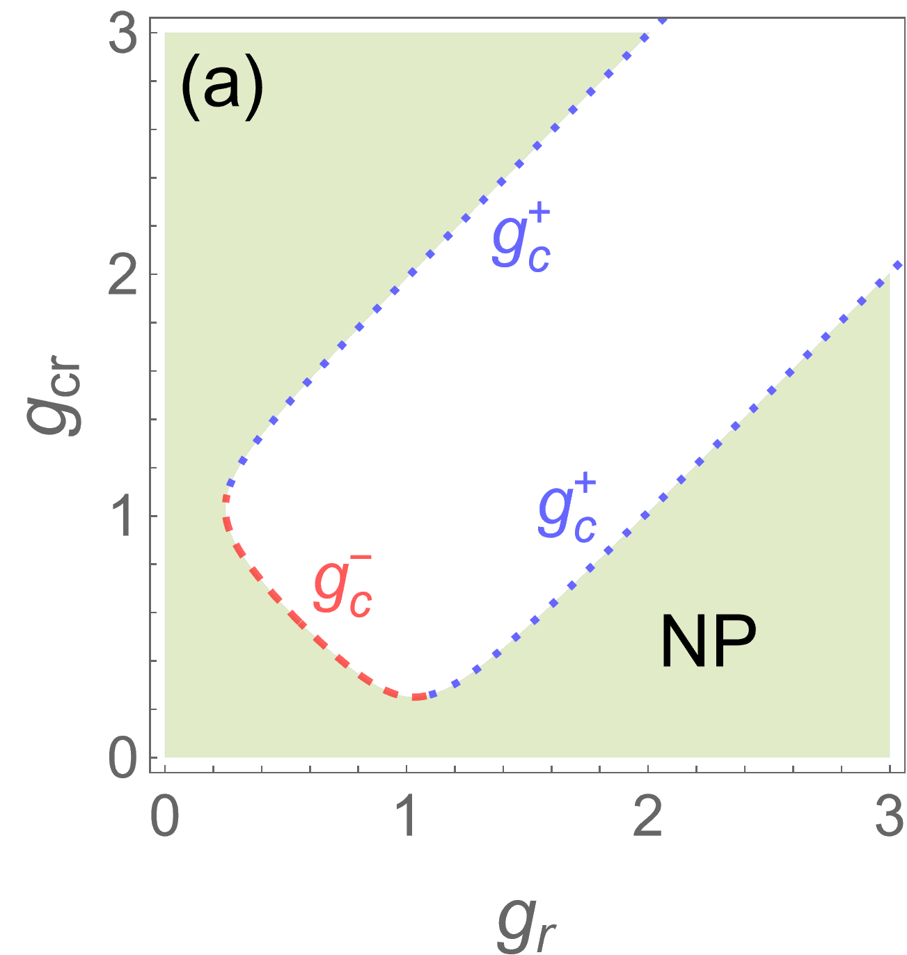
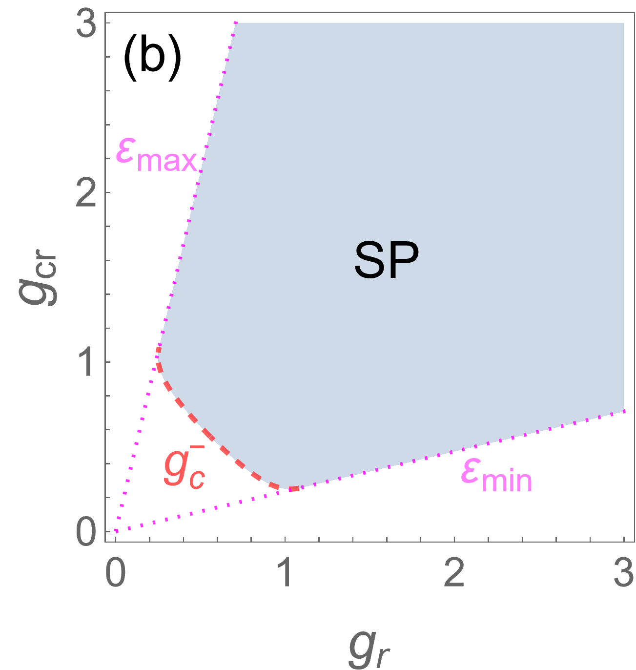
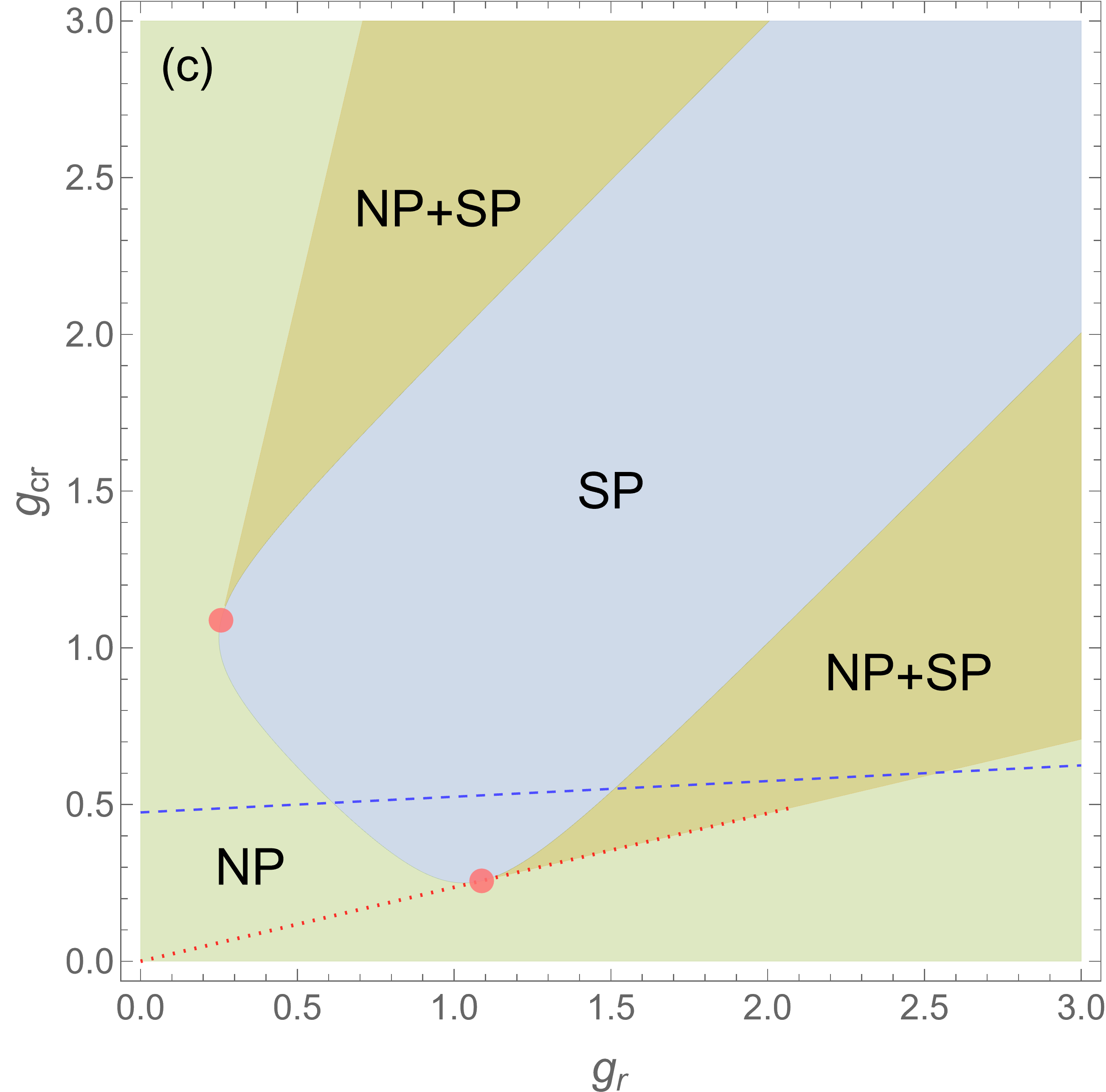
Figure 1: Phase diagram of the anisotropic open quantum Rabi model. (a) The stable region for the normal phase (NP) (shaded in green). The blue dotted and red dashed curves depict the critical coupling strength $g_{c}^{\pm}(\varepsilon,\bar{\kappa})$, respectively. (b) The stable region (shaded in blue) for the superradiant phase (SP). The red dashed curve $g_{c}^{-}(\varepsilon,\bar{\kappa})$ is the same one in (a). The magenta dotted line has the slope $\varepsilon_{\text{min (max)}}(\bar{\kappa})$. (c) The phase diagram. The overlap region between the NP in (a) and the SP in (b) is a bistable phase shaded in yellow. Two red dots, located at the intersection of three phases, represent the tricritical points. The dashed and dotted lines in (c) are used in later discussions. Here we set $\bar{\kappa}=0.5$.

The resulting rich phase diagram of the anisotropic open QRM is shown in Fig. 1(c). There are two notable features. First, a bistable phase emerges where the NP and SP phases coexist (shaded in yellow). In the symmetric case ($g_{cr}=g_{r}$), the system exhibits a transition from the NP to the SP when the coupling strength reaches the critical value ($g_{c}^{-}=\sqrt{1+\bar{\kappa}^{2}}/2$) and the NP remains unstable for any value of $g>g_{c}^{-}$ Hwang et al. (2018). However, by introducing an asymmetry in the coupling terms, the NP becomes stable again as one increases the coupling strengths even further beyond the critical value $g_{c}^{-}$, i.e. as $g>g_{c}^{+}(\varepsilon,\bar{\kappa})$, coexisting with the SP. Second, there is a tricritical point (red dot) located at the intersection of the three phases, where the phase boundary curve $g_{c}^{-}(\varepsilon,\bar{\kappa})$ (a boundary of a second-order phase transition) meets the phase boundary line $g_{cr}=g_{r}\varepsilon_{\text{min (max)}}$ (a boundary of a first-order phase transition).

In order to demonstrate the first-order and second-order DPT of the system, we plot in Fig. 2 the order parameter $\alpha$ as $g$ traverses the normal and superradiant phases along the blue dashed line in Fig. 1(c). When $g$ (namely $g_{r}$) goes a from the NP to the SP, the absolute value of $\alpha$ presents a second-order phase transition at the critical coupling strength $g_{c}^{-}\approx 0.61$. For convenience, we denote the value of $g$ at the phase boundary line $g_{cr}=g_{r}\varepsilon_{\text{min (max)}}$ as $g_{\varepsilon_{\text{min (max)}}}$. When crossing the phase boundary line at $g=g_{\varepsilon_{\text{min}}}\approx 2.55$, the order parameter $\alpha$ turns to zero abruptly, leading to a discontinuity of the order parameter and the first-order phase transition on the boundary line. We also note that there are two values of order parameter $|\alpha|$ in the range of the bistable phase between the the critical coupling strength $g_{c}^{+}\approx 1.51$ to the phase boundary line at $g_{\varepsilon_{\text{min}}}\approx 2.55$. Interestingly, due to the presence of the bistable phase, a hysteresis effect could be observed at the boundary between the normal and superradiant phases when $g$ crossing the bistable phase forward and backward. A similar hysteresis between the NP and SP has been experimentally observed using a driven BEC in a cavity system Ferri et al. (2021); Stitely et al. (2020).

In Figs. 1 and 2 we have chosen $\bar{\kappa}=0.5$. As one decreases $\bar{\kappa}$, the tricritical points approach the $g_{cr}$ and $g_{r}$ axes; therefore, the area of the NP shrinks. At the same time, the first-order phase transition boundary, given by $\varepsilon_{\textrm{min (max)}}(\bar{\kappa})$, becomes closer to $g_{c}$ and $g_{cr}$ axis, leading to the widening of the SP. As one increases $\bar{\kappa}$, the trend is reversed.

V Quantum fluctuations

Having established the mean-field phase diagram of the anisotropic open QRM, in this section we will provide a full quantum solution for the NP and the SP. First, we derive an effective master equation in the $\Omega/\omega_{0}\rightarrow\infty$ limit, characterized by a quadratic form involving the oscillator operator $a$. Utilizing this quadratic effective master equation, we study the cr itical scaling of quantum fluctuation and asymptotic decay rate near the phase boundaries and the tricitical point.

V.1 Normal phase

By performing the Schrieffer-Wolff (SW) transformation to the Hamiltonian (2) and projecting it to the spin-down subspace Hwang et al. (2015, 2018), we obtain an effective Hamiltonian for the NP, which reads

$$H_{\text{np}} =\omega_{0}a^{\dagger}a-\omega_{0}\left[g_{r}^{2}a^{\dagger}a+g_{cr}^{2}aa^{\dagger}+g_{r}g_{cr}(a^{\dagger 2}+a^{2})\right].$$ (26)

Note that the higher order terms whose coefficients become zero in the $\Omega/\omega_{0}\rightarrow\infty$ limit are neglected Hwang et al. (2015, 2018). Correspondingly, the effective master equation becomes

$$\dot{\rho}_{\text{np}}=-i[H_{\text{np}},\rho_{\text{np}}]+\kappa D[a]\rho_{\text{np}},$$ (27)

where the density matrix $\rho_{\text{np}}=\left\langle\textstyle{\downarrow}\right|\mathrm{e}^{-S}\rho\mathrm{e}^{S}\left|\textstyle{\downarrow}\right\rangle$ and the generator for the SW transformation is given by $S=\frac{\lambda_{r}}{\Omega}(a\sigma_{+}-a^{\dagger}\sigma_{-})-\frac{\lambda_{cr}}{\Omega}(a\sigma_{-}-a^{\dagger}\sigma_{+})$. Then, the equation of motion for the first moment of the oscillator operators, $\textbf{a}=(\left\langle\textstyle{a}\right\rangle,\left\langle\textstyle{a^{\dagger}}\right\rangle)^{\intercal}$, reads

$$\dot{\textbf{a}}=L_{\textrm{np}}\textbf{a}$$ (28)

where

(31)

The eigenvalue $l_{\textrm{np}}$ of $L_{\textrm{np}}/\omega_{0}$ reads

$$l_{\textrm{np}}^{\pm}=-\bar{\kappa}\pm\sqrt{2g^{2}\left(1+\varepsilon^{2}\right)-g^{4}\left(1-\varepsilon^{2}\right)^{2}-1}.$$ (32)

The NP is stable as long as the real part of the eigenvalues are negative. Since $\mathrm{Re}[l_{\textrm{np}}^{-}]$ is always negative, we only need to examine $l_{\textrm{np}}^{+}$. In Fig. 3(a), we plot the real part (green solid curve) and the imaginary part (red dotted curve) of $l_{\textrm{np}}^{+}$ for the case $g$ going along the blue dashed line in Fig. 1(c). For small $g$ far away from the critical point ($g\ll g_{c}^{-}(\varepsilon,\bar{\kappa})$), the square root term is pure imaginary. In this case, the dynamics of the system is underdamped and the decay rate is $\bar{\kappa}$. As $g$ approaches the the critical point, the dynamics becomes overdamped with a zero imaginary part. The effective decay rate in this overdamped region is called as an asymptotic decay rate (ADR), which tends to zero as $g$ approaches its critical values. This behavior is coincide with the closing of the Liouvillian gap near the critical point Kessler et al. (2012); Fitzpatrick et al. (2017); Hwang et al. (2018).

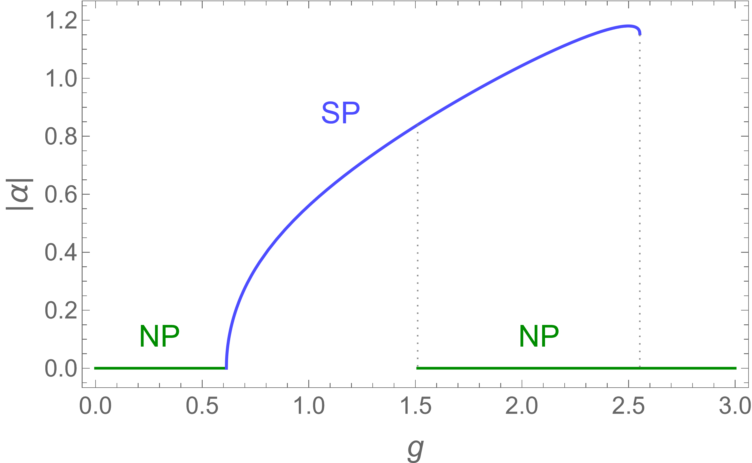
Figure 2: First- and second-order DPT and hysteresis due to bistability. The absolute value of the order parameter $\alpha$ as a function of $g$ (namely $g_{r}$) is depicted as one moves along the blue dashed line in Fig. 1(c), which is $g_{cr}=0.05(g_{r}-0.5)+0.5$.

For $g>g_{c}^{-}$, $\mathrm{Re}[l_{\textrm{np}}^{+}]$ becomes positive, so that the NP becomes unstable. We note however that the inner square root part of $l_{\textrm{np}}^{+}$ has an inverted parabolic shape with respect to $g^{2}$ when $\varepsilon\neq 1$.Therefore, upon further increasing $g$ with $\varepsilon\neq 1$, the real part of $l_{\textrm{np}}^{+}$ becomes negative again for $g>g_{c}^{+}(\varepsilon,\bar{\kappa})$ [See the light solid curve in Fig. 3(a)]. The recurrence of the NP therefore occurs due to the competition between the bare oscillator decay rate $\bar{\kappa}$ and the asymmetry $\varepsilon$ which results in a non-monotonic behavior of the ADR in the overdamped dynamics.

We also examine fluctuations of the oscillator excitation in the NP. The dynamics of the second moments $\textbf{s}=\left(\left\langle\textstyle{a^{\dagger}a}\right\rangle,\left\langle\textstyle{a^{2}}\right\rangle,\left\langle\textstyle{a^{\dagger 2}}\right\rangle\right)^{\intercal}$ of the oscillator is governed by

$$\dot{\textbf{s}}=M_{\textrm{np}}\textbf{s}+Y_{\textrm{np}},$$ (33)

where

(37)

and $Y_{\textrm{np}}=\omega_{0}\left(0,i2g_{r}g_{cr},-i2g_{r}g_{cr}\right)^{\intercal}$. The solution for the steady state is given by

$$\textbf{s}_{s}=-M_{\textrm{np}}^{-1}Y_{\textrm{np}}.$$ (38)

Explicitly, the excitation number of the oscillator for the steady state reads

$$\left\langle\textstyle{a^{\dagger}a}\right\rangle_{s}=\frac{2g^{4}\varepsilon^{2}}{g^{4}\left(1-\varepsilon^{2}\right)^{2}-2g^{2}\left(1+\varepsilon^{2}\right)+\bar{\kappa}^{2}+1}.$$ (39)

The number of excitations diverges at the boundary of the NP, and the divergence exhibits a power law, whose critical exponents are examined in the next section.

V.2 Superradiant phase

Let us now examine the quantum dynamics and fluctuations in the SP. Following the method in Ref. Hwang et al. (2018), we derive an effective master equation in the SP by applying a displacement unitary transformation $\mathcal{D}[\alpha]=\exp[\alpha a^{\dagger}-\alpha^{*}a]$ to the master equation, Eq. (1), followed by the SW transformation. See details in Appendix  C. The effective master equation for the SP becomes

$$\dot{\rho}_{\text{sp}}=-i[H_{q},\rho_{\text{sp}}]+\kappa D[a]\rho_{\text{sp}},$$ (40)

where the quadratic effective Hamiltonian $H_{q}$ reads

$$H_{q}=Pa^{\dagger}a+Qaa+Q^{*}a^{\dagger}a^{\dagger}.$$ (41)

The expressions for the coefficients $P$ and $Q$ are quite involved and they are given in Eqs. (73) and (74) in Appendix  C.

The dynamics of the mean value of the oscillator operator is determined by $\dot{\textbf{a}}=L_{\textrm{sp}}\textbf{a}$ with

$$L_{\textrm{sp}}=\left(\begin{array}[]{cc}-iP-\kappa&-i2Q^{*}\\ i2Q&iP-\kappa\end{array}\right).$$ (44)

The eigenvalues $l_{\textrm{sp}}$ of $L_{\textrm{sp}}/\omega_{0}$ are given by

$$l^{\pm}_{\textrm{sp}}=-\bar{\kappa}\pm\frac{1}{\omega_{0}}\sqrt{4|Q|^{2}-P^{2}}.$$ (45)

The stability condition of the SP, $\mathrm{Re}[l_{\textrm{sp}}^{\pm}]<0$, agrees well with the stable area for the SP as shown in Fig. 1(b). The real part (blue dashed curve) and imaginary part (orange dash-dotted curve) of $l_{\textrm{sp}}^{+}$ and are shown in Fig. 3(a), where $g$ goes along the blue dashed line in Fig. 1(c). Similar to the NP, the real part of $l_{\textrm{sp}}^{+}$ approaches zero at phase boundaries of the SP, leading to a vanishing ADR. In Fig. 3(a), we observe a range of $g$, $1.51\lesssim g\lesssim 2.55$, where the real part of both $l_{\textrm{sp}}^{+}$ and $l_{\textrm{np}}^{+}$ are negative, which indicates the emergence of the bistable phase.

By solving the equation of motion of the second moments, we find that the excitation number of the oscillator in the SP is given by

$$\left\langle\textstyle{a^{\dagger}a}\right\rangle_{s}=\frac{2|Q|^{2}}{P^{2}-4|Q|^{2}+\kappa^{2}}.$$ (46)

As shown in Fig. 4(a), the excitation number diverges in the SP at the phase boundaries.

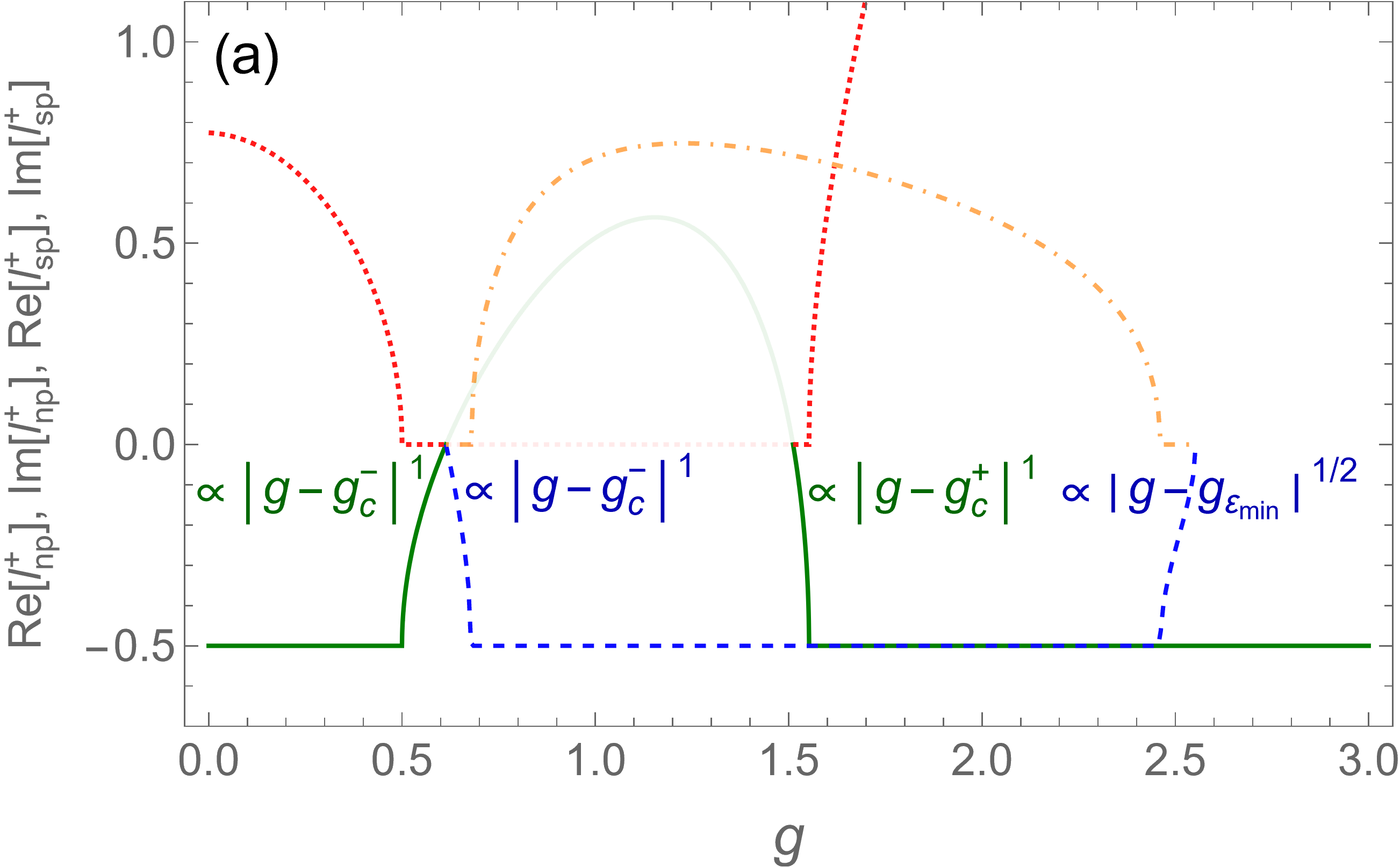
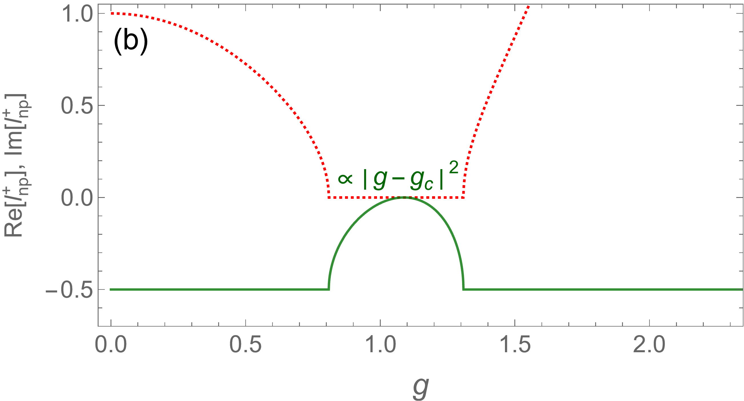
Figure 3: Asymptotic decay rate (ADR) for the NP and the SP. (a) The eigenvalues of dynamical matrices $l^{+}_{\textrm{np (sp)}}$ as a function of $g$ are presented as one moves along the blue dashed line in Fig. 1(c). The real (imaginary) part of $l^{+}_{\textrm{np}}$ and $l^{+}_{\textrm{sp}}$ is given by green solid (red dotted) curve and blue dashed (orange dash-dotted) curve, respectively. (b) The real and imaginary parts of $l^{+}_{\textrm{np}}$ as one moves along the red dotted line in Fig. 1(c), which is the phase boundary line $g_{cr}=g_{r}\varepsilon_{\text{min}}$. The scaling of ADR near the critical coupling strengths $g_{c}^{\pm}$ and $g_{\varepsilon_{\text{min}}}$ is presented in each panel. Here $\bar{\kappa}=0.5$.

VI Universality of the tricritical point

Using the quantum solutions derived in the previous section, we now examine the universality for the DPTs in the anisotropic open QRM. The closing of the Liouvillian gap, thus the vanishing ADR, and the diverging oscillator excitation number are the characteristic features of a second-order DPT driven by a Markovian bath Torre et al. (2013); Hwang et al. (2018). These features can be clearly seen in Figs. 3(a) and 4(a).

First, let us focus on the critical curve $g_{c}^{-}(\varepsilon_{\text{min}}<\varepsilon<\varepsilon_{\text{max}},\bar{\kappa})$ at which a second-order phase transition occurs. On both sides of the critical curve, the ADR vanishes as

$$\kappa_{\textrm{ADR}}=\mathrm{Re}[l_{\textrm{np (sp)}}^{+}]\propto|g-g_{c}^{-}(\varepsilon,\bar{\kappa})|^{\nu_{\textrm{ADR}}}.$$ (47)

with $\nu_{\textrm{ADR}}=1$ and the oscillator population diverges as

$$\left\langle\textstyle{a^{\dagger}a}\right\rangle_{s}\propto|g-g_{c}^{-}(\varepsilon,\bar{\kappa})|^{-\nu_{x}}.$$ (48)

with the exponent $\nu_{x}=1$. Therefore, the second-order DPT along the critical curve $g_{c}^{-}$ belongs to the same universality class as the symmetric open QRM Hwang et al. (2018) and open Dicke model Torre et al. (2013).

Second, we have two additional critical lines where a first-order phase transition occurs due to the bistability. In equilibrium, correlation functions and fluctuations typically do not diverge at the first-order phase transition Nishimori and Ortiz (2010). In stark contrast, in our nonequilibrium model, the number of oscillator excitations (a fluctuation of the order parameter) diverges with a power-law at the first-order phase transition. The exponents at the first-order phase boundary of the NP, $g_{c}^{+}(\varepsilon,\kappa)$, are the same with those of second-order phase transition, namely, $\nu_{\textrm{ADR}}=\nu_{x}=1$. At the first-order boundary of the SP, on the other hand, we find a new set of exponents $\nu_{\textrm{ADR}}=\nu_{x}=1/2$ [See Figs. 3(a) and 4(a)]. Our finding shows that the nonequilibrium first-order DPTs driven by a Markovian bath could show drastically different critical properties from its equilibrium counterpart Nishimori and Ortiz (2010). We note that the denominator of the excitation number in Eq. (39) has the same roots [i.e. $g_{c}^{\pm}(\varepsilon,\bar{\kappa})$] as the eigenvalue of $l_{\text{np}}^{+}$ in Eq. (32). The same holds for the SP case, as seen in Eqs. (46) and (45). Therefore, the ADR vanishes at the critical coupling strengths $g_{c}^{\pm}$ and $g_{\varepsilon_{\text{min}}}$ with the same critical exponent that governs the divergence of excitation number [See Figs. 3(a) and 4(a)].

The critical exponents of the tricritical point are typically different from those of second-order phase transition Nishimori and Ortiz (2010); therefore, it is interesting to examine the criticality of the tricritical point $g_{c}^{-}(\varepsilon_{\text{min (max)}},\bar{\kappa})$. We find that the critical exponents depend on the angle at which one crosses the critical point. The novel critical behaviors along the line $g_{cr}=g_{r}\varepsilon_{\text{min}}$ are presented in Figs. 3(b) and 4(b), which shows that the critical exponents are given as $\nu_{\textrm{ADR}}=\nu_{x}=2$. We note that $g_{cr}=g_{r}\varepsilon_{\min}$ is actually the tangent line of the NP boundary at the tricritical point. Along this line, both sides of the tricritical point are the NP and there is no phase transition. In fact, if one moves along any line that is tangent to the phase boundary of the NP, we find the identical critical behaviors shown in Figs. 3(b) and 4(b). To understand this set of higher critical exponents, one can see the real part of $\l_{\text{np}}^{+}$ shown in Fig. 3(b). Near the critical value $g_{c}\approx 1.1$, the top of the parabolic-like curve ($\mathrm{Re}[l_{\text{np}}^{+}]$) touches $0$, and therefore presenting the critical exponent $\nu_{\textrm{ADR}}=2$. But if $\mathrm{Re}[l_{\text{np}}^{+}]$ gets greater than zero, indicating that $g$ goes across the critical point $g_{c}$ and the system goes though a phase transition, the critical exponent will turn to $\nu_{\text{ADR}}=1$ as the case shown in Fig. 3(a). This showcases the peculiarity of the tangent line along the convex boundary of the NP, which leads to a set of higher scaling exponents $\nu_{\text{ADR}}=\nu_{x}=2$. Furthermore, we verify that this property is also applicable for the generalized open Dicke model Soriente et al. (2018). Our analysis demonstrates that the non-monotonic phase boundary due to the competition between the dissipation and the coherent interaction gives rise to various ways of crossing the critical points with different critical exponents. It would be interesting to investigate whether these novel critical scalings could be used to improve the critical sensing schemes based on the open QRM Ilias et al. (2022, 2023).

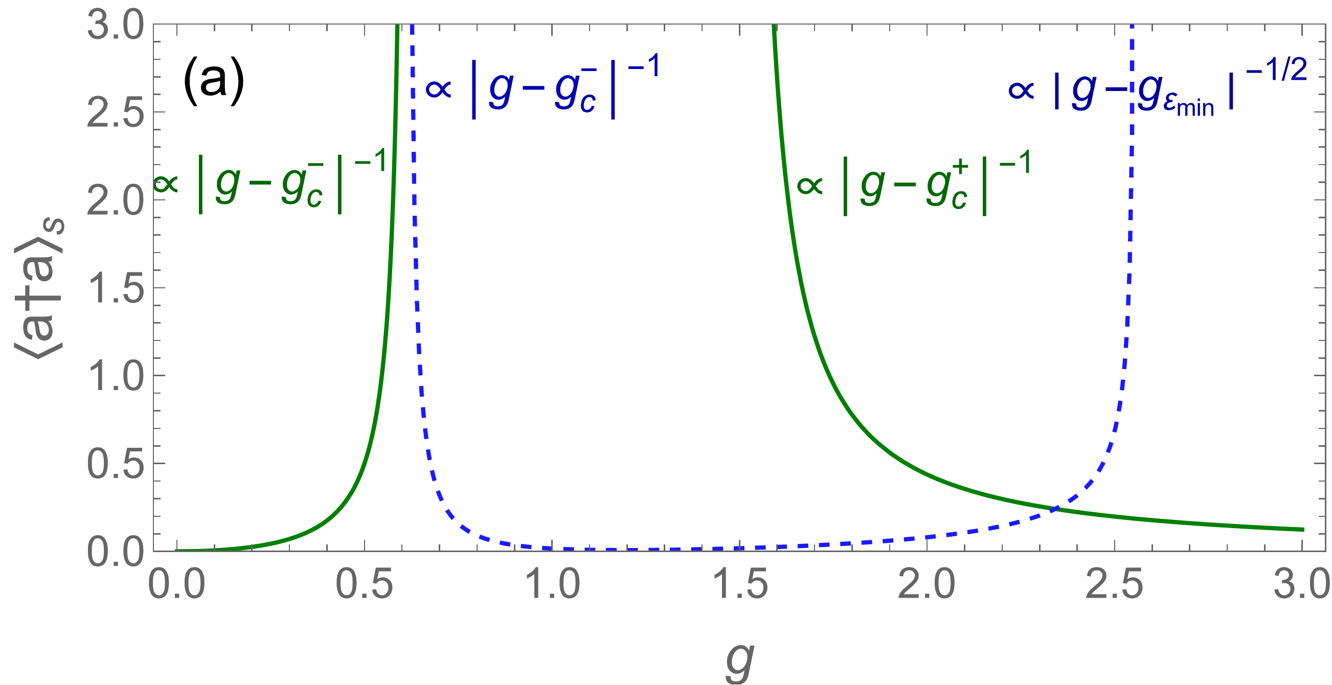
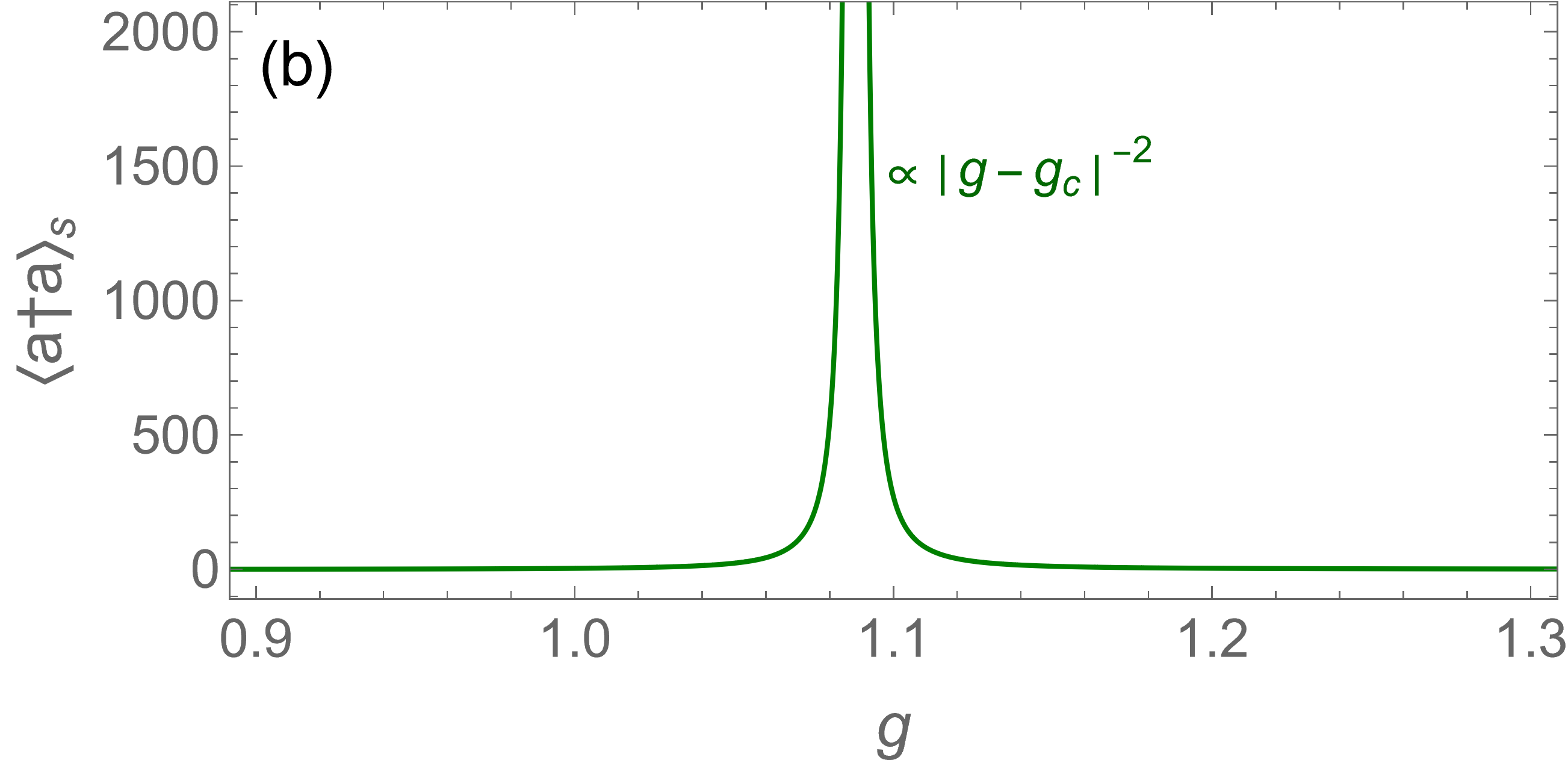
Figure 4: Critical scaling of the oscillator population. The oscillator population for the NP (green solid) and the SP (blue dashed) as a function of $g$ is plotted as one moves (a) along the blue dashed line and (b) along the red dotted line in Fig. 1(c). The latter represents the critical behavior across the tricrical point. The scaling exponent near the critical coupling strength is presented in each panel. Here, $\bar{\kappa}=0.5$.

VII Implementation

Ref. Hwang et al. (2018) proposed to use a trapped-ion setup involving two ions to implement the open QRM. Here, we briefly review the proposal and discuss how the same setup could be used to realize the anisotropic open QRM.

Consider a mixed species ion pair, ${}^{9}{\rm Be^{+}-^{24}}{\rm Mg}^{+}$ Lin et al. (2013); Tan et al. (2015), in a linear Paul trap. The common center-of-mass mode can be used as the oscillator realizing the open QRM, while all other vibration modes are significantly detuned. The hyperfine states of the ${}^{9}{\rm Be^{+}}$ ion, specifically $\left|\textstyle{F=2,m_{F}=0}\right\rangle$ and $\left|\textstyle{F=1,m_{F}=1}\right\rangle$, form a qubit that can be coupled to the motional mode through coherent stimulated Raman transitions Monroe et al. (1995). By applying two lasers to the ${}^{9}{\rm Be^{+}}$ ion, with detunings $\delta_{1}$ and $\delta_{2}$, we drive the red- and blue-sideband transitions. The intensity of the two lasers can be controlled independently to realize different Rabi frequencies $\Omega_{1}^{d}$ and $\Omega_{2}^{d}$. In the interaction picture with respect to the bare qubit and oscillator dynamics, followed by a rotating wave approximation, the interaction Hamiltonian between the oscillator and the qubit in the Lamb-Dicke limit can be expressed as $H_{I}=-\eta_{\rm LD}\Omega_{1}^{d}/2(\sigma_{+}a^{\dagger}\mathrm{e}^{i\delta_{1}t}+\mathrm{H.c.})-\eta_{\rm LD}\Omega_{2}^{d}/2(\sigma_{+}a\mathrm{e}^{i\delta_{2}t}+\text{H.c.})$, where $\eta_{\rm LD}$ represents the Lamb-Dicke parameter. Moving to the rotating frame of $H_{\text{rot}}=\sigma_{z}(\delta_{1}+\delta_{2})/4+a^{\dagger}a(\delta_{1}-\delta_{2})/2$, the interaction Hamiltonian $H_{I}$ turns into the form of our Rabi Hamiltonian (2). In this frame, the parameters of the Rabi Hamiltonian are given by $\omega_{0}=(\delta_{1}-\delta_{2})/2$, $\Omega=(\delta_{1}+\delta_{2})/2$, $\lambda_{cr}=\eta_{\rm LD}\Omega_{1}^{d}/2$, and $\lambda_{r}=\eta_{\rm LD}\Omega_{2}^{d}/2$ Pedernales et al. (2015); Puebla et al. (2017). Therefore, simply by controlling the relative intensities of the Raman lasers driving blue and red side band transitions, one could realize the anisotropic Rabi model. The dissipation to the oscillator can be achieved by using the sympathetic cooling Lin et al. (2013); Tan et al. (2015) of the center-of-mass mode with the second ion, ${}^{24}{\rm Mg}^{+}$. Previous experimental studies have successfully demonstrated the sympathetic cooling for the in-phase mode using ${}^{24}{\rm Mg}^{+}$ ions Lin et al. (2013); Tan et al. (2015). Moreover, it has been experimentally demonstrated that coherent bosonic states with a large number of excitations can be generated for the motional modes in ion-traps using sideband transitions and dissipation Kienzler et al. (2015, 2017); Behrle et al. (2023).

VIII Conclusion

In conclusion, we have investigated a rich steady-state phase diagram of the anisotropic open QRM. It features a number of interesting critical phenomena resulting from the competion between the anisotropic interaction and the dissipation. First, there are two critical ratios, $\varepsilon_{\textrm{min}}$ and $\varepsilon_{\textrm{max}}$, between the interaction strengths of the counterrotating terms and the rotating terms, beyond and below which no DPT occurs. In such cases, the Markovian bath brings the system to a trivial steady state, regardless of the strength of the coherent interaction. Second, in between these critical ratios, a second-order DPT occurs where the NP becomes unstable and the SP with a broken symmetry emerges. Strikingly, upon increasing further the coherent interaction strength beyond the second-order DPT, the NP becomes stable again, leading a bistable phase of the NP and the SP. The boundaries of the bistable phase are characterized by a first-order DPT. Moreover, a tricritical point appears where the critical lines for the second-order and the first-order DPTs meet. Third, the tricritical point features a novel set of critical exponents. It is an interesting question to see whether the novel scaling behavior of the tricritical point could be harnessed for the critical quantum sensing protocol based on the open QRM  Ilias et al. (2022, 2023). Our work demonstrates that interesting nonequilibrium critical phenomena such as multicriticality and bistability can be explored in a finite-component systems with a controlled coherent interaction and damping, realized by two trapped ions.

Appendix A Stability Analysis

Here, we provide a stability analysis for the mean-field solutions. To this end, we consider small deviations from the mean-field solutions given in Eqs. (3-5): $\left\langle\textstyle{a}\right\rangle\mapsto\bar{\alpha}+\delta\bar{\alpha}$, $\left\langle\textstyle{\sigma_{+}}\right\rangle\mapsto s_{+}+\delta s_{+}$, and $\left\langle\textstyle{\sigma_{z}}\right\rangle\mapsto s_{z}+\delta s_{z}$. Here we have introduced mean-field amplitude $\bar{\alpha}$ for the operator $a$: $\bar{\alpha}\equiv\left\langle\textstyle{a}\right\rangle\equiv\bar{x}+i\bar{y}$ and note that $\sqrt{\frac{\omega_{0}}{\Omega}}\bar{\alpha}=\alpha\equiv x+iy$. Considering only the first-order terms for the fluctuation, we obtain that

$$\dfrac{d}{dt}\delta\bar{\alpha}=-i(\omega_{0}-i\kappa)\delta\bar{\alpha}+i(\lambda_{r}\delta s_{-}+\lambda_{cr}\delta s_{+}),$$ (49)

(50)

(51)

By introducing $\delta\bar{\alpha}\equiv\delta\bar{x}+i\delta\bar{y}$ and $\delta s_{+}\equiv(\delta s_{x}+i\delta s_{y})/2$, and using the condition for the spin conservation $s_{x}^{2}+s_{y}^{2}+s_{z}^{2}=1$, the dynamical equation becomes

$$\dfrac{d}{dt}\begin{pmatrix}\delta\bar{x}\\ \delta\bar{y}\\ \delta s_{x}\\ \delta s_{y}\\ \end{pmatrix}=\begin{pmatrix}-\kappa&\omega_{0}&0&\lambda(1-\varepsilon)/2\\ -\omega_{0}&-\kappa&\lambda(1+\varepsilon)/2&0\\ 0&2\lambda(1-\varepsilon)s_{z}&-2\lambda(1-\varepsilon)\bar{y}\frac{s_{x}}{s_{z}}&-\left(2\lambda(1-\varepsilon)\bar{y}\frac{s_{y}}{s_{z}}+\Omega\right)\\ 2\lambda(1+\varepsilon)s_{z}&0&-\left(2\lambda(1+\varepsilon)\bar{x}\frac{s_{x}}{s_{z}}-\Omega\right)&-2\lambda(1+\varepsilon)\bar{x}\frac{s_{y}}{s_{z}}\end{pmatrix}\begin{pmatrix}\delta\bar{x}\\ \delta\bar{y}\\ \delta s_{x}\\ \delta s_{y}\\ \end{pmatrix}.$$ (52)

The eigenvalues $\mu$ of the above matrix determines the stability of the mean-value solutions. Considering the limit of $\Omega/\omega_{0}\rightarrow\infty$, we find that the characteristic equation up to the leading order term of $\Omega/\omega_{0}$, which reads $A{\omega_{0}}^{2}+2\bar{\kappa}B\omega_{0}\mu+B\mu^{2}=0$ where

$$A =1+\bar{\kappa}^{2}+4g^{2}(1+\bar{\kappa}^{2})[(-1+\varepsilon)^{2}y^{2}+(1+\varepsilon)^{2}x^{2}]$$

$$\quad+2g^{2}(1+\varepsilon^{2})s_{z}+g^{4}(-1+\varepsilon^{2})^{2}[s_{z}^{2}+4s_{z}(x^{2}+y^{2})],$$ (53)

$$B =1+4g^{2}\left[(-1+\varepsilon)^{2}y^{2}+(1+\varepsilon)^{2}x^{2}\right].$$ (54)

Note that we have used the expressions of $s_{x}$ and $s_{y}$ given in Eq. (21) to rewrite the coefficients given above. Finally, we obtain the eigenvalue

$$\mu/\omega_{0}=-\bar{\kappa}\pm\sqrt{\bar{\kappa}^{2}-A/B}.$$ (55)

The stability condition $\text{Re}(\mu)<0$ reduces to $A>0$, because $B$ is always positive.

Appendix B Stability of the Nontrivial Solution with $s_{z}^{+}$

Here, we check the stability of the nontrivial solution $s_{z}=s_{z}^{+}\equiv-[(1+\varepsilon^{2})+\sqrt{4\varepsilon^{2}-\bar{\kappa}^{2}(1-\varepsilon^{2})^{2}}]/(1-\varepsilon^{2})^{2}g^{2}$ for Eq. (17). By substituting $s_{z}^{+}$, $x$ [Eq. (19)], and $y$ [Eq. (20)] into the coefficient $A$ given in Eq. (A), we find that the stability condition $A>0$ is equivalent to

$$g<\sqrt{\frac{(1+\varepsilon^{2})+\sqrt{4\varepsilon^{2}-\bar{\kappa}^{2}(1-\varepsilon^{2})^{2}}}{(1-\varepsilon^{2})^{2}}}.$$ (56)

We notice that the right hand side of the inequality is the same as the value of $g_{c}^{+}(\varepsilon,\bar{\kappa})$ given in Eq. (24). The critical coupling strength $g_{c}^{+}(\varepsilon,\bar{\kappa})$ is shown by the blue dotted curves in Fig. A1. The solution for the $s_{z}$ is meaningful only when $-1<s_{z}^{+}<1$. We plot the region $-1<s_{z}^{+}<1$ in gray in Fig. A1. In this region, the condition (56) is not satisfied, therefore, the physical solution of the $s_{z}^{+}$ is unstable.

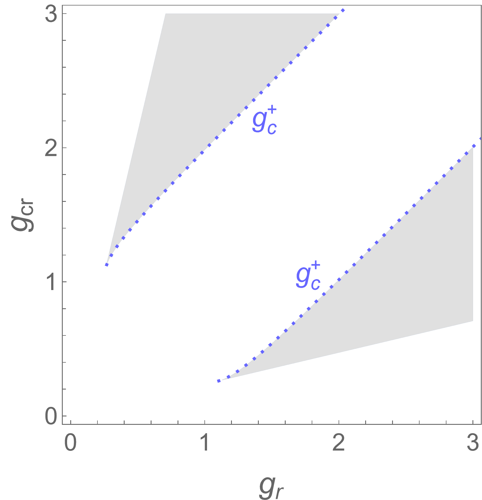
Figure A1: Physical region for the nontrivial solution with $s_{z}^{+}$. The blue dotted curves represent the critical coupling strength $g_{c}^{+}(\varepsilon,\bar{\kappa})$. The gray area shows the physical allowed region with $-1<s_{z}^{+}<1$. Here we set $\bar{\kappa}=0.5$.

Appendix C Effective Hamiltonian for the Superradiant Phase

In this section, we derive an effective Hamiltonian for the SP. First, we apply a displacement unitary transformation to original master equation (1), with the displacement operator $\mathcal{D}[\alpha_{s}]=\exp[\alpha_{s}a^{\dagger}-\alpha_{s}^{*}a]$. Setting that $\alpha_{s}$ equals the mean-field amplitude of the oscillator in the superradiant state, namely $\alpha_{s}=\left\langle\textstyle{a}\right\rangle\equiv\bar{\alpha}$, the master equation becomes

$$\dot{\bar{\rho}}=-i[\bar{H}(\bar{\alpha}),\bar{\rho}]+\kappa(2a\bar{\rho}a^{\dagger}-a^{\dagger}a\bar{\rho}-\bar{\rho}a^{\dagger}a),$$ (57)

where $\bar{\rho}\equiv\mathcal{D}^{\dagger}[\alpha_{s}]\rho\mathcal{D}[\alpha_{s}]$ and the effective unitary Hamiltonian $\bar{H}(\bar{\alpha})$ is given by

$$\bar{H}(\bar{\alpha}) =\mathcal{D}^{\dagger}[\bar{\alpha}]H\mathcal{D}[\bar{\alpha}]+i\kappa(\bar{\alpha}^{*}a-\bar{\alpha}a^{\dagger})$$

$$=H_{s}-V+H_{f},$$ (58)

with the terms

$$H_{s} =\frac{\Omega}{2}\sigma_{z}-\sigma_{+}(\lambda_{r}\bar{\alpha}+\lambda_{cr}\bar{\alpha}^{*})-\sigma_{-}(\lambda_{r}\bar{\alpha}^{*}+\lambda_{cr}\bar{\alpha}),$$ (59)

$$V =\lambda_{r}(a\sigma_{+}+a^{\dagger}\sigma_{-})+\lambda_{cr}(a\sigma_{-}+a^{\dagger}\sigma_{+}),$$ (60)

$$H_{f} =\omega_{0}\left(a^{\dagger}a+a^{\dagger}\bar{\alpha}(1-i\bar{\kappa})+a\bar{\alpha}^{*}(1+i\bar{\kappa})+|\bar{\alpha}|^{2}\right).$$ (61)

We note that the spin part of the $H_{s}$ term can be diagonalized in terms of $U^{\dagger}H_{s}U=\frac{\Omega}{2}\sqrt{\xi}\sigma_{z}$ by the unitary operator

$$U=\frac{1}{\sqrt{2}\sqrt{\xi+\sqrt{\xi}}}\begin{pmatrix}1+\sqrt{\xi}&2(g_{r}\alpha+g_{cr}\alpha^{*})\\ -2(g_{r}\alpha^{*}+g_{cr}\alpha)&1+\sqrt{\xi}\end{pmatrix},$$ (62)

where we have used the abbreviation $\xi\equiv 1+4|g_{r}\alpha^{*}+g_{cr}\alpha|^{2}=1/s_{z}^{2}$. Correspondingly, the $V$ term becomes

$$U^{\dagger}VU =(a\sigma_{+}u^{*}+a^{\dagger}\sigma_{-}u)+(a\sigma_{-}v+a^{\dagger}\sigma_{+}v^{*})$$

$$\quad-(aw+a^{\dagger}w^{*})\sigma_{z},$$ (63)

where we have defined $u\equiv\sqrt{\Omega\omega_{0}}\bar{u}$, $v\equiv\sqrt{\Omega\omega_{0}}\bar{v}$ and $w\equiv\sqrt{\Omega\omega_{0}}\bar{w}$, and $\bar{u}$, $\bar{v}$ and $\bar{w}$ are given as follows

$$\bar{u} =\frac{1}{2}\left(g_{r}\left(1+\frac{1}{\sqrt{\xi}}\right)-g_{cr}\frac{(g_{r}\alpha^{*}+g_{cr}\alpha)^{2}}{\xi+\sqrt{\xi}}\right),$$ (64)

$$\bar{v} =\frac{1}{2}\left(g_{cr}\left(1+\frac{1}{\sqrt{\xi}}\right)-g_{r}\frac{(g_{r}\alpha^{*}+g_{cr}\alpha)^{2}}{\xi+\sqrt{\xi}}\right),$$ (65)

$$\bar{w} =\frac{1}{\sqrt{\xi}}[g_{r}(g_{r}\alpha^{*}+g_{cr}\alpha)+g_{cr}(g_{r}\alpha+g_{cr}\alpha^{*})].$$ (66)

Now, the effective unitary Hamiltonian $\bar{H}(\bar{\alpha})$ can be separated into diagonal and off-diagonal parts in the new spin basis

$$\bar{H}(\bar{\alpha}) =H_{d}-H_{od},$$ (67)

with

$$H_{d} =\omega_{0}a^{\dagger}a+\frac{\Omega}{2}\sqrt{\xi}\sigma_{z}+\omega_{0}|\bar{\alpha}|^{2}+H_{l},$$ (68)

$$H_{od} =(a\sigma_{+}u^{*}+a^{\dagger}\sigma_{-}u)+(a\sigma_{-}v+a^{\dagger}\sigma_{+}v^{*}).$$ (69)

In the diagonal part, there is a term $H_{l}$ which is linear in $a$ ($a^{\dagger}$): $H_{l}=a^{\dagger}[\omega_{0}\bar{\alpha}(1-i\bar{\kappa})+w^{*}\sigma_{z}]+a[\omega_{0}\bar{\alpha}^{*}(1+i\bar{\kappa})+w\sigma_{z}]$. We neglect this term in the following SW transformation, because it simply vanishes upon projection to the spin-down subspace.

Then, we perform the SW transformation to the Hamiltonian (67) with the generator

$$S^{\prime}\simeq\frac{1}{\Omega\sqrt{\xi}}(u^{*}a\sigma_{+}-ua^{\dagger}\sigma_{-})+\frac{1}{\Omega\sqrt{\xi}}(v^{*}a^{\dagger}\sigma_{+}-va\sigma_{-}),$$ (70)

where the approximation $1/(\Omega\sqrt{\xi}\pm\omega_{0})\simeq 1/\Omega\sqrt{\xi}$ is taken. By projecting it to the spin-down subspace, we finally obtain an diagonalized effective Hamiltonian for the SP,

$$\bar{H}_{\textrm{sp}}=H_{q}+E_{\text{sp}},$$ (71)

where $E_{\text{sp}}=\omega_{0}|\bar{\alpha}|^{2}-\frac{\Omega}{2|s_{z}|}-\omega_{0}|s_{z}||\bar{v}|^{2}$ is the ground energy, and $H_{q}$ has a quadratic from:

$$H_{q}=Pa^{\dagger}a+Qaa+Q^{*}a^{\dagger}a^{\dagger},$$ (72)

with the coefficients $P$ and $Q$ given as

$$P= \omega_{0}\left[1-|s_{z}|(|\bar{u}|^{2}+|\bar{v}|^{2})\right],$$ (73)

$$Q= -\omega_{0}|s_{z}|\bar{u}^{*}\bar{v}.$$ (74)

In addition, the expressions for $\bar{u}$ and $\bar{v}$ given in Eqs. (64) and (65) can be further simplified by substituting the explicit expressions of $x$ and $y$ in Eqs. (19) and (20):

$$\bar{u} =\frac{g}{2}\left[1+|s_{z}|-\frac{1}{2}(1-|s_{z}|)\sqrt{4\varepsilon^{2}-\bar{\kappa}^{2}(1-\varepsilon^{2})^{2}}\right]$$

$$\quad+i\frac{g}{4}(1-|s_{z}|)|1-\varepsilon^{2}|\bar{\kappa},$$ (75)

$$\bar{v} =\frac{g}{2}\left[\varepsilon(1+|s_{z}|)-\frac{1}{2\varepsilon}(1-|s_{z}|)\sqrt{4\varepsilon^{2}-\bar{\kappa}^{2}(1-\varepsilon^{2})^{2}}\right]$$

$$\quad+i\frac{g}{4\varepsilon}(1-|s_{z}|)|1-\varepsilon^{2}|\bar{\kappa}.$$ (76)

References

- Breuer and Petruccione (2002) H.-P. Breuer and F. Petruccione, The theory of open quantum systems (Oxford University Press, 2002).
- Müller et al. (2012) M. Müller, S. Diehl, G. Pupillo, and P. Zoller, Advances in Atomic, Molecular, and Optical Physics 61, 1 (2012).
- Rotter and Bird (2015) I. Rotter and J. P. Bird, Reports on Progress in Physics 78, 114001 (2015).
- Daley (2014) A. J. Daley, Advances in Physics 63, 77 (2014).
- Sieberer et al. (2016) L. M. Sieberer, M. Buchhold, and S. Diehl, Reports on Progress in Physics 79, 096001 (2016).
- Ashida et al. (2020) Y. Ashida, Z. Gong, and M. Ueda, Advances in Physics 69, 249 (2020).
- Rossini and Vicari (2021) D. Rossini and E. Vicari, Physics Reports 936, 1 (2021), coherent and dissipative dynamics at quantum phase transitions.
- Raghunandan et al. (2018) M. Raghunandan, J. Wrachtrup, and H. Weimer, Phys. Rev. Lett. 120, 150501 (2018).
- Minganti et al. (2021) F. Minganti, I. I. Arkhipov, A. Miranowicz, and F. Nori, New Journal of Physics 23, 122001 (2021).
- Casteels et al. (2017) W. Casteels, R. Fazio, and C. Ciuti, Phys. Rev. A 95, 012128 (2017).
- Krimer and Pletyukhov (2019) D. O. Krimer and M. Pletyukhov, Phys. Rev. Lett. 123, 110604 (2019).
- Minganti et al. (2018) F. Minganti, A. Biella, N. Bartolo, and C. Ciuti, Phys. Rev. A 98, 042118 (2018).
- Kessler et al. (2012) E. M. Kessler, G. Giedke, A. Imamoglu, S. F. Yelin, M. D. Lukin, and J. I. Cirac, Phys. Rev. A 86, 012116 (2012).
- Rodriguez et al. (2017) S. R. K. Rodriguez, W. Casteels, F. Storme, N. Carlon Zambon, I. Sagnes, L. Le Gratiet, E. Galopin, A. Lemaître, A. Amo, C. Ciuti, and J. Bloch, Phys. Rev. Lett. 118, 247402 (2017).
- Fink et al. (2018) T. Fink, A. Schade, S. Höfling, C. Schneider, and A. Imamoglu, Nature Physics 14, 365 (2018).
- Li et al. (2022) Z. Li, F. Claude, T. Boulier, E. Giacobino, Q. Glorieux, A. Bramati, and C. Ciuti, Phys. Rev. Lett. 128, 093601 (2022).
- Tomita et al. (2017) T. Tomita, S. Nakajima, I. Danshita, Y. Takasu, and Y. Takahashi, Science Advances 3, e1701513 (2017).
- Benary et al. (2022) J. Benary, C. Baals, E. Bernhart, J. Jiang, M. Röhrle, and H. Ott, New Journal of Physics 24, 103034 (2022).
- Sheremet et al. (2023) A. S. Sheremet, M. I. Petrov, I. V. Iorsh, A. V. Poshakinskiy, and A. N. Poddubny, Rev. Mod. Phys. 95, 015002 (2023).
- Fitzpatrick et al. (2017) M. Fitzpatrick, N. M. Sundaresan, A. C. Y. Li, J. Koch, and A. A. Houck, Phys. Rev. X 7, 011016 (2017).
- Fink et al. (2017) J. M. Fink, A. Dombi, A. Vukics, A. Wallraff, and P. Domokos, Phys. Rev. X 7, 011012 (2017).
- Baumann et al. (2010) K. Baumann, C. Guerlin, F. Brennecke, and T. Esslinger, Nature 464, 1301 (2010).
- Baumann et al. (2011) K. Baumann, R. Mottl, F. Brennecke, and T. Esslinger, Phys. Rev. Lett. 107, 140402 (2011).
- Brennecke et al. (2013) F. Brennecke, R. Mottl, K. Baumann, R. Landig, T. Donner, and T. Esslinger, PNAS 110, 11763 (2013).
- Klinder et al. (2015) J. Klinder, H. Keßler, M. Wolke, L. Mathey, and A. Hemmerich, PNAS 112, 3290 (2015).
- Baden et al. (2014) M. P. Baden, K. J. Arnold, A. L. Grimsmo, S. Parkins, and M. D. Barrett, Phys. Rev. Lett. 113, 020408 (2014).
- Hamner et al. (2014) C. Hamner, C. Qu, Y. Zhang, J. Chang, M. Gong, C. Zhang, and P. Engels, Nature communications 5, 4023 (2014).
- Kollár et al. (2017) A. J. Kollár, A. T. Papageorge, V. D. Vaidya, Y. Guo, J. Keeling, and B. L. Lev, Nature communications 8, 14386 (2017).
- Kroeze et al. (2018) R. M. Kroeze, Y. Guo, V. D. Vaidya, J. Keeling, and B. L. Lev, Phys. Rev. Lett. 121, 163601 (2018).
- Mivehvar et al. (2021) F. Mivehvar, F. Piazza, T. Donner, and H. Ritsch, Advances in Physics 70, 1 (2021).
- Soriente et al. (2018) M. Soriente, T. Donner, R. Chitra, and O. Zilberberg, Phys. Rev. Lett. 120, 183603 (2018).
- Ferri et al. (2021) F. Ferri, R. Rosa-Medina, F. Finger, N. Dogra, M. Soriente, O. Zilberberg, T. Donner, and T. Esslinger, Phys. Rev. X 11, 041046 (2021).
- Keeling et al. (2010) J. Keeling, M. J. Bhaseen, and B. D. Simons, Phys. Rev. Lett. 105, 043001 (2010).
- Bhaseen et al. (2012) M. J. Bhaseen, J. Mayoh, B. D. Simons, and J. Keeling, Phys. Rev. A 85, 013817 (2012).
- Zhiqiang et al. (2017) Z. Zhiqiang, C. H. Lee, R. Kumar, K. J. Arnold, S. J. Masson, A. S. Parkins, and M. D. Barrett, Optica 4, 424 (2017).
- Morales et al. (2019) A. Morales, D. Dreon, X. Li, A. Baumgärtner, P. Zupancic, T. Donner, and T. Esslinger, Phys. Rev. A 100, 013816 (2019).
- Stitely et al. (2020) K. C. Stitely, S. J. Masson, A. Giraldo, B. Krauskopf, and S. Parkins, Phys. Rev. A 102, 063702 (2020).
- Baksic and Ciuti (2014) A. Baksic and C. Ciuti, Phys. Rev. Lett. 112, 173601 (2014).
- Fan et al. (2014) J. Fan, Z. Yang, Y. Zhang, J. Ma, G. Chen, and S. Jia, Phys. Rev. A 89, 023812 (2014).
- Léonard et al. (2017) J. Léonard, A. Morales, P. Zupancic, T. Esslinger, and T. Donner, Nature 543, 87 (2017).
- Chiacchio et al. (2023) E. I. R. Chiacchio, A. Nunnenkamp, and M. Brunelli, Phys. Rev. Lett. 131, 113602 (2023).
- Chiacchio and Nunnenkamp (2019) E. I. R. Chiacchio and A. Nunnenkamp, Phys. Rev. Lett. 122, 193605 (2019).
- Marsh et al. (2021) B. P. Marsh, Y. Guo, R. M. Kroeze, S. Gopalakrishnan, S. Ganguli, J. Keeling, and B. L. Lev, Phys. Rev. X 11, 021048 (2021).
- Marsh et al. (2023) B. P. Marsh, R. M. Kroeze, S. Ganguli, S. Gopalakrishnan, J. Keeling, and B. L. Lev, arXiv:2307.10176 (2023).
- Zhao and Hwang (2022) J. Zhao and M.-J. Hwang, Phys. Rev. Lett. 128, 163601 (2022).
- Zhao and Hwang (2023) J. Zhao and M.-J. Hwang, Phys. Rev. Res. 5, L042016 (2023).
- Hwang et al. (2015) M.-J. Hwang, R. Puebla, and M. B. Plenio, Phys. Rev. Lett. 115, 180404 (2015).
- Hwang and Plenio (2016) M.-J. Hwang and M. B. Plenio, Phys. Rev. Lett. 117, 123602 (2016).
- Ashhab (2013) S. Ashhab, Phys. Rev. A 87, 013826 (2013).
- Bakemeier et al. (2012) L. Bakemeier, A. Alvermann, and H. Fehske, Phys. Rev. A 85, 043821 (2012).
- Cai et al. (2021) M.-L. Cai, Z.-D. Liu, W.-D. Zhao, Y.-K. Wu, Q.-X. Mei, Y. Jiang, L. He, X. Zhang, Z.-C. Zhou, and L.-M. Duan, Nature communications 12, 1126 (2021).
- Hwang et al. (2018) M.-J. Hwang, P. Rabl, and M. B. Plenio, Phys. Rev. A 97, 013825 (2018).
- Cai et al. (2022) M.-L. Cai, Z.-D. Liu, Y. Jiang, Y.-K. Wu, Q.-X. Mei, W.-D. Zhao, L. He, X. Zhang, Z.-C. Zhou, and L.-M. Duan, Chinese Physics Letters 39, 020502 (2022).
- Schneider et al. (2012) C. Schneider, D. Porras, and T. Schaetz, Reports on Progress in Physics 75, 024401 (2012).
- Blatt and Roos (2012) R. Blatt and C. F. Roos, Nature Physics 8, 277 (2012).
- Lv et al. (2018) D. Lv, S. An, Z. Liu, J.-N. Zhang, J. S. Pedernales, L. Lamata, E. Solano, and K. Kim, Phys. Rev. X 8, 021027 (2018).
- Behrle et al. (2023) T. Behrle, T. L. Nguyen, F. Reiter, D. Baur, B. de Neeve, M. Stadler, M. Marinelli, F. Lancellotti, S. F. Yelin, and J. P. Home, Phys. Rev. Lett. 131, 043605 (2023).
- Garbe et al. (2020) L. Garbe, M. Bina, A. Keller, M. G. A. Paris, and S. Felicetti, Phys. Rev. Lett. 124, 120504 (2020).
- Chu et al. (2021) Y. Chu, S. Zhang, B. Yu, and J. Cai, Phys. Rev. Lett. 126, 010502 (2021).
- Ilias et al. (2022) T. Ilias, D. Yang, S. F. Huelga, and M. B. Plenio, PRX Quantum 3, 010354 (2022).
- Ilias et al. (2023) T. Ilias, D. Yang, S. F. Huelga, and M. B. Plenio, arXiv:2304.02050 (2023).
- Liu et al. (2017) M. Liu, S. Chesi, Z.-J. Ying, X. Chen, H.-G. Luo, and H.-Q. Lin, Phys. Rev. Lett. 119, 220601 (2017).
- Torre et al. (2013) E. G. D. Torre, S. Diehl, M. D. Lukin, S. Sachdev, and P. Strack, Phys. Rev. A 87, 023831 (2013).
- Nishimori and Ortiz (2010) H. Nishimori and G. Ortiz, Elements of Phase Transitions and Critical Phenomena (Oxford University Press, 2010).
- Lin et al. (2013) Y. Lin, J. P. Gaebler, T. R. Tan, R. Bowler, J. D. Jost, D. Leibfried, and D. J. Wineland, Phys. Rev. Lett. 110, 153002 (2013).
- Tan et al. (2015) T. R. Tan, J. P. Gaebler, Y. Lin, Y. Wan, R. Bowler, D. Leibfried, and D. J. Wineland, Nature 528, 380 (2015).
- Monroe et al. (1995) C. Monroe, D. M. Meekhof, B. E. King, S. R. Jefferts, W. M. Itano, D. J. Wineland, and P. Gould, Phys. Rev. Lett. 75, 4011 (1995).
- Pedernales et al. (2015) J. Pedernales, I. Lizuain, S. Felicetti, G. Romero, L. Lamata, and E. Solano, Sci. Rep. 5, 15472 (2015).
- Puebla et al. (2017) R. Puebla, M.-J. Hwang, J. Casanova, and M. B. Plenio, Phys. Rev. Lett. 118, 073001 (2017).
- Kienzler et al. (2015) D. Kienzler, H.-Y. Lo, B. Keitch, L. d. Clercq, F. Leupold, F. Lindenfelser, M. Marinelli, V. Negnevitsky, and J. P. Home, Science 347, 53 (2015).
- Kienzler et al. (2017) D. Kienzler, H.-Y. Lo, V. Negnevitsky, C. Flühmann, M. Marinelli, and J. P. Home, Phys. Rev. Lett. 119, 033602 (2017).