On the Communication Complexity of Decentralized Bilevel Optimization

Abstract

Decentralized bilevel optimization has been actively studied in the past few years since it has widespread applications in machine learning. However, existing algorithms suffer from large communication complexity caused by the estimation of stochastic hypergradient, limiting their application to real-world tasks. To address this issue, we develop a novel decentralized stochastic bilevel gradient descent algorithm under the heterogeneous setting, which enjoys a small communication cost in each round and a small number of communication rounds. As such, it can achieve a much better communication complexity than existing algorithms without any strong assumptions regarding heterogeneity. To the best of our knowledge, this is the first stochastic algorithm achieving these theoretical results under the heterogeneous setting. At last, the experimental results confirm the efficacy of our algorithm.

1 Introduction

Bilevel optimization has been used in a wide range of machine learning models. For instance, the hyperparameter optimization [10, 11], meta-learning [12, 25], and neural architecture search [22] can be formulated as a bilevel optimization problem. Considering its importance in machine learning, bilevel optimization has been attracting significant attention in recent years. Particularly, to handle the distributed data, parallel bilevel optimization has been actively studied in the past few years. In this paper, we are interested in a special class of parallel bilevel optimization: decentralized bilevel optimization, where all workers perform peer-to-peer communication. Specifically, the loss function is defined as follows:

$$\min_{x\in\mathbb{R}^{d_{x}}}\frac{1}{K}\sum_{k=1}^{K}f^{(k)}(x,y^{*}(x)),$$ (1.1)

$$\quad s.t.\quad\ y^{*}(x)=\arg\min_{y\in\mathbb{R}^{d_{y}}}\frac{1}{K}\sum_{k=1}^{K}g^{(k)}(x,y)\ ,$$

where $k$ is the index of workers, $g^{(k)}(x,y)=\mathbb{E}_{\zeta\sim\mathcal{D}_{g}^{(k)}}[g^{(k)}(x,y;\zeta)]$ is the lower-level loss function of the $k$-th worker, $f^{(k)}(x,y)=\mathbb{E}_{\xi\sim\mathcal{D}_{f}^{(k)}}[f^{(k)}(x,y;\xi)]$ is the upper-level loss function of the $k$-th worker. Here, $\mathcal{D}_{g}^{(k)}$ and $\mathcal{D}_{f}^{(k)}$ denote the data distributions of the $k$-th worker. Throughout this paper, it is assumed that different workers have different data distributions.

In the past few years, a series of decentralized optimization algorithms have been proposed to solve Eq. (1.1). For instance, [14] developed two decentralized bilevel stochastic gradient descent algorithms based on the momentum and variance reduction techniques: MDBO and VRDBO. In particular, [14] demonstrates that the variance-reduction based algorithm VRDBO is able to achieve the $O(\frac{1}{K\epsilon^{3/2}})$ communication complexity to obtain the $\epsilon$-accuracy solution. It indicates the iteration complexity enjoys linear speedup with respect to the number of workers $K$. However, these theoretical results only hold for the homogeneous setting where different workers share the same data distribution. Under the heterogeneous setting, it is more challenging to solve Eq. (1.1). Specifically, unlike the homogeneous setting where the local Jacobian and Hessian matrices are the same as the global ones, each worker has to estimate the global Jacobian and Hessian matrices to compute the hypergradient. As such, computing the hypergradient under the heterogeneous setting will incur a larger communication cost to obtain the global Jacobian and Hessian matrices. For instance, [2] developed a decentralized bilevel stochastic gradient descent algorithm: DSBO, which suffers from a large communication complexity $O(\frac{1}{\epsilon^{2}}\log\frac{1}{\epsilon})$ and fails to achieve linear speedup. [29] proposed a decentralized bilevel stochastic gradient descent with momentum algorithm: Gossip-DSBO, which enjoys a better sample and communication complexity $O(\frac{1}{K\epsilon^{2}}\log\frac{1}{\epsilon})$ than DSBO. These two algorithms require to communicate the Hessian matrix or Jacobian matrix, which has a large communication cost $O(d_{y}^{2})$ or $O(d_{x}d_{y})$ in each communication round. Recently, to address this issue, [3] proposed to communicate the Hessian-inverse-vector product, which reduces the communication cost to $O(d_{y})$ per communication round. However, it still suffers from a large communication complexity $O(\frac{1}{\epsilon^{2}}\log\frac{1}{\epsilon})$. Obviously, all these existing algorithms under the heterogeneous setting suffer from a much worse communication complexity than that of VRDBO under the homogeneous setting. Then, a natural question follows: Can we have a decentralized bilevel optimization algorithm under the heterogeneous setting to achieve the same order of communication complexity as the homogeneous setting?

To answer the aforementioned question, we developed a novel decentralized bilevel stochastic gradient descent algorithm. In particular, to reduce the communication cost per communication round and the number of communication rounds, we employ the variance-reduced gradient to update the variables $x$ and $y$, as well as the Hessian-inverse-vector product. As such, the communication cost of each communication round is just $O(d_{x}+d_{y})$, and the number of communication rounds can be as small as $O(\frac{1}{K\epsilon^{3/2}})$, which can match the complexity of VRDBO under the homogeneous setting. To the best of our knowledge, this is the first work achieving such a favorable communication complexity. Importantly, unlike existing works which require strong heterogeneity assumptions, such as bounded gradient of the strongly convex function [2, 29] and bounded heterogeneity [3], our theoretical analysis does not require any heterogeneity assumptions. In other words, our algorithm can achieve a better communication complexity under much milder conditions than existing methods [2, 29, 3]. In summary, we have made the following contributions in this paper.

• We developed a novel decentralized bilevel stochastic gradient descent algorithm, which enjoys a small communication cost in each round and a small number of communication rounds. To the best of our knowledge, this is the most communication-efficient decentralized bilevel optimization algorithm. The detailed comparison can be found in Table 1.

• We established the theoretical convergence rate of our algorithm without any assumptions regarding heterogeneity, disclosing how the spectral gap and the number of workers affect the convergence rate. As far as we know, this is the first time achieving such favorable theoretical results under mild assumptions.

• We conducted extensive experiments, and the experimental results confirm the efficacy of our algorithm.

Algorithms	Round/Iter	Cost/Iter	Iteration	Communication	Heterogeneity
MDBO [14]	$O(1)$	$O(d_{x}+d_{y})$	$O\left(\frac{1}{\epsilon^{2}(1-\lambda)^{2}}\right)$	$O\left(\frac{d_{x}+d_{y}}{\epsilon^{2}(1-\lambda)^{2}}\right)$	i.i.d
VRDBO [14]	$O(1)$	$O(d_{x}+d_{y})$	$O\left(\frac{1}{K\epsilon^{3/2}(1-\lambda)^{2}}\right)$	$O\left(\frac{d_{x}+d_{y}}{K\epsilon^{3/2}(1-\lambda)^{2}}\right)$	i.i.d
DSBO [2]	$O\left(\log\frac{1}{\epsilon}\right)$	$O\left(d_{x}d_{y}\right)$	$O\left(\frac{1}{\epsilon^{2}(1-\lambda)^{?}}\right)$# a	$O\left(\frac{d_{x}d_{y}}{\epsilon^{2}(1-\lambda)^{?}}\log\frac{1}{\epsilon}\right)$	$\|\nabla_{2}g^{(k)}\|\leq C$
Gossip-DSBO [29]	$O\left(\log\frac{1}{\epsilon}\right)$	$O\left(d_{x}d_{y}+d_{y}^{2}\right)$	$O\left(\frac{1}{K\epsilon^{2}}\right)$#b	$O\left(\frac{d_{x}d_{y}+d_{y}^{2}}{K\epsilon^{2}}\log\frac{1}{\epsilon}\right)$	$\|\nabla_{2}g^{(k)}\|\leq C$
MA-DSBO [3]	$O\left(\log\frac{1}{\epsilon}\right)$	$O(d_{x}+d_{y})$	$O\left(\frac{1}{\epsilon^{2}(1-\lambda)^{?}}\right)$#a	$O\left(\frac{d_{x}+d_{y}}{\epsilon^{2}(1-\lambda)^{?}}\log\frac{1}{\epsilon}\right)$	$\|\nabla_{2}g^{(k)}-\nabla_{2}g\|\leq C$
Ours	$O\left(1\right)$	$O(d_{x}+d_{y})$	$O\left(\frac{1}{K\epsilon^{3/2}(1-\lambda)^{2}}\right)$	$O\left(\frac{d_{x}+d_{y}}{K\epsilon^{3/2}(1-\lambda)^{2}}\right)$	No additional assumptions

Table 1: The comparison of the communication complexity between different stochastic algorithms under the homogeneous and heterogeneous settings. $C>0$ is a constant value. Round/Iter denotes the number of communication rounds in each iteration. Cost/Iter means the communication cost in each round. Iteration represents the iteration complexity. Communication denotes the communication complexity. No additional assumptions denotes that our method does not require any assumptions regarding heterogeneity except the standard Assumptions 1-5. #a: DSBO and MA-DSBO fail to provide the dependence on the spectral gap. #b: Gossip-DSBO assumes all gradients are upper bounded so that it eliminates the dependence on the spectral gap. The limitations of the heterogeneity assumption of DSBO, Gossip-DSBO, and MA-DSBO are discussed in Remark 1 and Remark 2.

2 Related Work

In this section, we provide a brief literature review of existing bilevel optimization algorithms for nonconvex-strongly-convex bilevel optimization problems.

2.1 Bilevel Optimization

The main challenge in bilevel optimization lies in the computation of the hypergradient since it involves the Hessian inverse matrix. To address this issue, a commonly used approach is to leverage the Neumann series expansion technique to approximately compute Hessian inverse. Based on the first approach, [15] developed the bilevel stochastic approximation algorithm, where the lower-level problem is solved by stochastic gradient descent, and the upper-level problem is solved by stochastic hypergradient. As for the nonconvex-strongly-convex bilevel optimization problem, this algorithm achieves $O(\frac{1}{\epsilon^{2}})$ sample complexity (i.e., the gradient evaluation) for the upper-level problem and $O(\frac{1}{\epsilon^{3}})$ sample complexity for the lower-level problem. Later, [16] developed a two-timescale stochastic approximation algorithm where different time scales are used for the upper-level and lower-level step sizes, whose sample complexities is $O(\frac{1}{\epsilon^{5/2}})$. [18] proposed to employ the mini-batch stochastic gradient to improve both sample complexities to $O(\frac{1}{\epsilon^{2}})$. [1] proposed an alternating stochastic bilevel gradient descent algorithm, which can also improve both sample complexities to $O(\frac{1}{\epsilon^{2}})$. [28, 19] leveraged the variance-reduced gradient estimators STORM [4] or SPIDER [9] to further improve the sample complexity to $O(\frac{1}{\epsilon^{3/2}})$. However, the Neumann series expansion based algorithm requires an inner loop to estimate Hessian inverse. As such, this class of algorithms suffers from a large Hessian-vector-product complexity.

Another commonly used approach for estimating Hessian inverse is to directly estimate the Hessian-inverse-vector product in the hypergradient. Specifically, it views the Hessian-inverse-vector product as the solution of a quadratic optimization problem and then employs the gradient descent algorithm to estimate it. For instance, under the finite-sum setting where the number of samples is finite, [5] leveraged the variance-reduced gradient estimator SAGA [7] to update the estimation of Hessian-inverse-vector product and two variables, providing the $O(\frac{(n+m)^{2/3}}{\epsilon})$ sample complexity where $n$ and $m$ are the number of samples in the upper-level and lower-level problems. Additionally, [6] employs a SPIDER-like [9] gradient estimator to improve the sample complexity to $O(\frac{(n+m)^{1/2}}{\epsilon})$. Compared with the Neumann series expansion-based algorithm, this class of bilevel optimization algorithms does n ot need to use an inner loop to estimate Hessian inverse. Thus, they are more efficient in each iteration.

2.2 Decentralized Bilevel Optimization

The decentralized bilevel optimization has been actively studied in the past few years. A series of algorithms have been proposed. For instance, under the homogeneous setting, [14] developed a decentralized bilevel stochastic gradient descent with momentum algorithm, which can achieve $O(\frac{1}{\epsilon^{2}})$ communication complexity and can be improved to $O(\frac{1}{K\epsilon^{2}})$ when all gradients are upper bounded. Additionally, [14] proposed a bilevel stochastic gradient descent algorithm based on the STORM [4] gradient estimator, which can achieve $O(\frac{1}{K\epsilon^{3/2}})$ communication complexity, even though not all gradients are upper bounded. [2] developed the decentralized bilevel full gradient descent and decentralized bilevel stochastic gradient descent algorithms under both homogeneous and heterogeneous settings. [29] introduced the decentralized bilevel stochastic gradient descent with momentum algorithm under the heterogeneous setting, whose communication complexity can achieve linear speedup with respect to the number of workers. All the aforementioned algorithms under the heterogeneous setting employ the Neumann series expansion approach to estimate Hessian inverse. As such, they suffer from a large communication complexity caused by the Neumann series expansion. Recently, [3] estimate the Hessian-inverse-vector product under the decentralized setting. However, it uses the standard stochastic gradient so that it needs to use an inner loop to estimate Hessian-inverse-vector product to reduce the estimation error. Thus, it still suffers from a large communication complexity and fails to achieve linear speedup.

Other than the decentralized bilevel optimization problem defined in Eq. (1.1), there exists another class of decentralized bilevel optimization problems, where $y^{*}(x)$ only depends on each local lower-level optimization problem rather than the global one. Without the global dependence, the hypergradient is much easier to estimate than that in Eq. (1.1). To address this class of decentralized bilevel optimization problems, [24] developed a stochastic gradient-based algorithm, and [23] leveraged the SPIDER [9] gradient estimator to update variables. Moreover, these also exist distributed bilevel optimization algorithms [13, 27, 17, 21] under the centralized setting, which are orthogonal to the decentralized setting.

Recently, there appeared a concurrent work [8] , which also proposed to communicate the Hessian-inverse-vector product to save communication costs and established the convergence rate without strong heterogeneity assumptions. However, it only studied the full gradient, rather than the stochastic gradient. Therefore, it is not applicable to the real-world machine learning models. Meanwhile, even though it employs the full gradient to do update, its convergence rate and communication complexity $O(\frac{1}{\epsilon^{2}})$ are worse than $O(\frac{1}{K\epsilon^{3/2}})$ of our stochastic algorithm.

3 Communication-Efficient Decentralized Bilevel Optimization Algorithm

3.1 Assumptions and Notations

Assumption 1.

For $\forall k$, $g^{(k)}(x,y)$ is $\mu$-strongly convex with respect to $y$ for fixed $x\in\mathbb{R}^{d_{x}}$ where $\mu>0$.

Assumption 2.

All stochastic gradients have bounded variance $\sigma^{2}$ where $\sigma>0$.

Assumption 3.

For $\forall k$, $\forall(x,y)\in\mathbb{R}^{d_{x}}\times\mathbb{R}^{d_{y}}$, $\nabla_{1}f^{(k)}(x,y;\xi)$ is $\ell_{f_{x}}$-Lipschitz continuous where $\ell_{f_{x}}>0$, $\nabla_{2}f^{(k)}(x,y;\xi)$ is $\ell_{f_{y}}$-Lipschitz continuous where $\ell_{f_{y}}>0$, $\|\nabla_{2}f^{(k)}(x,y;\xi)\|\leq c_{f_{y}}$ where $c_{f_{y}}>0$.

Assumption 4.

For $\forall k$, $\forall(x,y)\in\mathbb{R}^{d_{x}}\times\mathbb{R}^{d_{y}}$, $\nabla_{2}g^{(k)}(x,y;\zeta)$ is $\ell_{g_{y}}$-Lipschitz continuous where $\ell_{g_{y}}>0$, $\nabla_{12}^{2}g^{(k)}(x,y;\zeta)$ is $\ell_{g_{xy}}$-Lipschitz continuous where $\ell_{g_{xy}}>0$, $\nabla_{22}^{2}g^{(k)}(x,y;\zeta)$ is $\ell_{g_{yy}}$-Lipschitz continuous where $\ell_{g_{yy}}>0$, $\|\nabla_{12}^{2}g^{(k)}(x,y;\zeta)\|\leq c_{g_{xy}}$ where $c_{g_{xy}}>0$, and $\mu\mathbf{I}\preceq\nabla_{22}^{2}g^{(k)}(x,y;\zeta)\preceq\ell_{g_{y}}\mathbf{I}$.

Remark 1.

Our assumptions regarding the gradient are milder than existing heterogeneous decentralized bilevel optimization algorithms [2, 29]. In particular, they have additional assumptions: $\|\nabla_{1}f^{(k)}(x,y)\|$ and $\|\nabla_{2}g^{(k)}(x,y)\|$ are upper bounded, which might not hold as discussed in C.1 of [3].

Remark 2.

[3] introduces the explicit heterogeneity assumption: $\|\nabla_{2}g^{(k)}(x,y)-\nabla_{2}g(x,y)\|\leq C$ where $C>0$ is a constant. In fact, a quadratic function $g^{(k)}(x,y)=\frac{1}{2}y^{T}A_{k}y$ does not satisfy this assumption when $A_{k}\neq A_{k^{\prime}}$ for $k\neq k^{\prime}$ because $\|(A_{k}-\frac{1}{K}\sum_{k^{\prime}=1}^{K}A_{k^{\prime}})y\|^{2}$ is unbounded for $y\in\mathbb{R}^{d_{y}}$.

Assumption 5.

The adjacency matrix $E$ of the communication graph is symmetric and doubly stochastic, whose eigenvalues satisfy $|\lambda_{n}|\leq\cdots\leq|\lambda_{2}|<|\lambda_{1}|=1$.

In this paper, we denote $\lambda\triangleq|\lambda_{2}|$ so that the spectral gap of the communication graph can be represented as $1-\lambda$. Additionally, Assumptions 3 and 4 also hold for the full gradient. Throughout this paper, we use $a_{t}^{(k)}$ to denote the variable $a$ on the $k$-th worker in the $t$-th iteration and use $\bar{a}_{t}=\frac{1}{K}\sum_{k=1}^{K}a_{t}^{(k)}$ to denote the averaged variables. Moreover, for a function $f(\cdot,\cdot)$, we use $\nabla_{i}f(\cdot,\cdot)$ to denote the gradient with respect to the $i$-th argument where $i\in\{1,2\}$.

Algorithm 1 Communication-Efficient Decentralized Bilevel Stochastic Variance-Reduced Gradient Descent Algorithm.

0:  ${x}_{0}^{(k)}={x}_{0}$, ${y}_{0}^{(k)}={y}_{0}$, ${z}_{0}^{(k)}={z}_{0}$, $\eta>0$, $\alpha_{1}>0$, $\alpha_{2}>0$, $\alpha_{3}>0$, $\beta_{1}>0$, $\beta_{2}>0$, $\beta_{3}>0$.

1:  for $t=0,\cdots,T-1$ do

2:     if $t==0$ then

3:        With the mini-batch size $B_{0}$: $U_{t}=\delta_{t}^{\hat{\mathcal{G}}_{F}}(X_{t},Y_{t},Z_{t};\hat{\xi}_{t})$, $V_{t}=\delta_{t}^{g}(X_{t},Y_{t};{\zeta}_{t})$ , $W_{t}=\delta_{t}^{g}(X_{t},Y_{t},Z_{t};\hat{\xi}_{t})$, $P_{t}=U_{t}$, $Q_{t}=V_{t}$, $R_{t}=W_{t}$,

4:     else

5:        With the mini-batch size $B_{1}$: $U_{t}=(1-\alpha_{1}\eta^{2})(U_{t-1}-\delta_{t}^{\hat{\mathcal{G}}_{F}}(X_{t-1},Y_{t-1},Z_{t-1};\hat{\xi}_{t}))+\delta_{t}^{\hat{\mathcal{G}}_{F}}(X_{t},Y_{t},Z_{t};\hat{\xi}_{t})$, $V_{t}=(1-\alpha_{2}\eta^{2})(V_{t-1}-\delta_{t}^{g}(X_{t-1},Y_{t-1};{\zeta}_{t}))+\delta_{t}^{g}(X_{t},Y_{t};{\zeta}_{t})$, $W_{t}=(1-\alpha_{3}\eta^{2})(W_{t-1}-\delta_{t}^{\hat{\mathcal{G}}_{h}}(X_{t-1},Y_{t-1},Z_{t-1};\hat{\xi}_{t}))+\delta_{t}^{\hat{\mathcal{G}}_{h}}(X_{t},Y_{t},Z_{t};\hat{\xi}_{t})$,

6:        $P_{t}=P_{t-1}E+U_{t}-U_{t-1}$ , $Q_{t}=Q_{t-1}E+V_{t}-V_{t-1}$ , $R_{t}=R_{t-1}E+W_{t}-W_{t-1}$ ,

7:     end if

8:     $X_{t+\frac{1}{2}}=X_{t}E-\beta_{1}P_{t}$,  $X_{t+1}=X_{t}+\eta(X_{t+\frac{1}{2}}-X_{t})$, $Y_{t+\frac{1}{2}}=Y_{t}E-\beta_{2}Q_{t}$,  $Y_{t+1}=Y_{t}+\eta(Y_{t+\frac{1}{2}}-Y_{t})$, $Z_{t+\frac{1}{2}}=\mathcal{P}[Z_{t}E-\beta_{3}R_{t}]$,  $Z_{t+1}=Z_{t}+\eta(Z_{t+\frac{1}{2}}-Z_{t})$,

9:  end for

3.2 Estimation of Stochastic Hypergradient

Throughout this paper, we denote ${F^{(k)}(x)}\triangleq{f^{(k)}(x,y^{*}(x))}$, $F(x)=\frac{1}{K}\sum_{k=1}^{K}F^{(k)}(x)$, and $f(x,y^{*}(x))=\frac{1}{K}\sum_{k=1}^{K}f^{(k)}(x,y^{*}(x))$. Then, the global hypergradient is defined as follows:

$$\nabla{F(x)}=\nabla_{1}{f(x,y^{*}(x))}-\left[\frac{1}{K}\sum_{k=1}^{K}\nabla_{12}^{2}g^{(k)}(x,y^{*}(x))\right]\left[\frac{1}{K}\sum_{k=1}^{K}\nabla_{22}^{2}g^{(k)}(x,y^{*}(x))\right]^{-1}\nabla_{2}{f(x,y^{*}(x))}\ .$$ (3.1)

Here, following [20], the Hessian-inverse-vector product $\left[\frac{1}{K}\sum_{k=1}^{K}\nabla_{22}^{2}g^{(k)}(x,y^{*}(x))\right]^{-1}\nabla_{2}{f(x,y^{*}(x))}$ can be viewed as the optimal solution of the following strongly-convex quadratic optimization problem:

$$\min_{z}h(x,z)\triangleq\frac{1}{K}\sum_{k=1}^{K}h^{(k)}(x,z)\ ,$$ (3.2)

where $h^{(k)}(x,z)=\frac{1}{2}z^{T}\nabla_{22}^{2}g^{(k)}(x,y^{*}(x))z-z^{T}\nabla_{2}f^{(k)}(x,y^{*}(x))$ and $z^{*}(x)=\left[\frac{1}{K}\sum_{k=1}^{K}\nabla_{22}^{2}g^{(k)}(x,y^{*}(x))\right]^{-1}\\ \frac{1}{K}\sum_{k=1}^{K}\nabla_{2}{f^{(k)}(x,y^{*}(x))}$. Therefore, the global hypergradient can be represented as $\nabla{F(x)}=\nabla_{1}{f(x,y^{*}(x))}-\left[\frac{1}{K}\sum_{k=1}^{K}\nabla_{12}^{2}g^{(k)}(x,y^{*}(x))\right]z^{*}(x)$. With this reformulation, we can use the approximated solution of Eq. (3.2) to approximate the Hessian-inverse-vector product without computing Hessian inverse explicitly.

On the other hand, the hypergradient of the $k$-th worker is defined as follows:

$$\nabla{F^{(k)}(x)}=\nabla_{1}{f^{(k)}(x,y^{*}(x))}-\left[\frac{1}{K}\sum_{k^{\prime}=1}^{K}\nabla_{12}^{2}g^{(k^{\prime})}(x,y^{*}(x))\right]\left[\frac{1}{K}\sum_{k^{\prime}=1}^{K}\nabla_{22}^{2}g^{(k^{\prime})}(x,y^{*}(x))\right]^{-1}\nabla_{2}{f^{(k)}(x,y^{*}(x))}\ .$$ (3.3)

Obviously, it depends on the global Jacobian and Hessian matrices, which are expensive to obtain in each iteration. Moreover, $y^{*}(x)$ and $z^{*}(x)$ are also expensive to obtain in each iteration of the stochastic gradient based algorithm. Therefore, we proposed the following biased gradient estimators to approximate $\nabla{F^{(k)}(x)}$ and $\nabla_{2}h^{(k)}(x,z)$ on the $k$-th worker as follows:

$$\hat{\mathcal{G}}_{F}^{(k)}(x,y,z)\triangleq\nabla_{1}{f^{(k)}(x,y)}-\nabla_{12}^{2}g^{(k)}(x,y)z^{(k)}\ ,$$ (3.4)

$$\hat{\mathcal{G}}_{h}^{(k)}(x,y,z)\triangleq\nabla_{22}^{2}g^{(k)}(x,y)z^{(k)}-\nabla_{2}{f^{(k)}(x,y)}\ ,$$

where $z^{(k)}$ is the approximated solution of the optimization problem $\min_{z}h^{(k)}(x,z)$, and $y$ is an approximation of $y^{*}(x)$. In other words, we can leverage $\hat{\mathcal{G}}_{h}^{(k)}(x,y,z)$ to update $z^{(k)}$, which will be used to construct the approximated hypergradient $\hat{\mathcal{G}}_{F}^{(k)}(x,y,z)$. Correspondingly, we can define the stochastic gradient as follows:

$$\hat{\mathcal{G}}_{F}^{(k)}(x,y,z;\hat{\xi})\triangleq\nabla_{1}{f^{(k)}(x,y;\xi)}-\nabla_{12}^{2}g^{(k)}(x,y;\zeta)z^{(k)}\ ,$$ (3.5)

$$\hat{\mathcal{G}}_{h}^{(k)}(x,y,z;\hat{\xi})\triangleq\nabla_{22}^{2}g^{(k)}(x,y;\zeta)z^{(k)}-\nabla_{2}{f^{(k)}(x,y;\xi)}\ ,$$

where $\hat{\xi}\triangleq\{\xi,\zeta\}$.

In this paper, we introduce the following terminologies:

$$X_{t}=[x_{t}^{(1)},x_{t}^{(2)},\cdots,x_{t}^{(K)}]\ ,Y_{t}=[y_{t}^{(1)},y_{t}^{(2)},\cdots,y_{t}^{(K)}]\ ,Z_{t}=[z_{t}^{(1)},z_{t}^{(2)},\cdots,z_{t}^{(K)}]\ ,$$ (3.6)

$$\delta_{t}^{\hat{\mathcal{G}}_{F}}(X_{t},Y_{t},Z_{t};\hat{\xi}_{t})\triangleq[\hat{\mathcal{G}}_{F}^{(1)}(x_{t}^{(1)},y_{t}^{(1)},z_{t}^{(1)};\hat{\xi}_{t}^{(1)}),\cdots,\hat{\mathcal{G}}_{F}^{(K)}(x_{t}^{(K)},y_{t}^{(K)},z_{t}^{(K)};\hat{\xi}_{t}^{(K)})]\ ,$$

$$\delta_{t}^{\hat{\mathcal{G}}_{h}}(X_{t},Y_{t},Z_{t};\hat{\xi}_{t})\triangleq[\hat{\mathcal{G}}_{h}^{(1)}(x_{t}^{(1)},y_{t}^{(1)},z_{t}^{(1)};\hat{\xi}_{t}^{(1)}),\cdots,\hat{\mathcal{G}}_{h}^{(K)}(x_{t}^{(K)},y_{t}^{(K)},z_{t}^{(K)};\hat{\xi}_{t}^{(K)})]\ ,$$

$$\delta_{t}^{g}(X_{t},Y_{t};{\zeta}_{t})\triangleq[\nabla_{y}g^{(1)}(x_{t}^{(1)},y_{t}^{(1)};{\zeta}_{t}^{(1)}),\cdots,\nabla_{y}g^{(K)}(x_{t}^{(K)},y_{t}^{(K)};{\zeta}_{t}^{(K)})]\ .$$

Then, we use $\delta_{t}^{\hat{\mathcal{G}}_{F}}(X_{t},Y_{t},Z_{t})$, $\delta_{t}^{\hat{\mathcal{G}}_{h}}(X_{t},Y_{t},Z_{t})$, and $\delta_{t}^{g}(X_{t},Y_{t})$ to denote the corresponding full gradient. Moreover, we use $\bar{A}_{t}=[\bar{a}_{t},\cdots,\bar{a}_{t}]$ to denote the matrix which is composed of $K$ mean variables $\bar{a}_{t}$, where $a$ can be any variable in this paper.

3.3 Our Algorithm

Based on the reformulation of the Hessian-inverse-vector product $z^{*}(x)$, we develop a communication-efficient decentralized bilevel stochastic variance-reduced gradient descent (CD-BSVRGD) algorithm in Algorithm 1. Specifically, to estimate $z^{*}(x)$, we employ the STORM gradient estimator to solve Eq. (3.2) on each worker, which is defined as follows:

$$W_{t}=(1-\alpha_{3}\eta^{2})(W_{t-1}-\delta_{t}^{\hat{\mathcal{G}}_{h}}(X_{t-1},Y_{t-1},Z_{t-1};\hat{\xi}_{t}))+\delta_{t}^{\hat{\mathcal{G}}_{h}}(X_{t},Y_{t},Z_{t};\hat{\xi}_{t})\ ,$$ (3.7)

where $\alpha_{3}>0$, $\eta>0$ and $\alpha_{3}\eta^{2}<1$. Since the hypergradient depends on the global Hessian matrix, we propose to communicate $Z_{t}$ across workers so that each worker can obtain the estimation of the global Hessian-inverse-vector product. To this end, we employ the following gradient-tracking approach to update and communicate $Z_{t}$:

$$R_{t}=R_{t-1}E+W_{t}-W_{t-1},\$$ (3.8)

$$Z_{t+\frac{1}{2}}=\mathcal{P}[Z_{t}E-\beta_{3}R_{t}]\ ,$$

$$Z_{t+1}=Z_{t}+\eta(Z_{t+\frac{1}{2}}-Z_{t})\ ,$$

where $\beta_{3}>0$, $R_{t}$ can be viewed as the estimation of the global $\bar{W}_{t}$, $R_{t-1}E$ and $Z_{t}E$ denote the peer-to-peer communication to communicate $R$ and $Z$. Due to $\|z^{*}(x)\|\leq\frac{c_{f_{y}}}{\mu}$, which is proved in Lemma 3, we also require its approximator to satisfy this condition. Specifically, $\mathcal{P}[Z]$ denotes the projection operator for each column of the matrix $Z$, enforcing $\|z^{(k)}_{t+\frac{1}{2}}\|\leq\frac{c_{f_{y}}}{\mu}$. Then, $z_{t+1}^{(k)}$ also satisfies this condition because it is a convex combination of $z_{t}^{(k)}$ and $z^{(k)}_{t+\frac{1}{2}}$. After obtaining $Z_{t+1}$, we can construct the stochastic hypergradient for the next iteration by following Eq. (3.5). Then, we can leverage the local stochastic hypergradient/gradient to update $x$ and $y$. Similarly, we leverage the STORM gradient estimator [4] and gradient-tracking approach to update them, which is shown in Algorithm 1.

Discussion.

In our algorithm, the communication cost in each communication round is $O(d_{x}+d_{y})$, which can match the existing algorithm [3] and is much smaller than $O(d_{y}^{2}+d_{x}d_{y})$ of [29] and $O(d_{x}d_{y})$. Moreover, in each iteration, the number of communication rounds of our algorithm is $O(1)$. On the contrary, all existing works [2, 3, 29] under the heterogeneous setting require $O(\log\frac{1}{\epsilon})$ communication rounds in each iteration. Therefore, our algorithm is communication-efficient due to the low communication cost in each round and the smaller number of communication rounds.

In summary, to improve the communication complexity, we leverage the reformulation of Hessian-inverse-vector product to reduce the communication cost in each iteration and exploit the variance-reduced gradient estimator to reduce the number of communication rounds. As such, our algorithm can achieve a small communication complexity. In particular, we establish the convergence rate of our algorithm.

To establish the convergence rate of our algorithm, a key step is to bound the estimation error for the hypergradient, which is shown as follows.

Lemma 1.

Under Assumptions 1-5, we have

$$\mathbb{E}[\|\nabla F(\bar{x}_{t})-\frac{1}{K}\sum_{k=1}^{K}\hat{\mathcal{G}}_{F}^{(k)}(x_{t}^{(k)},y_{t}^{(k)},z_{t}^{(k)})\|^{2}]\leq 6(\ell_{f_{x}}^{2}+\frac{c_{f_{y}}^{2}\ell_{g_{xy}}^{2}}{\mu^{2}})\mathbb{E}[\|y^{*}(\bar{x}_{t})-y_{t}\|^{2}]+6c_{g_{xy}}^{2}\mathbb{E}[\|z^{*}(\bar{x}_{t})-\bar{z}_{t}\|^{2}]$$ (3.9)

$$+6(\ell_{f_{x}}^{2}+\frac{c_{f_{y}}^{2}\ell_{g_{xy}}^{2}}{\mu^{2}})\frac{1}{K}\sum_{k=1}^{K}\mathbb{E}[\|{x}_{t}^{(k)}-\bar{x}_{t}\|^{2}]+6(\ell_{f_{x}}^{2}+\frac{c_{f_{y}}^{2}\ell_{g_{xy}}^{2}}{\mu^{2}})\frac{1}{K}\sum_{k=1}^{K}\mathbb{E}[\|{y}_{t}^{(k)}-\bar{y}_{t}\|^{2}]+6c_{g_{xy}}^{2}\frac{1}{K}\sum_{k=1}^{K}\mathbb{E}[\|{z}_{t}^{(k)}-\bar{z}_{t}\|^{2}]\ .$$

It can be observed that the estimation error depends on the estimation errors: $\|y^{*}(\bar{x}_{t})-y_{t}\|^{2}$ and $\|z^{*}(\bar{x}_{t})-\bar{z}_{t}\|^{2}$, and the consensus errors: $\|{x}_{t}^{(k)}-\bar{x}_{t}\|^{2}$, $\|{y}_{t}^{(k)}-\bar{y}_{t}\|^{2}$, and $\|{z}_{t}^{(k)}-\bar{z}_{t}\|^{2}$. Based on this observation, we will bound these two classes of errors, which is shown in Appendix. Then, we are able to establish the convergence rate of our algorithm as follows.

Theorem 1.

Under Assumptions 1-5, if $\eta\leq\min\{\frac{1}{2\beta_{1}L_{F}},\frac{1}{\beta_{3}\mu},\frac{1}{\sqrt{\alpha_{1}}},\frac{1}{\sqrt{\alpha_{2}}},\frac{1}{\sqrt{\alpha_{3}}},1\}$, by setting $\alpha_{1}=O(\frac{1}{K})$, $\alpha_{2}=O(\frac{1}{K})$, $\alpha_{3}=O(\frac{1}{K})$, $\beta_{3}=O((1-\lambda)^{4})$, $\beta_{2}=O\left(\frac{1}{(1-\lambda)^{2}}\right)$, $\beta_{1}=O\left(\frac{1}{(1-\lambda)^{2}}\right)$, $\tilde{c}_{0}=O((1-\lambda)^{16})$,$\ \tilde{c}_{1}=O((1-\lambda)^{8})$, Algorithm 1 has the following convergence rate:

$$\frac{1}{T}\sum_{t=0}^{T-1}\mathbb{E}[\|\nabla F(\bar{x}_{t})\|^{2}]\leq\frac{2(F(x_{0})-F(x_{*}))}{\beta_{1}\eta T}+\tilde{c}_{0}\frac{2}{\beta_{2}\eta T}\mathbb{E}[\|\bar{{y}}_{0}-{y}^{*}(\bar{{x}}_{0})\|^{2}]+\tilde{c}_{1}\frac{2}{\beta_{3}\eta T}\mathbb{E}[\|\bar{z}_{0}-{z}^{*}(\bar{{x}}_{0})\|^{2}]$$ (3.10)

$$+\frac{48}{\eta T}\frac{1}{K}\sum_{k=1}^{K}\mathbb{E}[\|\nabla_{1}{f^{(k)}(x_{0},y_{0})}\|^{2}]+\frac{24}{\eta T}\frac{1}{K}\sum_{k=1}^{K}\mathbb{E}[\|\nabla_{2}g^{(k)}(x_{0},y_{0})\|^{2}]$$

$$+O(\frac{1}{\eta T})+O(\frac{1}{\eta TB_{0}})+O(\frac{1}{\alpha_{1}\eta^{2}TKB_{0}})+O(\alpha_{1}^{2}\eta^{3})+O(\alpha_{2}^{2}\eta^{3})+O(\alpha_{3}^{2}\eta^{3})$$

$$+O(\frac{\alpha_{1}\eta^{2}}{K})+O(\tilde{c}_{0}\frac{\alpha_{2}\eta^{2}}{K})+O(\tilde{c}_{1}\frac{\alpha_{3}\eta^{2}}{K})+O(\frac{\tilde{c}_{0}}{\alpha_{2}\eta^{2}TKB_{0}})+O(\frac{\tilde{c}_{1}}{\alpha_{3}\eta^{2}TKB_{0}})\ ,$$

where the specific values of all hyperparameters are given in Eq. (A.71) and Eq. (A.45).

Remark 3.

Similar to [8], our convergence bound does not depend on any assumptions regarding the heterogeneity. On the contrary, [2, 29, 3] require strong assumptions, which are shown in Table 1. On the other hand, our bound is tighter than [8] in terms of the dependence on the initial gradient norm. Specifically, the upper bound of the convergence rate in Theorem 1 depends on the gradient norm $\mathbb{E}[\|\nabla_{1}{f^{(k)}(x_{0},y_{0})}\|^{2}]$ and $\mathbb{E}[\|\nabla_{2}g^{(k)}(x_{0},y_{0})\|^{2}]$ in the initialization step, while [8] depends on $\mathbb{E}[\|\nabla_{1}{f^{(k)}(0,0)}\|^{2}]$ and $\mathbb{E}[\|\nabla_{2}g^{(k)}(0,0)\|^{2}]$ (See its Lemma A.6). Obviously, we can always find an initial point such that $\mathbb{E}[\|\nabla_{1}{f^{(k)}(x_{0},y_{0})}\|^{2}]$ is smaller than $\mathbb{E}[\|\nabla_{1}{f^{(k)}(0,0)}\|^{2}]$ and so does $\mathbb{E}[\|\nabla_{2}g^{(k)}(x_{0},y_{0})\|^{2}]$.

Based on the values of hyperparameters, we have the following convergence rate for Algorithm 1.

Corollary 1.

Under Assumptions 1-5, by setting $\alpha_{1}=O(\frac{1}{K})$, $\alpha_{2}=O(\frac{1}{K})$, $\alpha_{3}=O(\frac{1}{K})$, $\beta_{3}=O((1-\lambda)^{4})$, $\beta_{2}=O\left(\frac{1}{(1-\lambda)^{2}}\right)$, $\beta_{1}=O\left(\frac{1}{(1-\lambda)^{2}}\right)$, $\tilde{c}_{0}=O((1-\lambda)^{16})$,$\ \tilde{c}_{1}=O((1-\lambda)^{8})$, $\eta=O((1-\lambda)^{2}K\epsilon^{1/2})$, $B_{0}=O(\frac{1}{K(1-\lambda)^{2}\epsilon^{1/2}})$, $B_{1}=O(1)$, and $T=O\left(\frac{1}{K(1-\lambda)^{2}\epsilon^{3/2}}\right)$, then Algorithm 1 achieves the $\epsilon$-accuracy solution: $\frac{1}{T}\sum_{t=0}^{T-1}\mathbb{E}[\|\nabla F(\bar{x}_{t})\|^{2}]\leq\epsilon$.

From Corollary 1, we have the following conclusions:

• The iteration complexity $T=O\left(\frac{1}{K(1-\lambda)^{2}\epsilon^{3/2}}\right)$ is the same as that of VRDBO under the homogeneous setting [14], and it indicates linear speedup with respect to the number of workers $K$. Thus, the heterogeneity does not slow down the theoretical convergence rate.

• Our algorithm is much more computationally efficient than the algorithm VRDBO [14] under the homogeneous setting. Specifically, VRDBO employs the Neumann series expansion approach to compute Hessian inverse so that the computation complexity in each iteration is as large as $O(\log\frac{1}{\epsilon})$. On the contrary, our computation complexity in each iteration is $O(1)$.

• The communication complexity is much smaller than existing stochastic decentralized bilevel optimization algorithms [2, 29, 3] under the heterogeneous setting. Specifically, our algorithm requires a much smaller number of communication rounds and low communication costs in each round. The detailed comparison can be found in Table 1.

4 Experiment

In this section, we conduct extensive experiments to evaluate the performance of our proposed algorithm.

4.1 Hyperparameter Optimization

In our experiments, we focus on the following hyperparameter optimization problem:

$$\min_{x\in\mathbb{R}^{d}}\frac{1}{K}\sum_{k=1}^{K}\frac{1}{n^{(k)}}\sum_{i=1}^{n^{(k)}}\ell(y^{*}(x)^{T}a_{v,i}^{(k)},b_{v,i}^{(k)})$$ (4.1)

$$s.t.\ y^{*}(x)=\arg\min_{y\in\mathbb{R}^{d\times c}}\frac{1}{K}\sum_{k=1}^{K}\frac{1}{m^{(k)}}\sum_{i=1}^{m^{(k)}}\ell(y^{T}a_{t,i}^{(k)},b_{t,i}^{(k)})+\frac{1}{cd}\sum_{p=1}^{c}\sum_{q=1}^{d}\exp(x_{q})y_{pq}^{2}\ ,$$

where the lower-level optimization problem optimizes the classifier’s parameter $y\in\mathbb{R}^{d\times c}$ based on the training set $\{(a_{t,i}^{(k)},b_{t,i}^{(k)})\}_{i=1}^{m^{(k)}}$, the upper-level optimization problem optimizes the hyperparameter $x\in\mathbb{R}^{d}$ based on the validation set $\{(a_{v,i}^{(k)},b_{v,i}^{(k)})\}_{i=1}^{n^{(k)}}$, the loss function is the cross-entropy loss function.

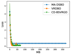
(a) Training loss

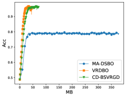
(b) Test accuracy

Figure 1: The training loss function value and test accuracy versus the communication cost (MB).

4.2 Synthetic Data

We first construct a synthetic dataset to evaluate our algorithm. Specifically, on the $k$-th worker, we generate the synthetic dataset with a noisy linear model: $y=\text{sign}(w^{T}x+0.1b)$, where $w\in\mathbb{R}^{200}$ and $b\in\mathbb{R}$ are drawn from standard Gaussian distributions, $x\in\mathbb{R}^{200}$ is drawn from a Gaussian distribution when $k\%2=0$, otherwise it is drawn from a Chi-square distribution where the number of degrees of freedom is $k$. Both the training and validation sets are generated in this way, while $x$ in the testing set is generated with the Gaussian distribution. In our experiments, we use eight workers where each worker has $6,250$ training samples and validation samples, as well as $1,000$ testing samples. Additionally, we use a linear graph to connect these workers.

We compare our algorithm with VRDBO [14], which is the most communication-efficient baseline algorithm under the homogeneous setting, and MA-DSBO [3], which is the most communication-efficient algorithm under the heterogeneous setting. As for the hyperparameter, we set $\epsilon$ to $0.01$ so that the learning rate of MA-DSBO is $0.01$ according to Theorem 3.3 in [3], and the learning rate of VRDBO and our algorithm is set to $0.1$ in terms of the corresponding theoretical results. $\alpha_{i}$ is tuned such that $\alpha_{i}\eta^{2}=1$ and $\beta_{i}$ is set to $1$ for both VRDBO and our algorithm. As for MA-DSBO, the number of iterations for the lower-level update and the Hessian-inverse-vector product update is set to $10$. Furthermore, the batch size of all algorithms is set to $100$, and the number of iterations is set to $2,000$.

In Figure 1(a), we show the lower-level loss function value (without the regularization term) versus the communicated megabytes (MB). Obviously, compared with MA-DSBO, our algorithm is more communication-efficient, which confirms the correctness of our theoretical result. Moreover, our algorithm can converge to a much smaller loss function value than MA-DSBO, which further confirms the effectiveness of our algorithm. It is worth noting that VRDBO has a smaller communication cost because it only communicates $x$ and $y$. In Figure 1(b), we report the test accuracy versus the communication cost, which further confirms the communication efficiency of our algorithm. Moreover, our algorithm can achieve a much better accuracy than MA-DSBO.

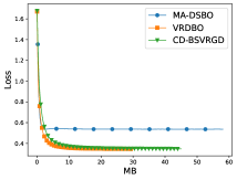
(a) a9a

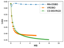
(b) ijcnn1

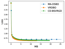
(c) covtype

Figure 2: The training loss function value versus the communication cost (MB).

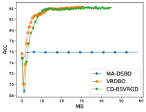
(a) a9a

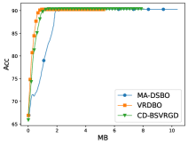
(b) ijcnn1

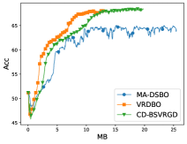
(c) covtype

Figure 3: The test accuracy versus the communication cost (MB).

4.3 Real-World Data

To further demonstrate the performance of our algorithm, we use three real-world LIBSVM datasets : a9a, ijcnn1, covtype. For each dataset, we randomly select $10\%$ samples as the test set, $70\%$ of the left samples as the training set, and the others as validation set. The other experimental settings regarding hyperparameters are same as the prior experiment.

In Figure 2, we plot the training loss function value versus the number of communicated megabytes. Note that we only show the first 500 iterations for MA-DSBO rather than all 2,000 iterations to make the comparison clearer. Similarly, we can find that our CD-BSVRGD algorithm is much more communication-efficient and can converge to a smaller function value than MA-DSBO. In Figure 3, we show the test accuracy versus the communication cost. It can still be observed that our algorithm is more communication-efficient in terms of the test accuracy. All these observations confirm the effectiveness of our algorithm.

5 Conclusion

In this paper, we studied how to improve the communication complexity of decentralized bilevel optimization algorithms under the heterogeneous setting. In particular, to reduce the communication rounds in each iteration, we proposed to employ the variance-reduced gradient descent on each worker to estimate the Hessian-inverse-vector product. As a result, our algorithm can reduce the communication rounds in each iteration and also reduce the cost in each round. Our theoretical analysis shows that our algorithm can achieve a much faster convergence rate than existing algorithms and can achieve linear speedup regarding the number of workers. The extensive experimental results confirm the efficacy of our algorithm.

Appendix A Proof of Theorem 1

At first, we introduce the following terminologies for convergence analysis.

$$\delta_{t}^{\hat{\mathcal{G}}_{F}}(X_{t},Y_{t},Z_{t})=[\hat{\mathcal{G}}_{F}^{(1)}(x_{t}^{(1)},y_{t}^{(1)},z_{t}^{(1)}),\hat{\mathcal{G}}_{F}^{(2)}(x_{t}^{(2)},y_{t}^{(2)},z_{t}^{(2)}),\cdots,\hat{\mathcal{G}}_{F}^{(K)}(x_{t}^{(K)},y_{t}^{(K)},z_{t}^{(K)})]\ ,$$ (A.1)

$$\delta_{t}^{\hat{\mathcal{G}}_{h}}(X_{t},Y_{t},Z_{t})=[\hat{\mathcal{G}}_{h}^{(1)}(x_{t}^{(1)},y_{t}^{(1)},z_{t}^{(1)}),\hat{\mathcal{G}}_{h}^{(2)}(x_{t}^{(2)},y_{t}^{(2)},z_{t}^{(2)}),\cdots,\hat{\mathcal{G}}_{h}^{(K)}(x_{t}^{(K)},y_{t}^{(K)},z_{t}^{(K)})]\ ,$$

$$\delta_{t}^{g}(X_{t},Y_{t})=[\nabla_{y}g^{(1)}(x_{t}^{(1)},y_{t}^{(1)}),\nabla_{y}g^{(2)}(x_{t}^{(2)},y_{t}^{(2)}),\cdots,\nabla_{y}g^{(K)}(x_{t}^{(K)},y_{t}^{(K)})]\ ,$$

Lemma 2.

[15] Under Assumptions 1-5, we have

$$\|\nabla F^{(k)}(x_{1})-{\nabla}F^{(k)}(x_{2})\|\leq{L}_{F}\|x_{1}-x_{2}\|\ ,$$ (A.2)

$$\|y^{*}(x_{1})-y^{*}(x_{2})\|\leq L_{y}\|x_{1}-x_{2}\|\ ,$$

where ${L}_{F}=(1+\frac{c_{g_{xy}}}{\mu})(\ell_{f_{x}}+\frac{\ell_{f_{y}}c_{g_{xy}}}{\mu}+\frac{c_{f_{y}}\ell_{g_{xy}}}{\mu}+\frac{\ell_{g_{yy}}c_{f_{y}}c_{g_{xy}}}{\mu^{2}})$, $L_{y}=\frac{c_{g_{xy}}}{\mu}$.

Lemma 3.

Under Assumptions 1-5, we have

$$\|z^{*}(x)\|\leq\frac{c_{f_{y}}}{\mu}\ , \|z^{*}(x_{1})-z^{*}(x_{2})\|\leq L_{z}\|x_{1}-x_{2}\|\ ,$$ (A.3)

where $L_{z}=(\frac{\ell_{f_{y}}}{\mu}+\frac{c_{f_{y}}\ell_{g_{yy}}}{\mu^{2}})(1+L_{y})$.

Proof.

According to the definition of $z^{*}(x)$, it is easy to know

$$\|z^{*}(x)\|=\left\|\left[\nabla_{22}^{2}g(x,y^{*}(x))\right]^{-1}\nabla_{2}{f(x,y^{*}(x))}\right\|\leq\frac{c_{f_{y}}}{\mu}\ .$$ (A.4)

As for the second inequality, we have

$$\quad\|z^{*}(x_{1})-z^{*}(x_{2})\|$$ (A.5)

$$=\|\left[\nabla_{22}^{2}g(x_{1},y^{*}(x_{1}))\right]^{-1}\nabla_{2}{f(x_{1},y^{*}(x_{1}))}-\left[\nabla_{22}^{2}g(x_{2},y^{*}(x_{2}))\right]^{-1}\nabla_{2}{f(x_{2},y^{*}(x_{2}))}\|$$

$$\leq\|\left[\nabla_{22}^{2}g(x_{1},y^{*}(x_{1}))\right]^{-1}\nabla_{2}{f(x_{1},y^{*}(x_{1}))}-\left[\nabla_{22}^{2}g(x_{1},y^{*}(x_{1}))\right]^{-1}\nabla_{2}{f(x_{2},y^{*}(x_{2}))}\|$$

$$\quad+\|\left[\nabla_{22}^{2}g(x_{1},y^{*}(x_{1}))\right]^{-1}\nabla_{2}{f(x_{2},y^{*}(x_{2}))}-\left[\nabla_{22}^{2}g(x_{2},y^{*}(x_{2}))\right]^{-1}\nabla_{2}{f(x_{2},y^{*}(x_{2}))}\|$$

$$\leq\frac{\ell_{f_{y}}}{\mu}(1+L_{y})\|x_{1}-x_{2}\|+\frac{c_{f_{y}}\ell_{g_{yy}}}{\mu^{2}}(1+L_{y})\|x_{1}-x_{2}\|$$

$$=(\frac{\ell_{f_{y}}}{\mu}+\frac{c_{f_{y}}\ell_{g_{yy}}}{\mu^{2}})(1+L_{y})\|x_{1}-x_{2}\|\ .$$

∎

Lemma 4.

Under Assumptions 1-5, we have

$$\|\nabla F(\bar{x}_{t})-\frac{1}{K}\delta^{\hat{\mathcal{G}}_{F}}(X_{t},Y_{t},Z_{t})\mathbf{1}\|^{2}\leq 6(\ell_{f_{x}}^{2}+\frac{c_{f_{y}}^{2}\ell_{g_{xy}}^{2}}{\mu^{2}})\|y^{*}(\bar{x}_{t})-y_{t}\|^{2}+6c_{g_{xy}}^{2}\|z^{*}(\bar{x}_{t})-\bar{z}_{t}\|^{2}$$ (A.6)

$$\quad+6(\ell_{f_{x}}^{2}+\frac{c_{f_{y}}^{2}\ell_{g_{xy}}^{2}}{\mu^{2}})\frac{1}{K}\|X_{t}-\bar{X}_{t}\|_{F}^{2}+6(\ell_{f_{x}}^{2}+\frac{c_{f_{y}}^{2}\ell_{g_{xy}}^{2}}{\mu^{2}})\frac{1}{K}\|Y_{t}-\bar{Y}_{t}\|_{F}^{2}+6c_{g_{xy}}^{2}\frac{1}{K}\|Z_{t}-\bar{Z}_{t}\|^{2}\ .$$

Proof.

$$\quad\|\nabla F(\bar{x}_{t})-\frac{1}{K}\delta^{\hat{\mathcal{G}}_{F}}(X_{t},Y_{t},Z_{t})\mathbf{1}\|^{2}$$ (A.7)

$$=\|\frac{1}{K}\sum_{k=1}^{K}\nabla_{1}f^{(k)}(\bar{x}_{t},y^{*}(\bar{x}_{t}))-\frac{1}{K}\sum_{k=1}^{K}\nabla_{12}^{2}g^{(k)}(\bar{x}_{t},y^{*}(\bar{x}_{t}))z^{*}(\bar{x}_{t})$$

$$\quad-\frac{1}{K}\sum_{k=1}^{K}\nabla_{1}{f^{(k)}({x}_{t}^{(k)},{y}_{t}^{(k)})}+\frac{1}{K}\sum_{k=1}^{K}\nabla_{12}^{2}g^{(k)}({x}_{t}^{(k)},{y}_{t}^{(k)})z_{t}^{(k)}\|^{2}$$

$$\leq 6\|\frac{1}{K}\sum_{k=1}^{K}\nabla_{1}f^{(k)}(\bar{x}_{t},y^{*}(\bar{x}_{t}))-\frac{1}{K}\sum_{k=1}^{K}\nabla_{1}f^{(k)}(\bar{x}_{t},\bar{y}_{t})\|^{2}+6\|\frac{1}{K}\sum_{k=1}^{K}\nabla_{1}f^{(k)}(\bar{x}_{t},\bar{y}_{t})-\frac{1}{K}\sum_{k=1}^{K}\nabla_{1}{f^{(k)}({x}_{t}^{(k)},{y}_{t}^{(k)})}\|^{2}$$

$$\quad+6\|-\frac{1}{K}\sum_{k=1}^{K}\nabla_{12}^{2}g^{(k)}(\bar{x}_{t},y^{*}(\bar{x}_{t}))z^{*}(\bar{x}_{t})+\frac{1}{K}\sum_{k=1}^{K}\nabla_{12}^{2}g^{(k)}(\bar{x}_{t},y^{*}(\bar{x}_{t}))\bar{z}_{t}\|^{2}$$

$$\quad+6\|-\frac{1}{K}\sum_{k=1}^{K}\nabla_{12}^{2}g^{(k)}(\bar{x}_{t},y^{*}(\bar{x}_{t}))\bar{z}_{t}+\frac{1}{K}\sum_{k=1}^{K}\nabla_{12}^{2}g^{(k)}(\bar{x}_{t},\bar{y}_{t})\bar{z}_{t}\|^{2}$$

$$\quad+6\|-\frac{1}{K}\sum_{k=1}^{K}\nabla_{12}^{2}g^{(k)}(\bar{x}_{t},\bar{y}_{t})\bar{z}_{t}+\frac{1}{K}\sum_{k=1}^{K}\nabla_{12}^{2}g^{(k)}(\bar{x}_{t},\bar{y}_{t})z_{t}^{(k)}\|^{2}$$

$$\quad+6\|-\frac{1}{K}\sum_{k=1}^{K}\nabla_{12}^{2}g^{(k)}(\bar{x}_{t},\bar{y}_{t})z_{t}^{(k)}+\frac{1}{K}\sum_{k=1}^{K}\nabla_{12}^{2}g^{(k)}({x}_{t}^{(k)},{y}_{t}^{(k)})z_{t}^{(k)}\|^{2}$$

$$\leq 6(\ell_{f_{x}}^{2}+\frac{c_{f_{y}}^{2}\ell_{g_{xy}}^{2}}{\mu^{2}})\|y^{*}(\bar{x}_{t})-y_{t}\|^{2}+6c_{g_{xy}}^{2}\|z^{*}(\bar{x}_{t})-\bar{z}_{t}\|^{2}$$

$$\quad+6(\ell_{f_{x}}^{2}+\frac{c_{f_{y}}^{2}\ell_{g_{xy}}^{2}}{\mu^{2}})\frac{1}{K}\sum_{k=1}^{K}\|{x}_{t}^{(k)}-\bar{x}_{t}\|^{2}+6(\ell_{f_{x}}^{2}+\frac{c_{f_{y}}^{2}\ell_{g_{xy}}^{2}}{\mu^{2}})\frac{1}{K}\sum_{k=1}^{K}\|{y}_{t}^{(k)}-\bar{y}_{t}\|^{2}+6c_{g_{xy}}^{2}\frac{1}{K}\sum_{k=1}^{K}\|{z}_{t}^{(k)}-\bar{z}_{t}\|^{2}\ .$$

∎

Lemma 5.

Under Assumptions 1-5, if $\eta\leq\frac{1}{2\beta_{1}L_{F}}$, we have

$$F(\bar{x}_{t+1})\leq F(\bar{x}_{t})-\frac{\beta_{1}\eta}{2}\|\nabla F(\bar{x}_{t})\|^{2}-\frac{\beta_{1}\eta}{4}\|\bar{u}_{t}\|^{2}$$ (A.8)

$$\quad+12\beta_{1}\eta\Big{(}\ell_{f_{x}}^{2}+\frac{c_{f_{y}}^{2}\ell_{g_{xy}}^{2}}{\mu^{2}}\Big{)}\|y^{*}(\bar{x}_{t})-\bar{y}_{t}\|^{2}+12\beta_{1}\eta c_{g_{xy}}^{2}\|z^{*}(\bar{x}_{t})-\bar{z}_{t}\|^{2}$$

$$\quad+12\beta_{1}\eta(\ell_{f_{x}}^{2}+\frac{c_{f_{y}}^{2}\ell_{g_{xy}}^{2}}{\mu^{2}})\frac{1}{K}\|{X}_{t}^{(k)}-\bar{X}_{t}\|_{F}^{2}+12\beta_{1}\eta(\ell_{f_{x}}^{2}+\frac{c_{f_{y}}^{2}\ell_{g_{xy}}^{2}}{\mu^{2}})\frac{1}{K}\|{Y}_{t}^{(k)}-\bar{Y}_{t}\|_{F}^{2}$$

$$\quad+12\beta_{1}\eta c_{g_{xy}}^{2}\frac{1}{K}\|{Z}_{t}-\bar{Z}_{t}\|_{F}^{2}+2\beta_{1}\eta\|\frac{1}{K}\delta^{\hat{\mathcal{G}}_{F}}(X_{t},Y_{t},Z_{t})\mathbf{1}-\frac{1}{K}{U}_{t}\mathbf{1}\|^{2}$$

Proof.

$$F(\bar{x}_{t+1})\leq F(\bar{x}_{t})+\langle\nabla F(\bar{x}_{t}),\bar{x}_{t+1}-\bar{x}_{t}\rangle+\frac{L_{F}}{2}\|\bar{x}_{t+1}-\bar{x}_{t}\|^{2}$$ (A.9)

$$=F(\bar{x}_{t})-\beta_{1}\eta\langle\nabla F(\bar{x}_{t}),{u}_{t}\rangle+\frac{\beta_{1}^{2}\eta^{2}L_{F}}{2}\|\bar{u}_{t}\|^{2}$$

$$=F(\bar{x}_{t})-\frac{\beta_{1}\eta}{2}\|\nabla F(\bar{x}_{t})\|^{2}-\frac{\beta_{1}\eta}{2}\|\bar{u}_{t}\|^{2}+\frac{\beta_{1}\eta}{2}\|\nabla F(\bar{x}_{t})-\bar{u}_{t}\|^{2}+\frac{\beta_{1}^{2}\eta^{2}L_{F}}{2}\|\bar{u}_{t}\|^{2}$$

$$\leq F(\bar{x}_{t})-\frac{\beta_{1}\eta}{2}\|\nabla F(\bar{x}_{t})\|^{2}-\frac{\beta_{1}\eta}{4}\|\bar{u}_{t}\|^{2}+\frac{\beta_{1}\eta}{2}\|\nabla F(\bar{x}_{t})-\bar{u}_{t}\|^{2}$$

$$\leq F(\bar{x}_{t})-\frac{\beta_{1}\eta}{2}\|\nabla F(\bar{x}_{t})\|^{2}-\frac{\beta_{1}\eta}{4}\|\bar{u}_{t}\|^{2}+\beta_{1}\eta\|\frac{1}{K}\delta^{\hat{\mathcal{G}}_{F}}(X_{t},Y_{t},Z_{t})\mathbf{1}-\frac{1}{K}{U}_{t}\mathbf{1}\|^{2}$$

$$\quad+\beta_{1}\eta\|\nabla F(\bar{x}_{t})-\frac{1}{K}\delta^{\hat{\mathcal{G}}_{F}}(X_{t},Y_{t},Z_{t})\mathbf{1}\|^{2}\ .$$

where the fourth step follows from $\eta\leq\frac{1}{2\beta_{1}L_{F}}$. Then, due to Lemma 4, we can get

$$F(\bar{x}_{t+1})\leq F(\bar{x}_{t})-\frac{\beta_{1}\eta}{2}\|\nabla F(\bar{x}_{t})\|^{2}-\frac{\beta_{1}\eta}{4}\|\bar{u}_{t}\|^{2}$$ (A.10)

$$\quad+12\beta_{1}\eta\Big{(}\ell_{f_{x}}^{2}+\frac{c_{f_{y}}^{2}\ell_{g_{xy}}^{2}}{\mu^{2}}\Big{)}\|y^{*}(\bar{x}_{t})-\bar{y}_{t}\|^{2}+12\beta_{1}\eta c_{g_{xy}}^{2}\|z^{*}(\bar{x}_{t})-\bar{z}_{t}\|^{2}$$

$$\quad+12\beta_{1}\eta(\ell_{f_{x}}^{2}+\frac{c_{f_{y}}^{2}\ell_{g_{xy}}^{2}}{\mu^{2}})\frac{1}{K}\|{X}_{t}^{(k)}-\bar{X}_{t}\|_{F}^{2}+12\beta_{1}\eta(\ell_{f_{x}}^{2}+\frac{c_{f_{y}}^{2}\ell_{g_{xy}}^{2}}{\mu^{2}})\frac{1}{K}\|{Y}_{t}^{(k)}-\bar{Y}_{t}\|_{F}^{2}$$

$$\quad+12\beta_{1}\eta c_{g_{xy}}^{2}\frac{1}{K}\|{Z}_{t}-\bar{Z}_{t}\|_{F}^{2}+2\beta_{1}\eta\|\frac{1}{K}\delta^{\hat{\mathcal{G}}_{F}}(X_{t},Y_{t},Z_{t})\mathbf{1}-\frac{1}{K}{U}_{t}\mathbf{1}\|^{2}\ .$$

∎

Lemma 6.

Under Assumptions 1-5, if $\eta\leq\frac{1}{\beta_{3}\mu}$, we have

$$\quad\mathbb{E}[\|\bar{z}_{t+1}-z^{*}(\bar{{x}}_{t+1})\|^{2}]\leq(1-\frac{\eta\beta_{3}\mu}{8})\mathbb{E}[\|\bar{z}_{t}-z^{*}(\bar{x}_{t})\|^{2}]+\frac{9\eta\beta_{3}}{\mu}\Big{(}\frac{c_{f_{y}}^{2}\ell_{g_{yy}}^{2}}{\mu^{2}}+\ell_{f_{y}}^{2}\Big{)}\mathbb{E}[\|\bar{y}_{t}-y^{*}(\bar{x}_{t})\|^{2}]+\frac{9\eta\beta_{1}^{2}L_{z}^{2}}{\beta_{3}\mu}\mathbb{E}[\|\bar{u}_{t}\|^{2}]$$ (A.11)

$$\quad+\frac{9\eta\beta_{3}^{2}}{4}\frac{1}{K}\mathbb{E}[\|R_{t}-\bar{R}_{t}\|_{F}^{2}]+\Big{(}\frac{70\eta\beta_{3}}{\mu}\ell_{g_{y}}^{2}+\frac{9}{4}\Big{)}\frac{1}{K}\mathbb{E}[\|{Z}_{t}-\bar{Z}_{t}\|_{F}^{2}]+\frac{70\eta\beta_{3}}{\mu}\Big{(}\frac{c_{f_{y}}^{2}\ell_{g_{yy}}^{2}}{\mu^{2}}+\ell_{f_{y}}^{2}\Big{)}\frac{1}{K}\mathbb{E}[\|\bar{X}_{t}-{X}_{t}\|_{F}^{2}]$$

$$\quad+\frac{70\eta\beta_{3}}{\mu}\Big{(}\frac{c_{f_{y}}^{2}\ell_{g_{yy}}^{2}}{\mu^{2}}+\ell_{f_{y}}^{2}\Big{)}\frac{1}{K}\mathbb{E}[\|\bar{Y}_{t}-{Y}_{t}\|_{F}^{2}]+\frac{25\eta\beta_{3}}{\mu}\mathbb{E}[\|\frac{1}{K}\delta^{\hat{\mathcal{G}}_{h}}({X}_{t},{Y}_{t},{Z}_{t})\mathbf{1}-\frac{1}{K}{W}_{t}\mathbf{1}\|^{2}]\ .$$

Proof.

At first, we have

$$\quad\|\bar{z}_{t}-\eta\beta_{3}\hat{\mathcal{G}}_{h}(\bar{x}_{t},\bar{y}_{t},\bar{z}_{t})-z^{*}(\bar{x}_{t})+\eta\beta_{3}\nabla_{z}h(\bar{x}_{t},z^{*}(\bar{x}_{t}))\|^{2}$$ (A.12)

$$=\|\bar{z}_{t}-\eta\beta_{3}(\nabla_{22}^{2}g(\bar{x}_{t},\bar{y}_{t})\bar{z}_{t}-\nabla_{2}f(\bar{x}_{t},\bar{y}_{t}))-z^{*}(\bar{x}_{t})+\eta\beta_{3}(\nabla_{22}^{2}g(\bar{x}_{t},y^{*}(\bar{x}_{t}))z^{*}(\bar{x}_{t})-\nabla_{2}{f(\bar{x}_{t},y^{*}(\bar{x}_{t}))})\|^{2}$$

$$\leq(1+a)\|(I-\eta\beta_{3}\nabla_{22}^{2}g(\bar{x}_{t},\bar{y}_{t}))\bar{z}_{t}-(I-\eta\beta_{3}\nabla_{22}^{2}g(\bar{x}_{t},\bar{y}_{t}))z^{*}(\bar{x}_{t})\|^{2}$$

$$\quad+2(1+1/a)\|(I-\eta\beta_{3}\nabla_{22}^{2}g(\bar{x}_{t},\bar{y}_{t}))z^{*}(\bar{x}_{t})-(I-\eta\beta_{3}\nabla_{22}^{2}g(\bar{x}_{t},y^{*}(\bar{x}_{t})))z^{*}(\bar{x}_{t})\|^{2}$$

$$\quad+2(1+1/a)\|\eta\beta_{3}(\nabla_{2}f(\bar{x}_{t},\bar{y}_{t})-\nabla_{2}{f(\bar{x}_{t},y^{*}(\bar{x}_{t}))})\|^{2}$$

$$\leq(1+a)(1-\eta\beta_{3}\mu)^{2}\|\bar{z}_{t}-z^{*}(\bar{x}_{t})\|^{2}+2\eta^{2}\beta_{3}^{2}\frac{c_{f_{y}}^{2}\ell_{g_{yy}}^{2}}{\mu^{2}}(1+1/a)\|\bar{y}_{t}-y^{*}(\bar{x}_{t})\|^{2}$$

$$\quad+2\eta^{2}\beta_{3}^{2}\ell_{f_{y}}^{2}(1+1/a)\|\bar{y}_{t}-y^{*}(\bar{x}_{t})\|^{2}$$

$$\leq(1+a)(1-\eta\beta_{3}\mu)\|\bar{z}_{t}-z^{*}(\bar{x}_{t})\|^{2}+2\eta^{2}\beta_{3}^{2}\Big{(}\frac{c_{f_{y}}^{2}\ell_{g_{yy}}^{2}}{\mu^{2}}+\ell_{f_{y}}^{2}\Big{)}(1+1/a)\|\bar{y}_{t}-y^{*}(\bar{x}_{t})\|^{2}$$

$$\leq(1-\frac{\eta\beta_{3}\mu}{2})\|\bar{z}_{t}-z^{*}(\bar{x}_{t})\|^{2}+\frac{6\eta\beta_{3}}{\mu}\Big{(}\frac{c_{f_{y}}^{2}\ell_{g_{yy}}^{2}}{\mu^{2}}+\ell_{f_{y}}^{2}\Big{)}\|\bar{y}_{t}-y^{*}(\bar{x}_{t})\|^{2}\ ,$$

where the third step follows from Assumptions 1-4, the last step follows from $a=\frac{\eta\beta_{3}\mu}{2}$ and $\eta\leq\frac{1}{\beta_{3}\mu}$.

Then, we have

$$\quad\|\bar{z}_{t}-\eta\beta_{3}\bar{r}_{t}-z^{*}(\bar{x}_{t})\|^{2}$$ (A.13)

$$=\|\bar{z}_{t}-\eta\beta_{3}\bar{w}_{t}-z^{*}(\bar{x}_{t})\|^{2}$$

$$=\|\bar{z}_{t}-\eta\beta_{3}\hat{\mathcal{G}}_{h}(\bar{x}_{t},\bar{y}_{t},\bar{z}_{t})+\eta\beta_{3}\hat{\mathcal{G}}_{h}(\bar{x}_{t},\bar{y}_{t},\bar{z}_{t})-\eta\beta_{3}\bar{w}_{t}-z^{*}(\bar{x}_{t})\|^{2}$$

$$\leq(1+a)\|\bar{z}_{t}-\eta\beta_{3}\hat{\mathcal{G}}_{h}(\bar{x}_{t},\bar{y}_{t},\bar{z}_{t})-z^{*}(\bar{x}_{t})\|^{2}+(1+1/a)\eta^{2}\beta_{3}^{2}\|\hat{\mathcal{G}}_{h}(\bar{x}_{t},\bar{y}_{t},\bar{z}_{t})-\frac{1}{K}{W}_{t}\mathbf{1}\|^{2}$$

$$\leq(1+a)\|\bar{z}_{t}-\eta\beta_{3}\hat{\mathcal{G}}_{h}(\bar{x}_{t},\bar{y}_{t},\bar{z}_{t})-z^{*}(\bar{x}_{t})+\eta\beta_{3}\nabla_{z}h(\bar{x}_{t},z^{*}(\bar{x}_{t}))\|^{2}$$

$$\quad+2(1+1/a)\eta^{2}\beta_{3}^{2}\|\hat{\mathcal{G}}_{h}(\bar{x}_{t},\bar{y}_{t},\bar{z}_{t})-\frac{1}{K}\delta^{\hat{\mathcal{G}}_{h}}({X}_{t},{Y}_{t},{Z}_{t})\mathbf{1}\|^{2}$$

$$\quad+2(1+1/a)\eta^{2}\beta_{3}^{2}\|\frac{1}{K}\delta^{\hat{\mathcal{G}}_{h}}({X}_{t},{Y}_{t},{Z}_{t})\mathbf{1}-\frac{1}{K}{W}_{t}\mathbf{1}\|^{2}$$

$$\leq(1+a)(1-\frac{\eta\beta_{3}\mu}{2})\|\bar{z}_{t}-z^{*}(\bar{x}_{t})\|^{2}+(1+a)\frac{6\eta\beta_{3}}{\mu}\Big{(}\frac{c_{f_{y}}^{2}\ell_{g_{yy}}^{2}}{\mu^{2}}+\ell_{f_{y}}^{2}\Big{)}\|\bar{y}_{t}-y^{*}(\bar{x}_{t})\|^{2}$$

$$\quad+2(1+1/a)\eta^{2}\beta_{3}^{2}\|\hat{\mathcal{G}}_{h}(\bar{x}_{t},\bar{y}_{t},\bar{z}_{t})-\frac{1}{K}\delta^{\hat{\mathcal{G}}_{h}}({X}_{t},{Y}_{t},{Z}_{t})\mathbf{1}\|^{2}$$

$$\quad+2(1+1/a)\eta^{2}\beta_{3}^{2}\|\frac{1}{K}\delta^{\hat{\mathcal{G}}_{h}}({X}_{t},{Y}_{t},{Z}_{t})\mathbf{1}-\frac{1}{K}{W}_{t}\mathbf{1}\|^{2}$$

$$\leq(1-\frac{\eta\beta_{3}\mu}{4})\|\bar{z}_{t}-z^{*}(\bar{x}_{t})\|^{2}+\frac{8\eta\beta_{3}}{\mu}\Big{(}\frac{c_{f_{y}}^{2}\ell_{g_{yy}}^{2}}{\mu^{2}}+\ell_{f_{y}}^{2}\Big{)}\|\bar{y}_{t}-y^{*}(\bar{x}_{t})\|^{2}$$

$$\quad+\frac{20\eta\beta_{3}}{\mu}\|\hat{\mathcal{G}}_{h}(\bar{x}_{t},\bar{y}_{t},\bar{z}_{t})-\frac{1}{K}\delta^{\hat{\mathcal{G}}_{h}}({X}_{t},{Y}_{t},{Z}_{t})\mathbf{1}\|^{2}+\frac{20\eta\beta_{3}}{\mu}\|\frac{1}{K}\delta^{\hat{\mathcal{G}}_{h}}({X}_{t},{Y}_{t},{Z}_{t})\mathbf{1}-\frac{1}{K}{W}_{t}\mathbf{1}\|^{2}$$

$$\leq(1-\frac{\eta\beta_{3}\mu}{4})\|\bar{z}_{t}-z^{*}(\bar{x}_{t})\|^{2}+\frac{8\eta\beta_{3}}{\mu}\Big{(}\frac{c_{f_{y}}^{2}\ell_{g_{yy}}^{2}}{\mu^{2}}+\ell_{f_{y}}^{2}\Big{)}\|\bar{y}_{t}-y^{*}(\bar{x}_{t})\|^{2}$$

$$\quad+\frac{60\eta\beta_{3}}{\mu}\ell_{g_{y}}^{2}\frac{1}{K}\|{Z}_{t}-\bar{Z}_{t}\|_{F}^{2}+\frac{60\eta\beta_{3}}{\mu}\Big{(}\frac{c_{f_{y}}^{2}\ell_{g_{yy}}^{2}}{\mu^{2}}+\ell_{f_{y}}^{2}\Big{)}\frac{1}{K}\|\bar{X}_{t}-{X}_{t}\|_{F}^{2}+\frac{60\eta\beta_{3}}{\mu}\Big{(}\frac{c_{f_{y}}^{2}\ell_{g_{yy}}^{2}}{\mu^{2}}+\ell_{f_{y}}^{2}\Big{)}\frac{1}{K}\|\bar{Y}_{t}-{Y}_{t}\|_{F}^{2}$$

$$\quad+\frac{20\eta\beta_{3}}{\mu}\|\frac{1}{K}\delta^{\hat{\mathcal{G}}_{h}}({X}_{t},{Y}_{t},{Z}_{t})\mathbf{1}-\frac{1}{K}{W}_{t}\mathbf{1}\|^{2}\ ,$$

where the third step follows from $\nabla_{z}h(\bar{x}_{t},z^{*}(\bar{x}_{t}))=0$, the fourth step follows from Eq. (A.12), the fifth step follows from $a=\frac{\eta\beta_{3}\mu}{4}$ and $\eta\leq\frac{1}{\beta_{3}\mu}$, and the last step follows from the following inequality.

$$\quad\|\hat{\mathcal{G}}_{h}(\bar{x}_{t},\bar{y}_{t},\bar{z}_{t})-\frac{1}{K}\delta^{\hat{\mathcal{G}}_{h}}({X}_{t},{Y}_{t},{Z}_{t})\mathbf{1}\|^{2}$$ (A.14)

$$\leq\frac{1}{K}\sum_{k=1}^{K}\|\nabla_{22}^{2}g^{(k)}(\bar{x}_{t},\bar{y}_{t})\bar{z}_{t}-\nabla_{2}{f^{(k)}(\bar{x}_{t},\bar{y}_{t})}-\nabla_{22}^{2}g^{(k)}({x}_{t}^{(k)},{y}_{t}^{(k)}){z}_{t}^{(k)}+\nabla_{2}{f^{(k)}({x}_{t}^{(k)},{y}_{t}^{(k)})}\|^{2}$$

$$\leq 3\frac{1}{K}\sum_{k=1}^{K}\|\nabla_{22}^{2}g^{(k)}(\bar{x}_{t},\bar{y}_{t})\bar{z}_{t}-\nabla_{22}^{2}g^{(k)}(\bar{x}_{t},\bar{y}_{t}){z}_{t}^{(k)}\|^{2}$$

$$\quad+3\frac{1}{K}\sum_{k=1}^{K}\|\nabla_{22}^{2}g^{(k)}(\bar{x}_{t},\bar{y}_{t}){z}_{t}^{(k)}-\nabla_{22}^{2}g^{(k)}({x}_{t}^{(k)},{y}_{t}^{(k)}){z}_{t}^{(k)}\|^{2}$$

$$\quad+3\frac{1}{K}\sum_{k=1}^{K}\|-\nabla_{2}{f^{(k)}(\bar{x}_{t},\bar{y}_{t})}+\nabla_{2}{f^{(k)}({x}_{t}^{(k)},{y}_{t}^{(k)})}\|^{2}$$

$$\leq 3\ell_{g_{y}}^{2}\frac{1}{K}\|{Z}_{t}-\bar{Z}_{t}\|_{F}^{2}+3\Big{(}\frac{c_{f_{y}}^{2}\ell_{g_{yy}}^{2}}{\mu^{2}}+\ell_{f_{y}}^{2}\Big{)}\frac{1}{K}\|\bar{X}_{t}-{X}_{t}\|_{F}^{2}+3\Big{(}\frac{c_{f_{y}}^{2}\ell_{g_{yy}}^{2}}{\mu^{2}}+\ell_{f_{y}}^{2}\Big{)}\frac{1}{K}\|\bar{Y}_{t}-{Y}_{t}\|_{F}^{2}\ ,$$

where the last step follows from Assumptions 1-4. Then, we have

$$\quad\|\bar{z}_{t+1}-z^{*}(\bar{x}_{t+1})\|^{2}\leq(1+a)\|\bar{z}_{t+1}-z^{*}(\bar{x}_{t})\|^{2}+(1+1/a)\|z^{*}(\bar{x}_{t+1})-z^{*}(\bar{x}_{t})\|^{2}$$ (A.15)

$$\leq(1+a)\frac{2}{K}\|Z_{t}-\bar{Z}_{t}\|_{F}^{2}+(1+a)2\eta\beta_{3}^{2}\frac{1}{K}\|R_{t}-\bar{R}_{t}\|_{F}^{2}$$

$$\quad+(1+a)\|\bar{z}_{t}-\eta\beta_{3}\bar{r}_{t}-z^{*}(\bar{x}_{t})\|^{2}+(1+1/a)\|z^{*}(\bar{x}_{t+1})-z^{*}(\bar{x}_{t})\|^{2}$$

$$\leq(1+a)\frac{2}{K}\|Z_{t}-\bar{Z}_{t}\|_{F}^{2}+(1+a)2\eta\beta_{3}^{2}\frac{1}{K}\|R_{t}-\bar{R}_{t}\|_{F}^{2}+(1+1/a)L_{z}^{2}\|\bar{x}_{t+1}-\bar{x}_{t}\|^{2}$$

$$\quad+(1+a)(1-\frac{\eta\beta_{3}\mu}{4})\|\bar{z}_{t}-z^{*}(\bar{x}_{t})\|^{2}+(1+a)\frac{8\eta\beta_{3}}{\mu}\Big{(}\frac{c_{f_{y}}^{2}\ell_{g_{yy}}^{2}}{\mu^{2}}+\ell_{f_{y}}^{2}\Big{)}\|\bar{y}_{t}-y^{*}(\bar{x}_{t})\|^{2}$$

$$\quad+(1+a)\frac{60\eta\beta_{3}}{\mu}\ell_{g_{y}}^{2}\frac{1}{K}\|{Z}_{t}-\bar{Z}_{t}\|_{F}^{2}+(1+a)\frac{60\eta\beta_{3}}{\mu}\Big{(}\frac{c_{f_{y}}^{2}\ell_{g_{yy}}^{2}}{\mu^{2}}+\ell_{f_{y}}^{2}\Big{)}\frac{1}{K}\|\bar{X}_{t}-{X}_{t}\|_{F}^{2}$$

$$\quad+(1+a)\frac{60\eta\beta_{3}}{\mu}\Big{(}\frac{c_{f_{y}}^{2}\ell_{g_{yy}}^{2}}{\mu^{2}}+\ell_{f_{y}}^{2}\Big{)}\frac{1}{K}\|\bar{Y}_{t}-{Y}_{t}\|_{F}^{2}+(1+a)\frac{20\eta\beta_{3}}{\mu}\|\frac{1}{K}\sum_{k=1}^{K}\hat{\mathcal{G}}_{h}^{(k)}({x}_{t}^{(k)},{y}_{t}^{(k)},{z}_{t}^{(k)})-\frac{1}{K}{W}_{t}\mathbf{1}\|^{2}$$

$$\leq(1-\frac{\eta\beta_{3}\mu}{8})\|\bar{z}_{t}-z^{*}(\bar{x}_{t})\|^{2}+\frac{9\eta\beta_{3}}{\mu}\Big{(}\frac{c_{f_{y}}^{2}\ell_{g_{yy}}^{2}}{\mu^{2}}+\ell_{f_{y}}^{2}\Big{)}\|\bar{y}_{t}-y^{*}(\bar{x}_{t})\|^{2}+\frac{9\eta\beta_{1}^{2}L_{z}^{2}}{\beta_{3}\mu}\|\bar{u}_{t}\|^{2}+\frac{9\eta\beta_{3}^{2}}{4}\frac{1}{K}\|R_{t}-\bar{R}_{t}\|_{F}^{2}$$

$$\quad+\Big{(}\frac{70\eta\beta_{3}}{\mu}\ell_{g_{y}}^{2}+\frac{9}{4}\Big{)}\frac{1}{K}\|{Z}_{t}-\bar{Z}_{t}\|_{F}^{2}+\frac{70\eta\beta_{3}}{\mu}\Big{(}\frac{c_{f_{y}}^{2}\ell_{g_{yy}}^{2}}{\mu^{2}}+\ell_{f_{y}}^{2}\Big{)}\frac{1}{K}\|\bar{X}_{t}-{X}_{t}\|_{F}^{2}+\frac{70\eta\beta_{3}}{\mu}\Big{(}\frac{c_{f_{y}}^{2}\ell_{g_{yy}}^{2}}{\mu^{2}}+\ell_{f_{y}}^{2}\Big{)}\frac{1}{K}\|\bar{Y}_{t}-{Y}_{t}\|_{F}^{2}$$

$$\quad+\frac{25\eta\beta_{3}}{\mu}\|\frac{1}{K}\sum_{k=1}^{K}\hat{\mathcal{G}}_{h}^{(k)}({x}_{t}^{(k)},{y}_{t}^{(k)},{z}_{t}^{(k)})-\frac{1}{K}{W}_{t}\mathbf{1}\|^{2}\ ,$$

where the second step follows from Eq. (A.16), the third step follows from Eq. (A.12), the last step follows from $a=\frac{\eta\beta_{3}\mu}{8}$ and $\eta\leq\frac{1}{\beta_{3}\mu}$.

$$\quad\|\bar{z}_{t+1}-z^{*}(\bar{x}_{t})\|^{2}$$ (A.16)

$$\leq\frac{1}{K}\sum_{k=1}^{K}\|z_{t+1}^{(k)}-z^{*}(\bar{x}_{t})\|^{2}$$

$$=\frac{1}{K}\sum_{k=1}^{K}\|(1-\eta)z_{t}^{(k)}+\eta\mathcal{P}[\sum_{j\in\mathcal{N}_{k}}w_{kj}z_{t}^{(j)}-\beta_{3}r^{(k)}_{t}]-z^{*}(\bar{x}_{t})\|^{2}$$

$$\leq\frac{1}{K}\sum_{k=1}^{K}\|\eta\sum_{j\in\mathcal{N}_{k}}w_{kj}z_{t}^{(j)}-\eta\beta_{3}r^{(k)}_{t}+(1-\eta)z_{t}^{(k)}-z^{*}(\bar{x}_{t})\|^{2}$$

$$\leq\frac{1}{K}\sum_{k=1}^{K}\|\eta\sum_{j\in\mathcal{N}_{k}}w_{kj}z_{t}^{(j)}-\eta\bar{z}_{t}+\eta\bar{z}_{t}-\eta\beta_{3}r^{(k)}_{t}+\eta\beta_{3}\bar{r}_{t}-\eta\beta_{3}\bar{r}_{t}+(1-\eta)z_{t}^{(k)}-(1-\eta)\bar{z}_{t}+(1-\eta)\bar{z}_{t}-z^{*}(\bar{x}_{t})\|^{2}$$

$$=\frac{1}{K}\sum_{k=1}^{K}\|\eta\sum_{j\in\mathcal{N}_{k}}w_{kj}z_{t}^{(j)}-\eta\bar{z}_{t}-\eta\beta_{3}r^{(k)}_{t}+\eta\beta_{3}\bar{r}_{t}+(1-\eta)z_{t}^{(k)}-(1-\eta)\bar{z}_{t}\|^{2}+\|\bar{z}_{t}-\eta\beta_{3}\bar{r}_{t}-z^{*}(\bar{x}_{t})\|^{2}$$

$$=\frac{1}{K}\|\eta(WZ_{t}-\bar{Z}_{t}-\beta_{3}R_{t}+\beta_{3}\bar{R}_{t})+(1-\eta)(Z_{t}-\bar{Z}_{t})\|_{F}^{2}+\|\bar{z}_{t}-\eta\beta_{3}\bar{r}_{t}-z^{*}(\bar{x}_{t})\|^{2}$$

$$\leq\frac{1}{K}\eta\|WZ_{t}-\bar{Z}_{t}-\beta_{3}R_{t}+\beta_{3}\bar{R}_{t}\|_{F}^{2}+(1-\eta)\frac{1}{K}\|Z_{t}-\bar{Z}_{t}\|_{F}^{2}+\|\bar{z}_{t}-\eta\beta_{3}\bar{r}_{t}-z^{*}(\bar{x}_{t})\|^{2}$$

$$\leq 2\eta\frac{1}{K}\|WZ_{t}-\bar{Z}_{t}\|_{F}^{2}+2\eta\beta_{3}^{2}\frac{1}{K}\|R_{t}-\bar{R}_{t}\|_{F}^{2}+(1-\eta)\frac{1}{K}\|Z_{t}-\bar{Z}_{t}\|_{F}^{2}+\|\bar{z}_{t}-\eta\beta_{3}\bar{r}_{t}-z^{*}(\bar{x}_{t})\|^{2}$$

$$\leq 2\eta\lambda^{2}\frac{1}{K}\|Z_{t}-\bar{Z}_{t}\|_{F}^{2}+2\eta\beta_{3}^{2}\frac{1}{K}\|R_{t}-\bar{R}_{t}\|_{F}^{2}+(1-\eta)\frac{1}{K}\|Z_{t}-\bar{Z}_{t}\|_{F}^{2}+\|\bar{z}_{t}-\eta\beta_{3}\bar{r}_{t}-z^{*}(\bar{x}_{t})\|^{2}$$

$$\leq 2\frac{1}{K}\|Z_{t}-\bar{Z}_{t}\|_{F}^{2}+2\eta\beta_{3}^{2}\frac{1}{K}\|R_{t}-\bar{R}_{t}\|_{F}^{2}+\|\bar{z}_{t}-\eta\beta_{3}\bar{r}_{t}-z^{*}(\bar{x}_{t})\|^{2}\ ,$$

where the third step follows from that $z_{t}^{(k)}$ and $z^{*}(\bar{x}_{t})$ satisfy the constraint and the projection is non-expansive, the fifth step follows from $\frac{1}{K}\sum_{k=1}^{K}(\eta\sum_{j\in\mathcal{N}_{k}}w_{kj}z_{t}^{(j)}-\eta\bar{z}_{t}-\eta\beta_{3}r^{(k)}_{t}+\eta\beta_{3}\bar{r}_{t}+(1-\eta)z_{t}^{(k)}-(1-\eta)\bar{z}_{t})=0$, the fourth to last step follows from $\|x+y\|^{2}\leq(1+a)\|x\|^{2}+(1+1/a)\|y\|^{2}$ with $a=\frac{\eta}{1-\eta}$, and the last step follows from $\eta<1$ and $\lambda<1$.

∎

Lemma 7.

Under Assumptions 1-5, if $\beta_{2}\leq\frac{1}{6\ell_{g_{y}}}$, we have

$$\quad\mathbb{E}[\|\bar{{y}}_{t+1}-{y}^{*}(\bar{{x}}_{t+1})\|^{2}]\leq(1-\frac{\beta_{2}\eta\mu}{4})\mathbb{E}[\|\bar{{y}}_{t}-{y}^{*}(\bar{{x}}_{t})\|^{2}]-\frac{3\eta\beta_{2}^{2}}{4}\mathbb{E}[\|\bar{v}_{t}\|^{2}]+\frac{25\eta\beta_{1}^{2}L_{y}^{2}}{6\beta_{2}\mu}\mathbb{E}[\|\bar{u}_{t}\|^{2}]$$ (A.17)

$$\quad+\frac{25\beta_{2}\eta\ell_{g_{y}}^{2}}{3\mu}\frac{1}{K}\mathbb{E}[\|\bar{X}_{t}-{X}_{t}\|_{F}^{2}]+\frac{25\beta_{2}\eta\ell_{g_{y}}^{2}}{3\mu}\frac{1}{K}\mathbb{E}[\|\bar{Y}_{t}-{Y}_{t}\|_{F}^{2}]$$

$$\quad+\frac{25\beta_{2}\eta}{3\mu}\mathbb{E}[\|\frac{1}{K}\delta^{g}({X}_{t},{Y}_{t})\mathbf{1}-\frac{1}{K}{V}_{t}\mathbf{1}\|^{2}]\ .$$

This lemma can be proved by following Eq.(52) in [14]. Therefore, we omit its detailed proof.

Lemma 8.

Under Assumptions 1-5, we have the following two inequalities:

$$\quad\mathbb{E}[\|\frac{1}{K}\delta^{\hat{\mathcal{G}}_{F}}(X_{t},Y_{t},Z_{t})\mathbf{1}-\frac{1}{K}U_{t}\mathbf{1}\|^{2}]$$ (A.18)

$$\leq(1-\alpha_{1}\eta^{2})\mathbb{E}[\|\frac{1}{K}\delta^{\hat{\mathcal{G}}_{F}}(X_{t-1},Y_{t-1},Z_{t-1})\mathbf{1}-\frac{1}{K}U_{t-1}\mathbf{1}\|^{2}]$$

$$\quad+6(\ell_{f_{x}}^{2}+\frac{c_{f_{y}}^{2}\ell_{g_{xy}}^{2}}{\mu^{2}})\frac{1}{K^{2}}\mathbb{E}[\|X_{t}-X_{t-1}\|_{F}^{2}]+6(\ell_{f_{x}}^{2}+\frac{c_{f_{y}}^{2}\ell_{g_{xy}}^{2}}{\mu^{2}})\frac{1}{K^{2}}\mathbb{E}[\|Y_{t}-Y_{t-1}\|_{F}^{2}]$$

$$\quad+6c_{g_{xy}}^{2}\frac{1}{K^{2}}\mathbb{E}[\|Z_{t}-Z_{t-1}\|_{F}^{2}]+4\alpha_{1}^{2}\eta^{4}(1+\frac{c_{f_{y}}^{2}}{\mu^{2}})\sigma^{2}\frac{1}{K}\ ,$$

and

$$\quad\frac{1}{K}\mathbb{E}[\|\delta^{\hat{\mathcal{G}}_{F}}(X_{t},Y_{t},Z_{t})-U_{t}\|_{F}^{2}]$$ (A.19)

$$\leq(1-\alpha_{1}\eta^{2})\frac{1}{K}\mathbb{E}[\|\delta^{\hat{\mathcal{G}}_{F}}(X_{t-1},Y_{t-1},Z_{t-1})-U_{t-1}\|_{F}^{2}]$$

$$\quad+6(\ell_{f_{x}}^{2}+\frac{c_{f_{y}}^{2}\ell_{g_{xy}}^{2}}{\mu^{2}})\frac{1}{K}\mathbb{E}[\|X_{t}-X_{t-1}\|_{F}^{2}]$$

$$\quad+6(\ell_{f_{x}}^{2}+\frac{c_{f_{y}}^{2}\ell_{g_{xy}}^{2}}{\mu^{2}})\frac{1}{K}\mathbb{E}[\|Y_{t}-Y_{t-1}\|_{F}^{2}]$$

$$\quad+6c_{g_{xy}}^{2}\frac{1}{K}\mathbb{E}[\|Z_{t}-Z_{t-1}\|_{F}^{2}]+4\alpha_{1}^{2}\eta^{4}(1+\frac{c_{f_{y}}^{2}}{\mu^{2}})\sigma^{2}\ .$$

Proof.

Eq. (A.18) can be proved as follows:

$$\quad\mathbb{E}[\|(\delta^{\hat{\mathcal{G}}_{F}}(X_{t},Y_{t},Z_{t})-U_{t})\frac{1}{K}\mathbf{1}\|^{2}]$$ (A.20)

$$=\mathbb{E}[\|\Big{(}(1-\alpha_{1}\eta^{2})(\delta^{\hat{\mathcal{G}}_{F}}(X_{t-1},Y_{t-1},Z_{t-1})-U_{t-1})$$

$$\quad+(1-\alpha_{1}\eta^{2})(\delta^{\hat{\mathcal{G}}_{F}}(X_{t},Y_{t},Z_{t};\hat{\xi}_{t})-\delta^{\hat{\mathcal{G}}_{F}}(X_{t},Y_{t},Z_{t};\hat{\xi}_{t})-\delta^{\hat{\mathcal{G}}_{F}}(X_{t},Y_{t},Z_{t})+\delta^{\hat{\mathcal{G}}_{F}}(X_{t-1},Y_{t-1},Z_{t-1}))$$

$$\quad+\alpha_{1}\eta^{2}(\delta^{\hat{\mathcal{G}}_{F}}(X_{t},Y_{t},Z_{t};\hat{\xi}_{t})-\delta^{\hat{\mathcal{G}}_{F}}(X_{t},Y_{t},Z_{t}))\Big{)}\frac{1}{K}\mathbf{1}\|^{2}]$$

$$\leq(1-\alpha_{1}\eta^{2})^{2}\mathbb{E}[\|(\delta^{\hat{\mathcal{G}}_{F}}(X_{t-1},Y_{t-1},Z_{t-1})-U_{t-1})\frac{1}{K}\mathbf{1}\|^{2}]$$

$$\quad+2(1-\alpha_{1}\eta^{2})^{2}\frac{1}{K^{2}}\mathbb{E}[\|\delta^{\hat{\mathcal{G}}_{F}}(X_{t},Y_{t},Z_{t};\hat{\xi}_{t})-\delta^{\hat{\mathcal{G}}_{F}}(X_{t-1},Y_{t-1},Z_{t-1};\hat{\xi}_{t})-\delta^{\hat{\mathcal{G}}_{F}}(X_{t},Y_{t},Z_{t})+\delta^{\hat{\mathcal{G}}_{F}}(X_{t-1},Y_{t-1},Z_{t-1})\|_{F}^{2}]$$

$$\quad+2\alpha_{1}^{2}\eta^{4}\frac{1}{K^{2}}\mathbb{E}[\|\delta^{\hat{\mathcal{G}}_{F}}(X_{t},Y_{t},Z_{t};\hat{\xi}_{t})-\delta^{\hat{\mathcal{G}}_{F}}(X_{t},Y_{t},Z_{t})\|_{F}^{2}]$$

$$\leq(1-\alpha_{1}\eta^{2})\mathbb{E}[\|(\delta^{\hat{\mathcal{G}}_{F}}(X_{t-1},Y_{t-1},Z_{t-1})-U_{t-1})\frac{1}{K}\mathbf{1}\|^{2}]$$

$$\quad+2\frac{1}{K^{2}}\mathbb{E}[\|\delta^{\hat{\mathcal{G}}_{F}}(X_{t},Y_{t},Z_{t};\hat{\xi}_{t})-\delta^{\hat{\mathcal{G}}_{F}}(X_{t-1},Y_{t-1},Z_{t-1};\hat{\xi}_{t})\|_{F}^{2}]$$

$$\quad+2\alpha_{1}^{2}\eta^{4}\frac{1}{K^{2}}\mathbb{E}[\|\delta^{\hat{\mathcal{G}}_{F}}(X_{t},Y_{t},Z_{t};\hat{\xi}_{t})-\delta^{\hat{\mathcal{G}}_{F}}(X_{t},Y_{t},Z_{t})\|_{F}^{2}]$$

$$\leq(1-\alpha_{1}\eta^{2})\mathbb{E}[\|(\delta^{\hat{\mathcal{G}}_{F}}(X_{t-1},Y_{t-1},Z_{t-1})-U_{t-1})\frac{1}{K}\mathbf{1}\|^{2}]$$

$$\quad+6(\ell_{f_{x}}^{2}+\frac{c_{f_{y}}^{2}\ell_{g_{xy}}^{2}}{\mu^{2}})\frac{1}{K^{2}}\mathbb{E}[\|X_{t}-X_{t-1}\|_{F}^{2}]+6(\ell_{f_{x}}^{2}+\frac{c_{f_{y}}^{2}\ell_{g_{xy}}^{2}}{\mu^{2}})\frac{1}{K^{2}}\mathbb{E}[\|Y_{t}-Y_{t-1}\|_{F}^{2}]$$

$$\quad+6c_{g_{xy}}^{2}\frac{1}{K^{2}}\mathbb{E}[\|Z_{t}-Z_{t-1}\|_{F}^{2}]+4\alpha_{1}^{2}\eta^{4}(1+\frac{c_{f_{y}}^{2}}{\mu^{2}})\sigma^{2}\frac{1}{K}\ ,$$

where the last step follows from the following two inequalities:

$$\quad\mathbb{E}[\|\delta^{\hat{\mathcal{G}}_{F}}(X_{t},Y_{t},Z_{t};\hat{\xi}_{t})-\delta^{\hat{\mathcal{G}}_{F}}(X_{t},Y_{t},Z_{t})\|_{F}^{2}]$$ (A.21)

$$=\sum_{k=1}^{K}\mathbb{E}[\|\hat{\mathcal{G}}_{F}^{(k)}(x_{t}^{(k)},y_{t}^{(k)},z_{t}^{(k)};\hat{\xi}_{t}^{(k)})-\hat{\mathcal{G}}_{F}^{(k)}(x_{t}^{(k)},y_{t}^{(k)},z_{t}^{(k)})\|^{2}]$$

$$=\sum_{k=1}^{K}\mathbb{E}[\|\nabla_{1}{f^{(k)}(x_{t}^{(k)},y_{t}^{(k)};{\xi}_{t}^{(k)})}-\nabla_{12}^{2}g^{(k)}(x_{t}^{(k)},y_{t}^{(k)};{\zeta}_{t}^{(k)})z_{t}^{(k)}$$

$$\quad-\nabla_{1}{f^{(k)}(x_{t}^{(k)},y_{t}^{(k)})}+\nabla_{12}^{2}g^{(k)}(x_{t}^{(k)},y_{t}^{(k)})z_{t}^{(k)}\|^{2}]$$

$$\leq 2(1+\frac{c_{f_{y}}^{2}}{\mu^{2}})\sigma^{2}K\ ,$$

and

$$\quad\mathbb{E}[\|\delta^{\hat{\mathcal{G}}_{F}}(X_{t},Y_{t},Z_{t};\hat{\xi}_{t})-\delta^{\hat{\mathcal{G}}_{F}}(X_{t-1},Y_{t-1},Z_{t-1};\hat{\xi}_{t})\|_{F}^{2}]$$ (A.22)

$$=\sum_{k=1}^{K}\mathbb{E}[\|\nabla_{1}{f^{(k)}(x_{t}^{(k)},y_{t}^{(k)};{\xi}_{t}^{(k)})}-\nabla_{1}{f^{(k)}(x_{t-1}^{(k)},y_{t-1}^{(k)};{\xi}_{t}^{(k)})}$$

$$\quad-\nabla_{12}^{2}g^{(k)}(x_{t}^{(k)},y_{t}^{(k)};{\zeta}_{t}^{(k)})z_{t}^{(k)}+\nabla_{12}^{2}g^{(k)}(x_{t}^{(k)},y_{t}^{(k)};{\zeta}_{t}^{(k)})z_{t-1}^{(k)}$$

$$\quad-\nabla_{12}^{2}g^{(k)}(x_{t}^{(k)},y_{t}^{(k)};{\zeta}_{t}^{(k)})z_{t-1}^{(k)}+\nabla_{12}^{2}g^{(k)}(x_{t-1}^{(k)},y_{t-1}^{(k)};{\zeta}_{t}^{(k)})z_{t-1}^{(k)}\|^{2}]$$

$$\leq 3(\ell_{f_{x}}^{2}+\frac{c_{f_{y}}^{2}\ell_{g_{xy}}^{2}}{\mu^{2}})\mathbb{E}[\|X_{t}-X_{t-1}\|_{F}^{2}]+3(\ell_{f_{x}}^{2}+\frac{c_{f_{y}}^{2}\ell_{g_{xy}}^{2}}{\mu^{2}})\mathbb{E}[\|Y_{t}-Y_{t-1}\|_{F}^{2}]$$

$$\quad+3c_{g_{xy}}^{2}\mathbb{E}[\|Z_{t}-Z_{t-1}\|_{F}^{2}]\ .$$

Eq. (A.19) can be proved by following the above proof so that we omit the detailed steps.

∎

Lemma 9.

Under Assumptions 1-5, we have the following two inequalities:

$$\mathbb{E}[\|(\delta^{g}(X_{t},Y_{t})-V_{t})\frac{1}{K}\mathbf{1}\|^{2}]\leq(1-\alpha_{2}\eta^{2})\mathbb{E}[\|(\delta^{g}(X_{t-1},Y_{t-1})-V_{t-1})\frac{1}{K}\mathbf{1}\|^{2}]$$ (A.23)

$$\quad+2\ell_{g_{y}}^{2}\frac{1}{K^{2}}\mathbb{E}[\|X_{t}-X_{t-1}\|_{F}^{2}]+2\ell_{g_{y}}^{2}\frac{1}{K^{2}}\mathbb{E}[\|Y_{t}-Y_{t-1}\|_{F}^{2}]+2\alpha_{2}^{2}\eta^{4}\sigma^{2}\frac{1}{K}\ ,$$

and

$$\frac{1}{K}\mathbb{E}[\|\delta^{g}(X_{t},Y_{t})-V_{t}\|_{F}^{2}]\leq(1-\alpha_{2}\eta^{2})\frac{1}{K}\mathbb{E}[\|\delta^{g}(X_{t-1},Y_{t-1})-V_{t-1}\|_{F}^{2}]$$ (A.24)

$$\quad+2\ell_{g_{y}}^{2}\frac{1}{K}\mathbb{E}[\|X_{t}-X_{t-1}\|_{F}^{2}]+2\ell_{g_{y}}^{2}\frac{1}{K}\mathbb{E}[\|Y_{t}-Y_{t-1}\|_{F}^{2}]+2\alpha_{2}^{2}\eta^{4}\sigma^{2}\ .$$

Proof.

Eq. (A.23) can be proved as follows:

$$\quad\mathbb{E}[\|(\delta^{g}(X_{t},Y_{t})-V_{t})\frac{1}{K}\mathbf{1}\|^{2}]$$ (A.25)

$$=\mathbb{E}[\|\Big{(}(1-\alpha_{2}\eta^{2})(\delta^{g}(X_{t-1},Y_{t-1})-V_{t-1})$$

$$\quad+(1-\alpha_{2}\eta^{2})(\delta^{g}(X_{t},Y_{t};{\zeta}_{t})-\delta^{g}(X_{t},Y_{t};{\zeta}_{t})-\delta^{g}(X_{t},Y_{t})+\delta^{g}(X_{t-1},Y_{t-1}))$$

$$\quad+\alpha_{2}\eta^{2}(\delta^{g}(X_{t},Y_{t};{\zeta}_{t})-\delta^{g}(X_{t},Y_{t}))\Big{)}\frac{1}{K}\mathbf{1}\|^{2}]$$

$$\leq(1-\alpha_{2}\eta^{2})^{2}\mathbb{E}[\|(\delta^{g}(X_{t-1},Y_{t-1})-V_{t-1})\frac{1}{K}\mathbf{1}\|^{2}]$$

$$\quad+2(1-\alpha_{2}\eta^{2})^{2}\frac{1}{K^{2}}\mathbb{E}[\|\delta^{g}(X_{t},Y_{t};{\zeta}_{t})-\delta^{g}(X_{t-1},Y_{t-1};{\zeta}_{t})-\delta^{g}(X_{t},Y_{t})+\delta^{g}(X_{t-1},Y_{t-1})\|_{F}^{2}]$$

$$\quad+2\alpha_{2}^{2}\eta^{4}\frac{1}{K^{2}}\mathbb{E}[\|\delta^{g}(X_{t},Y_{t};{\zeta}_{t})-\delta^{g}(X_{t},Y_{t})\|_{F}^{2}]$$

$$\leq(1-\alpha_{2}\eta^{2})\mathbb{E}[\|(\delta^{g}(X_{t-1},Y_{t-1})-V_{t-1})\frac{1}{K}\mathbf{1}\|^{2}]$$

$$\quad+2\frac{1}{K^{2}}\mathbb{E}[\|\delta^{g}(X_{t},Y_{t};{\zeta}_{t})-\delta^{g}(X_{t-1},Y_{t-1};{\zeta}_{t})\|_{F}^{2}]+2\alpha_{2}^{2}\eta^{4}\frac{1}{K^{2}}\mathbb{E}[\|\delta^{g}(X_{t},Y_{t};{\zeta}_{t})-\delta^{g}(X_{t},Y_{t})\|_{F}^{2}]$$

$$\leq(1-\alpha_{2}\eta^{2})\mathbb{E}[\|(\delta^{g}(X_{t-1},Y_{t-1})-V_{t-1})\frac{1}{K}\mathbf{1}\|^{2}]$$

$$\quad+2\ell_{g_{y}}^{2}\frac{1}{K^{2}}\mathbb{E}[\|X_{t}-X_{t-1}\|_{F}^{2}]+2\ell_{g_{y}}^{2}\frac{1}{K^{2}}\mathbb{E}[\|Y_{t}-Y_{t-1}\|_{F}^{2}]+2\alpha_{2}^{2}\eta^{4}\sigma^{2}\frac{1}{K}\ .$$

Eq. (A.24) can be proved by following the above proof so that we omit the detailed steps. ∎

Lemma 10.

Under Assumptions 1-5, we have the following two inequalities:

$$\mathbb{E}[\|(\delta^{\hat{\mathcal{G}}_{h}}(X_{t},Y_{t},Z_{t})-W_{t})\frac{1}{K}\mathbf{1}\|^{2}]\leq(1-\alpha_{3}\eta^{2})\mathbb{E}[\|(\delta^{\hat{\mathcal{G}}_{h}}(X_{t-1},Y_{t-1},Z_{t-1})-W_{t-1})\frac{1}{K}\mathbf{1}\|^{2}]$$ (A.26)

$$\quad+6(\frac{c_{f_{y}}^{2}\ell_{g_{yy}}^{2}}{\mu^{2}}+\ell_{f_{y}}^{2})\frac{1}{K^{2}}\mathbb{E}[\|X_{t}-X_{t-1}\|_{F}^{2}]+6(\frac{c_{f_{y}}^{2}\ell_{g_{yy}}^{2}}{\mu^{2}}+\ell_{f_{y}}^{2})\frac{1}{K^{2}}\mathbb{E}[\|Y_{t}-Y_{t-1}\|_{F}^{2}]$$

$$\quad+6\ell_{g_{y}}^{2}\frac{1}{K^{2}}\mathbb{E}[\|Z_{t}-Z_{t-1}\|_{F}^{2}]+4\alpha_{3}^{2}\eta^{4}(1+\frac{c_{f_{y}}^{2}}{\mu^{2}})\sigma^{2}\frac{1}{K}\ ,$$

and

$$\frac{1}{K}\mathbb{E}[\|\delta^{\hat{\mathcal{G}}_{h}}(X_{t},Y_{t},Z_{t})-W_{t}\|^{2}]\leq(1-\alpha_{3}\eta^{2})\frac{1}{K}\mathbb{E}[\|\delta^{\hat{\mathcal{G}}_{h}}(X_{t-1},Y_{t-1},Z_{t-1})-W_{t-1}\|^{2}]$$ (A.27)

$$\quad+6(\frac{c_{f_{y}}^{2}\ell_{g_{yy}}^{2}}{\mu^{2}}+\ell_{f_{y}}^{2})\frac{1}{K}\mathbb{E}[\|X_{t}-X_{t-1}\|_{F}^{2}]+6(\frac{c_{f_{y}}^{2}\ell_{g_{yy}}^{2}}{\mu^{2}}+\ell_{f_{y}}^{2})\frac{1}{K}\mathbb{E}[\|Y_{t}-Y_{t-1}\|_{F}^{2}]$$

$$\quad+6\ell_{g_{y}}^{2}\frac{1}{K}\mathbb{E}[\|Z_{t}-Z_{t-1}\|_{F}^{2}]+4\alpha_{3}^{2}\eta^{4}(1+\frac{c_{f_{y}}^{2}}{\mu^{2}})\sigma^{2}\ .$$

Proof.

Eq. (A.26) can be proved as follows:

$$\quad\mathbb{E}[\|(\delta^{\hat{\mathcal{G}}_{h}}(X_{t},Y_{t},Z_{t})-W_{t})\frac{1}{K}\mathbf{1}\|^{2}]$$ (A.28)

$$=\mathbb{E}[\|\Big{(}(1-\alpha_{3}\eta^{2})(\delta^{\hat{\mathcal{G}}_{h}}(X_{t-1},Y_{t-1},Z_{t-1})-W_{t-1})$$

$$\quad+(1-\alpha_{3}\eta^{2})(\delta^{\hat{\mathcal{G}}_{h}}(X_{t},Y_{t},Z_{t};\hat{\xi}_{t})-\delta^{\hat{\mathcal{G}}_{h}}(X_{t},Y_{t},Z_{t};\hat{\xi}_{t})-\delta^{\hat{\mathcal{G}}_{h}}(X_{t},Y_{t},Z_{t})+\delta^{\hat{\mathcal{G}}_{h}}(X_{t-1},Y_{t-1},Z_{t-1}))$$

$$\quad+\alpha_{3}\eta^{2}(\delta^{\hat{\mathcal{G}}_{h}}(X_{t},Y_{t},Z_{t};\hat{\xi}_{t})-\delta^{\hat{\mathcal{G}}_{h}}(X_{t},Y_{t},Z_{t}))\Big{)}\frac{1}{K}\mathbf{1}\|^{2}]$$

$$\leq(1-\alpha_{3}\eta^{2})^{2}\mathbb{E}[\|(\delta^{\hat{\mathcal{G}}_{h}}(X_{t-1},Y_{t-1},Z_{t-1})-W_{t-1})\frac{1}{K}\mathbf{1}\|^{2}]$$

$$\quad+2(1-\alpha_{3}\eta^{2})^{2}\frac{1}{K^{2}}\mathbb{E}[\|\delta^{\hat{\mathcal{G}}_{h}}(X_{t},Y_{t},Z_{t};\hat{\xi}_{t})-\delta^{\hat{\mathcal{G}}_{h}}(X_{t-1},Y_{t-1},Z_{t-1};\hat{\xi}_{t})-\delta^{\hat{\mathcal{G}}_{h}}(X_{t},Y_{t},Z_{t})+\delta^{\hat{\mathcal{G}}_{h}}(X_{t-1},Y_{t-1},Z_{t-1})\|_{F}^{2}]$$

$$\quad+2\alpha_{3}^{2}\eta^{4}\frac{1}{K^{2}}\mathbb{E}[\|\delta^{\hat{\mathcal{G}}_{h}}(X_{t},Y_{t},Z_{t};\hat{\xi}_{t})-\delta^{\hat{\mathcal{G}}_{h}}(X_{t},Y_{t},Z_{t})\|_{F}^{2}]$$

$$\leq(1-\alpha_{3}\eta^{2})\mathbb{E}[\|(\delta^{\hat{\mathcal{G}}_{h}}(X_{t-1},Y_{t-1},Z_{t-1})-W_{t-1})\frac{1}{K}\mathbf{1}\|^{2}]$$

$$\quad+2\frac{1}{K^{2}}\mathbb{E}[\|\delta^{\hat{\mathcal{G}}_{h}}(X_{t},Y_{t},Z_{t};\hat{\xi}_{t})-\delta^{\hat{\mathcal{G}}_{h}}(X_{t-1},Y_{t-1},Z_{t-1};\hat{\xi}_{t})\|_{F}^{2}]+2\alpha_{3}^{2}\eta^{4}\frac{1}{K^{2}}\mathbb{E}[\|\delta^{\hat{\mathcal{G}}_{h}}(X_{t},Y_{t},Z_{t};\hat{\xi}_{t})-\delta^{\hat{\mathcal{G}}_{h}}(X_{t},Y_{t},Z_{t})\|_{F}^{2}]$$

$$\leq(1-\alpha_{3}\eta^{2})\mathbb{E}[\|(\delta^{\hat{\mathcal{G}}_{h}}(X_{t-1},Y_{t-1},Z_{t-1})-W_{t-1})\frac{1}{K}\mathbf{1}\|^{2}]$$

$$\quad+6(\frac{c_{f_{y}}^{2}\ell_{g_{yy}}^{2}}{\mu^{2}}+\ell_{f_{y}}^{2})\frac{1}{K^{2}}\mathbb{E}[\|X_{t}-X_{t-1}\|_{F}^{2}]+6(\frac{c_{f_{y}}^{2}\ell_{g_{yy}}^{2}}{\mu^{2}}+\ell_{f_{y}}^{2})\frac{1}{K^{2}}\mathbb{E}[\|Y_{t}-Y_{t-1}\|_{F}^{2}]$$

$$\quad+6\ell_{g_{y}}^{2}\frac{1}{K^{2}}\mathbb{E}[\|Z_{t}-Z_{t-1}\|_{F}^{2}]+4\alpha_{3}^{2}\eta^{4}(1+\frac{c_{f_{y}}^{2}}{\mu^{2}})\sigma^{2}\frac{1}{K}\ ,$$

where the last step follows from the following two inequalities:

$$\quad\mathbb{E}[\|\delta^{\hat{\mathcal{G}}_{h}}(X_{t},Y_{t},Z_{t};\hat{\xi}_{t})-\delta^{\hat{\mathcal{G}}_{h}}(X_{t-1},Y_{t-1},Z_{t-1};\hat{\xi}_{t})\|_{F}^{2}]$$ (A.29)

$$=\sum_{k=1}^{K}\mathbb{E}[\|\nabla_{22}^{2}g^{(k)}(x_{t}^{(k)},y_{t}^{(k)};\zeta_{t}^{(k)})z_{t}^{(k)}-\nabla_{2}{f^{(k)}(x_{t}^{(k)},y_{t}^{(k)};\xi_{t}^{(k)})}$$

$$\quad-\nabla_{22}^{2}g^{(k)}(x_{t-1}^{(k)},y_{t-1}^{(k)};\zeta_{t}^{(k)})z_{t-1}^{(k)}+\nabla_{2}{f^{(k)}(x_{t-1}^{(k)},y_{t-1}^{(k)};\xi_{t}^{(k)})}\|^{2}]$$

$$=\sum_{k=1}^{K}\mathbb{E}[\|\nabla_{22}^{2}g^{(k)}(x_{t}^{(k)},y_{t}^{(k)};\zeta_{t}^{(k)})z_{t}^{(k)}-\nabla_{22}^{2}g^{(k)}(x_{t-1}^{(k)},y_{t-1}^{(k)};\zeta_{t}^{(k)})z_{t}^{(k)}$$

$$\quad+\nabla_{22}^{2}g^{(k)}(x_{t-1}^{(k)},y_{t-1}^{(k)};\zeta_{t}^{(k)})z_{t}^{(k)}-\nabla_{22}^{2}g^{(k)}(x_{t-1}^{(k)},y_{t-1}^{(k)};\zeta_{t}^{(k)})z_{t-1}^{(k)}$$

$$\quad-\nabla_{2}{f^{(k)}(x_{t}^{(k)},y_{t}^{(k)};\xi_{t}^{(k)})}+\nabla_{2}{f^{(k)}(x_{t-1}^{(k)},y_{t-1}^{(k)};\xi_{t}^{(k)})}\|^{2}]$$

$$\leq 3(\frac{c_{f_{y}}^{2}\ell_{g_{yy}}^{2}}{\mu^{2}}+\ell_{f_{y}}^{2})\mathbb{E}[\|X_{t}-X_{t-1}\|_{F}^{2}]+3(\frac{c_{f_{y}}^{2}\ell_{g_{yy}}^{2}}{\mu^{2}}+\ell_{f_{y}}^{2})\mathbb{E}[\|Y_{t}-Y_{t-1}\|_{F}^{2}]$$

$$\quad+3\ell_{g_{y}}^{2}\mathbb{E}[\|Z_{t}-Z_{t-1}\|_{F}^{2}]\ ,$$

and

$$\mathbb{E}[\|\delta^{\hat{\mathcal{G}}_{h}}(X_{t},Y_{t},Z_{t};\hat{\xi}_{t})-\delta^{\hat{\mathcal{G}}_{h}}(X_{t},Y_{t},Z_{t})\|_{F}^{2}]$$ (A.30)

$$=\sum_{k=1}^{K}\mathbb{E}[\|\nabla_{22}^{2}g^{(k)}(x_{t}^{(k)},y_{t}^{(k)};\zeta_{t}^{(k)})z_{t}^{(k)}-\nabla_{2}{f^{(k)}(x_{t}^{(k)},y_{t}^{(k)};\xi_{t}^{(k)})}$$

$$\quad-\nabla_{22}^{2}g^{(k)}(x_{t}^{(k)},y_{t}^{(k)})z_{t}^{(k)}+\nabla_{2}{f^{(k)}(x_{t}^{(k)},y_{t}^{(k)})}\|^{2}]$$

$$\leq 2(1+\frac{c_{f_{y}}^{2}}{\mu^{2}})\sigma^{2}K\ .$$

Eq. (A.27) can be proved by following the above proof so that we omit the detailed steps.

∎

Lemma 11.

Under Assumptions 1-5, we have

$$\frac{1}{K}\mathbb{E}[\|P_{t}-\bar{P}_{t}\|_{F}^{2}]\leq\lambda\frac{1}{K}\mathbb{E}[\|P_{t-1}-\bar{P}_{t-1}\|_{F}^{2}]+\frac{3\alpha_{1}^{2}\eta^{4}}{1-\lambda}\frac{1}{K}\mathbb{E}[\|U_{t-1}-\delta^{\hat{\mathcal{G}}_{F}}(X_{t-1},Y_{t-1},Z_{t-1})\|_{F}^{2}]$$ (A.31)

$$\quad+(\ell_{f_{x}}^{2}+\frac{c_{f_{y}}^{2}\ell_{g_{xy}}^{2}}{\mu^{2}})\frac{9}{1-\lambda}\frac{1}{K}\mathbb{E}[\|X_{t}-X_{t-1}\|_{F}^{2}]+(\ell_{f_{x}}^{2}+\frac{c_{f_{y}}^{2}\ell_{g_{xy}}^{2}}{\mu^{2}})\frac{9}{1-\lambda}\frac{1}{K}\mathbb{E}[\|Y_{t}-Y_{t-1}\|_{F}^{2}]$$

$$\quad+c_{g_{xy}}^{2}\frac{9}{1-\lambda}\frac{1}{K}\mathbb{E}[\|Z_{t}-Z_{t-1}\|_{F}^{2}]+\frac{6\alpha_{1}^{2}\eta^{4}}{1-\lambda}(1+\frac{c_{f_{y}}^{2}}{\mu^{2}})\sigma^{2}\ .$$

Proof.

$$\quad\frac{1}{K}\mathbb{E}[\|P_{t}-\bar{P}_{t}\|_{F}^{2}]$$ (A.32)

$$=\frac{1}{K}\mathbb{E}[\|P_{t-1}E+U_{t}-U_{t-1}-\bar{P}_{t-1}-\bar{U}_{t}+\bar{U}_{t-1}\|_{F}^{2}]$$

$$\leq\frac{1}{K}\lambda\mathbb{E}[\|P_{t-1}-\bar{P}_{t-1}\|_{F}^{2}]+\frac{1}{1-\lambda}\frac{1}{K}\mathbb{E}[\|U_{t}-U_{t-1}-\bar{U}_{t}+\bar{U}_{t-1}\|_{F}^{2}]$$

$$\leq\lambda\frac{1}{K}\mathbb{E}[\|P_{t-1}-\bar{P}_{t-1}\|_{F}^{2}]+\frac{1}{1-\lambda}\frac{1}{K}\mathbb{E}[\|U_{t}-U_{t-1}\|_{F}^{2}]$$

$$=\lambda\frac{1}{K}\mathbb{E}[\|P_{t-1}-\bar{P}_{t-1}\|_{F}^{2}]$$

$$\quad+\frac{1}{1-\lambda}\frac{1}{K}\mathbb{E}[\|(1-\alpha_{1}\eta^{2})(U_{t-1}-\delta^{\hat{\mathcal{G}}_{F}}(X_{t-1},Y_{t-1},Z_{t-1};\hat{\xi}_{t}))+\delta^{\hat{\mathcal{G}}_{F}}(X_{t},Y_{t},Z_{t};\hat{\xi}_{t})-U_{t-1}\|_{F}^{2}]$$

$$=\lambda\frac{1}{K}\mathbb{E}[\|P_{t-1}-\bar{P}_{t-1}\|_{F}^{2}]$$

$$\quad+\frac{1}{1-\lambda}\frac{1}{K}\mathbb{E}[\|\delta^{\hat{\mathcal{G}}_{F}}(X_{t},Y_{t},Z_{t};\hat{\xi}_{t})-\delta^{\hat{\mathcal{G}}_{F}}(X_{t-1},Y_{t-1},Z_{t-1};\hat{\xi}_{t})-\alpha_{1}\eta^{2}(U_{t-1}-\delta^{\hat{\mathcal{G}}_{F}}(X_{t-1},Y_{t-1},Z_{t-1}))$$

$$\quad-\alpha_{1}\eta^{2}(\delta^{\hat{\mathcal{G}}_{F}}(X_{t-1},Y_{t-1},Z_{t-1})-\delta^{\hat{\mathcal{G}}_{F}}(X_{t-1},Y_{t-1},Z_{t-1};\hat{\xi}_{t}))\|_{F}^{2}]$$

$$\leq\lambda\frac{1}{K}\mathbb{E}[\|P_{t-1}-\bar{P}_{t-1}\|_{F}^{2}]+\frac{3}{1-\lambda}\frac{1}{K}\mathbb{E}[\|\delta^{\hat{\mathcal{G}}_{F}}(X_{t},Y_{t},Z_{t};\hat{\xi}_{t})-\delta^{\hat{\mathcal{G}}_{F}}(X_{t-1},Y_{t-1},Z_{t-1};\hat{\xi}_{t})\|_{F}^{2}]$$

$$\quad+\frac{3\alpha_{1}^{2}\eta^{4}}{1-\lambda}\frac{1}{K}\mathbb{E}[\|U_{t-1}-\delta^{\hat{\mathcal{G}}_{F}}(X_{t-1},Y_{t-1},Z_{t-1})\|_{F}^{2}]$$

$$\quad+\frac{3\alpha_{1}^{2}\eta^{4}}{1-\lambda}\frac{1}{K}\mathbb{E}[\|\delta^{\hat{\mathcal{G}}_{F}}(X_{t-1},Y_{t-1},Z_{t-1})-\delta^{\hat{\mathcal{G}}_{F}}(X_{t-1},Y_{t-1},Z_{t-1};\hat{\xi}_{t})\|_{F}^{2}]$$

$$\leq\lambda\frac{1}{K}\mathbb{E}[\|P_{t-1}-\bar{P}_{t-1}\|_{F}^{2}]+\frac{3\alpha_{1}^{2}\eta^{4}}{1-\lambda}\frac{1}{K}\mathbb{E}[\|U_{t-1}-\delta^{\hat{\mathcal{G}}_{F}}(X_{t-1},Y_{t-1},Z_{t-1})\|_{F}^{2}]$$

$$\quad+(\ell_{f_{x}}^{2}+\frac{c_{f_{y}}^{2}\ell_{g_{xy}}^{2}}{\mu^{2}})\frac{9}{1-\lambda}\frac{1}{K}\mathbb{E}[\|X_{t}-X_{t-1}\|_{F}^{2}]+(\ell_{f_{x}}^{2}+\frac{c_{f_{y}}^{2}\ell_{g_{xy}}^{2}}{\mu^{2}})\frac{9}{1-\lambda}\frac{1}{K}\mathbb{E}[\|Y_{t}-Y_{t-1}\|_{F}^{2}]$$

$$\quad+c_{g_{xy}}^{2}\frac{9}{1-\lambda}\frac{1}{K}\mathbb{E}[\|Z_{t}-Z_{t-1}\|_{F}^{2}]+\frac{6\alpha_{1}^{2}\eta^{4}}{1-\lambda}(1+\frac{c_{f_{y}}^{2}}{\mu^{2}})\sigma^{2}\ .$$

∎

Lemma 12.

Under Assumptions 1-5, we have

$$\quad\frac{1}{K}\mathbb{E}[\|R_{t}-\bar{R}_{t}\|_{F}^{2}]\leq\lambda\frac{1}{K}\mathbb{E}[\|R_{t-1}-\bar{R}_{t-1}\|_{F}^{2}]+\frac{3\alpha_{3}^{2}\eta^{4}}{1-\lambda}\frac{1}{K}\mathbb{E}[\|W_{t-1}-\delta^{\hat{\mathcal{G}}_{h}}(X_{t-1},Y_{t-1},Z_{t-1})\|_{F}^{2}]$$ (A.33)

$$\quad+(\ell_{f_{y}}^{2}+\frac{c_{f_{y}}^{2}\ell_{g_{yy}}^{2}}{\mu^{2}})\frac{9}{1-\lambda}\frac{1}{K}\mathbb{E}[\|X_{t}-X_{t-1}\|_{F}^{2}]+(\ell_{f_{y}}^{2}+\frac{c_{f_{y}}^{2}\ell_{g_{yy}}^{2}}{\mu^{2}})\frac{9}{1-\lambda}\frac{1}{K}\mathbb{E}[\|Y_{t}-Y_{t-1}\|_{F}^{2}]$$

$$\quad+\ell_{g_{y}}^{2}\frac{9}{1-\lambda}\frac{1}{K}\mathbb{E}[\|Z_{t}-Z_{t-1}\|_{F}^{2}]+\frac{6\alpha_{3}^{2}\eta^{4}}{1-\lambda}(1+\frac{c_{f_{y}}^{2}}{\mu^{2}})\sigma^{2}\ .$$

Proof.

$$\quad\frac{1}{K}\mathbb{E}[\|R_{t}-\bar{R}_{t}\|_{F}^{2}]=\frac{1}{K}\mathbb{E}[\|R_{t-1}E+W_{t}-W_{t-1}-\bar{R}_{t-1}-\bar{W}_{t}+\bar{W}_{t-1}\|_{F}^{2}]$$ (A.34)

$$\leq\frac{1}{K}\lambda\mathbb{E}[\|R_{t-1}-\bar{R}_{t-1}\|_{F}^{2}]+\frac{1}{1-\lambda}\frac{1}{K}\mathbb{E}[\|W_{t}-W_{t-1}-\bar{W}_{t}+\bar{W}_{t-1}\|_{F}^{2}]$$

$$\leq\lambda\frac{1}{K}\mathbb{E}[\|R_{t-1}-\bar{R}_{t-1}\|_{F}^{2}]+\frac{1}{1-\lambda}\frac{1}{K}\mathbb{E}[\|W_{t}-W_{t-1}\|_{F}^{2}]$$

$$=\lambda\frac{1}{K}\mathbb{E}[\|R_{t-1}-\bar{R}_{t-1}\|_{F}^{2}]+\frac{1}{1-\lambda}\frac{1}{K}\mathbb{E}[\|(1-\alpha_{3}\eta^{2})(W_{t-1}-\delta^{\hat{\mathcal{G}}_{h}}(X_{t-1},Y_{t-1},Z_{t-1};\hat{\xi}_{t}))+\delta^{\hat{\mathcal{G}}_{h}}(X_{t},Y_{t},Z_{t};\hat{\xi}_{t})-W_{t-1}\|_{F}^{2}]$$

$$=\lambda\frac{1}{K}\mathbb{E}[\|R_{t-1}-\bar{R}_{t-1}\|_{F}^{2}]+\frac{1}{1-\lambda}\frac{1}{K}\mathbb{E}[\|\delta^{\hat{\mathcal{G}}_{h}}(X_{t},Y_{t},Z_{t};\hat{\xi}_{t})-\delta^{\hat{\mathcal{G}}_{h}}(X_{t-1},Y_{t-1},Z_{t-1};\hat{\xi}_{t})$$

$$\quad-\alpha_{3}\eta^{2}(W_{t-1}-\delta^{\hat{\mathcal{G}}_{h}}(X_{t-1},Y_{t-1},Z_{t-1}))-\alpha_{3}\eta^{2}(\delta^{\hat{\mathcal{G}}_{h}}(X_{t-1},Y_{t-1},Z_{t-1})-\delta^{\hat{\mathcal{G}}_{h}}(X_{t-1},Y_{t-1},Z_{t-1};\hat{\xi}_{t}))\|_{F}^{2}]$$

$$\leq\lambda\frac{1}{K}\mathbb{E}[\|R_{t-1}-\bar{R}_{t-1}\|_{F}^{2}]+\frac{3}{1-\lambda}\frac{1}{K}\mathbb{E}[\|\delta^{\hat{\mathcal{G}}_{h}}(X_{t},Y_{t},Z_{t};\hat{\xi}_{t})-\delta^{\hat{\mathcal{G}}_{h}}(X_{t-1},Y_{t-1},Z_{t-1};\hat{\xi}_{t})\|_{F}^{2}]$$

$$\quad+\frac{3\alpha_{3}^{2}\eta^{4}}{1-\lambda}\frac{1}{K}\mathbb{E}[\|W_{t-1}-\delta^{\hat{\mathcal{G}}_{h}}(X_{t-1},Y_{t-1},Z_{t-1})\|_{F}^{2}]+\frac{3\alpha_{3}^{2}\eta^{4}}{1-\lambda}\frac{1}{K}\mathbb{E}[\|\delta^{\hat{\mathcal{G}}_{h}}(X_{t-1},Y_{t-1},Z_{t-1})-\delta^{\hat{\mathcal{G}}_{h}}(X_{t-1},Y_{t-1},Z_{t-1};\hat{\xi}_{t})\|_{F}^{2}]$$

$$\leq\lambda\frac{1}{K}\mathbb{E}[\|R_{t-1}-\bar{R}_{t-1}\|_{F}^{2}]+\frac{3\alpha_{3}^{2}\eta^{4}}{1-\lambda}\frac{1}{K}\mathbb{E}[\|W_{t-1}-\delta^{\hat{\mathcal{G}}_{h}}(X_{t-1},Y_{t-1},Z_{t-1})\|_{F}^{2}]$$

$$\quad+(\ell_{f_{y}}^{2}+\frac{c_{f_{y}}^{2}\ell_{g_{yy}}^{2}}{\mu^{2}})\frac{9}{1-\lambda}\frac{1}{K}\mathbb{E}[\|X_{t}-X_{t-1}\|_{F}^{2}]+(\ell_{f_{y}}^{2}+\frac{c_{f_{y}}^{2}\ell_{g_{yy}}^{2}}{\mu^{2}})\frac{9}{1-\lambda}\frac{1}{K}\mathbb{E}[\|Y_{t}-Y_{t-1}\|_{F}^{2}]$$

$$\quad+\ell_{g_{y}}^{2}\frac{9}{1-\lambda}\frac{1}{K}\mathbb{E}[\|Z_{t}-Z_{t-1}\|_{F}^{2}]+\frac{6\alpha_{3}^{2}\eta^{4}}{1-\lambda}(1+\frac{c_{f_{y}}^{2}}{\mu^{2}})\sigma^{2}\ .$$

∎

Lemma 13.

Under Assumptions 1-5, we have

$$\quad\frac{1}{K}\mathbb{E}[\|Q_{t}-\bar{Q}_{t}\|_{F}^{2}]\leq\lambda\frac{1}{K}\mathbb{E}[\|Q_{t-1}-\bar{Q}_{t-1}\|_{F}^{2}]+\frac{3\alpha_{2}^{2}\eta^{4}}{1-\lambda}\frac{1}{K}\mathbb{E}[\|V_{t-1}-\delta^{g}(X_{t-1},Y_{t-1})\|_{F}^{2}]$$ (A.35)

$$\quad+\frac{9\ell_{g_{y}}^{2}}{1-\lambda}\frac{1}{K}\mathbb{E}[\|X_{t}-X_{t-1}\|_{F}^{2}]+\frac{9\ell_{g_{y}}^{2}}{1-\lambda}\frac{1}{K}\mathbb{E}[\|Y_{t}-Y_{t-1}\|_{F}^{2}]+\frac{6\alpha_{2}^{2}\eta^{4}}{1-\lambda}\sigma^{2}\ .$$

Proof.

$$\quad\frac{1}{K}\mathbb{E}[\|Q_{t}-\bar{Q}_{t}\|_{F}^{2}]=\frac{1}{K}\mathbb{E}[\|Q_{t-1}E+V_{t}-V_{t-1}-\bar{Q}_{t-1}-\bar{V}_{t}+\bar{V}_{t-1}\|_{F}^{2}]$$ (A.36)

$$\leq\frac{1}{K}\lambda\mathbb{E}[\|Q_{t-1}-\bar{Q}_{t-1}\|_{F}^{2}]+\frac{1}{1-\lambda}\frac{1}{K}\mathbb{E}[\|V_{t}-V_{t-1}-\bar{V}_{t}+\bar{V}_{t-1}\|_{F}^{2}]$$

$$\leq\lambda\frac{1}{K}\mathbb{E}[\|Q_{t-1}-\bar{Q}_{t-1}\|_{F}^{2}]+\frac{1}{1-\lambda}\frac{1}{K}\mathbb{E}[\|V_{t}-V_{t-1}\|_{F}^{2}]$$

$$=\lambda\frac{1}{K}\mathbb{E}[\|Q_{t-1}-\bar{Q}_{t-1}\|_{F}^{2}]+\frac{1}{1-\lambda}\frac{1}{K}\mathbb{E}[\|(1-\alpha_{2}\eta^{2})(V_{t-1}-\delta^{g}(X_{t-1},Y_{t-1};\zeta_{t}))+\delta^{g}(X_{t},Y_{t};\zeta_{t})-V_{t-1}\|_{F}^{2}]$$

$$=\lambda\frac{1}{K}\mathbb{E}[\|Q_{t-1}-\bar{Q}_{t-1}\|_{F}^{2}]+\frac{1}{1-\lambda}\frac{1}{K}\mathbb{E}[\|\delta^{g}(X_{t},Y_{t};\zeta_{t})-\delta^{g}(X_{t-1},Y_{t-1};\zeta_{t})-\alpha_{2}\eta^{2}(V_{t-1}-\delta^{g}(X_{t-1},Y_{t-1}))$$

$$\quad-\alpha_{2}\eta^{2}(\delta^{g}(X_{t-1},Y_{t-1})-\delta^{g}(X_{t-1},Y_{t-1};\zeta_{t}))\|_{F}^{2}]$$

$$\leq\lambda\frac{1}{K}\mathbb{E}[\|Q_{t-1}-\bar{Q}_{t-1}\|_{F}^{2}]+\frac{3}{1-\lambda}\frac{1}{K}\mathbb{E}[\|\delta^{g}(X_{t},Y_{t};\zeta_{t})-\delta^{g}(X_{t-1},Y_{t-1};\zeta_{t})\|_{F}^{2}]$$

$$\quad+\frac{3\alpha_{2}^{2}\eta^{4}}{1-\lambda}\frac{1}{K}\mathbb{E}[\|V_{t-1}-\delta^{g}(X_{t-1},Y_{t-1})\|_{F}^{2}]+\frac{3\alpha_{2}^{2}\eta^{4}}{1-\lambda}\frac{1}{K}\mathbb{E}[\|\delta^{g}(X_{t-1},Y_{t-1})-\delta^{g}(X_{t-1},Y_{t-1};\zeta_{t})\|_{F}^{2}]$$

$$\leq\lambda\frac{1}{K}\mathbb{E}[\|Q_{t-1}-\bar{Q}_{t-1}\|_{F}^{2}]+\frac{3\alpha_{2}^{2}\eta^{4}}{1-\lambda}\frac{1}{K}\mathbb{E}[\|V_{t-1}-\delta^{g}(X_{t-1},Y_{t-1})\|_{F}^{2}]$$

$$\quad+\frac{9\ell_{g_{y}}^{2}}{1-\lambda}\frac{1}{K}\mathbb{E}[\|X_{t}-X_{t-1}\|_{F}^{2}]+\frac{9\ell_{g_{y}}^{2}}{1-\lambda}\frac{1}{K}\mathbb{E}[\|Y_{t}-Y_{t-1}\|_{F}^{2}]+\frac{6\alpha_{2}^{2}\eta^{4}}{1-\lambda}\sigma^{2}\ .$$

∎

Lemma 14.

Under Assumptions 1-5, we have

$$\quad\mathbb{E}[\|X_{t+1}-\bar{X}_{t+1}\|_{F}^{2}]\leq\Big{(}1-\frac{\eta(1-\lambda^{2})}{2}\Big{)}\mathbb{E}[\|X_{t}-\bar{X}_{t}\|_{F}^{2}]+\frac{2\eta\beta_{1}^{2}}{1-\lambda^{2}}\mathbb{E}[\|P_{t}-\bar{P}_{t}\|_{F}^{2}]\ ,$$ (A.37)

$$\quad\mathbb{E}[\|Y_{t+1}-\bar{Y}_{t+1}\|_{F}^{2}]\leq\Big{(}1-\frac{\eta(1-\lambda^{2})}{2}\Big{)}\mathbb{E}[\|Y_{t}-\bar{Y}_{t}\|_{F}^{2}]+\frac{2\eta\beta_{2}^{2}}{1-\lambda^{2}}\mathbb{E}[\|Q_{t}-\bar{Q}_{t}\|_{F}^{2}]\ ,$$

$$\quad\mathbb{E}[\|Z_{t+1}-\bar{Z}_{t+1}\|_{F}^{2}]\leq\Big{(}1-\frac{\eta(1-\lambda^{2})}{2}\Big{)}\mathbb{E}[\|Z_{t}-\bar{Z}_{t}\|_{F}^{2}]+\frac{2\eta\beta_{3}^{2}}{1-\lambda^{2}}\mathbb{E}[\|R_{t}-\bar{R}_{t}\|_{F}^{2}]\ .$$

Proof.

$$\quad\mathbb{E}[\|Z_{t+1}-\bar{Z}_{t+1}\|_{F}^{2}]=\sum_{k=1}^{K}\mathbb{E}[\|z_{t+1}^{(k)}-\bar{z}_{t+1}\|^{2}]$$ (A.38)

$$=\sum_{k=1}^{K}\mathbb{E}[\|(1-\eta)z_{t}^{(k)}+\eta\mathcal{P}[\sum_{j\in\mathcal{N}_{k}}w_{kj}z_{t}^{(j)}-\beta_{3}r^{(k)}_{t}]-(1-\eta)\frac{1}{K}\sum_{k^{\prime}=1}^{K}z_{t}^{(k^{\prime})}-\frac{1}{K}\sum_{k^{\prime}=1}^{K}\eta\mathcal{P}[\sum_{j\in\mathcal{N}_{k^{\prime}}}w_{k^{\prime}j}z_{t}^{(j)}-\beta_{3}r^{(k^{\prime})}_{t}]\|^{2}]$$

$$\leq(1+a)(1-\eta)^{2}\sum_{k=1}^{K}\mathbb{E}[\|z_{t}^{(k)}-\frac{1}{K}\sum_{k^{\prime}=1}^{K}z_{t}^{(k^{\prime})}\|^{2}]$$

$$\quad+(1+1/a)\eta^{2}\sum_{k=1}^{K}\mathbb{E}[\|\mathcal{P}[\sum_{j\in\mathcal{N}_{k}}w_{kj}z_{t}^{(j)}-\beta_{3}r^{(k)}_{t}]-\frac{1}{K}\sum_{k^{\prime}=1}^{K}\mathcal{P}[\sum_{j\in\mathcal{N}_{k^{\prime}}}w_{k^{\prime}j}z_{t}^{(j)}-\beta_{3}r^{(k^{\prime})}_{t}]\|^{2}]$$

$$\leq(1+a)(1-\eta)^{2}\mathbb{E}[\|Z_{t}-\bar{Z}_{t}\|_{F}^{2}]+(1+1/a)\eta^{2}\sum_{k=1}^{K}\mathbb{E}[\|\mathcal{P}[\sum_{j\in\mathcal{N}_{k}}w_{kj}z_{t}^{(j)}-\beta_{3}r^{(k)}_{t}]-\mathcal{P}[\frac{1}{K}\sum_{k^{\prime}=1}^{K}\sum_{j\in\mathcal{N}_{k^{\prime}}}w_{k^{\prime}j}z_{t}^{(j)}-\beta_{3}r^{(k^{\prime})}_{t}]\|^{2}]$$

$$\leq(1+a)(1-\eta)^{2}\mathbb{E}[\|Z_{t}-\bar{Z}_{t}\|_{F}^{2}]+(1+1/a)\eta^{2}\sum_{k=1}^{K}\mathbb{E}[\|\sum_{j\in\mathcal{N}_{k}}w_{kj}z_{t}^{(j)}-\beta_{3}r^{(k)}_{t}-\frac{1}{K}\sum_{k^{\prime}=1}^{K}\sum_{j\in\mathcal{N}_{k^{\prime}}}w_{k^{\prime}j}z_{t}^{(j)}-\beta_{3}r^{(k^{\prime})}_{t}\|^{2}]$$

$$\leq(1-\eta)\mathbb{E}[\|Z_{t}-\bar{Z}_{t}\|_{F}^{2}]+\eta\sum_{k=1}^{K}\mathbb{E}[\|\sum_{j\in\mathcal{N}_{k}}w_{kj}z_{t}^{(j)}-\bar{z}_{t}-\beta_{3}r^{(k)}_{t}+\beta_{3}\bar{r}_{t}\|^{2}]$$

$$\leq(1-\eta)\mathbb{E}[\|Z_{t}-\bar{Z}_{t}\|_{F}^{2}]+\eta\mathbb{E}[\|Z_{t}W-\bar{Z}_{t}-\beta_{3}R_{t}+\beta_{3}\bar{R}_{t}\|_{F}^{2}]$$

$$\leq(1-\eta)\mathbb{E}[\|Z_{t}-\bar{Z}_{t}\|_{F}^{2}]+\eta(1+b)\mathbb{E}[\|Z_{t}W-\bar{Z}_{t}\|_{F}^{2}]+\eta\beta_{3}^{2}(1+1/b)\mathbb{E}[\|R_{t}-\bar{R}_{t}\|_{F}^{2}]$$

$$\leq(1-\eta)\mathbb{E}[\|Z_{t}-\bar{Z}_{t}\|_{F}^{2}]+\frac{\eta(1+\lambda^{2})}{2\lambda^{2}}\mathbb{E}[\|Z_{t}W-\bar{Z}_{t}\|_{F}^{2}]+\frac{2\eta\beta_{3}^{2}}{1-\lambda^{2}}\mathbb{E}[\|R_{t}-\bar{R}_{t}\|_{F}^{2}]$$

$$\leq\Big{(}1-\frac{\eta(1-\lambda^{2})}{2}\Big{)}\mathbb{E}[\|Z_{t}-\bar{Z}_{t}\|_{F}^{2}]+\frac{2\eta\beta_{3}^{2}}{1-\lambda^{2}}\mathbb{E}[\|R_{t}-\bar{R}_{t}\|_{F}^{2}]\ ,$$

where the second inequality follows form Eq. (16) of [26], the fourth inequality follows from $a=\frac{\eta}{1-\eta}$, the second to last step follows from $b=\frac{1-\lambda^{2}}{2\lambda^{2}}$, and the last step follows from $\|Z_{t}W-\bar{Z}_{t}\|_{F}^{2}\leq\lambda^{2}\|Z_{t}-\bar{Z}_{t}\|_{F}^{2}$. The other two inequalities can be proved similarly without the projection operation.

∎

Lemma 15.

Under Assumptions 1-5, we have

$$\quad\mathbb{E}[\|X_{t+1}-X_{t}\|_{F}^{2}]\leq 8\eta^{2}\mathbb{E}[\|X_{t}-\bar{X}_{t}\|_{F}^{2}]+4\eta^{2}\beta_{1}^{2}\mathbb{E}[\|P_{t}-\bar{P}_{t}\|_{F}^{2}]+4\eta^{2}\beta_{1}^{2}\mathbb{E}[\|\bar{P}_{t}\|_{F}^{2}]\ ,$$ (A.39)

$$\quad\mathbb{E}[\|Y_{t+1}-Y_{t}\|_{F}^{2}]\leq 8\eta^{2}\mathbb{E}[\|Y_{t}-\bar{Y}_{t}\|_{F}^{2}]+4\eta^{2}\beta_{2}^{2}\mathbb{E}[\|Q_{t}-\bar{Q}_{t}\|_{F}^{2}]+4\eta^{2}\beta_{2}^{2}\mathbb{E}[\|\bar{Q}_{t}\|_{F}^{2}]\ ,$$

$$\quad\mathbb{E}[\|Z_{t+1}-Z_{t}\|_{F}^{2}]\leq 8\eta^{2}\mathbb{E}[\|Z_{t}-\bar{Z}_{t}\|_{F}^{2}]+4\eta^{2}\beta_{3}^{2}\mathbb{E}[\|R_{t}-\bar{R}_{t}\|_{F}^{2}]+4\eta^{2}\beta_{3}^{2}\mathbb{E}[\|\bar{R}_{t}\|_{F}^{2}]\ .$$

Proof.

$$\quad\mathbb{E}[\|Z_{t+1}-Z_{t}\|_{F}^{2}]=\sum_{k=1}^{K}\mathbb{E}[\|z^{(k)}_{t+1}-z^{(k)}_{t}\|^{2}]$$ (A.40)

$$=\sum_{k=1}^{K}\mathbb{E}[\|(1-\eta)z_{t}^{(k)}+\eta\mathcal{P}[\sum_{j\in\mathcal{N}_{k}}w_{kj}z_{t}^{(j)}-\beta_{3}r^{(k)}_{t}]-z^{(k)}_{t}\|^{2}]$$

$$=\eta^{2}\sum_{k=1}^{K}\mathbb{E}[\|-z_{t}^{(k)}+\mathcal{P}[\sum_{j\in\mathcal{N}_{k}}w_{kj}z_{t}^{(j)}-\beta_{3}r^{(k)}_{t}]\|^{2}]$$

$$\leq\eta^{2}\sum_{k=1}^{K}\mathbb{E}[\|-z_{t}^{(k)}+\sum_{j\in\mathcal{N}_{k}}w_{kj}z_{t}^{(j)}-\beta_{3}r^{(k)}_{t}\|^{2}]$$

$$\leq 2\eta^{2}\mathbb{E}[\|Z_{t}W-Z_{t}\|_{F}^{2}]+2\eta^{2}\beta_{3}^{2}\mathbb{E}[\|R_{t}\|_{F}^{2}]$$

$$\leq 2\eta^{2}\mathbb{E}[\|(Z_{t}-\bar{Z}_{t})(W-I)\|_{F}^{2}]+2\eta^{2}\beta_{3}^{2}\mathbb{E}[\|R_{t}\|_{F}^{2}]$$

$$\leq 8\eta^{2}\mathbb{E}[\|Z_{t}-\bar{Z}_{t}\|_{F}^{2}]+4\eta^{2}\beta_{3}^{2}\mathbb{E}[\|R_{t}-\bar{R}_{t}\|_{F}^{2}]+4\eta^{2}\beta_{3}^{2}\mathbb{E}[\|\bar{R}_{t}\|_{F}^{2}]\ .$$

The other two inequalities can be proved similarly without the projection operation.

∎

Lemma 16.

Under Assumptions 1-5, we have

$$\quad\mathbb{E}[\|\bar{r}_{t}\|^{2}]=\mathbb{E}[\|\bar{w}_{t}\|^{2}]\leq 3\mathbb{E}[\|\frac{1}{K}{W}_{t}\mathbf{1}-\frac{1}{K}\delta^{\hat{\mathcal{G}}_{h}}({X}_{t},{Y}_{t},{Z}_{t})\mathbf{1}\|^{2}]$$ (A.41)

$$\quad+9\ell_{g_{y}}^{2}\frac{1}{K}\mathbb{E}[\|{Z}_{t}-\bar{Z}_{t}\|_{F}^{2}]+9\Big{(}\frac{c_{f_{y}}^{2}\ell_{g_{yy}}^{2}}{\mu^{2}}+\ell_{f_{y}}^{2}\Big{)}\frac{1}{K}\mathbb{E}[\|\bar{X}_{t}-{X}_{t}\|_{F}^{2}]+9\Big{(}\frac{c_{f_{y}}^{2}\ell_{g_{yy}}^{2}}{\mu^{2}}+\ell_{f_{y}}^{2}\Big{)}\frac{1}{K}\mathbb{E}[\|\bar{Y}_{t}-{Y}_{t}\|_{F}^{2}]$$

$$\quad+9\ell_{g_{y}}^{2}\mathbb{E}[\|\bar{z}_{t}-z^{*}(\bar{x}_{t})\|^{2}]+9\Big{(}\frac{\ell_{g_{yy}}^{2}c_{f_{y}}^{2}}{\mu^{2}}+\ell_{f_{y}}^{2}\Big{)}\mathbb{E}[\|\bar{y}_{t}-y^{*}(\bar{x}_{t})\|^{2}]\ .$$

Proof.

$$\quad\mathbb{E}[\|\bar{r}_{t}\|^{2}]=\mathbb{E}[\|\bar{w}_{t}\|^{2}]$$ (A.42)

$$=\mathbb{E}[\|\frac{1}{K}{W}_{t}\mathbf{1}-\frac{1}{K}\delta^{\hat{\mathcal{G}}_{h}}({X}_{t},{Y}_{t},{Z}_{t})\mathbf{1}+\frac{1}{K}\delta^{\hat{\mathcal{G}}_{h}}({X}_{t},{Y}_{t},{Z}_{t})\mathbf{1}-\frac{1}{K}\delta^{\hat{\mathcal{G}}_{h}}(\bar{X}_{t},\bar{Y}_{t},\bar{Z}_{t})\mathbf{1}+\frac{1}{K}\delta^{\hat{\mathcal{G}}_{h}}(\bar{X}_{t},\bar{Y}_{t},\bar{Z}_{t})\mathbf{1}\|^{2}]$$

$$\leq 3\mathbb{E}[\|\frac{1}{K}{W}_{t}\mathbf{1}-\frac{1}{K}\delta^{\hat{\mathcal{G}}_{h}}({X}_{t},{Y}_{t},{Z}_{t})\mathbf{1}\|^{2}]+3\mathbb{E}[\|\frac{1}{K}\delta^{\hat{\mathcal{G}}_{h}}({X}_{t},{Y}_{t},{Z}_{t})\mathbf{1}-\frac{1}{K}\delta^{\hat{\mathcal{G}}_{h}}(\bar{X}_{t},\bar{Y}_{t},\bar{Z}_{t})\mathbf{1}\|^{2}]$$

$$\quad+3\mathbb{E}[\|\frac{1}{K}\delta^{\hat{\mathcal{G}}_{h}}(\bar{X}_{t},\bar{Y}_{t},\bar{Z}_{t})\mathbf{1}\|^{2}]$$

$$\leq 3\mathbb{E}[\|\frac{1}{K}{W}_{t}\mathbf{1}-\frac{1}{K}\delta^{\hat{\mathcal{G}}_{h}}({X}_{t},{Y}_{t},{Z}_{t})\mathbf{1}\|^{2}]+9\ell_{g_{y}}^{2}\mathbb{E}[\|\bar{z}_{t}-z^{*}(\bar{x}_{t})\|^{2}]+9\Big{(}\frac{\ell_{g_{yy}}^{2}c_{f_{y}}^{2}}{\mu^{2}}+\ell_{f_{y}}^{2}\Big{)}\mathbb{E}[\|\bar{y}_{t}-y^{*}(\bar{x}_{t})\|^{2}]$$

$$\quad+9\ell_{g_{y}}^{2}\frac{1}{K}\mathbb{E}[\|{Z}_{t}-\bar{Z}_{t}\|_{F}^{2}]+9\Big{(}\frac{c_{f_{y}}^{2}\ell_{g_{yy}}^{2}}{\mu^{2}}+\ell_{f_{y}}^{2}\Big{)}\frac{1}{K}\mathbb{E}[\|\bar{X}_{t}-{X}_{t}\|_{F}^{2}]+9\Big{(}\frac{c_{f_{y}}^{2}\ell_{g_{yy}}^{2}}{\mu^{2}}+\ell_{f_{y}}^{2}\Big{)}\frac{1}{K}\mathbb{E}[\|\bar{Y}_{t}-{Y}_{t}\|_{F}^{2}]\ ,$$

where the last step follows from Eq. (A.14) and the following inequality:

$$\quad\mathbb{E}[\|\frac{1}{K}\delta^{\hat{\mathcal{G}}_{h}}(\bar{X}_{t},\bar{Y}_{t},\bar{Z}_{t})\mathbf{1}\|^{2}]=\mathbb{E}[\|\hat{\mathcal{G}}_{h}(\bar{x}_{t},\bar{y}_{t},\bar{z}_{t})\|^{2}]=\mathbb{E}[\|\nabla_{22}^{2}g(\bar{x}_{t},\bar{y}_{t})\bar{z}_{t}-\nabla_{2}f(\bar{x}_{t},\bar{y}_{t})\|^{2}]$$ (A.43)

$$=\mathbb{E}[\|\nabla_{22}^{2}g(\bar{x}_{t},\bar{y}_{t})\bar{z}_{t}-\nabla_{2}f(\bar{x}_{t},\bar{y}_{t})-\nabla_{22}^{2}g(\bar{x}_{t},y^{*}(\bar{x}_{t}))z^{*}(\bar{x}_{t})+\nabla_{2}f(\bar{x}_{t},y^{*}(\bar{x}_{t}))\|^{2}]$$

$$\quad-\nabla_{2}f(\bar{x}_{t},\bar{y}_{t})+\nabla_{2}f(\bar{x}_{t},y^{*}(\bar{x}_{t}))\|^{2}]$$

$$\leq 3\mathbb{E}[\|\nabla_{22}^{2}g(\bar{x}_{t},\bar{y}_{t})\bar{z}_{t}-\nabla_{22}^{2}g(\bar{x}_{t},\bar{y}_{t})z^{*}(\bar{x}_{t})\|^{2}]+3\mathbb{E}[\|\nabla_{22}^{2}g(\bar{x}_{t},\bar{y}_{t})z^{*}(\bar{x}_{t})-\nabla_{22}^{2}g(\bar{x}_{t},y^{*}(\bar{x}_{t}))z^{*}(\bar{x}_{t})\|^{2}]$$

$$\quad+3\mathbb{E}[\|-\nabla_{2}f(\bar{x}_{t},\bar{y}_{t})+\nabla_{2}f(\bar{x}_{t},y^{*}(\bar{x}_{t}))\|^{2}]$$

$$\leq 3\ell_{g_{y}}^{2}\mathbb{E}[\|\bar{z}_{t}-z^{*}(\bar{x}_{t})\|^{2}]+3\Big{(}\frac{\ell_{g_{yy}}^{2}c_{f_{y}}^{2}}{\mu^{2}}+\ell_{f_{y}}^{2}\Big{)}\mathbb{E}[\|\bar{y}_{t}-y^{*}(\bar{x}_{t})\|^{2}]\ .$$

∎

Given aforementioned lemmas, we are ready to prove Theorem 1.

Proof.

At first, we propose the following potential function:

$$\mathcal{L}_{t}={\mathbb{E}}[F(\bar{x}_{t})]+c_{0}\mathbb{E}[\|\bar{{y}}_{t}-{y}^{*}(\bar{{x}}_{t})\|^{2}]+c_{1}\mathbb{E}[\|\bar{z}_{t}-{z}^{*}(\bar{{x}}_{t})\|^{2}]$$ (A.44)

$$\quad+c_{2}\frac{1}{K}\mathbb{E}[\|X_{t}-\bar{X}_{t}\|_{F}^{2}]+c_{3}\frac{1}{K}\mathbb{E}[\|Y_{t}-\bar{Y}_{t}\|_{F}^{2}]+c_{4}\frac{1}{K}\mathbb{E}[\|Z_{t}-\bar{Z}_{t}\|_{F}^{2}]$$

$$\quad+c_{5}\frac{1}{K}\mathbb{E}[\|P_{t}-\bar{P}_{t}\|_{F}^{2}]+c_{6}\frac{1}{K}\mathbb{E}[\|Q_{t}-\bar{Q}_{t}\|_{F}^{2}]+c_{7}\frac{1}{K}\mathbb{E}[\|R_{t}-\bar{R}_{t}\|_{F}^{2}]$$

$$\quad+c_{8}\mathbb{E}[\|\frac{1}{K}\delta^{\hat{\mathcal{G}}_{F}}(X_{t},Y_{t},Z_{t})\mathbf{1}-\frac{1}{K}U_{t}\mathbf{1}\|^{2}]+c_{9}\frac{1}{K}\mathbb{E}[\|\delta^{\hat{\mathcal{G}}_{F}}(X_{t},Y_{t},Z_{t})-U_{t}\|_{F}^{2}]$$

$$\quad+c_{10}\mathbb{E}[\|\frac{1}{K}\delta^{g}(X_{t},Y_{t})\mathbf{1}-\frac{1}{K}V_{t}\mathbf{1}\|^{2}]+c_{11}\frac{1}{K}\mathbb{E}[\|\delta^{g}(X_{t},Y_{t})-V_{t}\|_{F}^{2}]$$

$$\quad+c_{12}\mathbb{E}[\|\frac{1}{K}\delta^{\hat{\mathcal{G}}_{h}}(X_{t},Y_{t},Z_{t})\mathbf{1}-\frac{1}{K}W_{t}\mathbf{1}\|^{2}]+c_{13}\frac{1}{K}\mathbb{E}[\|\delta^{\hat{\mathcal{G}}_{h}}(X_{t},Y_{t},Z_{t})-W_{t}\|_{F}^{2}]\ ,$$

where

$$c_{0}=\frac{\beta_{1}}{\beta_{2}}\Bigg{[}\frac{48}{\mu}\Big{(}\ell_{f_{x}}^{2}+\frac{c_{f_{y}}^{2}\ell_{g_{xy}}^{2}}{\mu^{2}}\Big{)}+\frac{144\beta_{3}^{2}}{\mu}\Big{(}\frac{\ell_{g_{yy}}^{2}c_{f_{y}}^{2}}{\mu^{2}}+\ell_{f_{y}}^{2}\Big{)}(27c_{g_{xy}}^{2}+27\ell_{g_{y}}^{2}+\frac{12c_{g_{xy}}^{2}}{K\alpha_{1}})$$ (A.45)

$$\quad+\frac{768c_{g_{xy}}^{2}}{\mu^{2}}\Big{(}\frac{9}{\mu}+\frac{5400\ell_{g_{y}}^{2}\beta_{3}^{2}}{\alpha_{3}K\mu}\Big{)}\Big{(}\frac{c_{f_{y}}^{2}\ell_{g_{yy}}^{2}}{\mu^{2}}+\ell_{f_{y}}^{2}\Big{)}$$

$$\quad+\frac{2304\ell_{g_{y}}^{2}\beta_{3}}{\mu^{2}}\Big{(}\frac{9\beta_{3}}{\mu}+\frac{5400\ell_{g_{y}}^{2}\beta_{3}^{3}}{\alpha_{3}K\mu}\Big{)}\Big{(}\frac{c_{f_{y}}^{2}\ell_{g_{yy}}^{2}}{\mu^{2}}+\ell_{f_{y}}^{2}\Big{)}(27c_{g_{xy}}^{2}+27\ell_{g_{y}}^{2}+\frac{12c_{g_{xy}}^{2}}{K\alpha_{1}})\Bigg{]}$$

$$\triangleq\frac{\beta_{1}}{\beta_{2}}\tilde{c}_{0}\ ,$$

$$c_{1}=\frac{\beta_{1}}{\beta_{3}}\Bigg{[}\frac{192c_{g_{xy}}^{2}}{\mu}+\frac{576\ell_{g_{y}}^{2}\beta_{3}^{2}}{\mu}(27c_{g_{xy}}^{2}+27\ell_{g_{y}}^{2}+\frac{12c_{g_{xy}}^{2}}{K\alpha_{1}})\Bigg{]}\triangleq\frac{\beta_{1}}{\beta_{3}}\tilde{c}_{1}\ ,$$

$$c_{2}=\frac{2\beta_{1}}{(1-\lambda^{2})}\Bigg{(}12(\ell_{f_{x}}^{2}+\frac{c_{f_{y}}^{2}\ell_{g_{xy}}^{2}}{\mu^{2}})+\frac{25\ell_{g_{y}}^{2}}{3\mu}\tilde{c}_{0}+\frac{70}{\mu}\Big{(}\frac{c_{f_{y}}^{2}\ell_{g_{yy}}^{2}}{\mu^{2}}+\ell_{f_{y}}^{2}\Big{)}\tilde{c}_{1}+8\tilde{C}_{1}+36\Big{(}\frac{c_{f_{y}}^{2}\ell_{g_{yy}}^{2}}{\mu^{2}}+\ell_{f_{y}}^{2}\Big{)}\beta_{3}^{2}\tilde{C}_{3}\Bigg{)}\ ,$$

$$c_{3}=\frac{2\beta_{1}}{(1-\lambda^{2})}\Bigg{(}12(\ell_{f_{x}}^{2}+\frac{c_{f_{y}}^{2}\ell_{g_{xy}}^{2}}{\mu^{2}})+\frac{25\ell_{g_{y}}^{2}}{3\mu}\tilde{c}_{0}+\frac{70}{\mu}\Big{(}\frac{c_{f_{y}}^{2}\ell_{g_{yy}}^{2}}{\mu^{2}}+\ell_{f_{y}}^{2}\Big{)}\tilde{c}_{1}+8\tilde{C}_{1}+\Big{(}\frac{c_{f_{y}}^{2}\ell_{g_{yy}}^{2}}{\mu^{2}}+\ell_{f_{y}}^{2}\Big{)}36\beta_{3}^{2}\tilde{C}_{3}\Bigg{)}\ ,$$

$$c_{4}=\frac{2\beta_{1}}{(1-\lambda^{2})}\Big{(}12c_{g_{xy}}^{2}+\frac{70}{\mu}\ell_{g_{y}}^{2}\tilde{c}_{1}+8\tilde{C}_{3}+36\ell_{g_{y}}^{2}\beta_{3}^{2}\tilde{C}_{3}\Big{)}+\frac{4\beta_{1}}{\beta_{3}\eta(1-\lambda^{2})}\tilde{c}_{1}\ ,$$

$$c_{5}=c_{6}=c_{7}=\beta_{1}(1-\lambda)\ ,$$

$$c_{8}=\frac{2\beta_{1}}{\alpha_{1}\eta}\ ,$$

$$c_{9}=c_{11}=c_{13}=3\beta_{1}\ ,$$

$$c_{10}=\frac{25\beta_{2}}{3\alpha_{2}\eta\mu}c_{0}=\frac{25\beta_{1}}{3\alpha_{2}\eta\mu}\tilde{c}_{0}\ ,$$

$$c_{12}=\frac{100\beta_{3}}{\alpha_{3}\eta\mu}c_{1}=\frac{100\beta_{1}}{\alpha_{3}\eta\mu}\tilde{c}_{1}\ .$$

Based on Lemmas 5, 7, 6, 14, 11, 13, 12, 8, 9, 10, $\beta_{3}\leq\frac{\sqrt{K\alpha_{3}}\mu}{600\ell_{g_{y}}^{2}}$, $\mu<\ell_{g_{y}}$, and $\eta<1$, we can obtain

$$\quad\mathcal{L}_{t+1}-\mathcal{L}_{t}$$ (A.46)

$$\leq-\frac{\beta_{1}\eta}{2}\mathbb{E}[\|\nabla F(\bar{x}_{t})\|^{2}]$$

$$+\Big{(}4\eta^{2}\beta_{2}^{2}KC_{2}-\frac{3\eta\beta_{2}^{2}}{4}c_{0}\Big{)}\mathbb{E}[\|\bar{v}_{t}\|^{2}]$$

$$+\Big{(}\frac{25\eta\beta_{1}^{2}L_{y}^{2}}{6\beta_{2}\mu}c_{0}-\frac{\beta_{1}\eta}{4}+\frac{9\eta\beta_{1}^{2}L_{z}^{2}}{\beta_{3}\mu}c_{1}+4\eta^{2}\beta_{1}^{2}KC_{1}\Big{)}\mathbb{E}[\|\bar{u}_{t}\|^{2}]$$

$$+\Big{(}\frac{2\eta\beta_{1}^{2}}{1-\lambda^{2}}\frac{1}{K}c_{2}+(\lambda-1)\frac{1}{K}c_{5}+4\eta^{2}\beta_{1}^{2}C_{1}\Big{)}\mathbb{E}[\|P_{t}-\bar{P}_{t}\|_{F}^{2}]$$

$$+\Big{(}\frac{2\eta\beta_{2}^{2}}{1-\lambda^{2}}\frac{1}{K}c_{3}+(\lambda-1)\frac{1}{K}c_{6}+4\eta^{2}\beta_{2}^{2}C_{2}\Big{)}\mathbb{E}[\|Q_{t}-\bar{Q}_{t}\|_{F}^{2}]$$

$$+\Big{(}\frac{2\eta\beta_{3}^{2}}{1-\lambda^{2}}\frac{1}{K}c_{4}+(\lambda-1)\frac{1}{K}c_{7}+\frac{9\eta\beta_{3}^{2}}{4}\frac{1}{K}c_{1}+4\eta^{2}\beta_{3}^{2}C_{3}\Big{)}\mathbb{E}[\|R_{t}-\bar{R}_{t}\|_{F}^{2}]$$

$$+\frac{6\alpha_{1}^{2}\eta^{4}}{1-\lambda}(1+\frac{c_{f_{y}}^{2}}{\mu^{2}})\sigma^{2}c_{5}+\frac{6\alpha_{2}^{2}\eta^{4}}{1-\lambda}\sigma^{2}c_{6}+\frac{6\alpha_{3}^{2}\eta^{4}}{1-\lambda}(1+\frac{c_{f_{y}}^{2}}{\mu^{2}})\sigma^{2}c_{7}+4\alpha_{1}^{2}\eta^{4}(1+\frac{c_{f_{y}}^{2}}{\mu^{2}})\sigma^{2}\frac{1}{K}c_{8}$$

$$+4\alpha_{1}^{2}\eta^{4}(1+\frac{c_{f_{y}}^{2}}{\mu^{2}})\sigma^{2}c_{9}+2\alpha_{2}^{2}\eta^{4}\sigma^{2}\frac{1}{K}c_{10}+2\alpha_{2}^{2}\eta^{4}\sigma^{2}c_{11}+4\alpha_{3}^{2}\eta^{4}(1+\frac{c_{f_{y}}^{2}}{\mu^{2}})\sigma^{2}\frac{1}{K}c_{12}+4\alpha_{3}^{2}\eta^{4}(1+\frac{c_{f_{y}}^{2}}{\mu^{2}})\sigma^{2}c_{13}\ ,$$

where

$$C_{1}=C_{2}=(\ell_{f_{x}}^{2}+\frac{c_{f_{y}}^{2}\ell_{g_{xy}}^{2}}{\mu^{2}})\frac{9}{1-\lambda}\frac{1}{K}c_{5}+\frac{9\ell_{g_{y}}^{2}}{1-\lambda}\frac{1}{K}c_{6}+(\ell_{f_{y}}^{2}+\frac{c_{f_{y}}^{2}\ell_{g_{yy}}^{2}}{\mu^{2}})\frac{9}{1-\lambda}\frac{1}{K}c_{7}+6(\ell_{f_{x}}^{2}+\frac{c_{f_{y}}^{2}\ell_{g_{xy}}^{2}}{\mu^{2}})\frac{1}{K^{2}}c_{8}$$ (A.47)

$$+6(\ell_{f_{x}}^{2}+\frac{c_{f_{y}}^{2}\ell_{g_{xy}}^{2}}{\mu^{2}})\frac{1}{K}c_{9}+2\ell_{g_{y}}^{2}\frac{1}{K^{2}}c_{10}+2\ell_{g_{y}}^{2}\frac{1}{K}c_{11}+6(\frac{c_{f_{y}}^{2}\ell_{g_{yy}}^{2}}{\mu^{2}}+\ell_{f_{y}}^{2})\frac{1}{K^{2}}c_{12}+6(\frac{c_{f_{y}}^{2}\ell_{g_{yy}}^{2}}{\mu^{2}}+\ell_{f_{y}}^{2})\frac{1}{K}c_{13}\ ,$$

$$C_{3}=c_{g_{xy}}^{2}\frac{9}{1-\lambda}\frac{1}{K}c_{5}+\ell_{g_{y}}^{2}\frac{9}{1-\lambda}\frac{1}{K}c_{7}+6c_{g_{xy}}^{2}\frac{1}{K^{2}}c_{8}+6c_{g_{xy}}^{2}\frac{1}{K}c_{9}+6\ell_{g_{y}}^{2}\frac{1}{K^{2}}c_{12}+6\ell_{g_{y}}^{2}\frac{1}{K}c_{13}\ ,$$

$$C_{4}=4\eta^{2}\beta_{3}^{2}KC_{3}\ .$$

In terms of the following coefficients in Eq. (A.45), we can obtain

$$C_{3}=c_{g_{xy}}^{2}\frac{9}{1-\lambda}\frac{1}{K}c_{5}+\ell_{g_{y}}^{2}\frac{9}{1-\lambda}\frac{1}{K}c_{7}+6c_{g_{xy}}^{2}\frac{1}{K^{2}}c_{8}+6c_{g_{xy}}^{2}\frac{1}{K}c_{9}+6\ell_{g_{y}}^{2}\frac{1}{K^{2}}c_{12}+6\ell_{g_{y}}^{2}\frac{1}{K}c_{13}$$ (A.48)

$$=c_{g_{xy}}^{2}\frac{9}{1-\lambda}\frac{1}{K}\beta_{1}(1-\lambda)+\ell_{g_{y}}^{2}\frac{9}{1-\lambda}\frac{1}{K}\beta_{1}(1-\lambda)+6c_{g_{xy}}^{2}\frac{1}{K^{2}}\frac{2\beta_{1}}{\alpha_{1}\eta}+6c_{g_{xy}}^{2}\frac{1}{K}3\beta_{1}+6\ell_{g_{y}}^{2}\frac{1}{K^{2}}c_{12}+6\ell_{g_{y}}^{2}\frac{1}{K}3\beta_{1}\ ,$$

$$=27c_{g_{xy}}^{2}\frac{1}{K}\beta_{1}+27\ell_{g_{y}}^{2}\frac{1}{K}\beta_{1}+c_{g_{xy}}^{2}\frac{1}{K^{2}}\frac{12\beta_{1}}{\alpha_{1}\eta}+\ell_{g_{y}}^{2}\frac{1}{K^{2}}\frac{600}{\alpha_{3}\eta\mu}\beta_{1}\tilde{c}_{1}$$

$$=\frac{\beta_{1}}{\eta}\frac{1}{K}\Big{(}27c_{g_{xy}}^{2}\eta+27\ell_{g_{y}}^{2}\eta+\frac{12c_{g_{xy}}^{2}}{\alpha_{1}K}+\frac{600\ell_{g_{y}}^{2}}{\alpha_{3}K\mu}\tilde{c}_{1}\Big{)}$$

$$\leq\frac{\beta_{1}}{\eta}\frac{1}{K}\Big{(}27c_{g_{xy}}^{2}+27\ell_{g_{y}}^{2}+\frac{12c_{g_{xy}}^{2}}{\alpha_{1}K}+\frac{600\ell_{g_{y}}^{2}}{\alpha_{3}K\mu}\tilde{c}_{1}\Big{)}$$

$$\triangleq\frac{\beta_{1}}{\eta K}\tilde{C}_{3}\ ,$$

and

$$C_{4}=4\eta^{2}\beta_{3}^{2}KC_{3}\leq 4\eta\beta_{1}\beta_{3}^{2}\tilde{C}_{3}\ ,$$ (A.49)

and

$$C_{1}=C_{2}=(\ell_{f_{x}}^{2}+\frac{c_{f_{y}}^{2}\ell_{g_{xy}}^{2}}{\mu^{2}})\frac{9}{1-\lambda}\frac{1}{K}c_{5}+\frac{9\ell_{g_{y}}^{2}}{1-\lambda}\frac{1}{K}c_{6}+(\ell_{f_{y}}^{2}+\frac{c_{f_{y}}^{2}\ell_{g_{yy}}^{2}}{\mu^{2}})\frac{9}{1-\lambda}\frac{1}{K}c_{7}+6(\ell_{f_{x}}^{2}+\frac{c_{f_{y}}^{2}\ell_{g_{xy}}^{2}}{\mu^{2}})\frac{1}{K^{2}}c_{8}$$ (A.50)

$$\quad+6(\ell_{f_{x}}^{2}+\frac{c_{f_{y}}^{2}\ell_{g_{xy}}^{2}}{\mu^{2}})\frac{1}{K}c_{9}+2\ell_{g_{y}}^{2}\frac{1}{K^{2}}c_{10}+2\ell_{g_{y}}^{2}\frac{1}{K}c_{11}+6(\frac{c_{f_{y}}^{2}\ell_{g_{yy}}^{2}}{\mu^{2}}+\ell_{f_{y}}^{2})\frac{1}{K^{2}}c_{12}+6(\frac{c_{f_{y}}^{2}\ell_{g_{yy}}^{2}}{\mu^{2}}+\ell_{f_{y}}^{2})\frac{1}{K}c_{13}$$

$$=(\ell_{f_{x}}^{2}+\frac{c_{f_{y}}^{2}\ell_{g_{xy}}^{2}}{\mu^{2}})\frac{9}{1-\lambda}\frac{1}{K}\beta_{1}(1-\lambda)+\frac{9\ell_{g_{y}}^{2}}{1-\lambda}\frac{1}{K}\beta_{1}(1-\lambda)+(\ell_{f_{y}}^{2}+\frac{c_{f_{y}}^{2}\ell_{g_{yy}}^{2}}{\mu^{2}})\frac{9}{1-\lambda}\frac{1}{K}\beta_{1}(1-\lambda)+6(\ell_{f_{x}}^{2}+\frac{c_{f_{y}}^{2}\ell_{g_{xy}}^{2}}{\mu^{2}})\frac{1}{K^{2}}\frac{2\beta_{1}}{\alpha_{1}\eta}$$

$$\quad+6(\ell_{f_{x}}^{2}+\frac{c_{f_{y}}^{2}\ell_{g_{xy}}^{2}}{\mu^{2}})\frac{1}{K}3\beta_{1}+2\ell_{g_{y}}^{2}\frac{1}{K^{2}}\frac{25\beta_{1}}{3\alpha_{2}\eta\mu}\tilde{c}_{0}+2\ell_{g_{y}}^{2}\frac{1}{K}3\beta_{1}+6(\frac{c_{f_{y}}^{2}\ell_{g_{yy}}^{2}}{\mu^{2}}+\ell_{f_{y}}^{2})\frac{1}{K^{2}}\frac{100\beta_{1}}{\alpha_{3}\eta\mu}\tilde{c}_{1}+6(\frac{c_{f_{y}}^{2}\ell_{g_{yy}}^{2}}{\mu^{2}}+\ell_{f_{y}}^{2})\frac{1}{K}3\beta_{1}$$

$$=\frac{\beta_{1}}{\eta K}\bigg{(}\eta 27(\ell_{f_{x}}^{2}+\frac{c_{f_{y}}^{2}\ell_{g_{xy}}^{2}}{\mu^{2}})+\eta 15\ell_{g_{y}}^{2}+\eta 27(\ell_{f_{y}}^{2}+\frac{c_{f_{y}}^{2}\ell_{g_{yy}}^{2}}{\mu^{2}})+6(\ell_{f_{x}}^{2}+\frac{c_{f_{y}}^{2}\ell_{g_{xy}}^{2}}{\mu^{2}})\frac{2}{\alpha_{1}K}$$

$$+\ell_{g_{y}}^{2}\frac{50}{3K\alpha_{2}\mu}\tilde{c}_{0}+(\frac{c_{f_{y}}^{2}\ell_{g_{yy}}^{2}}{\mu^{2}}+\ell_{f_{y}}^{2})\frac{600}{K\alpha_{3}\mu}\tilde{c}_{1}\bigg{)}$$

$$\leq\frac{\beta_{1}}{\eta K}\bigg{(}27(\ell_{f_{x}}^{2}+\frac{c_{f_{y}}^{2}\ell_{g_{xy}}^{2}}{\mu^{2}})+15\ell_{g_{y}}^{2}+27(\ell_{f_{y}}^{2}+\frac{c_{f_{y}}^{2}\ell_{g_{yy}}^{2}}{\mu^{2}})+(\ell_{f_{x}}^{2}+\frac{c_{f_{y}}^{2}\ell_{g_{xy}}^{2}}{\mu^{2}})\frac{12}{\alpha_{1}K}+\frac{50\ell_{g_{y}}^{2}}{3K\alpha_{2}\mu}\tilde{c}_{0}+(\frac{c_{f_{y}}^{2}\ell_{g_{yy}}^{2}}{\mu^{2}}+\ell_{f_{y}}^{2})\frac{600}{K\alpha_{3}\mu}\tilde{c}_{1}\bigg{)}$$

$$\triangleq\frac{\beta_{1}}{\eta K}\tilde{C}_{1}\ .$$

To eliminate $\mathbb{E}[\|P_{t}-\bar{P}_{t}\|_{F}^{2}]$, we enforce

$$\quad\frac{2\eta\beta_{1}^{2}}{1-\lambda^{2}}\frac{1}{K}c_{2}+(\lambda-1)\frac{1}{K}c_{5}+4\eta^{2}\beta_{1}^{2}C_{1}$$ (A.51)

$$\leq\frac{2\eta\beta_{1}^{2}}{1-\lambda^{2}}\frac{1}{K}\frac{2\beta_{1}}{(1-\lambda^{2})}\Bigg{(}12(\ell_{f_{x}}^{2}+\frac{c_{f_{y}}^{2}\ell_{g_{xy}}^{2}}{\mu^{2}})+\frac{25\ell_{g_{y}}^{2}}{3\mu}\tilde{c}_{0}+\frac{70}{\mu}\Big{(}\frac{c_{f_{y}}^{2}\ell_{g_{yy}}^{2}}{\mu^{2}}+\ell_{f_{y}}^{2}\Big{)}\tilde{c}_{1}+8\tilde{C}_{1}+36\Big{(}\frac{c_{f_{y}}^{2}\ell_{g_{yy}}^{2}}{\mu^{2}}+\ell_{f_{y}}^{2}\Big{)}\beta_{3}^{2}\tilde{C}_{3}\Bigg{)}$$

$$\quad+4\eta^{2}\beta_{1}^{2}\frac{\beta_{1}}{\eta K}\bigg{(}27(\ell_{f_{x}}^{2}+\frac{c_{f_{y}}^{2}\ell_{g_{xy}}^{2}}{\mu^{2}})+15\ell_{g_{y}}^{2}+27(\ell_{f_{y}}^{2}+\frac{c_{f_{y}}^{2}\ell_{g_{yy}}^{2}}{\mu^{2}})+(\ell_{f_{x}}^{2}+\frac{c_{f_{y}}^{2}\ell_{g_{xy}}^{2}}{\mu^{2}})\frac{12}{\alpha_{1}K}+\frac{50\ell_{g_{y}}^{2}}{3K\alpha_{2}\mu}\tilde{c}_{0}$$

$$\quad\quad+(\frac{c_{f_{y}}^{2}\ell_{g_{yy}}^{2}}{\mu^{2}}+\ell_{f_{y}}^{2})\frac{600}{K\alpha_{3}\mu}\tilde{c}_{1}\bigg{)}-\frac{1}{K}\beta_{1}(1-\lambda)^{2}$$

$$\leq\frac{2\beta_{1}^{2}}{1-\lambda^{2}}\frac{1}{K}\frac{2\beta_{1}}{(1-\lambda^{2})}\Bigg{(}12(\ell_{f_{x}}^{2}+\frac{c_{f_{y}}^{2}\ell_{g_{xy}}^{2}}{\mu^{2}})+\frac{25\ell_{g_{y}}^{2}}{3\mu}\tilde{c}_{0}+\frac{70}{\mu}\Big{(}\frac{c_{f_{y}}^{2}\ell_{g_{yy}}^{2}}{\mu^{2}}+\ell_{f_{y}}^{2}\Big{)}\tilde{c}_{1}+8\tilde{C}_{1}+36\Big{(}\frac{c_{f_{y}}^{2}\ell_{g_{yy}}^{2}}{\mu^{2}}+\ell_{f_{y}}^{2}\Big{)}\beta_{3}^{2}\tilde{C}_{3}\Bigg{)}$$

$$\quad+4\beta_{1}^{2}\frac{\beta_{1}}{K}\bigg{(}27(\ell_{f_{x}}^{2}+\frac{c_{f_{y}}^{2}\ell_{g_{xy}}^{2}}{\mu^{2}})+15\ell_{g_{y}}^{2}+27(\ell_{f_{y}}^{2}+\frac{c_{f_{y}}^{2}\ell_{g_{yy}}^{2}}{\mu^{2}})+(\ell_{f_{x}}^{2}+\frac{c_{f_{y}}^{2}\ell_{g_{xy}}^{2}}{\mu^{2}})\frac{12}{\alpha_{1}K}+\frac{50\ell_{g_{y}}^{2}}{3K\alpha_{2}\mu}\tilde{c}_{0}$$

$$\quad\quad+(\frac{c_{f_{y}}^{2}\ell_{g_{yy}}^{2}}{\mu^{2}}+\ell_{f_{y}}^{2})\frac{600}{K\alpha_{3}\mu}\tilde{c}_{1}\bigg{)}-\frac{1}{K}\beta_{1}(1-\lambda)^{2}\leq 0,$$

where the second to last step holds due to $\eta<1$.

Then, we can set

$$\frac{2\beta_{1}^{2}}{1-\lambda^{2}}\frac{1}{K}\frac{2\beta_{1}}{(1-\lambda^{2})}\Bigg{(}12(\ell_{f_{x}}^{2}+\frac{c_{f_{y}}^{2}\ell_{g_{xy}}^{2}}{\mu^{2}})+\frac{25\ell_{g_{y}}^{2}}{3\mu}\tilde{c}_{0}+\frac{70}{\mu}\Big{(}\frac{c_{f_{y}}^{2}\ell_{g_{yy}}^{2}}{\mu^{2}}+\ell_{f_{y}}^{2}\Big{)}\tilde{c}_{1}+8\tilde{C}_{1}+36\Big{(}\frac{c_{f_{y}}^{2}\ell_{g_{yy}}^{2}}{\mu^{2}}+\ell_{f_{y}}^{2}\Big{)}\beta_{3}^{2}\tilde{C}_{3}\Bigg{)}$$ (A.52)

$$\quad\leq\frac{1}{2}\frac{1}{K}\beta_{1}(1-\lambda)^{2}\ ,$$

$$4\beta_{1}^{2}\frac{\beta_{1}}{K}\bigg{(}27(\ell_{f_{x}}^{2}+\frac{c_{f_{y}}^{2}\ell_{g_{xy}}^{2}}{\mu^{2}})+15\ell_{g_{y}}^{2}+27(\ell_{f_{y}}^{2}+\frac{c_{f_{y}}^{2}\ell_{g_{yy}}^{2}}{\mu^{2}})+(\ell_{f_{x}}^{2}+\frac{c_{f_{y}}^{2}\ell_{g_{xy}}^{2}}{\mu^{2}})\frac{12}{\alpha_{1}K}+\frac{50\ell_{g_{y}}^{2}}{3K\alpha_{2}\mu}\tilde{c}_{0}$$

$$\quad\quad+(\frac{c_{f_{y}}^{2}\ell_{g_{yy}}^{2}}{\mu^{2}}+\ell_{f_{y}}^{2})\frac{600}{K\alpha_{3}\mu}\tilde{c}_{1}\bigg{)}\leq\frac{1}{2}\frac{1}{K}\beta_{1}(1-\lambda)^{2}\ .$$

Then, we obtain

$$\beta_{1}\leq\min\Bigg{\{}\frac{(1-\lambda)^{2}}{3}\Bigg{/}\sqrt{12(\ell_{f_{x}}^{2}+\frac{c_{f_{y}}^{2}\ell_{g_{xy}}^{2}}{\mu^{2}})+\frac{25\ell_{g_{y}}^{2}}{3\mu}\tilde{c}_{0}+\frac{70}{\mu}\Big{(}\frac{c_{f_{y}}^{2}\ell_{g_{yy}}^{2}}{\mu^{2}}+\ell_{f_{y}}^{2}\Big{)}\tilde{c}_{1}+8\tilde{C}_{1}+36\Big{(}\frac{c_{f_{y}}^{2}\ell_{g_{yy}}^{2}}{\mu^{2}}+\ell_{f_{y}}^{2}\Big{)}\beta_{3}^{2}\tilde{C}_{3}},$$ (A.53)

$$\frac{1-\lambda}{3}\Bigg{/}\sqrt{27(\ell_{f_{x}}^{2}+\frac{c_{f_{y}}^{2}\ell_{g_{xy}}^{2}}{\mu^{2}})+15\ell_{g_{y}}^{2}+27(\ell_{f_{y}}^{2}+\frac{c_{f_{y}}^{2}\ell_{g_{yy}}^{2}}{\mu^{2}})+(\ell_{f_{x}}^{2}+\frac{c_{f_{y}}^{2}\ell_{g_{xy}}^{2}}{\mu^{2}})\frac{12}{\alpha_{1}K}+\frac{50\ell_{g_{y}}^{2}}{3K\alpha_{2}\mu}\tilde{c}_{0}+(\frac{c_{f_{y}}^{2}\ell_{g_{yy}}^{2}}{\mu^{2}}+\ell_{f_{y}}^{2})\frac{600}{K\alpha_{3}\mu}\tilde{c}_{1}}\Bigg{\}}\ .$$

To eliminate $\mathbb{E}[\|Q_{t}-\bar{Q}_{t}\|_{F}^{2}]$, we enforce

$$\quad\frac{2\eta\beta_{2}^{2}}{1-\lambda^{2}}\frac{1}{K}c_{3}+(\lambda-1)\frac{1}{K}c_{6}+4\eta^{2}\beta_{2}^{2}C_{2}$$ (A.54)

$$\leq\frac{2\eta\beta_{2}^{2}}{1-\lambda^{2}}\frac{1}{K}\frac{2\beta_{1}}{(1-\lambda^{2})}\Bigg{(}12(\ell_{f_{x}}^{2}+\frac{c_{f_{y}}^{2}\ell_{g_{xy}}^{2}}{\mu^{2}})+\frac{25\ell_{g_{y}}^{2}}{3\mu}\tilde{c}_{0}+\frac{70}{\mu}\Big{(}\frac{c_{f_{y}}^{2}\ell_{g_{yy}}^{2}}{\mu^{2}}+\ell_{f_{y}}^{2}\Big{)}\tilde{c}_{1}+8\tilde{C}_{1}+\Big{(}\frac{c_{f_{y}}^{2}\ell_{g_{yy}}^{2}}{\mu^{2}}+\ell_{f_{y}}^{2}\Big{)}36\beta_{3}^{2}\tilde{C}_{3}\Bigg{)}$$

$$\quad+4\eta^{2}\beta_{2}^{2}\frac{\beta_{1}}{\eta K}\bigg{(}27(\ell_{f_{x}}^{2}+\frac{c_{f_{y}}^{2}\ell_{g_{xy}}^{2}}{\mu^{2}})+15\ell_{g_{y}}^{2}+27(\ell_{f_{y}}^{2}+\frac{c_{f_{y}}^{2}\ell_{g_{yy}}^{2}}{\mu^{2}})+(\ell_{f_{x}}^{2}+\frac{c_{f_{y}}^{2}\ell_{g_{xy}}^{2}}{\mu^{2}})\frac{12}{\alpha_{1}K}+\frac{50\ell_{g_{y}}^{2}}{3K\alpha_{2}\mu}\tilde{c}_{0}$$

$$\quad+(\frac{c_{f_{y}}^{2}\ell_{g_{yy}}^{2}}{\mu^{2}}+\ell_{f_{y}}^{2})\frac{600}{K\alpha_{3}\mu}\tilde{c}_{1}\bigg{)}-\frac{1}{K}\beta_{1}(1-\lambda)^{2}$$

$$\leq\frac{2\beta_{2}^{2}}{1-\lambda^{2}}\frac{1}{K}\frac{2\beta_{1}}{(1-\lambda^{2})}\Bigg{(}12(\ell_{f_{x}}^{2}+\frac{c_{f_{y}}^{2}\ell_{g_{xy}}^{2}}{\mu^{2}})+\frac{25\ell_{g_{y}}^{2}}{3\mu}\tilde{c}_{0}+\frac{70}{\mu}\Big{(}\frac{c_{f_{y}}^{2}\ell_{g_{yy}}^{2}}{\mu^{2}}+\ell_{f_{y}}^{2}\Big{)}\tilde{c}_{1}+8\tilde{C}_{1}+\Big{(}\frac{c_{f_{y}}^{2}\ell_{g_{yy}}^{2}}{\mu^{2}}+\ell_{f_{y}}^{2}\Big{)}36\beta_{3}^{2}\tilde{C}_{3}\Bigg{)}$$

$$\quad+4\beta_{2}^{2}\frac{\beta_{1}}{K}\bigg{(}27(\ell_{f_{x}}^{2}+\frac{c_{f_{y}}^{2}\ell_{g_{xy}}^{2}}{\mu^{2}})+15\ell_{g_{y}}^{2}+27(\ell_{f_{y}}^{2}+\frac{c_{f_{y}}^{2}\ell_{g_{yy}}^{2}}{\mu^{2}})+(\ell_{f_{x}}^{2}+\frac{c_{f_{y}}^{2}\ell_{g_{xy}}^{2}}{\mu^{2}})\frac{12}{\alpha_{1}K}+\frac{50\ell_{g_{y}}^{2}}{3K\alpha_{2}\mu}\tilde{c}_{0}$$

$$\quad+(\frac{c_{f_{y}}^{2}\ell_{g_{yy}}^{2}}{\mu^{2}}+\ell_{f_{y}}^{2})\frac{600}{K\alpha_{3}\mu}\tilde{c}_{1}\bigg{)}-\frac{1}{K}\beta_{1}(1-\lambda)^{2}\leq 0\ ,$$

where the second to last step holds due to $\eta<1$.

Then, we can set

$$\frac{2\beta_{2}^{2}}{1-\lambda^{2}}\frac{1}{K}\frac{2\beta_{1}}{(1-\lambda^{2})}\Bigg{(}12(\ell_{f_{x}}^{2}+\frac{c_{f_{y}}^{2}\ell_{g_{xy}}^{2}}{\mu^{2}})+\frac{25\ell_{g_{y}}^{2}}{3\mu}\tilde{c}_{0}+\frac{70}{\mu}\Big{(}\frac{c_{f_{y}}^{2}\ell_{g_{yy}}^{2}}{\mu^{2}}+\ell_{f_{y}}^{2}\Big{)}\tilde{c}_{1}+8\tilde{C}_{1}+\Big{(}\frac{c_{f_{y}}^{2}\ell_{g_{yy}}^{2}}{\mu^{2}}+\ell_{f_{y}}^{2}\Big{)}36\beta_{3}^{2}\tilde{C}_{3}\Bigg{)}$$ (A.55)

$$\quad\leq\frac{1}{2}\frac{1}{K}\beta_{1}(1-\lambda)^{2}\ ,$$

$$4\beta_{2}^{2}\frac{\beta_{1}}{K}\bigg{(}27(\ell_{f_{x}}^{2}+\frac{c_{f_{y}}^{2}\ell_{g_{xy}}^{2}}{\mu^{2}})+15\ell_{g_{y}}^{2}+27(\ell_{f_{y}}^{2}+\frac{c_{f_{y}}^{2}\ell_{g_{yy}}^{2}}{\mu^{2}})+(\ell_{f_{x}}^{2}+\frac{c_{f_{y}}^{2}\ell_{g_{xy}}^{2}}{\mu^{2}})\frac{12}{\alpha_{1}K}+\frac{50\ell_{g_{y}}^{2}}{3K\alpha_{2}\mu}\tilde{c}_{0}$$

$$\quad+(\frac{c_{f_{y}}^{2}\ell_{g_{yy}}^{2}}{\mu^{2}}+\ell_{f_{y}}^{2})\frac{600}{K\alpha_{3}\mu}\tilde{c}_{1}\bigg{)}\leq\frac{1}{2}\frac{1}{K}\beta_{1}(1-\lambda)^{2}\ .$$

We can obtain

$$\beta_{2}\leq\min\Bigg{\{}\frac{(1-\lambda)^{2}}{3}\Bigg{/}\sqrt{12(\ell_{f_{x}}^{2}+\frac{c_{f_{y}}^{2}\ell_{g_{xy}}^{2}}{\mu^{2}})+\frac{25\ell_{g_{y}}^{2}}{3\mu}\tilde{c}_{0}+\frac{70}{\mu}\Big{(}\frac{c_{f_{y}}^{2}\ell_{g_{yy}}^{2}}{\mu^{2}}+\ell_{f_{y}}^{2}\Big{)}\tilde{c}_{1}+8\tilde{C}_{1}+\Big{(}\frac{c_{f_{y}}^{2}\ell_{g_{yy}}^{2}}{\mu^{2}}+\ell_{f_{y}}^{2}\Big{)}36\beta_{3}^{2}\tilde{C}_{3}},$$ (A.56)

$$\frac{1-\lambda}{3}\Bigg{/}\sqrt{27(\ell_{f_{x}}^{2}+\frac{c_{f_{y}}^{2}\ell_{g_{xy}}^{2}}{\mu^{2}})+15\ell_{g_{y}}^{2}+27(\ell_{f_{y}}^{2}+\frac{c_{f_{y}}^{2}\ell_{g_{yy}}^{2}}{\mu^{2}})+(\ell_{f_{x}}^{2}+\frac{c_{f_{y}}^{2}\ell_{g_{xy}}^{2}}{\mu^{2}})\frac{12}{\alpha_{1}K}+\frac{50\ell_{g_{y}}^{2}}{3K\alpha_{2}\mu}\tilde{c}_{0}+(\frac{c_{f_{y}}^{2}\ell_{g_{yy}}^{2}}{\mu^{2}}+\ell_{f_{y}}^{2})\frac{600}{K\alpha_{3}\mu}\tilde{c}_{1}}\Bigg{\}}\ .$$

To eliminate $\mathbb{E}[\|R_{t}-\bar{R}_{t}\|_{F}^{2}]$, we enforce

$$\quad\frac{2\eta\beta_{3}^{2}}{1-\lambda^{2}}\frac{1}{K}c_{4}+(\lambda-1)\frac{1}{K}c_{7}+\frac{9\eta\beta_{3}^{2}}{4}\frac{1}{K}c_{1}+4\eta^{2}\beta_{3}^{2}C_{3}$$ (A.57)

$$\leq\frac{2\eta\beta_{3}^{2}}{1-\lambda^{2}}\frac{1}{K}\frac{2\beta_{1}}{(1-\lambda^{2})}\Big{(}12c_{g_{xy}}^{2}+\frac{70}{\mu}\ell_{g_{y}}^{2}\tilde{c}_{1}+8\tilde{C}_{3}+36\ell_{g_{y}}^{2}\beta_{3}^{2}\tilde{C}_{3}\Big{)}+\frac{2\eta\beta_{3}^{2}}{1-\lambda^{2}}\frac{1}{K}\frac{5\beta_{1}}{\beta_{3}\eta(1-\lambda^{2})}\tilde{c}_{1}-\frac{1}{K}\beta_{1}(1-\lambda)^{2}$$

$$\quad+\frac{9\eta\beta_{3}^{2}}{4}\frac{1}{K}\frac{\beta_{1}}{\beta_{3}}\tilde{c}_{1}+4\eta^{2}\beta_{3}^{2}\frac{\beta_{1}}{\eta K}\tilde{C}_{3}$$

$$\leq\frac{2\beta_{3}^{2}}{1-\lambda^{2}}\frac{1}{K}\frac{2\beta_{1}}{(1-\lambda^{2})}\Big{(}12c_{g_{xy}}^{2}+\frac{70}{\mu}\ell_{g_{y}}^{2}\tilde{c}_{1}+8\tilde{C}_{3}+36\ell_{g_{y}}^{2}\beta_{3}^{2}\tilde{C}_{3}\Big{)}+\frac{2\beta_{3}^{2}}{1-\lambda^{2}}\frac{1}{K}\frac{5\beta_{1}}{\beta_{3}(1-\lambda^{2})}\tilde{c}_{1}-\frac{1}{K}\beta_{1}(1-\lambda)^{2}$$

$$\quad+\frac{9\beta_{3}^{2}}{4}\frac{1}{K}\frac{\beta_{1}}{\beta_{3}}\tilde{c}_{1}+4\beta_{3}^{2}\frac{\beta_{1}}{K}\tilde{C}_{3}\leq 0\ ,$$

where the second to last step holds due to $\eta<1$.

Then, we can set

$$\frac{2\beta_{3}^{2}}{1-\lambda^{2}}\frac{1}{K}\frac{2\beta_{1}}{(1-\lambda^{2})}\Big{(}12c_{g_{xy}}^{2}+\frac{70}{\mu}\ell_{g_{y}}^{2}\tilde{c}_{1}+8\tilde{C}_{3}+36\ell_{g_{y}}^{2}\beta_{3}^{2}\tilde{C}_{3}\Big{)}\leq\frac{1}{4}\frac{1}{K}\beta_{1}(1-\lambda)^{2}\ ,$$ (A.58)

$$\frac{2\beta_{3}^{2}}{1-\lambda^{2}}\frac{1}{K}\frac{5\beta_{1}}{\beta_{3}(1-\lambda^{2})}\tilde{c}_{1}\leq\frac{1}{4}\frac{1}{K}\beta_{1}(1-\lambda)^{2}\ ,$$

$$\frac{9\beta_{3}^{2}}{4}\frac{1}{K}\frac{\beta_{1}}{\beta_{3}}\tilde{c}_{1}\leq\frac{1}{4}\frac{1}{K}\beta_{1}(1-\lambda)^{2}\ ,$$

$$4\beta_{3}^{2}\frac{\beta_{1}}{K}\tilde{C}_{3}\leq\frac{1}{4}\frac{1}{K}\beta_{1}(1-\lambda)^{2}\ .$$

We obtain

$$\beta_{3}^{2}\Big{(}12c_{g_{xy}}^{2}+\frac{70}{\mu}\ell_{g_{y}}^{2}\tilde{c}_{1}+8\tilde{C}_{3}+36\ell_{g_{y}}^{2}\beta_{3}^{2}\tilde{C}_{3}\Big{)}\leq\frac{1}{16}(1-\lambda)^{4}\ ,$$ (A.59)

$$\beta_{3}\tilde{c}_{1}\leq\frac{1}{32}(1-\lambda)^{4}\ ,$$ (A.60)

$$\beta_{3}\tilde{c}_{1}\leq\frac{1}{9}(1-\lambda)^{2}\ ,$$ (A.61)

$$\beta_{3}^{2}\tilde{C}_{3}\leq\frac{1}{16}(1-\lambda)^{2}\ .$$ (A.62)

For Eq. (A.59), we can obtain

$$\beta_{3}^{2}12c_{g_{xy}}^{2}\leq\frac{1}{64}(1-\lambda)^{4}\ ,\Rightarrow\beta_{3}\leq\frac{(1-\lambda)^{2}}{16\sqrt{3}c_{g_{xy}}}\ ,$$ (A.63)

$$\beta_{3}^{2}\frac{70}{\mu}\ell_{g_{y}}^{2}\tilde{c}_{1}\leq\frac{1}{64}(1-\lambda)^{4}\ ,\Rightarrow\beta_{3}\leq\min\left\{\frac{(1-\lambda)^{2}\mu}{1320c_{g_{xy}}\ell_{g_{y}}},\frac{\sqrt{\mu}}{37\sqrt[4]{27c_{g_{xy}}^{2}+27\ell_{g_{y}}^{2}+\frac{12c_{g_{xy}}^{2}}{K\alpha_{1}}}}\frac{(1-\lambda)}{\ell_{g_{y}}}\right\},$$

$$\beta_{3}^{2}8\tilde{C}_{3}\leq\frac{1}{64}(1-\lambda)^{4}\ ,\Rightarrow\beta_{3}\leq\min\Big{\{}\frac{(1-\lambda)^{2}}{167\sqrt{(c_{g_{xy}}^{2}+\ell_{g_{y}}^{2}+\frac{c_{g_{xy}}^{2}}{\alpha_{1}K}+\frac{4300c_{g_{xy}}^{2}\ell_{g_{y}}^{2}}{\alpha_{3}K\mu^{2}})}},\frac{\sqrt[4]{\alpha_{3}K\mu^{2}}(1-\lambda)}{350\sqrt[4]{(c_{g_{xy}}^{2}+\ell_{g_{y}}^{2}+\frac{c_{g_{xy}}^{2}}{K\alpha_{1}})}\ell_{g_{y}}}\Big{\}}\ ,$$

$$36\ell_{g_{y}}^{2}\beta_{3}^{4}\tilde{C}_{3}\leq\frac{1}{64}(1-\lambda)^{4}\ ,\Rightarrow\beta_{3}\leq\min\Big{\{}\frac{(1-\lambda)}{19\sqrt[4]{\ell_{g_{y}}^{2}\Big{(}c_{g_{xy}}^{2}+\ell_{g_{y}}^{2}+\frac{c_{g_{xy}}^{2}}{\alpha_{1}K}+\frac{4300c_{g_{xy}}^{2}\ell_{g_{y}}^{2}}{\alpha_{3}K\mu^{2}}\Big{)}}},\frac{\sqrt[6]{\alpha_{3}K\mu^{2}(1-\lambda)^{4}}}{60\ell_{g_{y}}\sqrt[6]{c_{g_{xy}}^{2}+\ell_{g_{y}}^{2}+\frac{c_{g_{xy}}^{2}}{K\alpha_{1}}}}\Big{\}}\ .$$

For Eq. (A.60), we can obtain

$$\beta_{3}\Bigg{[}\frac{192c_{g_{xy}}^{2}}{\mu}+\frac{576\ell_{g_{y}}^{2}\beta_{3}^{2}}{\mu}(27c_{g_{xy}}^{2}+27\ell_{g_{y}}^{2}+\frac{12c_{g_{xy}}^{2}}{K\alpha_{1}})\Bigg{]}\leq\frac{1}{32}(1-\lambda)^{4}\ ,$$ (A.64)

$$\beta_{3}\frac{192c_{g_{xy}}^{2}}{\mu}\leq\frac{1}{64}(1-\lambda)^{4}\ ,\Rightarrow\beta_{3}\leq\frac{\mu(1-\lambda)^{4}}{64\times 192c_{g_{xy}}^{2}}\ ,$$

$$\frac{576\ell_{g_{y}}^{2}\beta_{3}^{3}}{\mu}(27c_{g_{xy}}^{2}+27\ell_{g_{y}}^{2}+\frac{12c_{g_{xy}}^{2}}{K\alpha_{1}})\leq\frac{1}{64}(1-\lambda)^{4}\ ,\Rightarrow\beta_{3}\leq\frac{\sqrt[3]{\mu(1-\lambda)^{4}}}{100\sqrt[3]{\ell_{g_{y}}^{2}(c_{g_{xy}}^{2}+\ell_{g_{y}}^{2}+\frac{c_{g_{xy}}^{2}}{K\alpha_{1}})}}\ .$$

For Eq. (A.61), due to $\lambda<1$, the hyperparameter satisfying Eq. (A.60) also satisfies Eq. (A.61).

For Eq. (A.61), we can obtain

$$\beta_{3}^{2}\Big{(}27c_{g_{xy}}^{2}+27\ell_{g_{y}}^{2}+\frac{12c_{g_{xy}}^{2}}{\alpha_{1}K}+\frac{600\ell_{g_{y}}^{2}}{\alpha_{3}K\mu}\tilde{c}_{1}\Big{)}\leq\frac{1}{16}(1-\lambda)^{2}\ ,$$ (A.65)

$$\beta_{3}^{2}\Big{(}27c_{g_{xy}}^{2}+27\ell_{g_{y}}^{2}+\frac{12c_{g_{xy}}^{2}}{\alpha_{1}K}\Big{)}\leq\frac{1}{32}(1-\lambda)^{2},\Rightarrow\beta_{3}\leq\frac{(1-\lambda)}{30\sqrt{c_{g_{xy}}^{2}+\ell_{g_{y}}^{2}+\frac{c_{g_{xy}}^{2}}{\alpha_{1}K}}}\ ,$$

$$\beta_{3}^{2}\frac{600\ell_{g_{y}}^{2}}{\alpha_{3}K\mu}\tilde{c}_{1}\leq\frac{1}{32}(1-\lambda)^{2}\ ,\Rightarrow\beta_{3}\leq\min\Big{\{}\frac{\sqrt{\alpha_{3}K}\mu(1-\lambda)}{2716\ell_{g_{y}}c_{g_{xy}}},\frac{\sqrt[4]{\alpha_{3}K\mu^{2}(1-\lambda)^{2}}}{157\ell_{g_{y}}\sqrt[4]{c_{g_{xy}}^{2}+\ell_{g_{y}}^{2}+\frac{c_{g_{xy}}^{2}}{K\alpha_{1}}}}\Big{\}}\ .$$

To eliminate $\mathbb{E}[\|\bar{v}_{t}\|^{2}]$, we enforce

$$\quad 4\eta^{2}\beta_{2}^{2}KC_{2}-\frac{3\eta\beta_{2}^{2}}{4}c_{0}$$ (A.66)

$$\leq 4\eta^{2}\beta_{2}^{2}K\frac{\beta_{1}}{\eta K}\tilde{C}_{1}-\frac{3\eta\beta_{2}^{2}}{4}\frac{\beta_{1}}{\beta_{2}}\tilde{c}_{0}$$

$$=4\eta\beta_{1}\beta_{2}^{2}\tilde{C}_{1}-\frac{3\eta\beta_{1}\beta_{2}}{4}\tilde{c}_{0}$$

$$\leq 0\ .$$

We can set obtain

$$\beta_{2}\leq\frac{3\tilde{c}_{0}}{16\tilde{C}_{1}}\ .$$ (A.67)

To eliminate $\mathbb{E}[\|\bar{u}_{t}\|^{2}]$, we enforce

$$\quad\frac{25\eta\beta_{1}^{2}L_{y}^{2}}{6\beta_{2}\mu}c_{0}-\frac{\beta_{1}\eta}{4}+\frac{9\eta\beta_{1}^{2}L_{z}^{2}}{\beta_{3}\mu}c_{1}+4\eta^{2}\beta_{1}^{2}KC_{1}$$ (A.68)

$$\leq\frac{25\eta\beta_{1}^{2}L_{y}^{2}}{6\beta_{2}\mu}\frac{\beta_{1}}{\beta_{2}}\tilde{c}_{0}-\frac{\beta_{1}\eta}{4}+\frac{9\eta\beta_{1}^{2}L_{z}^{2}}{\beta_{3}\mu}\frac{\beta_{1}}{\beta_{3}}\tilde{c}_{1}+4\eta^{2}\beta_{1}^{2}K\frac{\beta_{1}}{\eta K}\tilde{C}_{1}\leq 0\ .$$

We can set

$$\frac{25\eta\beta_{1}^{2}L_{y}^{2}}{6\beta_{2}\mu}\frac{\beta_{1}}{\beta_{2}}\tilde{c}_{0}\leq\frac{\beta_{1}\eta}{8}\ ,$$ (A.69)

$$\frac{9\eta\beta_{1}^{2}L_{z}^{2}}{\beta_{3}\mu}\frac{\beta_{1}}{\beta_{3}}\tilde{c}_{1}\leq\frac{\beta_{1}\eta}{16}\ ,$$

$$4\eta^{2}\beta_{1}^{2}K\frac{\beta_{1}}{\eta K}\tilde{C}_{1}\leq\frac{\beta_{1}\eta}{16}\ .$$

Then, we can obtain

$$\beta_{1}\leq\min\Big{\{}\sqrt{\frac{6\mu}{200L_{y}^{2}\tilde{c}_{0}}}\beta_{2},\sqrt{\frac{\mu}{144L_{z}^{2}\tilde{c}_{1}}}\beta_{3},\frac{1}{8\sqrt{\tilde{C}_{1}}}\Big{\}}\ .$$ (A.70)

In summary, by setting

$$\beta_{1}\leq\min\Bigg{\{}\sqrt{\frac{6\mu}{200L_{y}^{2}\tilde{c}_{0}}}\beta_{2},\sqrt{\frac{\mu}{144L_{z}^{2}\tilde{c}_{1}}}\beta_{3},\frac{1}{8\sqrt{\tilde{C}_{1}}},$$ (A.71)

$$\frac{(1-\lambda)^{2}}{3}\Bigg{/}\sqrt{12(\ell_{f_{x}}^{2}+\frac{c_{f_{y}}^{2}\ell_{g_{xy}}^{2}}{\mu^{2}})+\frac{25\ell_{g_{y}}^{2}}{3\mu}\tilde{c}_{0}+\frac{70}{\mu}\Big{(}\frac{c_{f_{y}}^{2}\ell_{g_{yy}}^{2}}{\mu^{2}}+\ell_{f_{y}}^{2}\Big{)}\tilde{c}_{1}+8\tilde{C}_{1}+36\Big{(}\frac{c_{f_{y}}^{2}\ell_{g_{yy}}^{2}}{\mu^{2}}+\ell_{f_{y}}^{2}\Big{)}\beta_{3}^{2}\tilde{C}_{3}},$$

$$\frac{1-\lambda}{3}\Bigg{/}\sqrt{27(\ell_{f_{x}}^{2}+\frac{c_{f_{y}}^{2}\ell_{g_{xy}}^{2}}{\mu^{2}})+15\ell_{g_{y}}^{2}+27(\ell_{f_{y}}^{2}+\frac{c_{f_{y}}^{2}\ell_{g_{yy}}^{2}}{\mu^{2}})+(\ell_{f_{x}}^{2}+\frac{c_{f_{y}}^{2}\ell_{g_{xy}}^{2}}{\mu^{2}})\frac{12}{\alpha_{1}K}+\frac{50\ell_{g_{y}}^{2}}{3K\alpha_{2}\mu}\tilde{c}_{0}+(\frac{c_{f_{y}}^{2}\ell_{g_{yy}}^{2}}{\mu^{2}}+\ell_{f_{y}}^{2})\frac{600}{K\alpha_{3}\mu}\tilde{c}_{1}}\Bigg{\}}\ .$$

$$\beta_{2}\leq\min\Bigg{\{}\frac{1}{6\ell_{g_{y}}},\frac{3\tilde{c}_{0}}{16\tilde{C}_{1}},\frac{(1-\lambda)^{2}}{3}\Bigg{/}\sqrt{12(\ell_{f_{x}}^{2}+\frac{c_{f_{y}}^{2}\ell_{g_{xy}}^{2}}{\mu^{2}})+\frac{25\ell_{g_{y}}^{2}}{3\mu}\tilde{c}_{0}+\frac{70}{\mu}\Big{(}\frac{c_{f_{y}}^{2}\ell_{g_{yy}}^{2}}{\mu^{2}}+\ell_{f_{y}}^{2}\Big{)}\tilde{c}_{1}+8\tilde{C}_{1}+\Big{(}\frac{c_{f_{y}}^{2}\ell_{g_{yy}}^{2}}{\mu^{2}}+\ell_{f_{y}}^{2}\Big{)}36\beta_{3}^{2}\tilde{C}_{3}},$$

$$\frac{1-\lambda}{3}\Bigg{/}\sqrt{27(\ell_{f_{x}}^{2}+\frac{c_{f_{y}}^{2}\ell_{g_{xy}}^{2}}{\mu^{2}})+15\ell_{g_{y}}^{2}+27(\ell_{f_{y}}^{2}+\frac{c_{f_{y}}^{2}\ell_{g_{yy}}^{2}}{\mu^{2}})+(\ell_{f_{x}}^{2}+\frac{c_{f_{y}}^{2}\ell_{g_{xy}}^{2}}{\mu^{2}})\frac{12}{\alpha_{1}K}+\frac{50\ell_{g_{y}}^{2}}{3K\alpha_{2}\mu}\tilde{c}_{0}+(\frac{c_{f_{y}}^{2}\ell_{g_{yy}}^{2}}{\mu^{2}}+\ell_{f_{y}}^{2})\frac{600}{K\alpha_{3}\mu}\tilde{c}_{1}}\Bigg{\}}\ .$$

$$\beta_{3}\leq\min\Big{\{}\frac{\sqrt{\alpha_{3}K}\mu(1-\lambda)}{2716\ell_{g_{y}}c_{g_{xy}}},\frac{\sqrt[4]{\alpha_{3}K\mu^{2}(1-\lambda)^{2}}}{157\ell_{g_{y}}\sqrt[4]{c_{g_{xy}}^{2}+\ell_{g_{y}}^{2}+\frac{c_{g_{xy}}^{2}}{K\alpha_{1}}}},\frac{(1-\lambda)}{30\sqrt{c_{g_{xy}}^{2}+\ell_{g_{y}}^{2}+\frac{c_{g_{xy}}^{2}}{\alpha_{1}K}}},\frac{\sqrt[3]{\mu(1-\lambda)^{4}}}{100\sqrt[3]{\ell_{g_{y}}^{2}(c_{g_{xy}}^{2}+\ell_{g_{y}}^{2}+\frac{c_{g_{xy}}^{2}}{K\alpha_{1}})}},\frac{\mu(1-\lambda)^{4}}{12288c_{g_{xy}}^{2}},$$

$$\quad\frac{(1-\lambda)}{19\sqrt[4]{\ell_{g_{y}}^{2}\Big{(}c_{g_{xy}}^{2}+\ell_{g_{y}}^{2}+\frac{c_{g_{xy}}^{2}}{\alpha_{1}K}+\frac{4300c_{g_{xy}}^{2}\ell_{g_{y}}^{2}}{\alpha_{3}K\mu^{2}}\Big{)}}},\frac{\sqrt[6]{\alpha_{3}K\mu^{2}(1-\lambda)^{4}}}{60\ell_{g_{y}}\sqrt[6]{c_{g_{xy}}^{2}+\ell_{g_{y}}^{2}+\frac{c_{g_{xy}}^{2}}{K\alpha_{1}}}},\frac{(1-\lambda)^{2}}{167\sqrt{(c_{g_{xy}}^{2}+\ell_{g_{y}}^{2}+\frac{c_{g_{xy}}^{2}}{\alpha_{1}K}+\frac{4300c_{g_{xy}}^{2}\ell_{g_{y}}^{2}}{\alpha_{3}K\mu^{2}})}},$$

$$\quad\frac{\sqrt[4]{\alpha_{3}K\mu^{2}}(1-\lambda)}{350\sqrt[4]{(c_{g_{xy}}^{2}+\ell_{g_{y}}^{2}+\frac{c_{g_{xy}}^{2}}{K\alpha_{1}})}\ell_{g_{y}}},\frac{(1-\lambda)^{2}\mu}{1320c_{g_{xy}}\ell_{g_{y}}},\frac{\sqrt{\mu}}{37\sqrt[4]{27c_{g_{xy}}^{2}+27\ell_{g_{y}}^{2}+\frac{12c_{g_{xy}}^{2}}{K\alpha_{1}}}}\frac{(1-\lambda)}{\ell_{g_{y}}},\frac{(1-\lambda)^{2}}{16\sqrt{3}c_{g_{xy}}},\frac{\sqrt{K\alpha_{3}}}{24\ell_{g_{y}}},\frac{\sqrt{K\alpha_{3}}\mu}{600\ell_{g_{y}}^{2}}\Big{\}}\ ,$$

$$\eta\leq\min\{\frac{1}{2\beta_{1}L_{F}},\frac{1}{\beta_{3}\mu},\frac{1}{\sqrt{\alpha_{1}}},\frac{1}{\sqrt{\alpha_{2}}},\frac{1}{\sqrt{\alpha_{3}}},1\}\ ,$$

we can obtain

$$\mathcal{L}_{t+1}-\mathcal{L}_{t}\leq-\frac{\beta_{1}\eta}{2}\mathbb{E}[\|\nabla F(\bar{x}_{t})\|^{2}]$$ (A.72)

$$+6\beta_{1}\alpha_{1}^{2}\eta^{4}(1+\frac{c_{f_{y}}^{2}}{\mu^{2}})\sigma^{2}+6\beta_{1}\alpha_{2}^{2}\eta^{4}\sigma^{2}+6\beta_{1}\alpha_{3}^{2}\eta^{4}(1+\frac{c_{f_{y}}^{2}}{\mu^{2}})\sigma^{2}+4\alpha_{1}^{2}\eta^{3}\frac{2\beta_{1}}{\alpha_{1}K}(1+\frac{c_{f_{y}}^{2}}{\mu^{2}})\sigma^{2}$$

$$+12\beta_{1}\alpha_{1}^{2}\eta^{4}(1+\frac{c_{f_{y}}^{2}}{\mu^{2}})\sigma^{2}+2\alpha_{2}^{2}\eta^{3}\sigma^{2}\frac{25\beta_{2}}{3\alpha_{2}K\mu}c_{0}+6\beta_{1}\alpha_{2}^{2}\eta^{4}\sigma^{2}+4\alpha_{3}^{2}\eta^{3}(1+\frac{c_{f_{y}}^{2}}{\mu^{2}})\sigma^{2}\frac{100\beta_{3}}{\alpha_{3}K\mu}c_{1}+12\beta_{1}\alpha_{3}^{2}\eta^{4}(1+\frac{c_{f_{y}}^{2}}{\mu^{2}})\sigma^{2}\ .$$

By summing over $t$ from $0$ to $T-1$, we can obtain

$$\frac{1}{T}\sum_{t=0}^{T-1}\mathbb{E}[\|\nabla F(\bar{x}_{t})\|^{2}]\leq\frac{2(\mathcal{L}_{0}-\mathcal{L}_{T})}{\beta_{1}\eta}$$ (A.73)

$$+12\alpha_{1}^{2}\eta^{3}(1+\frac{c_{f_{y}}^{2}}{\mu^{2}})\sigma^{2}+12\alpha_{2}^{2}\eta^{3}\sigma^{2}+12\alpha_{3}^{2}\eta^{3}(1+\frac{c_{f_{y}}^{2}}{\mu^{2}})\sigma^{2}+16\alpha_{1}\eta^{2}\frac{1}{K}(1+\frac{c_{f_{y}}^{2}}{\mu^{2}})\sigma^{2}$$

$$+24\alpha_{1}^{2}\eta^{3}(1+\frac{c_{f_{y}}^{2}}{\mu^{2}})\sigma^{2}+12\alpha_{2}^{2}\eta^{3}\sigma^{2}+24\alpha_{3}^{2}\eta^{3}(1+\frac{c_{f_{y}}^{2}}{\mu^{2}})\sigma^{2}$$

$$+\frac{100\alpha_{2}\eta^{2}}{3K\mu}\tilde{c}_{0}\sigma^{2}+\tilde{c}_{1}\frac{800\alpha_{3}\eta^{2}}{K\mu}(1+\frac{c_{f_{y}}^{2}}{\mu^{2}})\sigma^{2}\ .$$

From Eq. (A.71) and Eq. (A.45), by setting $\alpha_{1}=O(\frac{1}{K})$, $\alpha_{2}=O(\frac{1}{K})$, and $\alpha_{3}=O(\frac{1}{K})$, we can know

$$\tilde{c}_{0}=O(\beta_{3}^{4}),\ \tilde{c}_{1}=O(\beta_{3}^{2})\ ,\tilde{C}_{1}=O(\beta_{3}^{4})\ ,\tilde{C}_{3}=O(\beta_{3}^{2})\ ,$$ (A.74)

$$\beta_{3}\leq O((1-\lambda)^{4}),$$

$$\beta_{2}\leq O\left(\frac{(1-\lambda)^{2}}{\sqrt{\tilde{c}_{1}+\tilde{c}_{0}}}\right),$$

$$\beta_{1}\leq O\left(\frac{\beta_{2}}{\sqrt{\tilde{c}_{0}}}\land\frac{\beta_{3}}{\sqrt{\tilde{c}_{0}}}\land\frac{1}{\sqrt{\tilde{C}_{1}}}\land\frac{(1-\lambda)^{2}}{\sqrt{\tilde{c}_{1}+\tilde{c}_{0}}}\right)\ ,$$

Then, under the worst case, we can set

$$\beta_{3}=O((1-\lambda)^{4}),$$ (A.75)

$$\tilde{c}_{0}=O((1-\lambda)^{16}),\ \tilde{c}_{1}=O((1-\lambda)^{8})\ ,\tilde{C}_{1}=O((1-\lambda)^{16}),\ \tilde{C}_{3}=O((1-\lambda)^{8})\ ,$$

$$\beta_{2}=O\left(\frac{1}{(1-\lambda)^{2}}\right),$$

$$\beta_{1}=O\left(\frac{1}{(1-\lambda)^{2}}\right)\ .$$

For the initialization step, due to $x_{0}^{(k)}=x_{0}$, $y_{0}^{(k)}=y_{0}$, $z_{0}^{(k)}=z_{0}$, we have

$$\mathcal{L}_{0}={\mathbb{E}}[F(\bar{x}_{0})]+c_{0}\mathbb{E}[\|\bar{{y}}_{0}-{y}^{*}(\bar{{x}}_{0})\|^{2}]+c_{1}\mathbb{E}[\|\bar{z}_{0}-{z}^{*}(\bar{{x}}_{0})\|^{2}]$$ (A.76)

$$\quad+c_{5}\frac{1}{K}\mathbb{E}[\|P_{0}-\bar{P}_{0}\|_{F}^{2}]+c_{6}\frac{1}{K}\mathbb{E}[\|Q_{0}-\bar{Q}_{0}\|_{F}^{2}]+c_{7}\frac{1}{K}\mathbb{E}[\|R_{0}-\bar{R}_{0}\|_{F}^{2}]$$

$$\quad+c_{8}\mathbb{E}[\|\frac{1}{K}\delta^{\hat{\mathcal{G}}_{F}}(X_{0},Y_{0},Z_{0})\mathbf{1}-\frac{1}{K}U_{0}\mathbf{1}\|^{2}]+c_{9}\frac{1}{K}\mathbb{E}[\|\delta^{\hat{\mathcal{G}}_{F}}(X_{0},Y_{0},Z_{0})-U_{0}\|_{F}^{2}]$$

$$\quad+c_{10}\mathbb{E}[\|\frac{1}{K}\delta^{g}(X_{0},Y_{0})\mathbf{1}-\frac{1}{K}V_{0}\mathbf{1}\|^{2}]+c_{11}\frac{1}{K}\mathbb{E}[\|\delta^{g}(X_{0},Y_{0})-V_{0}\|_{F}^{2}]$$

$$\quad+c_{12}\mathbb{E}[\|\frac{1}{K}\delta^{\hat{\mathcal{G}}_{h}}(X_{0},Y_{0},Z_{0})\mathbf{1}-\frac{1}{K}W_{0}\mathbf{1}\|^{2}]+c_{13}\frac{1}{K}\mathbb{E}[\|\delta^{\hat{\mathcal{G}}_{h}}(X_{0},Y_{0},Z_{0})-W_{0}\|_{F}^{2}]\ .$$

As for $\mathbb{E}[\|P_{0}-\bar{P}_{0}\|_{F}^{2}]$, we have

$$\quad\frac{1}{K}\mathbb{E}[\|P_{0}-\bar{P}_{0}\|_{F}^{2}]$$ (A.77)

$$=\frac{1}{K}\sum_{k=1}^{K}\mathbb{E}[\|\hat{\mathcal{G}}_{F}^{(k)}(x_{0},y_{0},z_{0};\hat{\xi}_{0}^{(k)})-\frac{1}{K}\sum_{k^{\prime}=1}^{K}\hat{\mathcal{G}}_{F}^{(k^{\prime})}(x_{0},y_{0},z_{0};\hat{\xi}_{0}^{(k^{\prime})})\|^{2}]$$

$$\leq 2\frac{1}{K}\sum_{k=1}^{K}\mathbb{E}[\|\nabla_{1}{f^{(k)}(x_{0},y_{0};\xi_{0}^{(k)})}-\frac{1}{K}\sum_{k^{\prime}=1}^{K}\nabla_{1}{f^{(k^{\prime})}(x_{0},y_{0};\xi_{0}^{(k^{\prime})})}\|^{2}]$$

$$\quad+2\frac{1}{K}\sum_{k=1}^{K}\mathbb{E}[\|\nabla_{12}^{2}g^{(k)}(x_{0},y_{0};\zeta_{0}^{(k)})z_{0}-\frac{1}{K}\sum_{k^{\prime}=1}^{K}\nabla_{12}^{2}g^{(k^{\prime})}(x_{0},y_{0};\zeta_{0}^{(k^{\prime})})z_{0}\|^{2}]$$

$$\leq 6\frac{1}{K}\sum_{k=1}^{K}\mathbb{E}[\|\nabla_{1}{f^{(k)}(x_{0},y_{0};\xi_{0}^{(k)})}-\nabla_{1}{f^{(k)}(x_{0},y_{0})}\|^{2}]$$

$$\quad+6\frac{1}{K}\sum_{k=1}^{K}\mathbb{E}[\|\nabla_{1}{f^{(k)}(x_{0},y_{0})}-\frac{1}{K}\sum_{k^{\prime}=1}^{K}\nabla_{1}{f^{(k^{\prime})}(x_{0},y_{0})}\|^{2}]$$

$$\quad+6\frac{1}{K}\sum_{k=1}^{K}\mathbb{E}[\|\frac{1}{K}\sum_{k^{\prime}=1}^{K}\nabla_{1}{f^{(k^{\prime})}(x_{0},y_{0})}-\frac{1}{K}\sum_{k^{\prime}=1}^{K}\nabla_{1}{f^{(k^{\prime})}(x_{0},y_{0};\xi_{0}^{(k^{\prime})})}\|^{2}]$$

$$\quad+6\frac{1}{K}\sum_{k=1}^{K}\mathbb{E}[\|\nabla_{12}^{2}g^{(k)}(x_{0},y_{0};\zeta_{0}^{(k)})z_{0}-\nabla_{12}^{2}g^{(k)}(x_{0},y_{0})z_{0}\|^{2}]$$

$$\quad+6\frac{1}{K}\sum_{k=1}^{K}\mathbb{E}[\|\nabla_{12}^{2}g^{(k)}(x_{0},y_{0})z_{0}-\frac{1}{K}\sum_{k^{\prime}=1}^{K}\nabla_{12}^{2}g^{(k^{\prime})}(x_{0},y_{0})z_{0}\|^{2}]$$

$$\quad+6\frac{1}{K}\sum_{k=1}^{K}\mathbb{E}[\|\frac{1}{K}\sum_{k^{\prime}=1}^{K}\nabla_{12}^{2}g^{(k^{\prime})}(x_{0},y_{0})z_{0}-\frac{1}{K}\sum_{k^{\prime}=1}^{K}\nabla_{12}^{2}g^{(k^{\prime})}(x_{0},y_{0};\zeta_{0}^{(k^{\prime})})z_{0}\|^{2}]$$

$$\leq 12(1+\frac{c_{f_{y}}^{2}}{\mu^{2}})\frac{\sigma^{2}}{B_{0}}+\frac{24c_{g_{xy}}^{2}c_{f_{y}}^{2}}{\mu^{2}}+24\frac{1}{K}\sum_{k=1}^{K}\mathbb{E}[\|\nabla_{1}{f^{(k)}(x_{0},y_{0})}\|^{2}]\ .$$

As for $\mathbb{E}[\|Q_{0}-\bar{Q}_{0}\|_{F}^{2}]$, we have

$$\quad\frac{1}{K}\mathbb{E}[\|Q_{0}-\bar{Q}_{0}\|_{F}^{2}]$$ (A.78)

$$=\frac{1}{K}\sum_{k=1}^{K}\mathbb{E}[\|\nabla_{2}g^{(k)}(x_{0},y_{0};{\zeta}_{0}^{(k)})-\frac{1}{K}\sum_{k=1}^{K}\nabla_{2}g^{(k^{\prime})}(x_{0},y_{0};{\zeta}_{0}^{(k^{\prime})})\|^{2}]$$

$$\leq 3\frac{1}{K}\sum_{k=1}^{K}\mathbb{E}[\|\nabla_{2}g^{(k)}(x_{0},y_{0};{\zeta}_{0}^{(k)})-\nabla_{2}g^{(k)}(x_{0},y_{0})\|^{2}]$$

$$\quad+3\frac{1}{K}\sum_{k=1}^{K}\mathbb{E}[\|\nabla_{2}g^{(k)}(x_{0},y_{0})-\frac{1}{K}\sum_{k=1}^{K}\nabla_{2}g^{(k^{\prime})}(x_{0},y_{0})\|^{2}]$$

$$\quad+3\frac{1}{K}\sum_{k=1}^{K}\mathbb{E}[\|\frac{1}{K}\sum_{k=1}^{K}\nabla_{2}g^{(k^{\prime})}(x_{0},y_{0})-\frac{1}{K}\sum_{k=1}^{K}\nabla_{2}g^{(k^{\prime})}(x_{0},y_{0};{\zeta}_{0}^{(k^{\prime})})\|^{2}]$$

$$\leq\frac{6\sigma^{2}}{B_{0}}+12\frac{1}{K}\sum_{k=1}^{K}\mathbb{E}[\|\nabla_{2}g^{(k)}(x_{0},y_{0})\|^{2}]\ .$$

As for $\mathbb{E}[\|R_{0}-\bar{R}_{0}\|_{F}^{2}]$, we have

$$\quad\frac{1}{K}\mathbb{E}[\|R_{0}-\bar{R}_{0}\|_{F}^{2}]$$ (A.79)

$$=\frac{1}{K}\sum_{k=1}^{K}\mathbb{E}[\|\hat{\mathcal{G}}_{h}^{(k)}(x_{0},y_{0},z_{0};\hat{\xi}_{0}^{(k)})-\frac{1}{K}\sum_{k^{\prime}=1}^{K}\hat{\mathcal{G}}_{h}^{(k^{\prime})}(x_{0},y_{0},z_{0};\hat{\xi}_{0}^{(k^{\prime})})\|^{2}]$$

$$\leq 2\frac{1}{K}\sum_{k=1}^{K}\mathbb{E}[\|\nabla_{22}^{2}g^{(k)}(x_{0},y_{0};\zeta_{0}^{(k)})z_{0}-\frac{1}{K}\sum_{k^{\prime}=1}^{K}\nabla_{22}^{2}g^{(k^{\prime})}(x_{0},y_{0};\zeta_{0}^{(k^{\prime})})z_{0}\|^{2}]$$

$$\quad+2\frac{1}{K}\sum_{k=1}^{K}\mathbb{E}[\|\nabla_{2}{f^{(k)}(x_{0},y_{0};\xi_{0}^{(k)})}-\frac{1}{K}\sum_{k^{\prime}=1}^{K}\nabla_{2}{f^{(k^{\prime})}(x_{0},y_{0};\xi_{0}^{(k^{\prime})})}\|^{2}]$$

$$\leq 6\frac{1}{K}\sum_{k=1}^{K}\mathbb{E}[\|\nabla_{22}^{2}g^{(k)}(x_{0},y_{0};\zeta_{0}^{(k)})z_{0}-\nabla_{22}^{2}g^{(k)}(x_{0},y_{0})z_{0}\|^{2}]$$

$$\quad+6\frac{1}{K}\sum_{k=1}^{K}\mathbb{E}[\|\nabla_{22}^{2}g^{(k)}(x_{0},y_{0})z_{0}-\frac{1}{K}\sum_{k^{\prime}=1}^{K}\nabla_{22}^{2}g^{(k^{\prime})}(x_{0},y_{0})z_{0}\|^{2}]$$

$$\quad+6\frac{1}{K}\sum_{k=1}^{K}\mathbb{E}[\|\frac{1}{K}\sum_{k^{\prime}=1}^{K}\nabla_{22}^{2}g^{(k^{\prime})}(x_{0},y_{0})z_{0}-\frac{1}{K}\sum_{k^{\prime}=1}^{K}\nabla_{22}^{2}g^{(k^{\prime})}(x_{0},y_{0};\zeta_{0}^{(k^{\prime})})z_{0}\|^{2}]$$

$$\quad+6\frac{1}{K}\sum_{k=1}^{K}\mathbb{E}[\|\nabla_{2}{f^{(k)}(x_{0},y_{0};\xi_{0}^{(k)})}-\nabla_{2}{f^{(k)}(x_{0},y_{0})}\|^{2}]$$

$$\quad+6\frac{1}{K}\sum_{k=1}^{K}\mathbb{E}[\|\nabla_{2}{f^{(k)}(x_{0},y_{0})}-\frac{1}{K}\sum_{k^{\prime}=1}^{K}\nabla_{2}{f^{(k^{\prime})}(x_{0},y_{0})}\|^{2}]$$

$$\quad+6\frac{1}{K}\sum_{k=1}^{K}\mathbb{E}[\|\frac{1}{K}\sum_{k^{\prime}=1}^{K}\nabla_{2}{f^{(k^{\prime})}(x_{0},y_{0})}-\frac{1}{K}\sum_{k^{\prime}=1}^{K}\nabla_{2}{f^{(k^{\prime})}(x_{0},y_{0};\xi_{0}^{(k^{\prime})})}\|^{2}]$$

$$\leq 12(1+\frac{c_{f_{y}}^{2}}{\mu^{2}})\frac{\sigma^{2}}{B_{0}}+\frac{24\ell_{g_{y}}^{2}c_{f_{y}}^{2}}{\mu^{2}}+24c_{f_{y}}^{2}\ .$$

On the other hand, we have

$$\quad\mathbb{E}[\|\frac{1}{K}\delta^{\hat{\mathcal{G}}_{F}}(X_{0},Y_{0},Z_{0})\mathbf{1}-\frac{1}{K}U_{0}\mathbf{1}\|^{2}]$$ (A.80)

$$=\mathbb{E}[\|\frac{1}{K}\sum_{k=1}^{K}\hat{\mathcal{G}}_{F}^{(k)}(x_{0},y_{0},z_{0})-\frac{1}{K}\sum_{k=1}^{K}\hat{\mathcal{G}}_{F}^{(k)}(x_{0},y_{0},z_{0};\hat{\xi}_{0}^{(k)})\|^{2}]$$

$$=\mathbb{E}[\|\frac{1}{K}\sum_{k=1}^{K}\nabla_{1}{f^{(k)}(x_{0},y_{0})}-\frac{1}{K}\sum_{k=1}^{K}\nabla_{12}^{2}g^{(k)}(x_{0},y_{0})z_{0}$$

$$\quad-\frac{1}{K}\sum_{k=1}^{K}\nabla_{1}{f^{(k)}(x_{0},y_{0};\xi_{0}^{(k)})}+\frac{1}{K}\sum_{k=1}^{K}\nabla_{12}^{2}g^{(k)}(x_{0},y_{0};\zeta_{0}^{(k)})z_{0}\|^{2}]$$

$$\leq 2\mathbb{E}[\|\frac{1}{K}\sum_{k=1}^{K}\nabla_{1}{f^{(k)}(x_{0},y_{0})}-\frac{1}{K}\sum_{k=1}^{K}\nabla_{1}{f^{(k)}(x_{0},y_{0};\xi_{0}^{(k)})}\|^{2}]$$

$$\quad+2\mathbb{E}[\|\frac{1}{K}\sum_{k=1}^{K}\nabla_{12}^{2}g^{(k)}(x_{0},y_{0})z_{0}-\frac{1}{K}\sum_{k=1}^{K}\nabla_{12}^{2}g^{(k)}(x_{0},y_{0};\zeta_{0}^{(k)})z_{0}\|^{2}]$$

$$\leq 2(1+\frac{c_{f_{y}^{2}}}{\mu^{2}})\frac{\sigma^{2}}{KB_{0}}\ ,$$

and $\frac{1}{K}\mathbb{E}[\|\delta^{\hat{\mathcal{G}}_{F}}(X_{0},Y_{0},Z_{0})-U_{0}\|_{F}^{2}]\leq 2(1+\frac{c_{f_{y}^{2}}}{\mu^{2}})\frac{\sigma^{2}}{B_{0}}$.

Moreover, we have

$$\quad\mathbb{E}[\|\frac{1}{K}\delta^{\hat{\mathcal{G}}_{h}}(X_{0},Y_{0},Z_{0})\mathbf{1}-\frac{1}{K}W_{0}\mathbf{1}\|^{2}]$$ (A.81)

$$=\mathbb{E}[\|\frac{1}{K}\sum_{k=1}^{K}\hat{\mathcal{G}}_{h}^{(k)}(x_{0},y_{0},z_{0})-\frac{1}{K}\sum_{k=1}^{K}\hat{\mathcal{G}}_{h}^{(k)}(x_{0},y_{0},z_{0};\hat{\xi}_{0}^{(k)})\|^{2}]$$

$$=\mathbb{E}[\|\frac{1}{K}\sum_{k=1}^{K}\nabla_{22}^{2}g^{(k)}(x_{0},y_{0})z_{0}-\frac{1}{K}\sum_{k=1}^{K}\nabla_{2}{f^{(k)}(x_{0},y_{0})}$$

$$\quad-\frac{1}{K}\sum_{k=1}^{K}\nabla_{22}^{2}g^{(k)}(x_{0},y_{0};\zeta_{0}^{(k)})z_{0}+\frac{1}{K}\sum_{k=1}^{K}\nabla_{2}{f^{(k)}(x_{0},y_{0};\xi_{0}^{(k)})}\|^{2}]$$

$$\leq 2\mathbb{E}[\|\frac{1}{K}\sum_{k=1}^{K}\nabla_{2}{f^{(k)}(x_{0},y_{0})}-\frac{1}{K}\sum_{k=1}^{K}\nabla_{2}{f^{(k)}(x_{0},y_{0};\xi_{0}^{(k)})}\|^{2}]$$

$$\quad+2\mathbb{E}[\|\frac{1}{K}\sum_{k=1}^{K}\nabla_{22}^{2}g^{(k)}(x_{0},y_{0})z_{0}-\frac{1}{K}\sum_{k=1}^{K}\nabla_{22}^{2}g^{(k)}(x_{0},y_{0};\zeta_{0}^{(k)})z_{0}\|^{2}]$$

$$\leq 2(1+\frac{c_{f_{y}^{2}}}{\mu^{2}})\frac{\sigma^{2}}{KB_{0}}\ ,$$

and $\frac{1}{K}\mathbb{E}[\|\delta^{\hat{\mathcal{G}}_{h}}(X_{0},Y_{0},Z_{0})-W_{0}\|_{F}^{2}]\leq 2(1+\frac{c_{f_{y}^{2}}}{\mu^{2}})\frac{\sigma^{2}}{B_{0}}$.

Similarly, we have

$$\mathbb{E}[\|\frac{1}{K}\delta^{g}(X_{0},Y_{0})\mathbf{1}-\frac{1}{K}V_{0}\mathbf{1}\|^{2}]\leq\frac{\sigma^{2}}{KB_{0}}\ ,$$ (A.82)

$$\frac{1}{K}\mathbb{E}[\|\delta^{g}(X_{0},Y_{0})-V_{0}\|_{F}^{2}]\leq\frac{\sigma^{2}}{B_{0}}\ .$$

By combining them together, we can obtain

$$\mathcal{L}_{0}={\mathbb{E}}[F(\bar{x}_{0})]+c_{0}\mathbb{E}[\|\bar{{y}}_{0}-{y}^{*}(\bar{{x}}_{0})\|^{2}]+c_{1}\mathbb{E}[\|\bar{z}_{0}-{z}^{*}(\bar{{x}}_{0})\|^{2}]$$ (A.83)

$$\quad+c_{5}\frac{1}{K}\mathbb{E}[\|P_{0}-\bar{P}_{0}\|_{F}^{2}]+c_{6}\frac{1}{K}\mathbb{E}[\|Q_{0}-\bar{Q}_{0}\|_{F}^{2}]+c_{7}\frac{1}{K}\mathbb{E}[\|R_{0}-\bar{R}_{0}\|_{F}^{2}]$$

$$\quad+c_{8}\mathbb{E}[\|\frac{1}{K}\delta^{\hat{\mathcal{G}}_{F}}(X_{0},Y_{0},Z_{0})\mathbf{1}-\frac{1}{K}U_{0}\mathbf{1}\|^{2}]+c_{9}\frac{1}{K}\mathbb{E}[\|\delta^{\hat{\mathcal{G}}_{F}}(X_{0},Y_{0},Z_{0})-U_{0}\|_{F}^{2}]$$

$$\quad+c_{10}\mathbb{E}[\|\frac{1}{K}\delta^{g}(X_{0},Y_{0})\mathbf{1}-\frac{1}{K}V_{0}\mathbf{1}\|^{2}]+c_{11}\frac{1}{K}\mathbb{E}[\|\delta^{g}(X_{0},Y_{0})-V_{0}\|_{F}^{2}]$$

$$\quad+c_{12}\mathbb{E}[\|\frac{1}{K}\delta^{\hat{\mathcal{G}}_{h}}(X_{0},Y_{0},Z_{0})\mathbf{1}-\frac{1}{K}W_{0}\mathbf{1}\|^{2}]+c_{13}\frac{1}{K}\mathbb{E}[\|\delta^{\hat{\mathcal{G}}_{h}}(X_{0},Y_{0},Z_{0})-W_{0}\|_{F}^{2}]$$

$$\leq{\mathbb{E}}[F(\bar{x}_{0})]+c_{0}\mathbb{E}[\|\bar{{y}}_{0}-{y}^{*}(\bar{{x}}_{0})\|^{2}]+c_{1}\mathbb{E}[\|\bar{z}_{0}-{z}^{*}(\bar{{x}}_{0})\|^{2}]$$

$$\quad+\beta_{1}\Big{(}12(1+\frac{c_{f_{y}}^{2}}{\mu^{2}})\frac{\sigma^{2}}{B_{0}}+\frac{24c_{g_{xy}}^{2}c_{f_{y}}^{2}}{\mu^{2}}+24\frac{1}{K}\sum_{k=1}^{K}\mathbb{E}[\|\nabla_{1}{f^{(k)}(x_{0},y_{0})}\|^{2}]\Big{)}$$

$$\quad+\beta_{1}\Big{(}\frac{6\sigma^{2}}{B_{0}}+12\frac{1}{K}\sum_{k=1}^{K}\mathbb{E}[\|\nabla_{2}g^{(k)}(x_{0},y_{0})\|^{2}]\Big{)}$$

$$\quad+\beta_{1}\Big{(}12(1+\frac{c_{f_{y}}^{2}}{\mu^{2}})\frac{\sigma^{2}}{B_{0}}+\frac{24\ell_{g_{y}}^{2}c_{f_{y}}^{2}}{\mu^{2}}+24c_{f_{y}}^{2}\Big{)}+\frac{4\beta_{1}}{\alpha_{1}\eta}(1+\frac{c_{f_{y}^{2}}}{\mu^{2}})\frac{\sigma^{2}}{KB_{0}}+6\beta_{1}(1+\frac{c_{f_{y}^{2}}}{\mu^{2}})\frac{\sigma^{2}}{B_{0}}$$

$$\quad+c_{0}\frac{25\beta_{2}}{3\alpha_{2}\eta\mu}\frac{\sigma^{2}}{KB_{0}}+3\beta_{1}\frac{\sigma^{2}}{B_{0}}+c_{1}\frac{100\beta_{3}}{\alpha_{3}\eta\mu}2(1+\frac{c_{f_{y}^{2}}}{\mu^{2}})\frac{\sigma^{2}}{KB_{0}}+6\beta_{1}(1+\frac{c_{f_{y}^{2}}}{\mu^{2}})\frac{\sigma^{2}}{B_{0}}\ .$$

Plugging Eq. (A.83) into Eq. (A.73), we can obtain

$$\frac{1}{T}\sum_{t=0}^{T-1}\mathbb{E}[\|\nabla F(\bar{x}_{t})\|^{2}]\leq\frac{2(F(x_{0})-F(x_{*}))}{\beta_{1}\eta T}+\tilde{c}_{0}\frac{2}{\beta_{2}\eta T}\mathbb{E}[\|\bar{{y}}_{0}-{y}^{*}(\bar{{x}}_{0})\|^{2}]+\tilde{c}_{1}\frac{2}{\beta_{3}\eta T}\mathbb{E}[\|\bar{z}_{0}-{z}^{*}(\bar{{x}}_{0})\|^{2}]$$ (A.84)

$$\quad+\frac{48}{\eta T}\frac{1}{K}\sum_{k=1}^{K}\mathbb{E}[\|\nabla_{1}{f^{(k)}(x_{0},y_{0})}\|^{2}]+\frac{24}{\eta T}\frac{1}{K}\sum_{k=1}^{K}\mathbb{E}[\|\nabla_{2}g^{(k)}(x_{0},y_{0})\|^{2}]$$

$$\quad+\frac{48(c_{g_{xy}}^{2}+2\ell_{g_{y}}^{2})c_{f_{y}}^{2}}{\eta T\mu^{2}}+\frac{8}{\alpha_{1}\eta^{2}TKB_{0}}(1+\frac{c_{f_{y}^{2}}}{\mu^{2}})\sigma^{2}+\frac{100}{\eta TB_{0}}(1+\frac{c_{f_{y}^{2}}}{\mu^{2}})\sigma^{2}$$

$$\quad+36\alpha_{1}^{2}\eta^{3}(1+\frac{c_{f_{y}}^{2}}{\mu^{2}})\sigma^{2}+24\alpha_{2}^{2}\eta^{3}\sigma^{2}+36\alpha_{3}^{2}\eta^{3}(1+\frac{c_{f_{y}}^{2}}{\mu^{2}})\sigma^{2}+\frac{16\alpha_{1}\eta^{2}}{K}(1+\frac{c_{f_{y}}^{2}}{\mu^{2}})\sigma^{2}$$

$$\quad+\tilde{c}_{0}\frac{100\alpha_{2}\eta^{2}}{3K\mu}\sigma^{2}+\tilde{c}_{1}\frac{800\alpha_{3}\eta^{2}}{K\mu}(1+\frac{c_{f_{y}}^{2}}{\mu^{2}})\sigma^{2}+\tilde{c}_{0}\frac{50}{3\mu\alpha_{2}\eta^{2}TKB_{0}}\sigma^{2}+\tilde{c}_{1}\frac{400}{\alpha_{3}\mu\eta^{2}TKB_{0}}(1+\frac{c_{f_{y}^{2}}}{\mu^{2}})\sigma^{2}\ .$$

∎

References

- [1] T. Chen, Y. Sun, and W. Yin. Tighter analysis of alternating stochastic gradient method for stochastic nested problems. arXiv preprint arXiv:2106.13781, 2021.
- [2] X. Chen, M. Huang, and S. Ma. Decentralized bilevel optimization. arXiv preprint arXiv:2206.05670, 2022.
- [3] X. Chen, M. Huang, S. Ma, and K. Balasubramanian. Decentralized stochastic bilevel optimization with improved per-iteration complexity. arXiv preprint arXiv:2210.12839, 2022.
- [4] A. Cutkosky and F. Orabona. Momentum-based variance reduction in non-convex sgd. Advances in neural information processing systems, 32, 2019.
- [5] M. Dagréou, P. Ablin, S. Vaiter, and T. Moreau. A framework for bilevel optimization that enables stochastic and global variance reduction algorithms. arXiv preprint arXiv:2201.13409, 2022.
- [6] M. Dagréou, T. Moreau, S. Vaiter, and P. Ablin. A lower bound and a near-optimal algorithm for bilevel empirical risk minimization. arXiv e-prints, pages arXiv–2302, 2023.
- [7] A. Defazio, F. Bach, and S. Lacoste-Julien. Saga: A fast incremental gradient method with support for non-strongly convex composite objectives. Advances in neural information processing systems, 27, 2014.
- [8] Y. Dong, S. Ma, J. Yang, and C. Yin. A single-loop algorithm for decentralized bilevel optimization. arXiv preprint arXiv:2311.08945, 2023.
- [9] C. Fang, C. J. Li, Z. Lin, and T. Zhang. Spider: Near-optimal non-convex optimization via stochastic path-integrated differential estimator. Advances in Neural Information Processing Systems, 31, 2018.
- [10] M. Feurer and F. Hutter. Hyperparameter optimization. In Automated machine learning, pages 3–33. Springer, Cham, 2019.
- [11] L. Franceschi, M. Donini, P. Frasconi, and M. Pontil. Forward and reverse gradient-based hyperparameter optimization. In International Conference on Machine Learning, pages 1165–1173. PMLR, 2017.
- [12] L. Franceschi, P. Frasconi, S. Salzo, R. Grazzi, and M. Pontil. Bilevel programming for hyperparameter optimization and meta-learning. In International Conference on Machine Learning, pages 1568–1577. PMLR, 2018.
- [13] H. Gao. On the convergence of momentum-based algorithms for federated stochastic bilevel optimization problems. arXiv preprint arXiv:2204.13299, 2022.
- [14] H. Gao, B. Gu, and M. T. Thai. On the convergence of distributed stochastic bilevel optimization algorithms over a network. In International Conference on Artificial Intelligence and Statistics, pages 9238–9281. PMLR, 2023.
- [15] S. Ghadimi and M. Wang. Approximation methods for bilevel programming. arXiv preprint arXiv:1802.02246, 2018.
- [16] M. Hong, H.-T. Wai, Z. Wang, and Z. Yang. A two-timescale framework for bilevel optimization: Complexity analysis and application to actor-critic. arXiv preprint arXiv:2007.05170, 2020.
- [17] F. Huang. Fast adaptive federated bilevel optimization. arXiv preprint arXiv:2211.01122, 2022.
- [18] K. Ji, J. Yang, and Y. Liang. Bilevel optimization: Convergence analysis and enhanced design. In International Conference on Machine Learning, pages 4882–4892. PMLR, 2021.
- [19] P. Khanduri, S. Zeng, M. Hong, H.-T. Wai, Z. Wang, and Z. Yang. A near-optimal algorithm for stochastic bilevel optimization via double-momentum. Advances in Neural Information Processing Systems, 34, 2021.
- [20] J. Li, B. Gu, and H. Huang. A fully single loop algorithm for bilevel optimization without hessian inverse. In Proceedings of the AAAI Conference on Artificial Intelligence, volume 36, pages 7426–7434, 2022.
- [21] J. Li, F. Huang, and H. Huang. Local stochastic bilevel optimization with momentum-based variance reduction. arXiv preprint arXiv:2205.01608, 2022.
- [22] H. Liu, K. Simonyan, and Y. Yang. Darts: Differentiable architecture search. arXiv preprint arXiv:1806.09055, 2018.
- [23] Z. Liu, X. Zhang, P. Khanduri, S. Lu, and J. Liu. Interact: achieving low sample and communication complexities in decentralized bilevel learning over networks. In Proceedings of the Twenty-Third International Symposium on Theory, Algorithmic Foundations, and Protocol Design for Mobile Networks and Mobile Computing, pages 61–70, 2022.
- [24] S. Lu, X. Cui, M. S. Squillante, B. Kingsbury, and L. Horesh. Decentralized bilevel optimization for personalized client learning. In ICASSP 2022-2022 IEEE International Conference on Acoustics, Speech and Signal Processing (ICASSP), pages 5543–5547. IEEE, 2022.
- [25] A. Rajeswaran, C. Finn, S. M. Kakade, and S. Levine. Meta-learning with implicit gradients. Advances in neural information processing systems, 32, 2019.
- [26] A. Spiridonoff, A. Olshevsky, and Y. Paschalidis. Communication-efficient sgd: From local sgd to one-shot averaging. Advances in Neural Information Processing Systems, 34:24313–24326, 2021.
- [27] D. A. Tarzanagh, M. Li, C. Thrampoulidis, and S. Oymak. Fednest: Federated bilevel, minimax, and compositional optimization. In International Conference on Machine Learning, pages 21146–21179. PMLR, 2022.
- [28] J. Yang, K. Ji, and Y. Liang. Provably faster algorithms for bilevel optimization. Advances in Neural Information Processing Systems, 34, 2021.
- [29] S. Yang, X. Zhang, and M. Wang. Decentralized gossip-based stochastic bilevel optimization over communication networks. arXiv preprint arXiv:2206.10870, 2022.